Bayesian Multivariate Isotonic Regression Splines: Applications to

Multivariate Adaptive Regression Splines
Jerome H. Friedman
The Annals of Statistics, Vol. 19, No. 1. (Mar., 1991), pp. 1-67.
Stable URL:
http://links.jstor.org/sici?sici=0090-5364%28199103%2919%3A1%3C1%3AMARS%3E2.0.CO%3B2-D
The Annals of Statistics is currently published by Institute of Mathematical Statistics.
Your use of the JSTOR archive indicates your acceptance of JSTOR's Terms and Conditions of Use, available athttp://www.jstor.org/about/terms.html. JSTOR's Terms and Conditions of Use provides, in part, that unless you have obtainedprior permission, you may not download an entire issue of a journal or multiple copies of articles, and you may use content inthe JSTOR archive only for your personal, non-commercial use.
Please contact the publisher regarding any further use of this work. Publisher contact information may be obtained athttp://www.jstor.org/journals/ims.html.
Each copy of any part of a JSTOR transmission must contain the same copyright notice that appears on the screen or printedpage of such transmission.
The JSTOR Archive is a trusted digital repository providing for long-term preservation and access to leading academicjournals and scholarly literature from around the world. The Archive is supported by libraries, scholarly societies, publishers,and foundations. It is an initiative of JSTOR, a not-for-profit organization with a mission to help the scholarly community takeadvantage of advances in technology. For more information regarding JSTOR, please contact [email protected].
http://www.jstor.orgThu Mar 13 09:21:34 2008

The Annals of Statistics 1991,Vol. 19,No.1, 1-141
INVITED PAPER
MULTIVARIATE ADAPTIVE REGRESSION SPLINES
Stanford University
A new method is presented for flexible regression modeling of high dimensional data. The model takes the form of an expansion in product spline basis functions, where the number of basis functions as well as the parameters associated with each one (product degree and knot locations) are automatically determined by the data. This procedure is motivated by the recursive partitioning approach to regression and shares its attractive properties. Unlike recursive partitioning, however, this method produces continuous models with continuous derivatives. It, has more power and flexibility to model relationships that are nearly additive or involve interac- tions in at most a few variables. In addition, the model can be represented in a form that separately identifies the additive contributions and those associated with the different multivariable interactions.
1. Introduction. A problem common to many disciplines is that of ade- quately approximating a function of several to many variables, given only the value of the function (often perturbed by noise) at various points in the dependent variable space. Research on this problem occurs in applied mathe- matics (multivariate function approximation), ~tatistics (nonparametric multi- ple regression) and in computer science and engineering (statistical learning neural networks). The goal is to model the dependence of a response variable y on one or more predictor variables xl , . . . ,x, given realizations (data) {yi, xli , . . . ,xni):. The system that generated the data is presumed to be described by
over some domain (x,, . . . ,x,) E D c R n containing the data. The single valued deterministic function f , of its n-dimensional argument, captures the joint predictive relationship of y on x,, . . . ,x,. The additive stochastic compo- nent E, whose expected value is defined to be zero, usually reflects the dependence of y on quantities other than x,, . . . ,x, that are neither con- trolled nor'observed. The aim of regression analysis is to use the data to construct a function f(xl, . . . ,x,) that can serve as a reasonable approxima- tion to f(x,, . . . ,x,) over the domain D of interest.
Received December 1988; revised June 1990. '~esearch supported jointly by the U.S. Department of Energy under Contract AC03-
76SF00515 and U.S. National Security Agency under Grant MDA904-88-M-2029. : AMS 1980 subject classifications. Primary 62502, 65D07, 65D10, 65D15, 68T05, 93314; secondary 62H30,68T10, 90A19, 93C35, 93Ell .
Key words and phrases. Nonparametric multiple regression, multivariable function approxima- tion, statistical learning neural networks, multivariate smoothing, splines, recursive partitioning, AID, CART.
1

2 J. H. FRIEDMAN
The notion of reasonableness depends on the purpose for which the approxi- mation is to be used. In nearly all applications however accuracy is important. Lack of accuracy is often defined by the integral error
or the expected error
Here x = (x,, . . . ,x,), A is some measure of distance and w(x) is a possible weight function. The integral error (2) characterizes the average accuracy of the approximation over the entire domain of interest whereas the expected error (3) reflects average accuracy only on the design points x,, . . . ,x,. In high dimensional settings especially, low integral error is generally much more difficult to achieve than low expected error.
If the sole purpose of the regression analysis is to obtain a rule for predicting future values of the response y, given values for the covariates (x,, . . . ,x,), then accuracy is the only important virtue of the model. If future joint covariate values x can only be realized at the design points x,, . . . ,x, [with probabilities w(xi)], then the expected error (3) is the appropriate measure; otherwise the integral error (2) is more relevant. Often, however, one wants to use f^ to try to understand the properties of the true underlying function f (1) and thereby the system that generated the data. In this case the interpretability of the representation of the model is also very important. Depending on the application, other desirable properties of the approximation might include rapid computability and smoothness; that is, f be a smooth function of its n-dimensional argument and at least its low order derivatives exist everywhere in D.
This paper presents a new method of flexible nonparametric regression modeling that attempts to meet the previously outlined objectives. It appears to have the potential to be a substantial improvement over existing methodol- ogy in settings involving moderate sample sizes, 50 I N I 1000, and moderate to high dimension, 3 5 n 5 20. It can be viewed as either a generalization of the recursive partitioning regression strategy [Morgan and Sonquist (1963) and Breiman, Friedman, Olshen and Stone (1984)], or as a generalization of the additiv; modeling approach of Friedman and Silverman (1989). Its imme- diate ancestor is discussed in Friedman (1988). Although the procedure de- scribed here is somewhat different from that in Friedman (1988), the two procedures have a lot in common and much of the associated discussion of that earlier procedure is directly relevant to the one described here. Some of this common discussion material is therefore repeated in this paper for complete- ness.
2. Existing methodology. This section provides a brief overview of some existing methodology for multivariate regression modeling. The intent here is

3 MULTIVARIATE ADAPTIVE REGRESSION SPLINES
to highlight some of the difficulties associated with each of the methods when applied in high dimensional settings in order to motivate the new procedure described later. I t should be borne in mind however that many of these methods have met with considerable success in a variety of applications.
2.1. Global parametric modeling. Function approximation in high dimen- sional settings has (in the past) been pursued mainly in statistics. The princi- pal approach has been to fit (usually a simple) parametric function g(x({aj)f) to the training data most often by least-squares. That is,
where the parameter estimates are given by
The most commonly used parametrization is the linear function D
Sometimes additional terms, that are preselected functions of the original variables (such as polynomials) are also included in the model. This parametric approach has limited flexibility and is likely to produce accurate approxima- tions only when the form of the true underlying function f(x) (1) is close to the prespecified parametric one (4). On the other hand, simple parametric models have the virtue of requiring relatively few data points, they are easy to interpret and rapidly computable. If the stochastic component E (1) is large compared to f(x), then the systematic error associated with model misspecifi- cation may not be the most serious problem.
2.2. Nonparametric modeling. In low dimensional settings ( n < 2), global parametric modeling has been successfully generalized using three (related) paradigms-piecewise and local parametric fitting and roughness penalty methods. The basic idea of piecewise parametric fitting is to approximate f by several simple parametric functions (usually low order polynomials) each defined over a different subregion of the domain D. The approximation is constrained to be everywhere continuous and sometimes have continuous low order derivatives as well. The tradeoff between smoothness and flexibility of the approximation $ is controlled by the number of subregions (knots) and the lowest order derivative allowed to be discontinuous at subregion boundaries. The most popular piecewise polynomial fitting procedures are based on splines, where the parametric functions are taken to be polynomials of degree q and derivatives to order q - 1 are required to be continuous (q = 3 is the most popular choice). The procedure is implemented by constructing a set of (glob- ally defined) basis functions that span the space of q th order spline approxi- mations and fitting the coefficients of the basis function expansion to the data

4 J.H. FRIEDMAN
by ordinary least-squares. For example, in the univariate case (n = 1) with K + 1regions delineated by K points on the real line (knots), one such basis is represented by the functions
where { t k } rare the knot locations. (Here the subscript + indicates a value of zero for negative values of the argument.) This is known as the truncated power basis and is one of many that span the space of q-degree spline functions of dimension K + q + 1.[See de Boor (1978) for a general review of splines and Shumacker (1976, 1984) for reviews of some two-dimensional ( n = 2) extensions.]
The direct extension of piecewise parametric modeling to higher dimensions (n > 2) is straightforward in principle but difficult in'practice. These difficul- ties are related to the so called curse-of-dimensionality, a phrase coined by Bellman (1961) to express the fact that exponentially increasing numbers of (data) points are needed to densely populate Euclidean spaces of increasing dimension. In the case of spline approximations, the subregions are usually constructed as tensor products of K + 1 intervals (defined by K knots) over the n variables. The corresponding global basis is the tensor product over the K + q + 1basis functions associated with each variable (6). This gives rise to ( K + q + l )n coefficients to be estimated from the data. Even with a very coarse grid (small K), a very large data sample is required.
Local parametric approximations (smoothers) take the form
where g is a simple parametric function (4). Unlike global parametric approxi- mations, here the parameter values are generally different at each evaluation point x and are obtained by locally weighted least-squares fitting
The weight function w(x, x') (of 2n variables) is chosen to place the dominant mass on points x ' close to x. The properties of the approximation are mostly determined by the choice of w and to a lesser extent by the particular parametric function g used. The most commonly studied g is the simple constant g(xla) = a [Parzen (1962), Shepard (1964), Bozzini and Lenarduzzi (1985)l. Cleveland (1979) suggested that local linear fitting (5) produces supe- rior results, especially near the edges and Cleveland and Devlin (1988) suggest local fitting of quadratic functions. Stone (1977) shows that, asymptotically, higher order polynomials can have superior convergence rates when used with simple weight functions (see later), depending on the continuity of properties of f (1).
he difficulty with applying local parametric methods in higher dimensions lies with the choice of an appropriate weight function w (7) for the problem at hand. This strongly depends on f (1) and thus is generally unknown. Asymp-

5 MULTIVARIATE ADAPTIVE REGRESSION SPLINES
totically any weight function that places dominant mass in a (shrinking) convex region centered at x will work. This motivates the most common choice
with lx - x'l being a (possibly) weighted distance between x and x', s(x) is a scale factor (bandwidth) and K is a (kernel) function of a single argument. The kernel is usually chosen so that its absolute value decreases with increasing value of its argument. Commonly used scale functions are a constant s(x) = so (kernel smoothing) or s(x) = so/lj(x) (near neighbor smoothing), where lj(x) is some estimate of the local density of the design points. In low dimensional (n < 2) settings, this approximation of the weight function w of 2n variables by a function K of a single variable (8), controlled by a single parameter (so), is generally not too serious since asymptotic conditions can be realized without requiring gargantuan sample sizes. This is not the case in higher dimensions. The problem with a kernel based on interpoint distance (8) is that the volume of the corresponding sphere in n-space grows as its radius to the n th power. Therefore to ensure that w (8) places adequate mass on enough data points to control the variance of f(x), the bandwidth s(x) will necessarily have to be very large, incurring high bias.
Roughness penalty approximations are defined by
f (x ) = argmin [y, - g(x,) I2 + AR(g) i . &' i= l
Here R(g) is a functional that increases with increasing roughness of the function g(x). The minimization is performed over all g for which R(g) is defined. The parameter A regulates the tradeoff between the roughness of g and its fidelity to the data. The most studied roughness penalty is the integrated squared Laplacian
leading to Laplacian smoothing (thin-plate) spline approximations for n I3. For n > 3, the general thin-plate spline penalty has a more complex form involving derivatives of higher order than two. [See Wahba (1990), Section 2.4.1 The properties of roughness penalty methods are similar to those of kernel methods (7), (8), using an appropriate kernel function K (8) with A regulating the bandwidth s(x). They therefore encounter the same basic limitations in high dimensional settings.
2.3. Low dimensional expansions. The ability of the nonparametric meth- ods to often adequately approximate functions of a low dimensional argument, coupled with their corresponding inability in higher dimensions, has motivated
6 J. H. FRIEDMAN
approximations that take the,form of expansions in low dimensional functions
Here each z j is comprised of a small (different) preselected subset of {x,, . . . ,x,). Thus, a function of an n-dimensional argument is approximated by J functions, each of a low ( 5 2) dimensional argument. [Note that any (original) variable may appear in more than one subset zj. Extra conditions (such as orthogonality) can be imposed to resolve any identifiability problems.] After selecting the variable subsets {zj);', the corresponding functions esti- mates {gj(zj))i/ are obtained by nonparametric methods, for example, using least-squares
with smoothness constraints imposed on the gj through the particular non- parametric method used to estimate them.
In the case of piecewise polynomials (splines) a corresponding basis is constructed for each individual z j and the solution is obtained as a global least-squares fit of the response y on the union of all such basis functions [Stone and Koo (1985)l. With roughness penalty methods the formulation becomes
(12) f ( x ) - argmin C yi - EJ
gj(zij)) + C hjR(gj) ( g j ) { i r l [ j=l I) j = 1 I
These are referred to as interaction splines [Barry (1986), Wahba (19861, Gu, Bates, Chen and Wahba (1990), Gu and Wahba (1991) and Chen, Gu and Wahba (1989)l.
Any low dimensional nonparametric function estimator can be used in conjunction with the backfitting algorithm to solve (11) [Friedman and Stuetzle (1980, Breiman and Friedman (1985) and Buja, Hastie and Tibshirani (1989)l. The procedure iteratively reestimates gj(zj) by
until convergence. Smoothness is imposed on the kj by the particular estima- tor employed. For example, if each iterated function estimate is obtained using Laplacian smoothing splines (9) with parameter hj (12), then the backfitting algorithm produces the solutions to (12). [See Buja, Hastie and Tibshirani (1989)l. Hastie and Tibshirani (1986) generalize the backfitting algorithm to obtain solutions for criteria other than squared-error loss.
7 MULTIVARIATE ADAPTIVE REGRESSION SPLINES
The most extensively studied low dimensional expansion has been the additive model
n
(13) f (XI,= C &(xj) 9
j = 1
since nonadaptive smoothers work best for one-dimensional functions and there are only n of them (at most) that can enter. Also, in many applications the true underlying function f (1) can be approximated fairly well by an additive function.
Nonparametric function estimation based on low dimensional expansions is an important step forward and (especially for additive modeling) has met with considerable practical success [see Buja, Hastie and Tibshirani (1989)l. As a general method for estimating functions of many variables, this approach has some limitations. The abilities of nonadaptive nonparametric smoothers gener- ally limit the expansion functions to low dimensionality. Performance (and computational) considerations limit the number of low dimensional functions to a small subset of all those that could potentially be entered. For example, there are n(n + 1)/2 possible univariate and bivariate functions. A good subset will depend on the true underlying function f (1) and is often un- known. Also, each expansion function has a corresponding smoothing parame- ter causing the entire procedure to be defined by many such parameters. A good set of values for all these parameters is seldom known for any particular application since they depend on f (1). Automatic selection based on minimiz- ing a model selection criterion generally requires a multiparameter numerical optimization which is inherently difficult and computationally consuming. Also the properties of estimates based on the simultaneous estimation of a large number of smoothing parameters are largely unknown, although progress is being made [see Gu and Wahba (1988)l.
2.4. Adaptive computation. Strategies that attempt to approximate gen- eral functions in high dimensionality are based on adaptive computation. An adaptive computation is one that dynamically adjusts its strategy to take into account the behavior of the particular problem to be solved, for example, the behavior of the function to be approximated. Adaptive algorithms have been in long use in numerical quadrature [see Lyness (1970); Friedman and Wright (1981)l. In statistics, adaptive algorithms for function approximation have been developed based on two paradigms, recursive partitioning [Morgan and Sonquist (1963), Breiman, Friedman, Olshen and Stone (198411 and projection pursuit [Friedman and Stuetzle (1981), Friedman, Grosse and Stuetzle (1983) and Friedman, (1985)l.
2.4.1. PROJECTION Projecticn pursuit uses an approx- PURSUIT REGRESSION.
imation of the form

8 J. H. FRIEDMAN
that is, additive functions of linear combinations of the variables. The univari- ate functions fm are required to be smooth but are otherwise arbitrary. These functions and the corresponding coefficients of the linear combinations appear- ing in their arguments, are jointly optimized to produce a good fit to the data based on some distance (between functions) criterion-usually squared-error loss. Projection pursuit regression can be viewed as a low dimensional expan- sion method where the (one-dimensional) arguments are not prespecified, but instead are adjusted to best fit the data. It can be shown [see Diaconis and Shahshahani (1984)l that any smooth function of n variables can be repre- sented by (14) for large enough M. The effectiveness of the approach lies in the fact that even for small to moderate M, many classes of functions can be closely fit by approximations of this form [see Donoho and Johnstone (1989)l. Another advantage of projection pursuit approximations'is affine equivariance. That is, the solution is invariant under any nonsingular affine transformation (rotation and scaling) of the original explanatory variables. It is the only general method suggested for practical use that seems to possess this property. Projection pursuit solutions have some interpretive value (for small M ) in that one can inspect the solution functions fm and the corresponding loadings in the linear combination vectors. Evaluation of the resulting approximation is computationally fast. Disadvantages of the projection pursuit approach are that there exist some simple functions that require large M for good approxi- mation [see Huber (198511, it is difficult to separate the additive from the interaction effects associated with the variable dependencies, interpretation is difficult for large M and the approximation is computationally time consuming to construct.
2.4.2. RECURSIVEPARTITIONING REGRESSION. The recursive partitioning re- gression model takes the form
(15) if x E R m , then f ( x ) = g m ( x ~ { a j ) ~ ) .
Here { R m } yare disjoint subregions representing a partition of D. The func- tions gm are generally taken to be of quite simple parametric form. The most common is a constant function
[Morgan and Sunquist (1963) and Breiman, Friedman, Olshen and Stone (1984)l. Linear functions (5) have also been proposed [Breiman and Meisel (1976) and Friedman (1979)], but they have not seen much use (see later). The goal is to use the data to simultaneously estimate a good set of subregions and the parameters associated with the separate functions in each subregion. Continuity at subregion boundaries is not enforced.
The partitioning is accomplished through the recursive splitting of previous subregions. The starting region is the entire domain D. At each stage of the partitioning all existing subregions are each optimally split into two (daughter)

9 MULTIVARIATE ADAPTIVE REGRESSION SPLINES
subregions. The eligible splits of a region R into two daughter regions R, and R, take the form
if x E R: then if x, I t, thenx E Rl
else x E R , end if.
Here v labels one of the covariates and t is a value on that variable. The split is jointly optimized over 1Iv r n and - m It r ca using a goodness-of-fit criterion on the resulting approximation (15). This procedure generates hyper- rectangular axis oriented subregions. The recursive subdivision is continued until a large number of subregions are generated. The subregions are then recombined in a reverse manner until an optimal set is reached, based on a criterion that penalizes both for lack-of-fit and increasing number of regions [see Breiman, Friedman, Olshen and Stone (1984)l.
Recursive partitioning is a powerful paradigm, especially if the simple piecewise constant approximation (16) is used. It has the ability to exploit low local dimensionality of functions. That is, even though the function f (1)may strongly depend on a large number of variables globally, in any local region the dependence is strong on only a few of them. These few variables may be different in different regions. This ability comes from the recursive nature of the partitioning which causes it to become more and more local as the splitting proceeds. Variables that locally have less influence on the response are less likely to be used for splitting. This gives rise to a local variable subset selection. Global variable subset selection emerges as a natural consequence. Recursive partitioning (15) based on linear functions (5) basically lacks this (local) variable subset selection feature. This tends to limit its power (and interpretability) and is probably the main reason contributing to its lack of popularity.
Another property that recursive partitioning regression exploits is the marginal consequences of interaction effects. That is, a local intrinsic depen- dence on several variables, when best approximated by an additive function (13), does not lead to a constant model. This is nearly always the case.
Recursive partitioning models using piecewise constant approximations (15), (16) are fairly interpretable owing to the fact that they are very simple and can be represented by a binary tree. [See Breiman, Friedman, Olshen and Stone (1984) and Section 3.1.1 They are also fairly rapid to construct and especially rapid to evaluate.
Although recursive partitioning is the most adaptive of the methods for multivariate function approximation, it suffers from some fairly severe restric- tions that limit its effectiveness. Foremost among these is that the approximat- ing function is discontinuous at the subregion boundaries. This is more than a cosmetic problem. It severely limits the accuracy of the approximation, espe- cially when the true underlying function is continuous. Even imposing conti-

10 J.H. FRIEDMAN
nuity only of the function (as opposed to derivatives of low order) is usually enough to dramatically increase approximation accuracy.
Another problem with recursive partitioning is that certain types of simple functions are difficult to apprdximate. These include linear functions with more than a few nonzero coefficients [with the piecewise constant approxima- tion (16)] and additive functions (13) in more than a few variables (piecewise constant or piecewise linear approximation). More generally, it has difficulty when the dominant interactions involve a small fraction of the total number of variables. In addition, one cannot discern from the representation of the model whether the approximating function is close to a simple one, such as linear or additive, or whether it involves complex interactions among the variables.
3. Adaptive regression splines. This section describes the multivariate adaptive regression spline (MARS) approach to multivariate nonparametric regression. The goal of this procedure is to overcome some of the limitations associated with existing methodology outlined earlier. I t is most easily under- stood through its connections with recursive partitioning regression. I t will therefore be developed here as a series of generalizations to that procedure.
3.1. Recursive partitioning regression revisited. Recursive partitioning re- gression is generally viewed as a geometrical procedure. This framework provides the best intuitive insight into its properties and was the point of view adopted in Section 2.4.2. It can, however, also be viewed in a more conven- tional light as a stepwise regression procedure. The idea is to produce an equivalent model to (15), (16) by replacing the geometrical concepts of regions and splitting with the arithmetic notions of adding and multiplying.
The starting point is to cast the approximation (15), (16) in the form of an expansion in a set of basis functions
The basis functions B , take the form
where I is an indicator function having the value one if its argument is true and zero otherwise. The {a,),M are the coefficients of the expansion whose values are jointly adjusted to give the best fit to the data. The {R,},M are the same subregions of the covariate space as in (151, (16). Since these regions are disjoint only one basis function is nonzero for any point x so that (171, (18) is equivalent to (15), (16).
The aim of recursive partitioning is not only to adjust the coefficient values to best fit the data, but also to derive a good set of basis functions (subregions)

11 MULTIVARIATE ADAPTIVE REGRESSION SPLINES
based on the data at hand. Let H [ r ] be a step function indicating a positive argument
1 i f r 2 0 , 0 otherwise,
and let LOF(g) be a procedure that computes the lack-of-fit of a function g(x) to the data. Then the forward stepwise regression procedure presented in Algorithm 1 is equivalent to the recursive partitioning strategy outlined in Section 2.4.2.
Algorithm 1(recursive partitioning)
B,(x) + 1 For M = 2 to M,, do: lof* +
For m = 1to M - 1do: For v = 1to n do:
For t E {xVjlBm(xj)> 0) g + Ci,,aiBi(x) + a.,B,(x)H[+(x, - t)l + aMBm(x)H[-(x, - t)l lof minal,. . . ,a~ LOF(g)+
if lof < lof*, then lof* + lof; m* + m; v* + v; t* + t end if end for
end for end for BM(x)+ B,*(x)H[-(x,* - t*)I B,*(x) + B,*(x)H[+(x,* - t*)l
end for end algorithm
The first line in Algorithm 1is equivalent to setting the initial region to the entire domain. The first For loop iterates the splitting procedure with M,, being the final number of regions (basis functions). The next three (nested) loops perform an optimization to select a basis function B,* (already in the model), a predictor variable xu, and a split point t*. The quantity being minimized is the lack-of-fit of a model with B,* being replaced by its product with the step function H[+(x,* - t*)] and with the addition of a new basis function which is the product of B,* and the reflected step function H[-(xu* - t*)]. This is equivalent to splitting the corresponding region R,, on variable v* at split point t". Note that the minimization of LOF(g) with respect to the expansion coefficients (line 7) is a linear regression of the response on the current basis function set.
The basis functions produced by Algorithm 1have the form

J. H. FRIEDMAN
FIG.1. A binary tree representing a recursive partitioning regression model with the associated basis functions.
The quantity K, is the number of splits that gave rise to B,, whereas the arguments of the step functions contain the parameters associated with each of these splits. The quantities s,, in (20) take on values k1and indicate the (right/left) sense of the associated step function. The v(k, m ) label the predic- tor variables and the t,, represent values on the corresponding variables. Owing to the forward stepwise (recursive) nature of the procedure the parame- ters for all the basis functions can be represented on a binary tree that reflects the partitioning history [see Breiman, Friedman, Olshen and Stone (1984)l. Figure 1 shows a possible result of running Algorithm 1 in this binary tree representation, along with the corresponding basis functions. The internal nodes of the binary tree represent the step functions and the terminal nodes represent the final basis functions. Below each internal node are listed the variable u and location t associated with the step function represented by that node. The sense of the step function s is indicated by descending either left or right from the node. Each basis function (20) is the product of the step functions encountered in a traversal of the tree starting at the root and ending at its corresponding terminal node.
With most forward stepwise regression procedures it makes sense to follow them by a backwards stepwise procedure to remove basis functions that no longer contribute sufficiently to the accuracy of the fit. This is especially true in the case of recursive partitioning. In fact the strategy here is to deliberately overfit the data with an excessively large model and then to trim it back to

13 MULTIVARIATE ADAPTIVE REGRESSION SPLINES
proper size with a backwards stepwise strategy [see Breiman, Friedman, Olshen and Stone (1984)l.
In the case of recursive partitioning, the usual straightforward one at a time stepwise term (basis function) deletion strategy does not work. Each basis function represents a disjoint subregion and removing it leaves a hole in the predictor variable space within which the model will predict a zero response value. Therefore it is unlikely that any term (basis function) can be removed without seriously degrading the quality of the fit. To overcome this, a back- ward stepwise strategy for recursive partitioning models must delete (sibling) regions in adjacent pairs by merging them into a single (parent) region in roughly the inverse splitting order. One must delete splits rather than regions (basis functions) in the backwards stepwise strategy. One method for doing this is the optimal complexity tree pruning algorithm described in Breiman, Friedman, Olshen and Stone (1984).
3.2. Continuity. As noted in Section 2.4.2, a fundamental limitation of recursive partitioning models is lack of continuity. The models produced by (15), (16) are piecewise constant and sharply discontinuous at subregion boundaries. This lack of continuity severely limits the accuracy of the approxi- mation. It is possible, however, to make a minor modification to Algorithm 1 which will cause it to produce continuous models with continuous derivatives.
The only aspect of Algorithm 1that introduces discontinuity into the model is the use of the step function (19) as its central ingredient. If the step function were replaced by a continuous function of the same argument everywhere it appears (lines 6, 12 and 13), Algorithm 1would produce continuous models. The choice for a continuous function to replace the step function (19) is guided by the fact that the step function as used in Algorithm 1is a special case of a spline basis function (6).
The one-sided truncated power basis functions for representing q th order splines are
where t is the knot location, q is the order of the spline and the subscript indicates the positive part of the argument. For q > 0, the spline approxima- tion is continuous and has q - 1 continuous derivatives. A two-sided trun- cated power basis is a mixture of functions of the form
The step functions appearing in Algorithm 1 are seen to be two-sided trun- cated power basis functions for q = 0 splines.
The usual method for generalizing spline fitting to higher dimensions is to employ basis functions that are tensor products of univariate spline functions (see Section 2.2). Using the two-sided truncated power basis for the univariate
14 J. H. FRIEDMAN
functions, these multivariate spline basis functions take the form
along with products involving the truncated power functions with polynomials of lower order than q. (Note that s k m= 1.)Comparing (20) with (22), we see that the basis functions (20) produced by recursive partitioning are a subset of a complete tensor product (q = 0) spline basis with knots at every (distinct) marginal data point value. Thus, recursive partitioning can be viewed as a forward/backward stepwise regression procedure for selecting a (relatively very small) subset of regressor functions from this (very large) complete basis.
Although replacing the step function (19) by a q > 0 truncated power spline basis function (21) in Algorithm 1will produce continuous models (with q - 1 continuous derivatives), the resulting basis will not reduce to a set of tensor product spline basis functions (as was the case for q = 0). Algorithm 1permits multiple splitting on the same variable along a single path of the binary tree (see Figure 1). Therefore the final basis functions can each have several factors involving the same variable in their product. For q > 0, this gives rise to dependencies of higher power than q on individual variables. Products of univariate spline functions on the same variable do not give rise to a (uni- variate) spline function of the same order, except for the special case of q = 0 (21). Each factor in a tensor product spline basis function must involve a different variable and thereby cannot produce dependencies on individual variables of power greater than q. Owing to the many desirable properties of splines for function approximation [de Boor (1978)l it would be nice for a continuous analog of recursive partitioning to also produce them. Since per- mitting repeated (nested) splits on the same variable is an essential aspect contributing to the power of recursive partitioning, we cannot simply prohibit it in a continuous generalization. A natural resolution to this dilemma emerges from the considerations in Section 3.3.
3.3. A further generalization. Besides lack of continuity, another problem that plagues recursive partitioning regression models is their inability to provide good approximations to certain classes of simple often-occurring func- tions. These are functions that either have no strong interaction effects, or strong interactions each involving at most a few of the predictor variables. Linear (5) and additive (13) functions are among those in this class. From the geometric point of view, this can be regarded as a limitation of the axis-ori- ented hyperrectangular shape of the generated regions. These difficult func- tions (for recursive partitioning) have isopleths that tend to be oriented at oblique angles to the coordinate axes, thereby requiring a great many axis-ori- ented hyperrectangular regions to capture the functional dependence.
One can also understand this phenomenon by viewing recursive partitioning as a stepwise regression procedure (Algorithm 1). I t is in this framework that a
15 MULTIVARIATE ADAPTrVE REGRESSION SPLINES
natural solution to this problem emerges. The goal, in this context, is to find a good set of basis functions for the approximation. The final model is then obtained by projecting the data onto this basis. The bias associated with this procedure is just the average distahce of the true underlying function f (1) from its projection onto the space spanned by the derived basis functions. The variance of the model estimate is directly proportional to the dimensionality of this space, namely the number of basis functions used. In order to achieve good accuracy (small bias and variance) one must derive a small set of basis functions that are close to the true underlying function in the previous sense (small bias).
The problem with the basis derived through recursive partitioning (20), or the continuous analog (221, is that it tends to mostly involve functions of more than a few variables (higher order interactions). Each execution of the outer loop in Algorithm 1(split) removes a basis function of lower interaction order and replaces it by two functions, each with interaction order one level higher, unless it happens to split on a variable already in the product. Thus, as the partitioning proceeds, the average interaction level of the basis function set steadily increases. One simple consequence is that recursive partitioning can- not produce an additive model in more than one variable. The overriding effect is that such a basis involving high order interactions among the variables cannot provide a good approximation to functions with at most low order interactions, unless a large number of basis functions are used. This is the regression analog of trying to approximate with rectangular regions, functions that have isopleths oblique to the axes.
As noted in Section 3.2, recursive partitioning (q = 0) can be regarded as a stepwise procedure for selecting a small subset of basis functions from a very large complete tensor product spline basis. The problem is that all members of this complete basis are not eligible for selection, namely many of those that involve only a few of the variables. The problem can be remedied by enlarging the eligible set to include all members of the complete tensor product basis. This in turn can be accomplished by a simple modification to Algorithm 1,or its continuous analog (Section 3.2).
The central operation in Algorithm 1(lines 6, 12, 13) is to delete an existing (parent) basis function and replace it by both its product with a univariate truncated power spline basis function and the corresponding reflected trun- cated power function. The modification proposed here involves simply not removing the parent basis function. That is, the number of basis functions increases by two as a result of each iteration of the outer loop (split). All basis functions (parent and daughters) are eligible for further splitting. Note that this includes Bl(x) = 1 (line 1). Basis functions involving only one variable (additive terms) can be produced by choosing Bl(x) as the parent. Two-variable basis functions are produced by choosing a single variable basis function as the parent and so on. Since no restrictions are placed on the choice of a parent term, the modified procedure is able to produce models involving either high or low order interactions or both. I t can produce purely additive models (13) by always choosing Bl(x) as the parent.
16 J. H. FRIEDMAN
This strategy of not removing a parent basis function, after it has been selected for splitting, also resolves the dilemma presented in the last paragraph of Section 3.2. A prohibition against more than one split on the same variable along the path leading to a single basis function can now be enforced without limiting the power of the procedure. Repeated splitting on the same variable is used by (q = 0)recursive partitioning to attempt to approximate local additive dependencies. This can now be directly accomplished by repeated selection of the same parent for splitting (on the same variable) thereby introducing additional terms but not increasing the depth of the splitting. There is no longer a need for repeated factors associated with the same variable in a single basis function.
Combining the considerations of this and the preceding section leads to a generalization of recursive partitioning regression involving the following modifications to Algorithm 1:
1. Replacing the step function H[_+(x- t)] by a truncated power spline function [ k(x - t)]Q+.
2. Not removing the parent basis function B,,(x) after it is split, thereby making it and both its daughters eligible for further splitting.
3. Restricting the product associated with each basis function to factors involving distinct predictor variables.
An important consideration in this generalization of recursive partitioning is the degree of continuity to impose on the solution; that is, the choice of q (20, (22). There are both statistical and computational trade-offs. These are discussed in Sections 3.7 and 3.9, where it is argued that only continuity of the approximating function and its first derivative should be imposed. Further- more, the proposed implementing strategy is to employ q = 1 splines in the analog of Algorithm 1and then to use the resulting solution (with discontinu- ous derivatives) to derive a continuous derivative solution. The detailed discus- sion of this is deferred to Section 3.7.
3.4. MARS algorithm. Algorithm 2 implements the forward stepwise part of the MARS strategy by incorporating the modifications to recursive partition- ing (Algorithm 1) outlined before. Truncated power basis functions (q = 1) are substituted for step functions in lines 6, 12 and 13. The parent basis function is included in the modified model in line 6 and remains in the updated model through the logic of lines 12-14. Basis function products are constrained to contain factors involving distinct variables by the control loop over the vari- ables in line 4 [see (20), (22)l. This algorithm produces M,,q = 1 tensor product (truncated power) spline basis functions that are a subset of the complete tensor product basis with knots located at all distinct marginal data values. As with recursive partitioning, this basis set is then subjected to a backwards stepwise deletion strategy to produce a final set of basis functions. The knot locations associated with this approximation are then used to derive a piecewise cubic basis, with continuous first derivatives (Section 3.7), thereby producing the final (continuous derivative) model.

MULTIVARIATE ADAPTIVE REGRESSION SPLINES
Algorithm 2 (MARS-forward stepwise)
Bl(x) +- 1; M +- 2 Loop until M > M,,: lof * +- co
For m = 1to M - 1do: d
For v GE {v(k, m)l l s k IK,) For t E {xUjlBm(xj)> 0)
g +- C:~=;la~B,(x)+ aMBm(x)[+(x,- t)l++ aM+lBm(x)[-(x, - t)l+ 'of +- minal,.. . , a ~ + ~LOF(g)if lof < lof*, then lof* +- lof; m* +- m; v* +- v; t* +- t end if
end for end for
end for BM(x)+- B,*(x)[+(x,* - t*)l+ BM+1(x)+- B,*(X)[-(X,* - t*)l+ M + - M + 2
end loop end algorithm
Unlike recursive partitioning, the basis functions produced by Algorithm 2 do not have zero pairwise product expectations; that is, the corresponding regions are not disjoint but overlap. Removing a basis function does not produce a hole in the predictor space (so long as the constant basis function B, is never removed). As a consequence, it is not necessary to employ a special two a t a time backward stepwise deletion strategy based on sibling pairs. A usual one at a time backward stepwise procedure of the kind ordinarily employed with regression subset selection can be used. Algorithm 3 presents such a procedure for use in the MARS context.
Algorithm 3 (MARS-backwards stepwise) J * = { l ,2 , .. . ,M,,); K* +- J * lof * +- miya j ,*) LOF(C j E ,.aj Bj(x)) For M = M,, to2do: b +- co; L +- K*
For m = 2 t o Mdo: K +- L - {m) lof min{aklk E K) LOF(C k , KakBk(x))if lof < b, then b +- lof; K* +- K end if if lof < lof *, then lof* +- lof; J * +- K end if
end for end for end algorithm
Initially (line 1) the model is comprised of the entire basis function set J * derived from Algorithm 2. Each iteration of the outer For loop of Algorithm 3 causes one basis function to be deleted. The inner For loop chooses which one. I t is the one whose removal either improves the fit the most or degrades it the least. Note that the constant basis function B,(x) = 1 is never eligible for

18 J.H. FRIEDMAN
removal. Algorithm 3 constructs a sequence of M,, - 1 models, each one having one less basis function than the previous one in the sequence. The best model in this sequence is returned (in J * )upon termination.
e
3.5. ANOVA decomposition. The result of applying Algorithms 2 and 3 is a model of the form
Here a , is the coefficient of the constant basis function B, and the sum is over the basis functions Bm (22) produced by Algorithm 2 that survive the backwards deletion strategy of Alg~rithm 3 and sk, = k1.This (constructive) representation of the model does not provide very much insight into the nature of the approximation. By simply rearranging the terms, however, one can cast the model into a form that reveals considerable information about the predictive relationship between the response y and the covariates x. The idea is to collect together all basis functions that involve identical predictor variable sets.
The MARS model (23) can be recast into the form
The first sum is over all basis functions that involve only a single variable. The second sum is over all basis functions that involve exactly two variables, representing (if present) two-variable interactions. Similarly, the third sum represents (if present) the contributions from three-variable interactions and SO on.
Let V(m ) = ( v ( k ,m)}fm be the variable set associated with the m th basis function B , (23). Then each function in the first sum of (24) can be expressed as
This is a sum over all single variable basis functions involving only xiand is a q = 1spline representation of a univariate function. Each bivariate function in the second sum of (24) can be expressed as
which is a sum over all two-variable basis functions involving the particular pair of variables x, and xj. Adding this to the corresponding univariate
MULTNAFtIATE ADAPTNE REGRESSION SPLINES
contributions (25) (if present)
d
gives a q = 1bivariate tensor product spline approximation representing the joint bivariate contribution of xi and xj to the model. Similarly, each trivari- ate function in the third sum can be obtained by collecting together all basis functions involving the particular variable triples
Adding this to the corresponding univariate and bivariate functions (251, (26) involving xi, xj and xk, provides the joint contribution of these three variables to the model. Terms involving more variables (if present) can be collected together and represented similarly. Owing to its similarity to decompositions provided by the analysis of variance for contingency tables, we refer to (24) as the ANOVA decomposition of the MARS model.
Interpretation of the MARS model is greatly facilitated through its ANOVA decomposition (24). This representation identifies the particular variables that enter into the model, whether they enter purely additively or are involved in interactions with other variables, the level of the interactions and the other variables that participate in them. Interpretation is further enhanced by representing the ANOVA decomposition graphically. The additive terms (25) can be viewed by plotting fi(xi) against xi as one does in additive modeling. The two-variable contributions can be visualized by plotting fi?(xi, xj) (27) against xi and xj using either contour or perspective mesh plots. Models involving higher level interactions can be (roughly) visualized by viewing plots on variable pairs for several (fixed) values of the other (complementary) variables (see Section 4.7).
3.6. Model selection. Several aspects of the MARS procedure (Algorithms 2 and 3) have yet to be addressed. Among these are the lack-of-fit criterion LOF (Algorithm 2, line 7 and Algorithm 3, lines 2 and 5) and the maximum number of basis functions M,, (Algorithm 2, line 2 and Algorithm 3, lines 1 and 3). The lack-of-fit criterion used with the algorithm depends on the distance (loss) function A specified with the integral (2) or expected (3) error. The most often specified distance is squared-error loss
because its minimization leads to algorithms with attractive computational properties. As will be seen in Section 3.9, this aspect is very important in the context of Algorithm 2 and so squared-error loss is adopted here as well. The goal of a lack-of-fit criterion is to provide a data based estimate of future prediction error (2), (3) which is then minimized with respect to the parame- ters of the procedure.
20 J. H. FRIEDMAN
As in Friedman and Silverman (1989) and Friedman (1988) we use a modified form of the generalized cross-validation criterion originally proposed by Craven and Wahba (1979):
Here the dependencies of f (23), and the criterion, on the number of (noncon- stant) basis functions M is explicitly indicated. The GCV criterion is the average-squared residual of the fit to the data (numerator) times a penalty (inverse denominator) to account for the increased variance associated with increasing model complexity (number of basis functions M 1.
If the values of the basis function parameters [number of factors K,, variables v ( k , m),knot locations t,, and signs s,,] associated with the MARS model were determined independently of the data response values (y,, . . . ,y,), then only the coefficients (a,, . . . ,a,) are being fit to the data. Consequently the complexity cost function is
where B is the M x N data matrix of the M (nonconstant) basis functions (BLj= B,(x,)). This is equal to the number of linearly independent basis functions in (23) and therefore C(M) here (31) is just the number of parame- ters being fit. Using (31) in (30) leads to the GCV criterion proposed by Craven and Wahba (1979).
The MARS procedure (like recursive partitioning) makes heavy use of the response values to construct a basis function set. This is how it achieves its power and flexibility. This (usually dramatically) reduces the bias of model estimates, but at the same time increases the variance since additional param- eters (of the basis functions) are being adjusted to help better fit the data at hand. The reduction in bias is directly reflected in reduced (expected) average squared residual [numerator (3011. The (inverse) denominator (301, (31) is, however, no longer reflective of the (increased) variance owing to the addi- tional number of (basis function) parameters as well as their nonlinear nature.
Friedman and Silverman (1989) suggested using (30) as a lack-of-fit crite- rion in these circumstances, but with an increased cost complexity function C(M) to reflect the additional (basis function) parameters that, along with the expansion coefficients (a,, . . . ,aM), are being fit to the data. Such a cost complexity function can be expressed as
Here C(M) is given by (31) and M is the number of nonconstant basis functions in the MARS model, being proportional to the number of (nonlinear)
,basis function parameters. The quantity d in (32) represents a cost for each basis function optimization and is a (smoothing) parameter of the procedure. Larger values for d will lead to fewer knots being placed and thereby smoother function estimates.

MULTIVARIATE ADAPTIVE REGRESSION SPLINES 21
In the case of additive modeling, Friedman and Silverman (1989) gave an argument for choosing the value d = 2, based on the expected decrease in the average-squared residual by adding a single knot to make a piecewise-linear model. The MARS procedure canebe forced to produce an additive model by simply modifying the upper limit of the outer For loop in Algorithm 2 (line 3) to always have the value one. With this modification only the constant basis function B, is eligible for splitting and the resulting model is a sum of functions each of a single variable ( K , = 1) which, after the corresponding ANOVA decomposition (241, assumes the form of an additive model (13). Restricting MARS in this manner leads to a palindromically invariant version of the Friedman and Silverman (1989) procedure. This type of additive model- ing is a restricted version of general MARS modeling. A higher degree of optimization (over m ) is being performed by the' latter causing the data at hand to be fit more closely, thereby increasing variance. In order for the GCV criterion (301, (31)) (32) to reflect this, an even larger value for d is appropriate.
One method for choosing a value for d in any given situation would be to simply regard it as a parameter of the procedure that can be used to control the degree of smoothness imposed on the solution. Alternatively it could be estimated through a standard sample reuse technique such as bootstrapping [Efron (1983)l or cross-validation [Stone (197411. In a fairly wide variety of simulation studies (a subset of which are presented in Section 4) the resulting model and its accuracy (2), (3) are seen to be fairly independent of the value chosen for the parameter d (32). These simulation studies indicate:
1. The optimal cost complexity function G ( M )to be used in the GCV criterion (30) (in the context of MARS modeling) is a monotonically increasing function with decreasing slope as M increases.
2. The approximation (321, with d = 3, is fairly effective, if somewhat crude. 3. The best value for d in any given situation depends (weakly) on M, N, n
and the distribution of the covariate values in the predictor space. 4. Over all situations studied, the best value for d is in the range 2 I d I 4. 5. The actual accuracy in terms of either integral (21, (29) or expected (3)) (29)
squared error is fairly insensitive to the value of d in this range. 6. The value of the GCV criterion for the final MARS model does exhibit a
moderate dependence on the value chosen for d .
A consequence of (5) and (6) is that while how well one is doing with the MARS approach is fairly independent of d , how well one thinks one is doing (based on the optimized GCV score) does depend somewhat on its value. Therefore, a sample reuse technique might be used to obtain an additional estimate of the goodness-of-fit of that final model if it needs to be known fairly precisely.
The strategy in recursive partitioning regression [Breiman, Friedman, Olshen and Stone (1984)l is to let the forward stepwise procedure produce a fairly large number of regions (basis functions) and then have the backwards
22 J.H.FRIEDMAN
stepwise procedure trim the model back to an appropriate size. The arguments in favor of this apply equally well to the MARS approach. Therefore, the value chosen for M,, in Algorithms 2 and 3 should be considerably larger than the optimal (minimal GCV) model siae M*. Typically, choosing M,, = 2M* is sufficient.
3.7. Degree-of-continuity. One of the central ideas leading to the MARS generalization of recursive partitioning is to replace the step function implicit in the latter with a truncated power spline basis function (21). This leads to an approximation in the form of an expansion in tensor product spline basis functions. The continuity properties of this approximation are governed by the order q (21) chosen for the univariate spline functions comprising the tensor products; derivatives exist to order q.
If the intent is accurate estimation of the function (as opposed to its derivatives of various orders), then there is little to be gained by imposing continuity beyond that of the function itself. If the true underlying function nowhere has a very large local second derivative, then a small additional increase in accuracy can be achieved by imposing continuous first derivatives. Also, continuous (first) derivative approximations have considerably more cosmetic appeal. There is, however, little to be gained and in fact much to lose, by imposing continuity beyond that of the first derivative, especially in high dimensional settings.
The difficulty with higher order regression splines centers on so called end effects. The largest contribution to the average approximation error (2), (3) emanates from locations x near the boundaries of the domain. This phe- nomenon is well known even in univariate smoothing (n = 1) and is especially severe in higher dimensions. As the dimension of the covariate space increases, the fraction of the data points near a boundary increases rapidly. Fitting high degree polynomials (associated with high degree regression splines) in these regions leads to very high variance of the function estimate there. This is mainly due to the lack of constraints on the fit at the boundaries.
One approach that has been suggested [Stone and Koo (1985)l is to modify the spline basis functions so that near the ends of the data interval (on each variable) they smoothly join a linear function. This can substantially help moderate the bad end effects of (unmodified) regression splines in the case of smoothing (n = 1) and additive modeling (13), although the approximating basis functions can still have very large slope near the boundaries. A computa- tionally simpler way to ensure a linear approximation near the boundaries is to make a piecewise-linear approximation everywhere by using q = 1 tensor product splines. This is accomplished in the MARS approach by using q = 1 truncated power (univariate) spline basis functions (21) in Algorithm 2 (lines 6, 12 and 13). . A piecewise-linear approximation, of course, does not possess continuous
derivatives. The lowest order spline approximation with continuous derivatives involves q = 2 univariate spline basis functions. Their use, however, leads to the previously cited problems. Motivated by the approach of Stone and Koo
MULTNARIATE ADAPTNE REGRESSION SPLINES 23
(19851, we fit with a modified basis set. These functions resemble q = 1 splines, but have continuous derivatives.
The model (23) produced by Algorithms 2 and 3 involves a sum of products of functions of the form d
(33) b(xls, t ) = [ s (x - t ) ] + .
Our strategy for producing a model with continuous derivatives is to replace each such function by a corresponding truncated cubic function of the form
x l t- ,
~ ( x l s = + l , t - , t , t + ) = 2 + r + ( x - t - ) 3 t - < x < t + ,
x 2 t+ ,
with t -< t < t+ . Setting
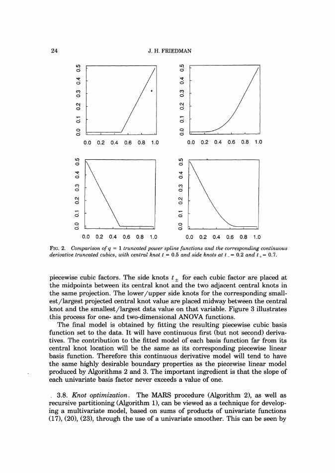
causes C(xls, t-, t, t+ ) to be continuous and have continuous first derivatives. There are second derivative discontinuities at x = ,.t Each truncated linear function (33) is characterized by a single knot location t, whereas each corresponding truncated cubic function (34), (35) is characterized by three knots; these are a central knot t and upper/lower side knots t,. Figure 2 compares the two functions.
Each factor (33) in every basis function in the approximation produced by Algorithms 2 and 3 (23) is replaced by a corresponding truncated cubic factor (34), (35;. The central knot t (34) is placed at the same location as the (single) knot for its associated truncated linear function (33). The side knots t,, t -< t < t+ , are located so as to reduce the number of second derivative discontinuities. This is accomplished through the ANOVA decomposition of the MARS model (24), (251, (261, (28).
Each basis function m in (23) has a knot set {tkm}fm. The ANOVA decom- position collects together all basis functions corresponding to exactly the same variable set {v(k, m)}fm. Thus, the knot sets associated with each ANOVA function (25), (26), (28) can be viewed as a set of points (multivariate knots) in the same Km-dimensional space. The projections of these points onto each of the respective K, axes, v(k, m), gives the knot locations of the factors that correspond to that variable. These are the central knot locations for the
J.H.FRIEDMAN
FIG.2. Comparison of q = 1 truncated power spline functions and the corresponding continuous derivative truncated cubics, with central knot t = 0.5 and side knots at t -= 0.2 and t+= 0.7.
piecewise cubic factors. The side knots t , for each cubic factor are placed at the midpoints between its central knot and the two adjacent central knots in the same projection. The lower/upper side knots for the corresponding small- est/largest projected central knot value are placed midway between the central knot and the smallest/largest data value on that variable. Figure 3 illustrates this process for one- and two-dimensional ANOVA functions.
The final model is obtained by fitting the resulting piecewise cubic basis function set to the data. I t will have continuous first (but not second) deriva- tives. The contribution to the fitted model of each basis function far from its central knot location will be the same as its corresponding piecewise linear basis function. Therefore this continuous derivative model will tend to have the same highly desirable boundary properties as the piecewise linear model produced by Algorithms 2 and 3. The important ingredient is that the slope of each univariate basis factor never exceeds a value of one.
, 3.8. Knot optimization. The MARS procedure (Algorithm 2), as well as recursive partitioning (Algorithm I),can be viewed as a technique for develop- ing a multivariate model, based on sums of products of univariate functions (171, (20), (23), through the use of a univariate smoother. This can be seen by

MULTIVARIATE ADAPTIVE REGRESSION SPLINES
'a 'c'b I -- ,, 'i
'a- ' a t 'b+ 'c+ 'b- a 'c-
FIG.3. Illustration of side knot placement for a one-dimensional ANOVA function comprised of three basis functions (upper frame) and a two-dimensional ANOVA function with two basis functions (lower frame).
casting the (MARS) model in the form
with
The function pmu(x,) has the form
which is just a (q = 1)piecewise linear spline representation of a univariate function. (In the case of recursive partitioning, it would be a q = 0 piecewise constant representation.) The second term in (36) isolates the contributions to the model of the variable set V(m) of the mth basis function and the set including the variable v with V(m). The first term (37) represents the contri- butions of the variables from the other basis functions. Minimization of the lack-of-fit criterion (30) in Algorithm 2 (line 7) performs a joint optimization of

26 J.H. FRIEDMAN
the current model with respect to the coefficients (c,, . . . ,c,) of the univariate function cp,, (38) and those of the other basis functions {ai}(37).
Expressing the current model in the form given by (36) and letting
this optimization can be written in the form
Here the dependence of the respective quantities on the multivariate argument x has been surpressed. If one fixes the values of the coefficients {ai}(37), then (40) has the general solution
which can be estimated by a weighted smooth of R\,,/Bm on xu, with weights given by B;. Letting this smooth take the form of a piecewise linear spline approximation (38) gives rise (in an indirect way) to the MARS ap- proach.
This framework provides the connection between MARS and the smoothing (and additive modeling) method (TURBO) suggested by Friedman and Silverman (1989). They presented a forward stepwise strategy for knot place- ment in a simple piecewise linear smoother. The inner For loop of Algorithm 2 can be viewed as an application of this strategy for choosing the best location for the next knot t , in cpm,(x,) (38), (41) in the more general context of MARS modeling. In fact, in the univariate case (n = I), the MARS algorithm simply represents a (palindromically invariant) version of TURBO. As noted earlier, restricting the upper limit of the outer For loop to always have the value one (Algorithm 2) gives rise (for n > 1) to the TURBO method of additive model- ing.
Both recursive partitioning (Algorithm 1, line 5) and MARS (Algorithm 2, line 5) make every distinct (nonzero weighted) marginal data value eligible for knot placement. As pointed out by Friedman and Silverman (1989), this has the effect of permitting the corresponding piecewise linear smoother (381, (41) to achieve a local minimum span of one observation. In noisy settings, this can lead to locally high variance of the function estimate. There is no way that a smoother, along with its lack-of-fit criterion, can distinguish between sharp structure in the true underlying function f (1) and a run of either positive or negative error values E (1). If one assumes (as one must) that the underlying function is smooth compared to the noise, then it is reasonable to impose a minimum span on the smoother that makes it resistant to runs in the noise of length likely to be encountered in the errors. In the context of piecewise linear smoothing, this translates into a minimal number L of (nonzero weighted) observations between each knot. Assuming a symmetric error distribution, Friedman and Silverman (1989) use a coin tossing argument to propose
MULTIVARIATE ADAPTIVE REGRESSION SPLINES
choosing L = L*/2.5 with L* being the solution to
(42) Pr( L*) = a.
Here Pr(L*) is the probability of observing a (positive or negative) run of length L* or longer in nNm tosses of a fair coin and a is a small number (say a = 0.05 or 0.01). The quantity Nm is the number of observations for which B , > 0 (Algorithm 2, line 5). The relevant number of tosses is nNm, since there are that many potential locations for each new knot (inner two For loops in Algorithm 2) for each basis function Bm (outer For loop).
For nNm 2 10 and a < 0.1, a good approximation to L* (42) is
so that a reasonable number of counts between knots is given by
The denominator in (43) arises from the fact that a piecewise linear smoother must place between two and three knots in the interval of the run to respond to it and not degrade the fit anywhere else. Using (43) gives the procedure resistance, with probability 1- a, to a run of positive or negative error values in the interior of the interval.
The arguments that lead to (43) do not apply to the ends of the interval; that is, L(a) refers to the number of counts between knots but not to the number of counts between the extreme knot locations and the corresponding ends of the interval defined by the data. As discussed in Section 3.7, it is essential that end effects be handled well for the procedure to be successful. An argument analogous to the one that leads to L(a) (43) for the interior, can be advanced for the ends. The probability of a run of length L* or longer of positive or negative error values at the beginning or end of the data interval is 2 - ~ * + 3. There are n such intervals, corresponding to the n predictor vari-
ables, so that the total probability of encountering an end run is
(44) Pr(L*) = 7 ~ 2 - ~ * + ~ .
Therefore requiring at least
(45) Le(a) = 3 - log,(a/n)
observations between the extreme knots and the corresponding ends of the interval provides resistance (with probability 1- a ) to runs at the ends of the data intervals.
The quantity a in (431, (45) can be regarded as another smoothing para- meter of the procedure. Both L(a) (43) and Le(a) (45) are, however, fairly insensitive to the value of a . The differences L(0.01) - L(0.05) and Le(O.01) - Le(0.05) are both approximately equal to 2.3 observations. In any

28 J.H. FRIEDMAN
case, both expressions can only be regarded as approximate since they only consider the signs and ignore the magnitudes of the errors in the run.
I t can be noted that (36), (37), (39) and (41) could be used to develop a generalized backfltting algorithm based on a (univariate) local averaging smoother, in direct analogy to the backfitting algorithm for additive modeling [Friedman and Stuetzle (1981), Breiman and Friedman (1985) and Buja, Hastie and Tibshirani (1989)l. Like MARS, this generalized backfitting algo- rithm could be used to fit models involving sums of products of univariate curve estimates. I t would, however, lack the flexibility of the MARS procedure (especially in high dimensions) owing mainly to the latter's close relation to the recursive partitioning approach (local variable subset selection-see Sec-tions 2.4.2 and 6). It would also tend to be computationally far more expensive.
3.9. Computational considerations. In Sections 3.2 and 3.3, the MARS procedure was motivated as a series of conceptually simple extensions to recursive partitioning regression. In terms of implementation, however, these extensions produce a dramatic change in the algorithm. The usual implemen- tations of recursive partitioning regression (AID [Morgan and Sonquist (1963)l and CART [Breiman, Friedman, Olshen and Stone (1984)l) take strong advan- tage of the special nature of step functions, along with the fact that the resulting basis functions have disjoint support, to dramatically reduce the computation associated with the middle and inner For loops of Algorithm 1 (lines 4 and 5). In the case of least-squares fitting, very simple updating formulae can be employed to reduce the computation for the associated linear (least-squares) fit (line 7) from O(NM2 + M3) to O(1). The total computation can therefore be made proportional to nNM,,, after sorting. Unfortunately, these same tricks cannot be applied to the implementation of the MARS procedure. In order to make it computationally feasible, different updating formulae must be derived for the MARS algorithm.
The minimization of the lack-of-fit criterion (30) in Algorithm 2 (line 7) is a linear least-squares fit of the response y on the current basis function set (line 6). There are a variety of techniques for numerically performing this fit. The most popular, owing to its superior numerical properties, is based on the QR decomposition [see Golub and Van Loan (1983)l of the basis data matrix B,
(46) Bmi= Bm(xi) .
As noted before, however, computational speed is of paramount importance since this fit must be repeated many times in the course of running the algorithm. A particular concern is keeping the computation linear in the number of observations N, since this is the largest parameter of the problem. This rules out the QR decomposition technique in favor of an approach based on using the Cholesky decomposition to solve the normal equations
(47) BTBa = BTy
for the vector of basis coefficients a (line 6). Here y is the (length N ) vector of response values. This approach is known to be less numerically stable than the

29 MULTIVARIATE ADAPTIVE REGRESSION SPLINES
QR decomposition technique. Also, the truncated power basis (21) is the least numerically stable representation of a spline approximation. Therefore, a great deal of care is required in the numerical aspects of an implementation of this approach. This is discussed later.
If the basis functions are centered to have zero mean, then the matrix product BTB is proportional to the covariance matrix of the current basis function set. The normal equations (47) can be written
with
and Biand 7 the corresporiding averages over the data. These equations (481, (491 must be resolved for every eligible knot location t , for every variable v, for all current basis functions m and for all iterations M of Algorithm 2 (lines 2, 3, 4 and 5). If carried out in a straightforward manner, this would require computation proportional to
with cu and p constants of proportionality and L given by (43). This computa- tional burden would be prohibitive except for very small problems or very large computers. Although it is not possible to achieve the dramatic reduction in computation for MARS as can be done for recursive partitioning regression, one can reduce the computation enough, so that moderate-sized problems can be conveniently run on small computers. Following Friedman and Silverman (19891, the idea is to make use of the special properties of the q = 1truncated power spline basis functions to develop rapid updating formulae for the quantities that enter into the normal equations (48), (491, as well as to take advantage of the rapid updating properties of the Cholesky decomposition [see Golub and Van Loan (1983)l.
The most important special property of the truncated power basis used here is that each (univariate) basis function is characterized by a single knot. Changing a knot location changes only one basis function, leaving the rest of the basis unchanged. Other bases for representing spline approximations, such as the minimal support B-splines, have superior numerical properties but lack this important computational aspect. Updating formulae for B-splines are therefore more complex giving rise to slower computation.
The current model (Algorithm 2, line 6) can be reexpressed as
30 J. H. FRIEDMAN
The inner For loop (line 5) minimizes the GCV criterion (30) jointly with respect to the knot location t and the coefficients a,, . . . ,a,+,. Using g' (51) in place of g (line 6) yields an equivalent solution with the same optimizing GCV criterion lof* (line 8) and knot location t* (line 8). (The solution coefficient values will be different.) The advantage of using g' (51) is that only one basis function is changing as the knot location t changes.
Friedman and Silverman (1989) developed updating formulae for least- squares fitting of q = 1 splines by visiting the eligible knot locations in decreasing order and taking advantage of that fact for t I u,
X l t - + - - + x - t t < x < u
( Ou - t . x 2 u .
The Friedman and Silverman (1989) updating formulae can be extended in a straightforward manner to the more general MARS setting, giving (t I u)
with s(t) = C x,k Brnk(xuk- t). In (521, B,, and B,, are elements of the basis function data matrix (46), the xu, are elemetlts of the original data matrix and y, are the data response values.
These updating formulae (52) can be used to obtain the last ( M + 1)st row (and column) of the basis covariance matrix V and last element of the vector c at all eligible knot locations t with computation proportional to ( M + 2)Nm. Here Nm is the number of observations for which Bm(x) > 0 (line 5). Note that all the other elements of V and c do not change as the knot location t changes. This permits the use of updating formulae for the Cholesky decompo- sition to reduce its computation from 0(M3) to O(M2) [in solving the normal equations (48)] at each eligible knot location. Therefore the computation required for the inner For loop (lines 5-9) is proportional to aMN, +
-pM2Nm/L. This gives an upper bound on total computation for Algorithm 2 as being proportional to
MULTIVARIATE ADAPTIVE REGRESSION SPLINES 31
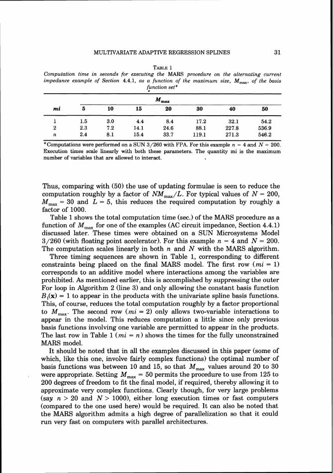
TABLE1 Computation time in seconds for executing the MARS procedure on the alternating current impedance example of Section 4.4.1, as a function of the maximum size, M,,, of the basis
Friction set*
Mm,
1 1.5 3.0 4.4 8.4 17.2 32.1 54.2 2 2.3 7.2 14.1 24.6 88.1 227.8 536.9 n 2.4 8.1 15.4 33.7 119.1 271.3 546.2
*Computations were performed on a SUN 3/260 with FPA. For this example n = 4 and N = 200. Execution times scale linearly with both these parameters. The quantity mi is the maximum number of variables that are allowed to interact.
Thus, comparing with (50) the use of updating formulae is seen to reduce the computation roughly by a factor of NM,,/L. For typical values of N = 200, M,, = 30 and L = 5, this reduces the required computation by roughly a factor of 1000.
Table 1shows the total computation time (sec.) of the MARS procedure as a function of M,, for one of the examples (AC circuit impedance, Section 4.4.1) discussed later. These times were obtained on a SUN Microsystems Model 3/260 (with floating point accelerator). For this example n = 4 and N = 200. The computation scales linearly in both n and N with the MARS algorithm.
Three timing sequences are shown in Table 1,corresponding to different constraints being placed on the final MARS model. The first row (mi = 1) corresponds to an additive model where interactions among the variables are prohibited. As mentioned earlier, this is accomplished by suppressing the outer For loop in Algorithm 2 (line 3) and only allowing the constant basis function B,(x) = 1to appear in the products with the univariate spline basis functions. This, of course, reduces the total computation roughly by a factor proportional to M,,. The second row (mi = 2) only allows two-variable interactions to appear in the model. This reduces computation a little since only previous basis functions involving one variable are permitted to appear in the products. The last row in Table 1(mi = n) shows the times for the fully unconstrained MARS model.
It should be noted that in all the examples discussed in this paper (some of which, like this one, involve fairly complex functions) the optimal number of basis functions was between 10 and 15, so that M,, values around 20 to 30 were appropriate. Setting M,, = 50 permits the procedure to use from 125 to 200 degrees of freedom to fit the final model, if required, thereby allowing it to approximate very complex functions. Clearly though, for very large problems (say n > 20 and N > 1000), either long execution times or fast computers (compared to the one used here) would be required. I t can also be noted that the MARS algorithm admits a high degree of parallelization so that it could run very fast on computers with parallel architectures.
32 J.H. FRIEDMAN
Updating formulae for higher order (q > 1) truncated power spline basis functions (21) can be developed in analogy to (52). They would, however, be far more complex than those for q = 1 leading to much slower execution of the algorithm. Also, their corresponding numerical properties would be very much worse.
At any point during the execution of Algorithm 2, the current basis function set need not be linearly independent. (The basis functions set comprising the final model is, however, always linearly independent.) Therefore, the covari- ance matrix V appearing in the normal equations (48) may be singular. This presents no fundamental problem since they can be solved by applying pivoting in the Cholesky decomposition [see Dongarra, Moler, Bunch and Stewart (1979)l. A better strategy from the point of view of MARS modeling is, however, to slightly modify the normal equations via
(54) (V + ED)^ = c ,
where D is a diagonal (M + 1) x ( M + 1) matrix comprised of the diagonal elements of V. The coefficients for the basis function set a are then taken to be the solution derived from (54). The average-squared residual
M + 1
(55) (y, - 412 - ai(c i + SD,,a,) k = l i = l I
is still used as the numerator of the GCV criterion (30). The value for S is taken to be a small number just large enough to maintain numerical stability.
The principal advantage of this ridge regression approach (54) is that it eliminates the need for pivoting in the Cholesky decomposition update, thereby increasing execution speed. Additional advantages are that it increases numeri- cal stability to help compensate for the bad numerical properties of the truncated power spline basis representation and it applies a small overall shrinkage to the solution coefficients to help compensate for the selection bias inherent in stepwise regression procedures [see Copas (1983)l.
The updating formulae (52) are not necessarily numerically stable. Widely different locations and scales for the predictor variables can cause instabilities that adversely effect the quality of the final model. The MARS procedure is (except for numerics) invariant to the locations and scales of the predictor variables. I t is therefore reasonable to perform a transformation that causes the resulting locations and scales to be most favorable from the point of view of numerical stability. Standardizing them to each have zero location and unit scale provides good numerical properties.
4. Simulation studies and examples. In the following sections we present the results of applying the MARS procedure to a series of simulated and real data sets. The goal is to try to gain some understanding of its properties and to learn in what situations one might expect it to provide better performance than existing methodology. In all the examples the smoothing parameter d (32) was taken to be d = 3. The software automatically reduces it to 2d/3 (= 2) for additive modeling. The minimum number of observations
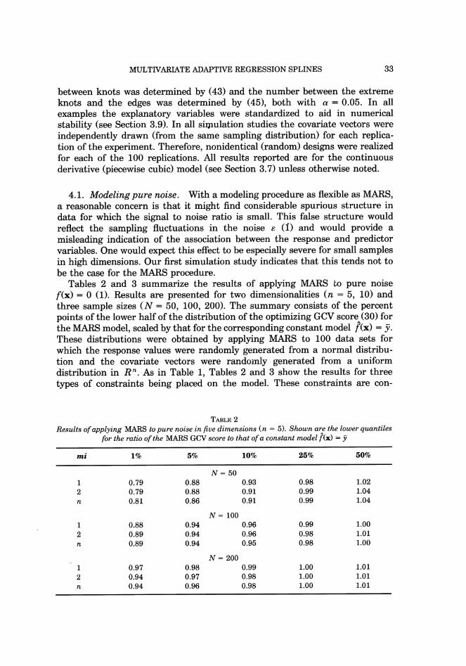
33 MULTIVARIATE ADAPTWE REGRESSION SPLINES
between knots was determined by (43) and the number between the extreme knots and the edges was determined by (45), both with a = 0.05. In all examples the explanatory variables were standardized to aid in numerical stability (see Section 3.9). In all simulation studies the covariate vectors were independently drawn (from the same sampling distribution) for each replica- tion of the experiment. Therefore, nonidentical (random) designs were realized for each of the 100 replications. All results reported are for the continuous derivative (piecewise cubic) model (see Section 3.7) unless otherwise noted.
4.1. Modeling pure noise. With a modeling procedure as flexible as MARS, a reasonable concern is that it might find considerable spurious structure in data for which the signal to noise ratio is small. This false structure would reflect the sampling fluctuations in the noise E (I) and would provide a misleading indication of the association between the response and predictor variables. One would expect this effect to be especially severe for small samples in high dimensions. Our first simulation study indicates that this tends not to be the case for the MARS procedure.
Tables 2 and 3 summarize the results of applying MARS to pure noise f(x) = 0 (1). Results are presented for two dimensionalities (n = 5, 10) and three sample sizes ( N = 50, 100, 200). The summary consists of the percent points of the lower half of the distribution of the optimizing GCV score (30) for the MARS model, scaled by that for the corresponding constant model f(x) = 7. These distributions were obtained by applying MARS to 100 data sets for which the response values were randomly generated from a normal distribu- tion and the covariate vectors were randomly generated from a uniform distribution in Rn. As in Table 1, Tables 2 and 3 show the results for three types of constraints being placed on the model. These constraints are con-
TABLE2 Results of applying MARS to pure noise in five dimensions ( n = 5 ) . Shown are the lower quantiles
for the ratio of the MARS GCV score to that of a constant model f (x) =
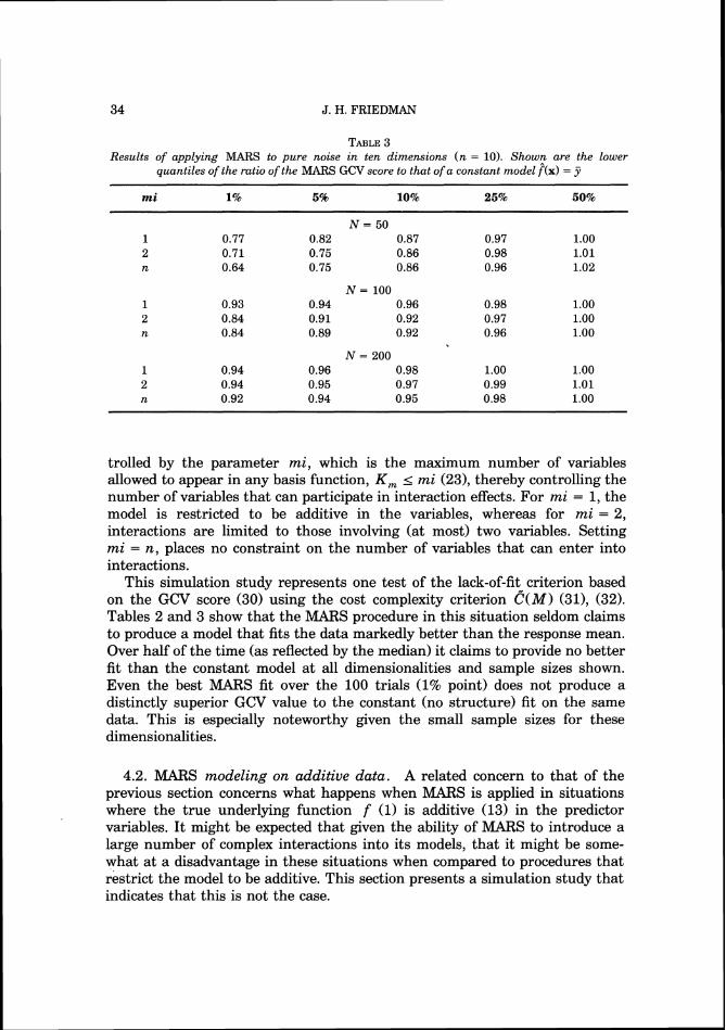
34 J.H. FRIEDMAN
TABLE3 Results of applying MARS to pure noise in ten dimensions ( n = 10). Show? are the lower
quantiles of the ratio of the MARS GCV score to that of a constant model f ( x ) = 4
trolled by the parameter m i , which is the maximum number of variables allowed to appear in any basis function, K , Imi (231, thereby controlling the number of variables that can participate in interaction effects. For mi = 1, the model is restricted to be additive in the variables, whereas for mi = 2, interactions are limited to those involving (at most) two variables. Setting mi = n , places no constraint on the number of variables that can enter into interactions.
This simulation study represents one test of the lack-of-fit criterion based on the GCV score (30) using the cost complexity criterion C ( M ) (31), (32). Tables 2 and 3 show that the MARS procedure in this situation seldom claims to produce a model that fits the data markedly better than the response mean. Over half of the time (as reflected by the median) it claims to provide no better fit than the constant model at all dimensionalities and sample sizes shown. Even the best MARS fit over the 100 trials (1% point) does not produce a distinctly superior GCV value to the constant (no structure) fit on the same data. This is especially noteworthy given the small sample sizes for these dimensionalities.
4.2. MARS modeling on additive data. A related concern to that of the previous section concerns what happens when MARS is applied in situations where the true underlying function f (1) is additive (13) in the predictor variables. I t might be expected that given the ability of MARS to introduce a large number of complex interactions into its models, that it might be some- what at a disadvantage in these situations when compared to procedures that restrict the model to be additive. This section presents a simulation study that indicates that this is not the case.

35 MULTIVARIATE ADAPTIVE REGRESSION SPLINES
We use for this study an example presented in Friedman and Silverman (1989)
This function has a nonlinear additive dependence on the first two variables, a linear dependence on the next three and is independent of the last five (pure noise) variables. A simulation study was performed consisting of 100 replica- tions of the following experiment. First N(= 50,100,200) 10-dimensional (n = 10) covariate vectors were generated in the unit hypercube. Then corre- sponding response values were assigned according to ,
with the cirandomly generated from a standard normal and f(x) given by (56). Here the signal-to-noise ratio is 3.28 so that the true underlying function (56) accounts for 91% of the variance of the response (57).
A reasonable strategy to be used with MARS modeling is to fit both an additive model (mi = 1) and one that permits interactions (mi = 2 or mi = n). The respective GCV scores of both models can then be compared and the one corresponding to the lowest score chosen. With this strategy a model involving interactions is only used if it claims (through its GCV score) to do better than an additive model on the same data.
For each of the 100 replications (at each sample size N), the MARS procedure was applied with mi = 1, 2 and n. The first value (mi = 1) corre- sponds to additive modeling, the second (mi = 2) permits interactions in at most two variables, whereas the last (mi = n = 10) fits an unconstrained MARS model. For the last two mi values, the corresponding interaction fit was only used if it produced a smaller GCV score than the additive model on the same data.
Table 4 compares the average accuracy of using this strategy to that of additive modeling on the purely additive data (56), (57). The principal measure of accuracy is the (scaled) integral-squared error ISE (2), (29),
ISE = / [ f ( x ) - f (x ) ,f ( ~ ) ] ~ d " x , / v a r D X E D
where here n = 10 and D is the 10-dimensional unit hypercube. For each replication of the simulation study, the ISE (58) was estimated by Monte Carlo integration using 5000 points randomly generated from a uniform distribution over D.
A closely related quantity of interest is the (scaled) predictive-squared error
(59) PSE = E [ y - f (x)]'/vary

36 J. H. FRIEDMAN
TABLE4 Comparison of the accuracy of MARS modeling, with interactions permitted ( m i = 2, lo), to that
ofpurely additive modeling ( m i = 1) on aaditive data (Section 4.2)
- * -ISE PSE GCV / PSE
which is related to the ISE (58) by
(60) PSE = (ISE . Var f (x) + Var &) /vary , XED
with F being the error component (1). If the response values y,, . . . ,y, y e standardized to have unit variance, then the GCV criterion (30), (31), (32) is intended as an estimate of the PSE (591, (60) and the ratio GCV/PSE provides an estimate of how well the optimized GCV criterion for the model is estimat- ing the true PSE.
Shown in Table 4 are the average ISE (581, PSE (59) and GCV/PSE, along with the corresponding standard deviations (in parentheses) over the 100 replications at each sample size N(= 50,100,200). (Note that the standard deviations of the averages shown in the table are one-tenth the corresponding standard deviations shown.) Comparing the first row (mi = 1) to the next two (mi = 2, n ) shows that there is little sacrifice in accuracy using interaction models in the context of the earlier strategy, even though the true underlying function (56) involves no interactions. Table 4 also shows that the optimized GCV score produced by the MARS fit slightly overestimates (on average) the actual predictive-squared error for this problem at all sample sizes studied. This effect is most pronounced for the smallest sample size ( N = 50). (Note that the variability of this ratio as reflected by its standard deviation over the 100 replications is fairly high.)
The previous strategy chooses the additive model over that involving inter- actions only if the former produces a GCV score no worse than the latter. The first column of Table 5 shows the number of times the additive model was chosen in the 100 replications of this simulation experiment. As can be seen, the additive model was being chosen most of the time. This is why the loss in
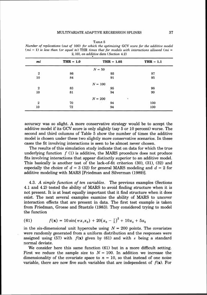
MULTIVARIATE ADAPTIVE REGRESSION SPLINES 37
TABLE5 Number of replications (out of 100) for which the optimizing GCV score for the additive model ( m i = 1) is less than (or equal to) THR times that for models with interactions allowed ( m i =
2, lo), on additive data (Section 4.2) 8
mi THR = 1.0 THR = 1.05 THR = 1.1
accuracy was so slight. A more conservative strategy would be to accept the additive model if its GCV score is only slightly (say 5 or 10 percent) worse. The second and third columns of Table 5 show the number of times the additive model is chosen under these two slightly more conservative scenarios. In these cases the fit involving interactions is seen to be almost never chosen.
The results of this simulation study indicate that on data for which the true underlying function f (1) is additive, the MARS procedure does not produce fits involving interactions that appear distinctly superior to an additive model. This basically is another test of the lack-of-fit criterion (30), (311, (32) and especially the choice of d = 3 (32) for general MARS modeling and d = 2 for additive modeling with MARS [Friedman and Silverman (1989)l.
4.3. A simple function of ten variables. The previous examples (Sections 4.1 and 4.2) tested the ability of MARS to avoid finding structure when it is not present. It is at least equally important that it find structure when it does exist. The next several examples examine the ability of MARS to uncover interaction effects that are present in data. The first test example is taken from Friedman, Grosse and Stuetzle (1983). They considered trying to model the function
in the six-dimensional unit hypercube using N = 200 points. The covariates were randomly generated from a uniform distribution and the responses were assigned using (57) with f(x) given by (61) and with E being a standard normal deviate.
We consider here this same function (61) but in a more difficult setting. First we reduce the sample size to N = 100. In addition we increase the dimensionality of the covariate space to n = 10, so that instead of one noise variable, there are now five such variables that are independent of f(x). For

38 J. H. FRIEDMAN
TABLE6 Summary of the MARS model for the data of Section 4.3*
Fun. a \GCV #Basis #Palms Variableh)
1 0.56 0.67 1 2.8 4 2 0.29 0.087 1 2.8 2 3 0.50 0.26 1 2.8 1 4 0.28 0.21 1 2.8 5 5 0.30 0.22 2 5.7 3 6 0.46 0.37 4 11.3 1 2 7 0.064 0.059 1 2.8 2 6
*GCV (piecewise-linear) = 0.059; GCV (piecewise-cubic) = 0.055; total number of basis functions = 11; total effective number of parameters = 32.3. ANOVA decomposition.
this study however, the MARS procedure has no prior knowledge of the nature of the dependence of f(x)on any of the variables. The signal-to-noise ratio for this example is high (4.8/1); the true underlying function accounts for 96% of the variance of the response. On the other hand, the dimension of the covariate space is high ( n = 101, the sample is small ( N = 100) and the function (61) is fairly highly structured.
Table 6 summarizes the MARS model derived from a data set generated from the previous prescription. The data response values were standardized so that the resulting GCV scores are an estimate of the PSE (59). The table caption gives the optimizing GCV scores for the corresponding piecewise linear (23) and piecewise cubic (Section 3.7) fits, the total number of (nonconstant) basis functions M in the final model, and C(M) (31), (32), the estimated number of linear degrees of freedom used in the fit. The ANOVA decomposi- tion is summarized by one row for each ANOVA function. The columns represent summary quantities for each one. The first column lists the function number. The second gives the standard deviation of the function. This gives one indication of its (relative) importance to the overall model and can be interpreted in a manner similar to a standardized regression coefficient in a linear model. The third column provides another indication of the importance of the corresponding ANOVA function, by listing the GCV score for a model with all of the basis functions corresponding to that particular ANOVA function removed. This can be used to judge whether this ANOVA function is making an important contribution to the model, or whether it just slightly helps to improve the global GCV score. The fourth column gives the number of basis functions comprising the ANOVA function while the fifth column pro- vides an estimate of the additional number of linear degrees of freedom used by including it. The last column gives the particular predictor variables associated with the ANOVA function.
The MARS fit is seen in Table 6 to have produced seven ANOVA functions, the first five involving only one variable (K,= 1)and two comprised of two variables (K,= 2). Judging from the second and (especially) the third columns, the last ANOVA function (involving an interaction between variables 2 and 6)
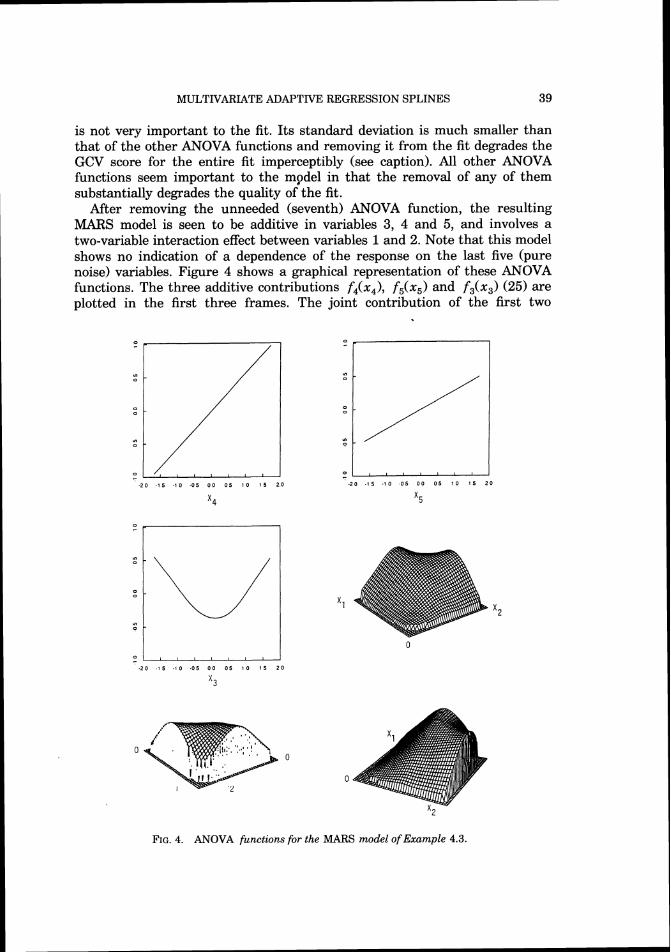
39 MULTIVARIATE ADAPTIVE REGRESSION SPLINES
is not very important to the fit. Its standard deviation is much smaller than that of the other ANOVA functions and removing it from the fit degrades the GCV score for the entire fit imperceptibly (see caption). All other ANOVA functions seem important to the mgdel in that the removal of any of them substantially degrades the quality of the fit.
After removing the unneeded (seventh) ANOVA function, the resulting MARS model is seen to be additive in variables 3, 4 and 5, and involves a two-variable interaction effect between variables 1and 2. Note that this model shows no indication of a dependence of the response on the last five (pure noise) variables. Figure 4 shows a graphical representation of these ANOVA functions. The three additive contributions f4(x4), f5(x5) and f3(x3) (25) are plotted in the first three frames. The joint contribution of the first two
FIG.4. ANOVA functions for the MARS model of Example 4.3.

- -
40 J. H. FRIEDMAN
variables f,T,(x,, x,) (27) is presented in three different views of a perspective mesh plot of this function (last three frames). Low values of the corresponding variables are indicated by the position of the 0, whereas higher values are in the direction of the axis label. Note that the plotting routine does not show the bivariate function outside the convex hull of the projected data points. As discussed in Section 3.7, the MARS procedure basically extrapolates linearly beyond the boundaries of the data. It is important to note that this surface does not represent a smooth of y on x, and x,, but rather it shows the contribution of x, and x, to a smooth of y on the ten variables x,, . . . ,x,,.
Comparing the results of the MARS fit to these data (Table 6 and Figure 4) with the true underlying function f(x) (61), shows that the resulting model provides a fairly accurate and interpretable description. This is especially noteworthy given the high dimensionality ( n = 10) and the small sample size ( N = 100).
Table 6 (and Figure 4) show results for one realization of a data set .vith N = 100. In order to assess the general ability of MARS to model data of this kind, it must be applied to a large number of realizations of this situation. Table 7 summarizes the results of running MARS on 100 replications of this example at three sample sizes ( N = 50, 100 and 200), in the same format as Table 4. (Here the strategy of choosing the additive fit if it produced a better GCV score was not used for the mi = 2,10 models.) For the very smallest sample size ( N = 501, the additive model (mi = 1) is seen to actually produce more accurate fits than those involving interactions (mi = 2,101, even though there are strong interaction effects (involving x, and x,) in the generated data. This is due to the bias-variance tradeoff. Even though the additive model is highly biased, its lower variance leads to lower estimation errors. When the sample size is increased, however, this is no longer the case and the models
TABLE7 Results of applying MARS to 100 data sets, at three sample sizes N , for the situation described in
Section 4.3
ISE PSE GCV / PSE

MULTIVARIATE ADAPTIVE REGRESSION SPLINES
FIG.5. Schematic diagram of the alternating current series circuit for Example 4.4.
involving interactions produce vastly superior accuracy. As in the additive case (Table 41, the optimized GCV criterion is seen to overestimate the actual PSE on average (again with fairly high sample-to-sample variability). I t is interest- ing to note that even though the true underlying function (61) exhibits interactions involving only two variables, the totally unconstrained MARS fit (mi = 10) produces models nearly as accurate as when the fit is constrained to have at most two-variable interactions (mi = 2).
4.4. Alternating current series circuit. Figure 5 shows a schematic dia- gram of a simple alternating current series circuit involving a resistor R, inductor L and capacitor C. Also in the circuit is a generator that places a voltage
( 6 2 4 Vab= V, sin wt
across the terminals a and b. Here w is the angular frequency which is related to the cyclic frequency f by
(62b) w = 2%-f. The electric current Iab that flows through the circuit is also sinusoidal with the same frequency,
( 6 2 ~ ) lab= (K/Z)sin(wt - 4 ) .
Its amplitude is governed by the impedance Z of the circuit and there is a phase shift 4 , both depending on the components in the circuit:
Z = Z ( R , o, L , C) ,
4 = 4 ( R , w , L , C ) . From elementary physics one knows that
4 ( R , w, L , C ) = tan-' I The purpose of this exercise is to see to what extent the MARS procedure can
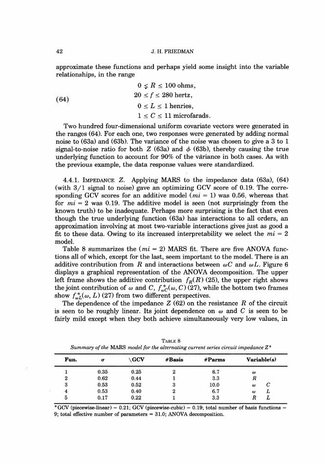
42 J. H. FRIEDMAN
approximate these functions and perhaps yield some insight into the variable relationships, in the range
0 jR I 100 ohms, 20 I f I 280 hertz,
0 5 L 5 1henries,
15 C 5 11microfarads.
Two hundred four-dimensional uniform covariate vectors were generated in the ranges (64). For each one, two responses were generated by adding normal noise to (63a) and (63b). The variance of the noise was chosen to give a 3 to 1 signal-to-noise ratio for both Z (63a) and 4 (63b), thereby causing the true underlying function to account for 90% of the vzh-iance in both cases. As with the previous example, the data response values were standardized.
4.4.1. IMPEDANCE Applying MARS to the impedance data (63a), (64) Z. (with 3/1 signal to noise) gave an optimizing GCV score of 0.19. The corre- sponding GCV scores for an additive model (mi = 1) was 0.56, whereas that for mi = 2 was 0.19. The additive model is seen (not surprisingly from the known truth) to be inadequate. Perhaps more surprising is the fact that even though the true underlying function (63a) has interactions to all orders, an approximation involving at most two-variable interactions gives just as good a fit to these data. Owing to its increased interpretability we select the mi = 2 model.
Table 8 summarizes the (mi = 2) MARS fit. There are five ANOVA func- tions all of which, except for the last, seem important to the model. There is an additive contribution from R and interactions between wC and w L. Figure 6 displays a graphical representation of the ANOVA decomposition. The upper left frame shows the additive contribution fR(R) (251, the upper right shows the joint contribution of o and C, f,*c(w, C) (271, while the bottom two frames show f,*,(o, L) (27) from two different perspectives.
The dependence of the impedance Z (62) on the resistance R of the circuit is seen to be roughly linear. Its joint dependence on o and C is seen to be fairly mild except when they both achieve simultaneously very low values, in
TABLE8 Summary of the MARS model for the alternating current series circuit impedance Z*
Fun. u \GCV #Basis #Parms Variablek)
*GCV (piecewise-linear) = 0.21; GCV (piecewise-cubic) = 0.19; total number of basis functions =
9; total effective number of parameters = 31.0; ANOVA decomposition.
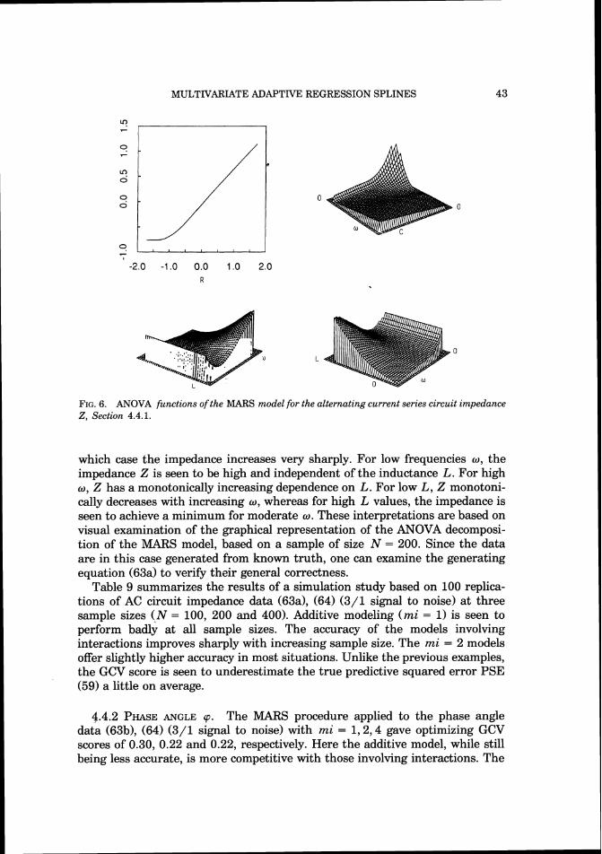
MULTIVARIATE ADAPTIVE REGRESSION SPLINES
FIG.6. ANOVA functions of the MARS model for the alternating current series circuit impedance 2,Section 4.4.1.
which case the impedance increases very sharply. For low frequencies w, the impedance Z is seen to be high and independent of the inductance L. For high w, Z has a monotonically increasing dependence on L. For low L, Z monotoni-cally decreases with increasing w, whereas for high L values, the impedance is seen to achieve a minimum for moderate w. These interpretations are based on visual examination of the graphical representation of the ANOVA decomposi- tion of the MARS model, based on a sample of size N = 200. Since the data are in this case generated from known truth, one can examine the generating equation (63a) to verify their general correctness.
Table 9 summarizes the results of a simulation study based on 100 replica- tions of AC circuit impedance data (63a), (64) (3/1 signal to noise) at three sample sizes (-N = 100, 200 and 400). Additive modeling (mi = 1) is seen to perform badly at all sample sizes. The accuracy of the models involving interactions improves sharply with increasing sample size. The mi = 2 models offer slightly higher accuracy in most situations. Unlike the previous examples, the GCV score is seen to underestimate the true predictive squared error PSE (59) a little on average.
4.4.2 PHASEANGLE 9. The MARS procedure applied to the phase angle data (63b), (64) (3/1 signal to noise) with mi = 1 ,2 ,4 gave optimizing GCV scores of 0.30, 0.22 and 0.22, respectively. Here the additive model, while still being less accurate, is more competitive with those involving interactions. The

- -
44 J. H. FRIEDMAN
TABLE9 Results of applying MARS to 100 data sets, at each of three sample sizes N , for the alternating
current impedance Z example
ISE PSE GCV / PSE
model limited to two-variable interactions (mi = 2) is again seen to fit the data as well as the general (mi = 4) MARS model. Table 10 summarizes the mi = 2 model. It involves nine ANOVA functions, two of which are clearly unimpor- tant (6 and 7) and three more that are of marginal importance (5, 8 and 9). Figure 7 shows perspective mesh plots of all six bivariate functions f * (27) associated with the four variables. The dependence of the phase angle cp on all of the variables is seen to be more gentle and more nearly additive than the impedance Z (Figure 6).
Table 11gives the results of applying MARS to 100 replications of the phase angle data at N = 100, 200 and 400. At the smallest sample size, additive fitting is seen to be almost as accurate as with interactions. This is, however,
TABLE10 Summary of the MARS model for the alternating current series circuit phase angle cp*
Fun. u \GCV #Basis #Parms Variablek)
1 0.45 0.32 2 5.6 w 2 0.86 0.34 2 5.6 C 3 0.62 0.38 2 5.6 L 4 0.42 0.26 3 8.4 R C 5 0.23 0.21 1 2.8 W L 6 0.12 0.19 1 2.8 L C 7 0.14 0.19 1 2.8 W C
;. 8 0.28 0.22 1 2.8 R L 9 0.24 0.23 1 2.8 R w
*GCV (piecewise-linear) = 0.19; GCV (piecewise-cubic) = 0.22; total number of basis functions =
14; total effective number of parameters = 40.2; ANOVA decomposition.

- -
MULTIVARIATE ADAPTrVE REGRESSION SPLINES
FIG.7 . ANOVA functions of the MARS model for the alternating current series circuit phase angle cp, Section 4.4.2.
TABLE11 Results of applying MARS to 100 data sets, at each of three sample sizes N , for the alternating
current phase angle cp example
ISE PSE GCV / PSE
J. H. FRIEDMAN
TABLE12 Measured variables for the Portuguese olive oil data
C16:O palmitic acid C16:l palmitoleic acid C17:O heptadecanoic acid C17:l heptadecenoic acid C18:O stearic acid C18:l oleic acid C18:2 linoleic acid C18:3 linolenic acid C20:O eicosanoic acid C24:O lignoceric acid Beta-sitosterol Carnpesterol Stigmasterol
no longer true at the larger sample sizes. The optimizing GCV score is seen to slightly underestimate the true PSE (on average) for most of the situations, but as with the previous examples, the variance of the ratio (GCV/PSE) dominates this small bias.
4.5. Portuguese olive oil. For this example, MARS is applied to data from analytical chemistry. The observations consist of 417 samples of olive oil from Portugal [Forina, Armanino, Lanteri, Calcagno and Tiscornia (1983)l. On each sample, measurements were made on the concentrations of 10 acids and three sterols (see Table 12). Also recorded was the location where the sample originated. The purpose was to see if there is a relation between the chemical composition and geographical origin. Of particular interest was the extent to which olive oil from northeastern Portugal (Douro Valley-90 samples) dif- fered from that of the rest of Portugal (327 samples). One way to address this question is to examine the results of trying to model the probability that a sample originates from the Douro Valley given its measured chemical composi- tion (Table 12). The response variable y in this case takes on only two values: 1= Duoro Valley, 0 = rest of Portugal. Since Pr(y = 11x1 = E(ylx), one can estimate this probability through regression techniques.
Linear logistic regression [Cox (1970)l is often used when the response variable assumes only two values. The model takes the form
n
log[p/(l - P)I = Po + C @,xi, i = l
where p is the probability that y assumes its larger value. The coefficients {Pi): are estimated by (numerically) maximizing the likelihood of the data. as tie and Tibshirani (1986) extended this approach to additive logistic regres-
sion n

47 MULTIVARIATE ADAPTIVE REGRESSION SPLINES
The smooth covariate functions are estimated through their local scoring algorithm. The model can be further generalized to involve potential interac- tion effects by a
with f(x) taking the form of the MARS approximation. This can be imple- mented in the MARS algorithm by simply replacing the internal linear least- squares routine (LOF-Algorithm 2, line 7 and Algorithm 3, lines 2 and 5) by one that does linear logistic regression (given the current set of multivariate spline basis functions). Unless rapid updating formulae can be derived, this is likely to be quite computationally intensive. A compromise strategy, however, is likely to provide a good approximation; the multivariate spline basis func- tions are selected using the MARS squared-error-based loss criterion, and the coefficients {a,}? for the final model are fit csing a linear logistic regression on this basis set. In this mode, one takes advantage of the local variable subset selection aspect of MARS as well as its ability to produce continuous models. The detailed knot placement on the selected variables will, however, be opti- mally placed for the untransformed response rather than for the logistic fit.
Table 13 gives the results of six different analyses (rows) on the Portuguese olive oil data set. The first column describes the method. The first two rows are for MARS runs on the untransformed 0/1 response using its least-squares criterion. The next two rows give results when a post (linear) logistic regres- sion is applied to the final basis function set as described earlier. The parame- ter mi is (as before) the maximum number of variables permitted in any basis function (mi = 1gives an additive model; mi = 2 allows two variable interac- tions). The last two rows are (respectively) ordinary stepwise linear logistic regression and recursive partitioning [CART: Breiman, Friedman, Olshen and Stone (1984)l. The second column gives the number of variables that entered each final model; the third column gives the GCV estimate of the PSE (59); the fourth column gives another estimate of this quantity (CV) based on 10-fold
TABLE13 Portuguese olive oil
Method #Vars GCV CV Error (CV)
MARS ( m i = 1) 3 0.23 0.21 0.050 (least-squares)
MARS ( m i = 2 ) 3 0.19 0.20 0.038 (least-squares)
MARS ( m i = 1) 3 0.16 0.19 0.036 (logistic)
MARS ( m i = 2) 3 0.13 0.16 0.026 (logistic)
linear logistic 4 0.25 0.26 0.070 (stepwise) CART 2 - 0.22 0.058

cross-validation; and the last column gives the cross-validated error rate of a prediction rule that assigns 9 = 1 if the estimated conditional probability ~ ( y l x )is greater than 0.5 and assigns 9 = 0 otherwise. In the case of logistic regression, the GCV and CV sdres were computed using as a (squared-error) loss function
with ?(XI the corresponding MARS estimate of the log-odds (65). Table 13 indicates that the (post) logistic transformation improves the fit
substantially. The GCV and CV estimates are seen to be fairly close, especially for the (untransformed) least-squares fits. The introduction of interaction effects (mi = 2) seems to improve the quality of the fit, especially for the logistic models. (Increasing the value for mi beyond 2 did not result in further improvement.) CART and stepwise linear logistic regression do not perform as well as the logistic MARS model involving two variable interactions on these data, although (like MARS) they do indicate a strong association between geographical origin (Douro Valley versus rest of Portugal) and the chemical composition (Table 12) of the olive oil samples. This (strong) association can be expressed with a small fraction of the 13 original predictor variables. [When using GCV or CV scores for comparisons it should be remembered that they not only estimate the accuracy of the approximation (2), (3) but also include the irreducible (binomial) error. Therefore their ratios understate the actual accuracy ratios of the methods being compared.]
Table 14 provides a summary of the logistic (mi = 2) MARS model. There are four ANOVA functions involving three (of the 13) predictor variables. All four ANOVA functions appear important to the fit, including the last two that involve interactions. Figure 8 shows the joint contribution (to the log-odds) of the second and twelft,h variables f,T,,(x,, x,,) (27) in the upper left frame and fCl2(x6, x12) in the upper right frame. The two lower frames show the same two plots, respectively, from a different perspective. The MARS model for the log-odds is (in this case) the sum of these two bivariate functions.
4.6. Low dimensional modeling. The main advantage of MARS modeling over existing methodology is clearly realized in high dimensional settings. I t is,
TAEILE14 Summary of the ( m i = 2) logistic MARS model for the Portuguese olive oil example*
Fun \GCV #Basis #Parms Variablek)
*Piecewise-linear: GCV = 0.10, CV = 0.15; piecewise-cubic: GCV = 0.13, CV = 0.15; total num- ber of basis functions = 9; total effective number of parameters = 29.5; ANOVA decomposition.

MULTIVARIATE ADAPTIVE REGRESSION SPLINES
FIG.8. ANOVA functions for the log-odds MARS model on the Portuguese olive oil data, Section 4.5.
however (unlike recursive partitioning), competitive in low dimensions (n I 2) as well. Friedman and Silverman (1989) studied its properties for the nonpara- metric smoothing problem (n = 1) and showed that it can produce superior performance especially in situations involving small samples and low signal to noise. [They also showed that for additive modeling (13) (n > 1, mi = 11, it is quite competitive with procedures based on the backfitting algorithm using local averaging smoothers.] In the univariate case (n = I), the MARS method can be viewed as a modification of an approach first suggested by Smith (1982). In a massive simulation study, Breiman and Peters (1988) ghowed that this was one of the best all around smoothers of those they tested.
In this section, we illustrate the use of MARS for two-dimensional nonpara- metric smoothing (n = 2). The first example is taken from Andrews and Herzberg (1985). The data comes from an experiment on the recoiling of guns [Brouncker (1734)l. A total of 109 shots were fired at different distances D between the muzzle and the target and with varying grains of powder in the charge C. The upper left frame of Figure 9 shows the experimental design. Note that there are 40 distinct points in the design so that some points represent more than one firing. The response variable is the (standardized) distance by which the resulting shot missed the target.
The MARS procedure applied to these data resulted in a model with three basis functions and an optimized GCV score of 0.39. The upper right and lower left frames of Figure 9 show two views of the MARS surface smooth. The average shooting error is seen to increase linearly with shooting distance for all powder charges. As might be expected, at the shortest distance, the error is very small and independent of the size of the powder charge. As the distance increases, the dependence of the shooting error on charge becomes nonmono-

J. H. FRIEDMAN
FIG.9. Experimental design (upper left) and MARS surface smooth for the gun recoil data, first example, Section 4.6.
tonic with the degree of nonmonotonicity increasing with shooting distance. The optimal (lowest shooting error) charge is seen to increase somewhat as the distance increases. This error is seen to be asymmetric about the minimum with the degree of asymmetry increasing with distance. For moderate to large distances it appears to be much more costly (in terms of average accuracy) to shoot with too small a powder charge than with one that is too large.
Our second example is an artificial one used by Gu, Bates, Chen and Wahba (1990) to illustrate interaction spline smoothing (see Section 2.3). They gener- ated 300 points (more or less) randomly from a uniform distribution in the unit square and set the response to
The errors E~ were drawn from a standard normal distribution. Here the signal to noise is 3.15/1 so that the true underlying function accounts for about 91% of the variance of the response. Figure 10 shows a mesh plot of the true underlying function y - E (66) over the unit square.
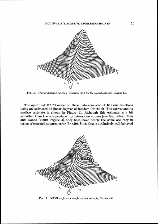
MULTIVARIATE ADAPTIVE REGRESSION SPLINES
True underlying function [equation (6611 for the second example, Section
The optimized MARS model on these data consisted of 18 basis functions using an estimated 45 linear degrees of freedom for the fit. The corresponding surface estimate is shown in Figure 11. Although this estimate is a bit smoother than the one produced by interaction splines [see Gu, Bates, Chen and Wahba (1990), Figure 41, they both have nearly the same accuracy in terms of expected squared error (3), (29). Since this is a relatively well-behaved
V
FIG.11. MARS surface smooth for second example, Section 4.6.

52 J. H. FRIEDMAN
function and the sample size is quite large ( N = 300), it is likely that methods based on kernel smoothing [Cleveland and Devlin (1988)l and (nonadaptive) tensor product splines [de Boor (197811 would also do well in this case.
Although MARS is competitive with other methodologies in low dimensions, what sets it apart is its ability to handle problems involving many variables. Suppose the variables (x,, x,) in (66) were two out of ten variables, all of which (jointly) effect the response y in an unknown way, and the goal is to estimate the dependence of the response on x,, x,, accounting for the effect of the other eight (nuisance) variables x,, . . . ,x,,. To get an idea of how well MARS might do in such a problem, N = 300 points were generated in the n = 10 dimen- sional unit hypercube. The dependence of this response j j was taken to be
(67) . f i = ~ i + f ( x , ) , . with y, given by (66) and f(x) given by (61) (shifted by two arguments). Thus, the dependence of j j on the first two variables is the same as in the previous two-dimensional example, whereas its dependence on the last eight is the same as the first eight variables of the problem studied in Section 4.3. The sample size ( N = 300) and the pure noise level are the same as in the two-dimensional problem. The apparent noise in the x,x,-plane is now however many times greater owing to the variability induced in the response by the many nuisance variables. I t is hoped that one can account for the variance associated with the nuisance variables by fitting a (nonparametric) model jointly with respect to them and the variables of interest, thereby obtaining a better estimate of the dependence of the response on x,, x,.
Applying MARS to this 10-dimensional data resulted in a model with 27 basis functions using an estimated 68.5 linear degrees of freedom. Eleven of the basis functions were associated with the dependence on variables x, and x,, accounting for 27.5 linear degrees of freedom. Figure 12 shows the result- ing surface estimate. Although it is not quite as accurate as the smooth (Figure 11) produced in the absence of the eight nuisance variables, it still gives a good indication of the nature of the joint dependence of the response on x, and x,. The estimate (Figure 12) is smoother than that of Figure 11owing to the fact that it is based on 11 rather than 18 basis functions. Figure 13 shows plots of all the ANOVA functions produced by the MARS fit to the 10-dimensional data. The estimates corresponding to the (nuisance) variables associated with f(x) (61), (67) are actually better than those obtained in the example of Section 4.3. This is the result of having 300 observations h?re, whereas only 100 were used in Section 4.3.
4.7. Slicing a MARS model. In the examples presented so far, the domi- nant interactions involved at most two variables. The resulting MARS models could then be visualized through plots of the contributing ANOVA functions (251, (27). When substantial interaction effects involving more than two vari- ables are present, the model becomes more difficult to interpret. This section describes an interpretational tool called slicing that can aid in the visualization of such models.

MULTIVARIATE ADAPTIVE REGRESSION SPLINES
FIG. 12. MARS surface smooth for the second example, Section 4.6, i n the presence of eight highly structured nuisance variables.
The MARS model (23), (34) is a sum of products of univariate functions
Here bkmis either a q = 1spline basis function (33) or its cubic analog (34). If the number of factors K m in any product is greater than two, then f(x) is more difficult to interpret since the ANOVA decomposition (24) contains functions of more than two variables which are difficult to plot or visualize. It is possible, however, to get a rough idea of the behavior of f(x) by reducing the dimensionality of the predictor variable space by repeatedly conditioning on subsets of the variables.
Let Z represent a (selected) subset of the predictor variables ( 2 , . . . x,), with dimension d ( < n ) and z the complement subset of dimension n - d . Define a d-dimensional slice of the predictor variable space by simultaneously assigning specific values to the selected variables
(69) slice: {Z, = z,, . . . ,Z, = z,) = Z = z.
The MARS model along the slice will be a function of the variables 2 complement to those defining the slice
The particular form of the MARS model (68) makes the sliced model (70)

J.H.FRIEDMAN
l
FIG. 13. ANOVA functions for the ten-variable version of the second example in Section 4.6.
especially straightforward to compute by decomposing its products into those factors involving variables defining the slice, and those involving the comple- ment variables,
For a given slice (Z = z), the first product in (71) evaluates to a constant (inultiplying the coefficient a,) and the second product gives the dependence on the complement variables. The MARS model along the slice can therefore
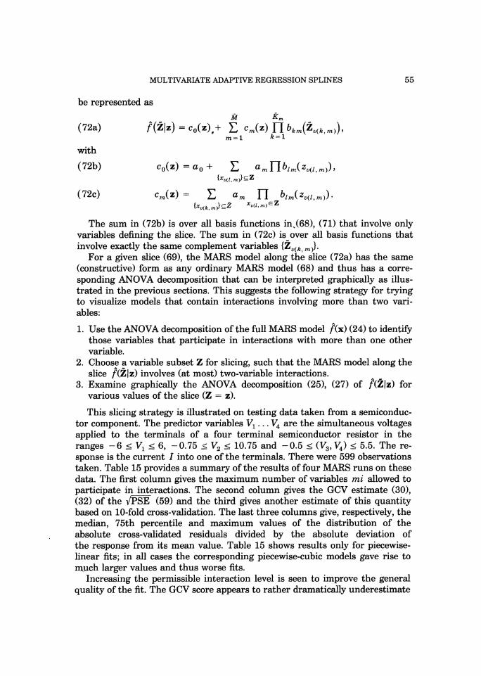
MULTIVARIATE ADAPTNE REGRESSION SPLINES
be represented as
with
The sum in (72b) is over all basis functions in,(68), (71) that involve only variables defining the slice. The sum in (72c) is over all basis functions that involve exactly the same complement variables {z,,,, ,,).
For a given slice (69), the MARS model along the slice (72a) has the same (constructive) form as any ordinary MARS model (68) and thus has a corre- sponding ANOVA decomposition that can be interpreted graphically as illus- trated in the previous sections. This suggests the following strategy for trying to visualize models that contain interactions involving more than two vari- ables:
1. Use the ANOVA decomposition of the full MARS model f(x) (24) to identify those variables that participate in interactions with more than one other variable.
2. Choose a variable subset Z for slicing, such that the MARS model along the slice f ( ~ l z ) involves (at most) two-variable interactions.
3. Examine graphically the ANOVA decomposition (25), (27) of ~ ( Z J Z )for various values of the slice (Z = 2).
This slicing strategy is illustrated on testing data taken from a semiconduc- tor component. The predictor variables V, . . . V, are the simultaneous voltages applied to the terminals of a four terminal semiconductor resistor in the ranges -6 I V, I 6, -0.75 IV' I 10.75 and -0.5 I (V,, V,) 5 5.5. The re- sponse is the current I into one of the terminals. There were 599 observations taken. Table 15 provides a summary of the results of four MARS runs on these data. The first column gives the maximum number of variables mi allowed to participate in interactions. The second column gives the GCV estimate (30), (32) of the (59) and the third gives another estimate of this quantity based on 10-fold cross-validation. The last three columns give, respectively, the median, 75th percentile and maximum values of the distribution of the absolute cross-validated residuals divided by the absolute deviation of the response from its mean value. Table 15 shows results only for piecewise- linear fits; in all cases the corresponding piecewise-cubic models gave rise to much larger values and thus worse fits.
Increasing the permissible interaction level is seen to improve the general quality of the fit. The GCV score appears to rather dramatically underestimate
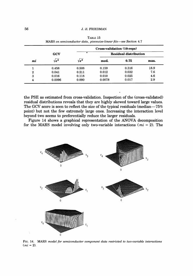
TABLE15 MARS on semiconductor data, piecewise-linear fits-see Section 4.7
Cross-validation (10-reps)
GCV I) Residual distribution
mi @ @ med. 0.75 max.
the PSE as estimated from cross-validation. Inspection of the (cross-validated) residual distributions reveals that they are highly skewed toward large values. The GCV score is seen to reflect the size of the typical residuals (median-75% point) but not the few extremely large ones. Increasing the interaction level beyond two seems to preferentially reduce the larger residuals.
Figure 14 shows a graphical representation of the ANOVA decomposition for the MARS model involving only two-variable interactions (mi = 2). The
FIG.14. MARS model for semiconductor component data restricted to two-variable interactions ( m i = 2).

MULTIVARIATE ADAPTIVE REGRESSION SPLINES
max = 1.0
max = ,065 max = .19
FIG.15. Full ( m i = 4) MARS model for semiconductor component data. Functions of V , and V, along various slices defined by V3and Vq.
resistor is seen to be a very nonlinear devick. The current appears to be roughly independent of the terminal voltages except when one or more of them take on extreme values where the current changes rapidly.
As seen in Table 15, the MARS model involving four-variable interactions provides a substantially better fit to these data. Figures 15 and 16 explore this function of four variables using the slicing strategy described before. Figure 15 shows the current as a function of Vl and V, along four slices defined by V3 and V,. In this figure, the functions are not plotted on the same vertical scale. In order to relate the scales, the maximum value of each function relative to that of the first (upper left frame) is shown above each plot. Since the relative locations of the plots are arbitrary, they are each plotted to have a minimum value of zero, so that the maximum value is equal to the range. The (V3, V,) slices are taken at the four extreme corners of the V3 - V, design. Both the magnitude and shape of the dependence of the current on Vl and V, are seen to depend rather strongly on the values of V3 and V,. For simultaneously low values of V3 and V, (upper left), the dependence is seen to be roughly linear, whereas when V, takes on its highest value, with V3 at its lowest value (lower left), the current is seen to vary much less as a function of V, and V,. For high values of V3, the dependence is similar to that of the lower left frame except for the existence of the dramatic peak for low values of V,.

J.H. FRIEDMAN
FIG.16. Full ( m i = 4) MARS model for semiconductor component data. Functions of V3and V4 along several slices defined by V, and V,.
Figure 16 shows the dependence of the current (as reflected by the MARS fit) on V3 and V, for four slices on (V,, V,). Here the slices do not include the two extreme corners on V, for low values of V2 since they are outside the support of the design. (This can be seen on the V1 - V2 plots; the functions are plotted only within the convex hull of the bivariate distributions.) In Figure 16, the functions are all plotted on the same scale. As would be expected from the previous results, the dependence of the current on V3 and V, changes substantially with differing values of V, and V,.
Exploring the resulting MARS model in this manner provides some insight into the nature of the cross-validated residual distributions observed in Table 15. The function has very high (and increasing) first and second derivatives very near some of the (joint) boundaries. When extreme observations on these boundaries are deleted during the cross-validation, the resulting slopes are underestimated and the extrapolation to the left-out observation gives rise to a large error. This phenomenon also explains why the piecewise-linear models give rise to much better fits. There are clearly small local regions where the second derivatives are very large. By approximating these by infinite second derivatives, the piecewise-linear model is able to come closer than the piece- wise-cubic fit which tries to moderate these locally very high second deriva- tives.
Figures 15 and 16 represent a small subset of all possible revealing slices of this four-variable function. In general, slicing is likely to be most effective when performed in an interactive manner. Functional dependencies revealed by inspecting the results of a particular slice will likely suggest further slices to try. The straightforward and rapid calculation of sliced models (72) from the
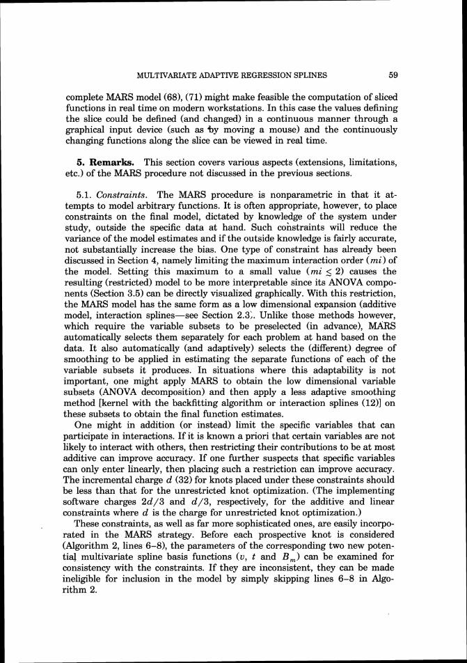
59 MULTIVARIATE ADAPTIVE REGRESSION SPLINES
complete MARS model (681, (71) might make feasible the computation of sliced functions in real time on modern workstations. In this case the values defining the slice could be defined (and changed) in a continuous manner through a graphical input device (such as %y moving a mouse) and the continuously changing functions along the slice can be viewed in real time.
5. Remarks. This section covers various aspects (extensions, limitations, etc.) of the MARS procedure not discussed in the previous sections.
5.1. Constraints. The MARS procedure is nonparametric in that it at- tempts to model arbitrary functions. It is often appropriate, however, to place constraints on the final model, dictated by knowledge of the system under study, outside the specific data at hand. Such cohstraints will reduce the variance of the model estimates and if the outside knowledge is fairly accurate, not substantially increase the bias. One type of constraint has already been discussed in Section 4, namely limiting the maximum interaction order (mi) of the model. Setting this maximum to a small value (mi _< 2) causes the resulting (restricted) model to be more interpretable since its ANOVA compo- nents (Section 3.5) can be directly visualized graphically. With this restriction, the MARS model has the same form as a low dimensional expansion (additive model, interaction splines-see Section 2.3;. Unlike those methods however, which require the variable subsets to be preselected (in advance), MARS automatically selects them separately for each problem at hand based on the data. I t also automatically (and adaptively) selects the (different) degree of smoothing to be applied in estimating the separate functions of each of the variable subsets it produces. In situations where this adaptability is not important, one might apply MARS to obtain the low dimensional variable subsets (ANOVA decomposition) and then apply a less adaptive smoothing method [kernel with the backfitting algorithm or interaction splines (12)l on these subsets to obtain the final function estimates.
One might in addition (or instead) limit the specific variables that can participate in interactions. If it is known a priori that certain variables are not likely to interact with others, then restricting their contributions to be at most additive can improve accuracy. If one further suspects that specific variables can only enter linearly, then placing such a restriction can improve accuracy. The incremental charge d (32) for knots placed under these constraints should be less than that for the unrestricted knot optimization. (The implementing software charges 2d/3 and d/3, respectively, for the additive and linear constraints where d is the charge for unrestricted knot optimization.)
These constraints, as well as far more sophisticated ones, are easily incorpo- rated in the MARS strategy. Before each prospective knot is considered (Algorithm 2, lines 6-81, the parameters of the corresponding two new poten- t i 4 multivariate spline basis functions (v, t and B,) can be examined for consistency with the constraints. If they are inconsistent, they can be made ineligible for inclusion in the model by simply skipping lines 6-8 in Algo- rithm 2.

60 J.H. FRIEDMAN
5.2. Semiparametric modeling. Another kind of a priori knowledge that is sometimes available has to do with the nature of the dependence of the response on some (or all) the predictor variables. The user may be able to provide a function g(x) that i ~ ~ t h o u g h t to capture some aspects of the true underlying function f(x). More generally, one may have a set of such func- tions {gj(x));', each one of which might capture some special aspect of the functional relationship. A semiparametric model of the form
where {(x) takes the form of the MARS approximation, could then be fit to the data. The coefficients c j in (73) are jointly fit along'with the parameters of the MARS model in Algorithms 2 and 3. To the extent that one or more of the gj successfully describe attributes of the true underlying function, they will be included with relatively large (absolute) coefficients and the accuracy of the resulting (combined) model will be improved.
Semiparametric models of this type (73) are easily fit using the MARS strategy. One simply includes {gj(x));! as J additional predictor variables ( x ,+~ ,. . . ,x , + ~ ) and constrains their contributions to be linear. One could also, of course, not place this constraint, thereby fitting more complex semi- parametric models than (73).
Another strategy that is often employed in this context is to first fit only the parametric component to the data and then apply a nonparametric method (such as MARS) to the residuals of the parametric fit. In general, this strategy is likely to be less successful because the residual function may be more highly structured than the original one (and thus more difficult to approximate) especially if the parametric approximation is not close to the true underlying function. The more general approach (73) allows the fitting procedure to automatically adjust the strength of the parametric components as part of the fitting process.
5.3. Collinearity. Extreme collinearity of the predictor variables is a fun- damental problem in the modeling of observational data. Solely in terms of predictive modeling, it represents an advantage in that it effectively reduces the dimensionality of the predictor variable space. This is only true provided that the observed collinearity is a property of the population distribution and not an artifact of the sample at hand. Collinearity presents, on the other hand, severe problems for interpreting the resulting model.
This problem is even more serious for (interactive) MARS modeling than for additive or linear modeling. Not only is it difficult to isolate the separate contributions of highly collinear predictor variables to the functional depen- dence, it is also difficult to separate the additive and interactive contributions among them. A highly nonlinear dependence on one such (highly correlated) variable can be well-approximated by a combination of functions of several of them and/or by interactions among them.

MULTIVARIATE ADAPTIVE REGRESSION SPLINES 61
In the context of MARS modeling, one strategy to cope with this (added) problem is to fit a sequence of models with increasing maximum interaction order (mi). One first fits an additive model (mi = I), then one that permits at most two variable interactions (mi = 2) and so on. The models in this se- quence can then be compared by means of their respective optimizing GCV scores. The one with the lowest mi value that gives a (relatively) acceptable fit can then be chosen.
Another (complementary) strategy is to directly resolve the ambiguity by enforcing parsimony on the number of variables that enter the model [Friedman and Silverman (1989)l. This will discourage spurious interaction effects caused by collinearity (or concurvity) and, in addition, partially stabilize the function estimates. I t will also aid in interpretation in that the resulting approximation will involve fewer variables.
Variable parsimony can be accomplished by introducing a small incremental penalty to the lack-of-fit criterion for choosing factors (knots) that involve introducing a new variable (not already in the model) as part of the forward stepwise procedure (Algorithm 2, line 7):
At the Mth iteration, there are M - 1basis functions currently in the model and the indicator function in (74) will be zero if the uth variable appears in at least one of them; otherwise it will be equal to one. The parameter y (> 0) regulates the strength of the penalty for entering new variables and can be used to control the lack-of-fit/variable parsimony tradeoff. Note that this penalty (74) is only introduced as part of the (forward stepwise) knot selection process and it is not used to reflect the overall lack-of-fit of the model.
In highly collinear settings the (unmodified) lack-of-fit criterion (LOF(g)) has very little preference on which particular variable to enter from a highly correlated set and a small value for y will cause the modified criterion (74) to repeatedly enter the same one from that set, without seriously degrading the quality of the approximation. A good value for y depends on the particular situation (degree of collinearity) and how much goodness-of-fit the user is willing to sacrifice for variable parsimony. This can be judged by examining the resulting fit quality for several (increasing) values of y as reflected by either the final GCV score (30) or a sample reuse method.
We illustrate these two approaches on data taken from the Places Rated Almanac [Boyer and Savageau (198611. They rated 329 American cities on the nine criteria listed in Table 16. For this exercise we attempt to model housing cost (y = x2)on the other eight criteria. Table 17 shows the resulting number of variables and GCV estimate (30) of the PSE (59) for running MARS with different values of y (74). The first three rows are for additive modeling (mi = 1) and the second three for models with two variable interactions permitted (mi = 2). The models involving interactions are seen to not be distinctly superior to the additive ones, so that using the first strategy (shown

TABLE16 The nine criteria used to rate U.S. cities by the Places Rated Almanac
climate housing costs
d
health care and environment crime rate transportation education access t o the arts recreational opportunities economics
earlier) one would be inclined to choose the latter. As the value of y (74) is steadily increased, MARS produces models with progressively fewer variables, as one would expect. For these particular data, however, one is able to reduce the number of variables from (nearly) the full set (at y = 0) to only three (0.05 Iy < 0.15) without seriously degrading the quality of the fit as esti- mated by the solution GCV score. Note that this GCV score (30) does not reflect the additional penalty imposed by setting y > 0, so that differences between scores involving larger and smaller values of y underestimate (on average) their actual differences. Ordinary cross-validation (CV) does account for this increased penalty. For example, the CV estimate (10 replications) for the y = 0 (mi = 1) model is 0.56 whereas the corresponding score for y = 0.1 is 0.52.
Figure 17 shows the graphical ANOVA decomposition for the three-variable additive model produced for 0.05 Iy < 0.15. From this analysis it appears that average (increasing) housing costs are most strongly affected by increas- ingly good climate (especially for the highest values) and are associated to a somewhat lesser degree with economic conditions and access to the arts. The dependence on climate might be somewhat surprising since in these data housing costs reflect utility bills, which are likely to decrease with good climate, as well as taxes and mortgage payments. Any interpretations, how-
TABLE17 The number of variables and corresponding GCV score for a sequence of MARS models on the
Placed Rated data, produced by increasing thepenalty y (74) for adding variables
m i = 1 Y 0 0.01 0.02 0.03 0.05 0.10 0.15 #vars 7 7 7 4 3 3 2 GCV 0.49 0.49 0.49 0.50 0.51 0.51 0.58
mi = 2 Y 0 0.01 0.02 0.05 0.07 0.10 0.15 #vars 8 6 5 5 4 3 2 GCV 0.48 0.50 0.48 0.47 0.51 0.51 0.58

MULTIVARIATE ADAPTIVE REGRESSION SPLINES
climate the arts
economics
FIG.17. Graphical ANOVA decomposition of the three variable additive MARS model on the Places Rated data, Section 5.3.
ever, must be tempered by the existence of the collinearities present in the design and the fact that the model is estimated to account for only 50% of the variance of the response.
5.4. Robustness. Since the MARS method as described here uses a model selection criterion based on squared-error loss, it is not robust against outlying response values. There is nothing fundamental about squared-error loss in the MARS approach. Any criterion can be used to select the multivariate spline basis functions, and construct the final fit, by simply replacing the internal linear least squares fitting routine (LOF-Algorithm 2, line 7 and Algorithm 3, lines 2 and 5) by one that minimizes another loss criterion (given the current set of multivariate spline basis functions). Using robust/resistant linear re- gression methods would provide resistance to outliers. The only advantage to squared-error loss in the MARS context is computational. It is difficult to see how rapid updating formulae (Section 3.9) could be developed for other types of linear regression.

64 J.H. FRIEDMAN
Gross outliers (in both the response and covariates) that can be detected through a preliminary (exploratory) analysis of the data, should be considered for removal before applying MARS. The MARS procedure is less sensitive than linear regression to covariate outliers owing to the local nature of the fit; sample covariate vectors far from an evaluation point tend to have less rather than more influence on the model estimate. Covariate outliers can have a strong influence on the fit near the corresponding data boundaries. This can be quite helpful if the corresponding response values for the outliers are correctly measured. If not, these outliers will contribute to end effect errors.
Recursive partitioning responds to outlying respcnse values by trying to isolate them. It produces a series of splits so as to place each such outlier in its own region. This localizes the effect of the outlier(s) so that they only distort the fit for covariate values close to that of the outlier(s). The MARS procedure operates similarly. It will also try to isolate outliers through a series of corresponding splits producing basis functions that attempt to capture the (apparent) high curvature of the function near each outlier. The outliers will tend to heavily influence the values of the coefficients of their corresponding basis functions, but have much less influence on the rest of the fit. The particular basis functions introduced in this manner by outlying response values may tend to involve interactions of high order depending on their location in the covariate space. Thus, interpreting the presence of interaction effects can be highly distorted by the existence of outlying response values.
Computationally feasible methods of robustifying the MARS procedure are currently under investigation.
6. Conclusion. The aim of the MARS procedure is to combine recursive partitioning and spline fitting in a way that best retains the positive aspects of both, while being less vulnerable to their unfavorable properties. This has been accomplished, at least to some extent. The greatest strength of recursive partitioning is its adaptability, through its local variable subset selection strategy. This makes it a highly dynamic computation (Section 2.4) capable of tracking the dependencies associated with a wide variety of complex functional forms. The two weaknesses of recursive partitioning are the lack of continuity of its models and its inability to capture simple relationships such as linear, additive or interactions of low order compared to n . Nonadaptive (tensor product) spline fitting produces continuous models with continuous deriva- tives. I t strongly suffers, however, from the curse-of-dimensionality in that very large basis function sets are usually required in high dimensions to capture relatively simple functional relationships.
The MARS procedure completely retains the adaptability of recursive parti- tioning by its close adherence to the recursive splitting paradigm (compare Algorithms 1 and 2). It is in fact much more adaptive because it permits the recursive splitting of all basis functions (nodes) in the model and not just those that are currently terminal. This causes it to overcome the second problem (mentioned in the previous paragraph) associated with recursive partitioning. I t produces continuous models by replacing the step functions (19), (20) by

65 MULTIVARIATE ADAPTIVE REGRESSION SPLINES
q = 1truncated power spline basis functions (211, (22). Continuous derivatives are obtained through the strategy outlined in Section 3.7. From the point of view of tensor product spline methods, MARS can be viewed as a hierarchical forward/backward stepwise subset: selection procedure for choosing a subbasis appropriate for the problem at hand, from the complete (q = 1) truncated power tensor product basis with knots at every (distinct) marginal data value. MARS models have a fair degree of interpretability through the ANOVA decomposition (Section 3.5) that breaks up the approximation into an additive component and into interaction contributions of various orders.
Slicing (Section 4.7) can be used to explore the higher dimensional aspects of the models.
The implementation of the adaptive regression spline strategy presented here represents a first attelzpt in that particular 'choices have been made concerning many of the engineering details in the absence of a great deal of experience with the procedure. Although incidental to the fundamental ideas, these details can have a strong bearing on performance. As experience is gained, it is likely that many of the choices taken here will be seen to be less than optimal and suitable modifications will emerge that improve the perfor- mance of the procedure. The attempt here has been to demonstrate that the adaptive regression spline strategy, first introduced by Smith (1982) (in the univariate setting), holds substantial promise as a tool for multivariate func- tion estimation.
A FORTRAN program implementing the MARS procedure is available from the author.
Acknowledgments. Helpful discussions with Terry Therneau are grate- fully acknowledged. The author is grateful to Kishore Singhal for providing the semiconductor test data used in Section 4.7.
REFERENCES
ANDREWS, A. M. (1985). Data. A Collection of Problems for Many Fields for D. F . and HERZBERG, the Student and Research Worker. Springer, New York.
BARRY,D. (1986). Nonparametric Bayesian regression. Ann Statist. 14 934-953. BELLMAN,R. E. (1961). Adaptive Control Processes. Princeton Univ. Press. BOYER, R. and SAVAGEAU, D. (1986). Places Rated Almanac. Rand McNally. BOZZINI, L. (1985). Local smoothing for scattered noisy data. Internat. Ser. M. and LENARDUZZI,
Numer. Math. 75 51-60. Birkhauser, Basel. BREIMAN, J . H. (1985). Estimating optimal transformations for multiple regres- L. and FRIEDMAN,
sion and correlation (with discussion). J.Amer. Statist. Assoc. 80 580-619. BREIMAN,L., FRIEDMAN, R. A. and STONE, J . H., OLSHEN, C. J . (1984). Classification and Regres-
sion Trees. Wadsworth, Belmont, Calif. BREIMAN,L. and MEISEL, W . S. (1976). General estimates o f the intrinsic variability o f data in
nonlinear regression models. J . Amer. Statist. Assoc. 71 301-307. BREIMAN, L. and PETERS, S. (1988). Comparing automatic bivariate smoothers (a public service
enterprise). Technical Report 161, Dept. Statist., Univ. Calif., Berkeley. BROUNCKER,LORD (1734). Experiments o f the recoiling o f guns. In The History of the Royal
Society of London, 4 th ed. 233-239.

66 J . H. FRIEDMAN
BUJA, A., HASTIE, T. and TIBSHIRANI, R. (1989). Linear smoothers and additive models (with discussion). Ann. Statist. 17 453-555.
CHEN,Z., Gu, C. and WAHBA, G. (1989). Comment on "Linear smoothers and additive models," by Buja. Hastie and Tibshirani. Ann. Statist. 17 515-521.
CLEVELAND, S. (1979). Robust focally weighted regression and smoothing scatter plots.W. J . Amer. Statist. Assoc. 74 828-836.
CLEVELAND, S. J . (1988). Locally weighted regression: An approach to regres- W. S, and DEVLIN, sion analysis by local fitting. J . Amer. Statist. Assoc. 83 596-610.
COPAS, J . B. (1983). Regression prediction and shrinkage (with discussion). J. Roy. Statist. Soc. Ser. B 45 311-354.
Cox, D. R. (1970). Analysis of Binary Data. Chapman and Hall, London. CRAVEN,P. and WAHBA, G. (1979). Smoothing noisy data with spline functions. Estimating the
correct degree of smoothing by the method of generalized cross-validation. Numer. Math. 31 317-403.
DE BOOR, C. (1978). A Practical Guide to Splines. Springer, New York. DIACONIS, M. (1984). On nonlinear functions of linear combinations. SIAMP. and SHAHSHAHANI,
J . Sci. Statist. Comput. 5 175-191. DONGARRA,J. J. , MOLER, C. B., BUNCH, J. R. and STEWART, G. W. (1979). Linpack Users' Guide.
SIAM, Philadelphia. DONOHO,D. L. and JOHNSTONE, and a duality with I. (1989). Projection-based approximation
kernel methods. Ann. Statist. 17 58-106. EFRON,B. (1983). Estimating the error rate of a prediction rule: Improvement on cross-validation.
J . Amer. Statist. Assoc. 78 316-331. FORINA,M., ARMANINO, S., CALCAGNO, E. (1983). Evaluation of the C., LANTERI, C, and TISCORNIA,
chemical characteristics of olive oils as a function of production year by multivariate methods. La Revista Italiana delle Sostanze Grasse 60.
FRIEDMAN,J . H. (1979). A tree-structured approach to nonparametric multiple regression. In Smoothing Techniques for Curve Estimation (T. H. Gasser and M. Rosenblatt, eds.) 5-22. Springer, New York.
FRIEDMAN,J. H. (1985). Classification and mv.ltiple response regression through projection pur- suit. Technical Report LCSO12, Dept. Statist., Stanford Univ.
FRIEDMAN,J . H. (1988). Fitting functions to noisy data in high dimensions. In Computing Science and Statistics: Proc. Twentieth Symp. on the Interface (E. J . Wegman, D. T. Gantz and J. J. Miller, eds.) 13-43. Amer. Statist. Assoc., Alexandria, Va.
FRIEDMAN, W. (1983). Multidimensional additive spline approxi- J . H., GROSSE, E. and STUETZLE, mation. SIAM J . Sci. Statist. Comput. 4 291-301.
FRIEDMAN, B. W. (1989). Flexible parsimonious smoothing and additive J . H. and SILVERMAN, modeling. Technometrics 31 3-39.
FRIEDMAN, W. (1981). Projection pursuit regression. J . Amer. Statist. Assoc. J . H. and STUETZLE, 76 817-823.
FRIEDMAN,J. H. and WRIGHT, M. H. (1981). A nested partitioning procedure for numerical multiple integration. ACM Trans. Math. Software 7 76-92.
GOLUB,G. H. and VAN LOAN, C. F. (1983). Matrix Computations. The Johns Hopkins Univ. Press, Baltimore.
Gu, C., BATES, D. M., CHEN, Z. and WAHBA, G. (1990). The computation of GCV function through Householder tridiagonalization with application to the fitting of interaction spline models. SIAM J . Matrix Anal. 10 457-480.
Gu, C. and WAHBA, G. (1991). Minimizing GCV/GML scores with multiple smoothing parameters via the Newton method. SIAM J . Sci. Statist. Comput. 12.
HASTIE,T . and TIBSHIRANI, R. (1986). Generalized additive models (with discussion). Statist. Sci. 1 297-318.
HUBER,P. J . (1985). Projection pursuit (with discussion). Ann. Statist. 13 435-475. LYNESS, J . N. (1970). Algorithm 379-SQUANK (Simson Quadrature Used Adaptively-Noise
Killed). Comm. ACM 13 260-263.

67 MULTIVARIATE ADAPTIVE REGRESSION SPLINES
MORGAN,J. N. and SONQUIST, J. A. (1963). Problems in the analysis of survey data, and a proposal. J . Amer. Statist. Assoc. 58 415-434.
PARZEN,E. (1962). On estimation of a probability density function and mode. Ann. Math. Statist. 33 1065-1076.
SHEPARD,D. (1964). A two-dimensional ihterpolation function for irregularly spaced data. Proc. 1964 ACM Nat. Conf. 517-524.
SHUMAKER,L. L. (1976). Fitting surfaces to scattered data. In Approximation Theory II (G. G. Lorentz, C. K. Chui and L. L. Shumaker, eds.) 203-268. Academic, New York.
SHUMAKER, L. L. (1984). On spaces of piecewise polynomials in two variables. In Approximation Theory and Spline Functions (S. P. Singh, J. H. W. Barry and B. Watson, eds.) 151-197. Reidel, Dordrecht, Holland.
SILVERMAN,B. W. (1985). Some aspects of the spline smoothing approach to nonparametric regression curve fitting. J . Roy. Statist. Soc. Ser. B 47 1-52.
SMITH, P. L. (1982). Curve fitting and modeling with splines using statistical variable selection techniques. Report NASA 166034, Langley Research Center, Hampton, Va.
STONE, C. J. (1977). Nonparametric regression and its applications (with discussion). Ann. Statist. 5 595-645.
STONE, C. J. and Koo, C.-Y. (1985). Additive splines in statistics. Proc. Ann. Meeting Amer. Statist. Assoc. Statist. Comp. Section 45-48.
STONE,M . (1974). Cross-validatory choice and assessment of statistical predictors (with discus- sion). J . Roy. Statist. Soc. ser . B 36 111-147.
WAHBA,G. (1986). Partial and interaction splines for the semiparametric estimation of functions of several variables. In Computer Science and Statistics: Proc. Eighteenth Symp. on the Interface (T. J . Boardman, ed.) 75-80. Amer. Statist. Assoc., Alexandria, Va.
WAHBA,G. (1990). Spline Models for Observational Data. SIAM, Philadelphia.
DISCUSSION
University of Illinois
1. Introduction. We describe the multivariate adaptive polynomial syn- thesis (MAPS) method of multivariate nonparametric regression and compare it to the multivariate adaptive regression spline (MARS) method of Friedman (1990). Both MAPS and MARS are specializations of a general multivariate regression algorithm that builds hierarchical models using a set of basis functions and stepwise selection. We compare polynomial and spline bases in this context. Our experience is that there is no substantial difference in the statistical accuracy for the data sets that we have investigated, provided that some care is taken in the choice of the model selection criterion. I t is argued that the polynomial methods, with a smaller set of basis functions to select from at each step, should yield a computationally faster algorithm.