Multistability and the control of complexityUlrike Feudel and Celso Grebogi

Citation: Chaos: An Interdisciplinary Journal of Nonlinear Science 7, 597 (1997); doi: 10.1063/1.166259 View online: http://dx.doi.org/10.1063/1.166259 View Table of Contents: http://scitation.aip.org/content/aip/journal/chaos/7/4?ver=pdfcov Published by the AIP Publishing Articles you may be interested in Chaotification of complex networks with impulsive control Chaos 22, 023137 (2012); 10.1063/1.4729136 Simple driven chaotic oscillators with complex variables Chaos 19, 013124 (2009); 10.1063/1.3080193 Control of implicit chaotic maps using nonlinear approximations Chaos 10, 676 (2000); 10.1063/1.1288149 Complex motion of Brownian particles with energy supply AIP Conf. Proc. 502, 183 (2000); 10.1063/1.1302383 Stability analysis of fixed points via chaos control Chaos 7, 590 (1997); 10.1063/1.166258

This article is copyrighted as indicated in the article. Reuse of AIP content is subject to the terms at: http://scitation.aip.org/termsconditions. Downloaded to IP: 158.39.37.3

On: Wed, 02 Apr 2014 08:37:30

This article i

Multistability and the control of complexityUlrike Feudel and Celso Grebogia)

Institut fur Physik, Universita¨t Potsdam, PF 601553, D–14415 Potsdam, Germany

~Received 5 May 1997; accepted for publication 4 August 1997!

We show how multistability arises in nonlinear dynamics and discuss the properties of such abehavior. In particular, we show that most attractors are periodic in multistable systems, meaningthat chaotic attractors are rare in such systems. After arguing that multistable systems have thegeneral traits expected from a complex system, we pass to control them. Our controlling complexityideas allow for both the stabilization and destabilization of any one of the coexisting states. Thecontrol of complexity differs from the standard control of chaos approach, an approach that makesuse of the unstable periodic orbits embedded in an extended chaotic attractor. ©1997 AmericanInstitute of Physics.@S1054-1500~97!01004-5#

--

s

-

ntesellt

isas-

era

nlteriestaetha

the

inients

ghlyn-if-

ofoise,ilizesryors.

ofann-dhenotic

dicen-

tingbutbe-i-

nyandowov-ardiesthe

ofureson-reeical

lan

The study of nonlinear systems has yielded many richand varied dynamics. While the behavior of low-dimensional systems, where only one or two attractorsdominate the system’s dynamics has been studied intensively, much less is known about systems where a multitude of attractors coexist for a given set of parameters.Physical systems known to exhibit such multistable be-havior have been found in diverse areas of the naturalsciences such as condensed matter physics, laser opticreaction-diffusion systems, and neuronal dynamics. Inthis paper, we study the global dynamics of a system having a large number of coexisting attractors and show howa small amount of noise can influence the behavior of thesystem and result in complex dynamics. We then showthat small perturbations allow us to control and manipu-late the system’s complexity.

I. INTRODUCTION

Many processes in nature do not possess only one loterm asymptotic state or attractor, but are rather characized by a large number of coexisting attractors for a fixedof parameters. This implies that which attractor is eventuareached by a trajectory of the system depends strongly oninitial condition. This phenomenon, called multistability,found commonly in many fields of science suchneuroscience,1,2 chemistry,3–5 optics,6,7 and condensed matter physics.8

What makes many multistable systems particularly intesting are their ability to exhibit a multitude of attractors, sover 100 or even over 1000 coexisting attractors.9,10 In facttheir dynamics is characterized by a lot of attractors, maiperiodic ones, each having a rather complicatedly intwined basin structure. Moreover, the basin boundaamong all these periodic attractors permeate most of thespace, except for small open neighborhoods about the podic attractors, and their dimensions are very close todimension of the state space. Since most of the attractors

a!Permanent address: Institute for Plasma Research, University of MaryCollege Park, Maryland 20742.

Chaos 7 (4), 1997 1054-1500/97/7(4)/597/8/$10.00s copyrighted as indicated in the article. Reuse of AIP content is subject to

On: Wed, 02 Apr

,

g-r-t

yhe

-y

yr-steri-ere

periodic, the chaotic component of the dynamics is inchaotic saddles embedded in the basin boundary.11 As a re-sult, trajectories, starting with arbitrary initial conditionsthe state space, experience periods of long chaotic transbefore approaching one of the periodic attractors.10,12 There-fore, because of these chaotic saddles, the trajectory is hisensitive to the final state. A slight change in the initial codition results in a trajectory that is attracted to a totally dferent periodic orbit.

Such a system is highly sensitive to small amountsnoise in the sense that the presence of small amplitude ntypical in so many natural processes, is enough to destabthe periodic behavior.12 It means that a typical orbit bouncechaotically for long time in the massive basin boundastructure before cascading into one of the periodic attractOnce there, the trajectory remains in the neighborhoodthis particular periodic attractor for some time executingalmost periodic motion until the right amount of noise evetually moves the orbit out of this ‘‘metastable’’ state anback into the fractal basin boundary region. One can say tthat the orbit alternates between epochs of random or chamotion and epochs of coherent or almost periomotion.12–14 Such a behavior has been observed experimtally in Rayleigh–Be´nard convection,15 in coupled lasersystems,16,17 and in fluidized beds.18

Such a complex dynamics, the coexistence of compebehaviors on which the trajectory alternates, is peculiar,not necessarily, to higher dimensional systems. Whichhavior is observed at a given time is highly sensitive to mnor perturbations. The two attributes, accessibility to mastates and sensitivity, allows us to influence, manipulate,control the dynamics of such a complex system. Unlike ldimensional chaotic systems in which the dynamics is gerned by a single large attractor and in which the standideas19 on controlling chaos can be applied, new possibilitarise, as it will be discussed here, when dealing withcontrol of complex systems.12

The purpose of this paper is to study the behaviormultistable systems. In Sec. II, we describe the basic featof multistable systems, systems that are obtained from cservative ones by adding a small amount of damping. Thsystems are considered for their importance in dynamd,

597© 1997 American Institute of Physicsthe terms at: http://scitation.aip.org/termsconditions. Downloaded to IP: 158.39.37.3

2014 08:37:30

sAnyssrr

ate

siduracthtoea

cocaflerythdis

daaishMn

osrb

tr

tivdarit.

andis

hendzeysntf

a-

Itthepa-be

alach

ur-ul-

on-ofis

erit

e

x isrilene

s of

ityop-

598 U. Feudel and C. Grebogi: Multistability and the control of complexity

This article i

systems: The kicked single rotor, the He´non map, and theoptical cavity map. In spite of their particular differencetheir general features regarding multistability are similar.important question arising from the study of multistable stems is how prevalent chaotic attractors are. Investigationthe kicked single rotor show that, among the large numbeattractors coexisting for a given set of parameters, none omost very few are chaotic. In fact, we find that chaotictractors occur only in very tiny intervals in parameter spac9

We find the same behavior to hold for every system conered in this paper. Therefore, in Sec. III, we present measfor the extension of the chaotic region in parameter spand their scaling with the damping. We also argue thatrelative size of the basin of attraction of a particular attracdecreases as the extension of the chaotic region in paramspace decreases. Finally, in Sec. IV, a control strategyplied to multistable systems is discussed. Based on thetrol objectives, we show that different metastable statesbe stabilized. We also show that we can use the sameibility offered by multistable systems to allow the trajectoto access only certain metastable states while avoiding oparticular ones. In every case a feedback control is usemanipulate the multistable system both either without noor under the influence of noise.

II. WEAKLY DISSIPATIVE SYSTEMS POSSESSINGMULTISTABILITY

The easiest way to construct a multistable system istake a conservative one and introduce small amounts ofsipation. Dynamically it happens in the following way. Inconservative system, where the modulus of the determinof the Jacobian matrix for a map is equal to 1, we distingutwo different types of dynamics, regular and chaotic. Tregular behavior occurs in the KAM islands and in the KAtori, which are embedded in the chaotic sea. These islaare associated with marginally stable periodic orbits wheigenvalues are equal to one in absolute value. The laones, the so-called primary islands, are surroundedsmaller secondary islands. This classification has been induced in Hamiltonian theory.20 If a small amount of dampingis added to such a system, one gets a family of dissipadynamical systems in which these marginally stable perioorbits turn into periodic attractors whose eigenvaluessmaller than one in absolute value. But instead of an infinnumber of attractors we find only a finite number of them9

How large this number is, depends on the damping levelthe particular family under consideration. Every KAM islanis converted into an attractor and such an attractor exeven for large damping.21 But one needs larger ‘‘forcing’’ or‘‘nonlinearity’’ to have it.

There is one family of dynamical systems, in which tnumber of attractors associated with the primary islascales as 1/damping, i.e., when the damping tends totheir number tends to infinity. The related conservative stem possesses primary islands corresponding to an efamily of periodic orbits. An example of such a family o

Chaos, Vol. 7,s copyrighted as indicated in the article. Reuse of AIP content is subject to

On: Wed, 02 Apr

,

-ofofat-.-eseerterp-n-nx-

ertoe

tois-

nthe

dsegeyo-

eicee

d

ts

sro-ire

systems is the periodically kicked single rotor, or equivlently, the dissipative standard map:

xn115xn1yn mod 2p,~1!

yn115~12n!yn1 f 0sin~xn1yn!.

The family can be parameterized by the dampingn and theforcing f 0. This family was analyzed in detail in Ref. 9.shows a highly multistable behavior as compared withfamilies of systems introduced next. Depending on therametersf 0 andn, the number of coexisting attractors canarbitrarily large.

On the other hand, there are other families of typicdynamical systems where the conservative element of efamily has one or, at most just a few, primary island srounded by secondary islands. These families also show mtistable behavior when small damping is added. But in ctrast with the previously mentioned family, the numbercoexisting attractors is much less. Two families with thkind of behavior are studied in this paper, the He´non andoptical cavity maps,6 both are well-known families.

We study the He´non map in the form:

xn115A2xn22~12n!yn ,

~2!yn115xn.

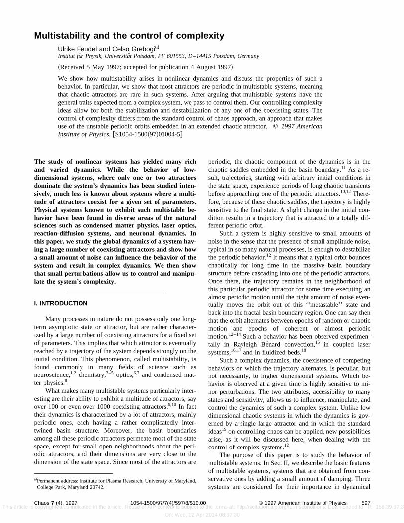
This system possesses two parameters. The parametn,which varies between 0 and 1, is the damping. In the limn51, the two equations in Eq.~2! are decoupled and ongets the quadratic map. In the other limit,n50 the map is nolonger dissipative, the determinant of the Jacobian matriequal to 1. The parameterA represents the bifurcation ocontrol parameter and it is the nonlinearity parameter. Whin the case of the quadratic map there exists only obounded attractor in a wide range of the parameterA, weargue that there are several coexisting attractors for valuen close to the no damping limitn50, as shown in Fig. 1.

The third map under consideration is the optical cavmap which describes the behavior of a laser pulse in antical cavity:6

FIG. 1. Bifurcation diagram for the He´non map~2! with n50.02.

No. 4, 1997the terms at: http://scitation.aip.org/termsconditions. Downloaded to IP: 158.39.37.3

2014 08:37:30

-e

avelec

g

eavr au

metears-

r.cicnte

sethmeruc

ritab

asini-ofacha

alWe

o-

ns

x-

ethe

rss

599U. Feudel and C. Grebogi: Multistability and the control of complexity

This article i

zn115I 1~12n!znexpS ik2ip

11uznu2D , ~3!

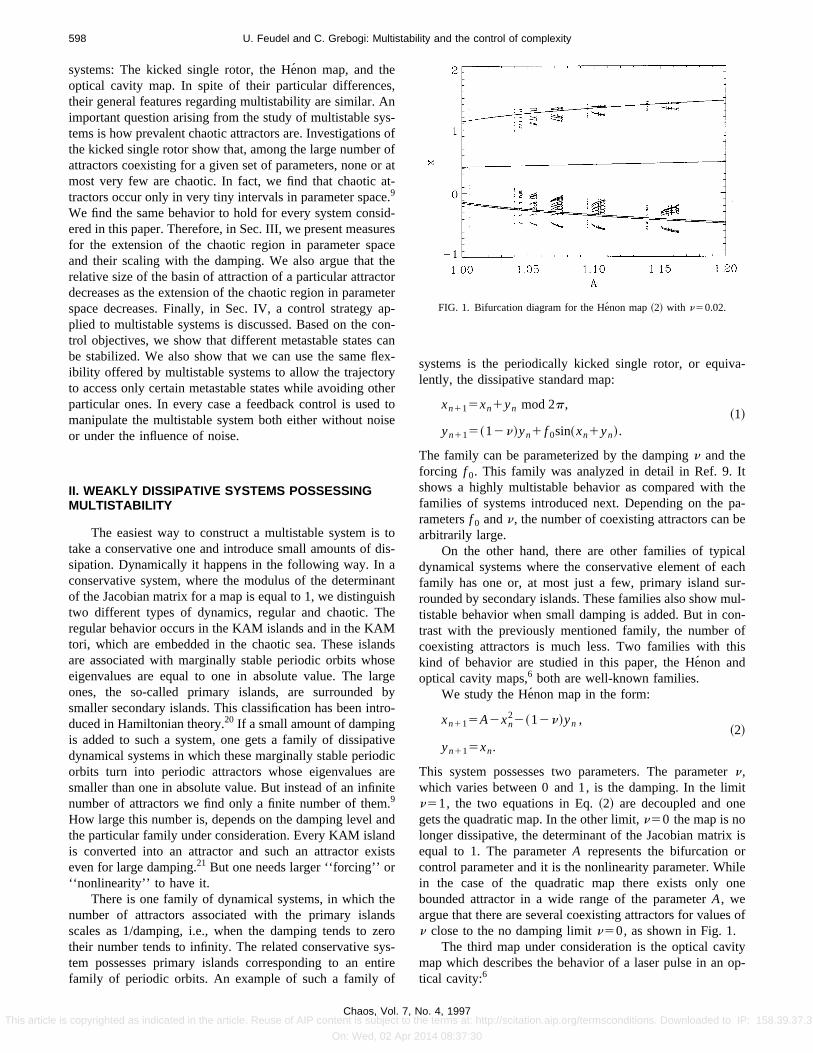
where zn is a complex quantityzn5xn1 iyn related to theamplitude and phase of then-th laser pulse exiting the cavity. The parameterI is related to the laser input amplitudand can thus be thought of as the forcing. The dampingn isrelated to the reflection properties of the mirrors in the city. The parameterk is the empty cavity detuning and thparameterp measures the detuning due to a nonlinear dietric medium. They are kept fixed atk50.4 and p53.5.Again we find intervals in parameter space correspondinmultistable behavior, as shown in Fig. 2.

There are general properties which are common to ththree multistable dynamical systems. Some of them hbeen first described in Ref. 9 using the kicked single rotoa prototype example. Similar properties have been also fofor the Henon map~2! and the optical cavity map~3!, asshown next.

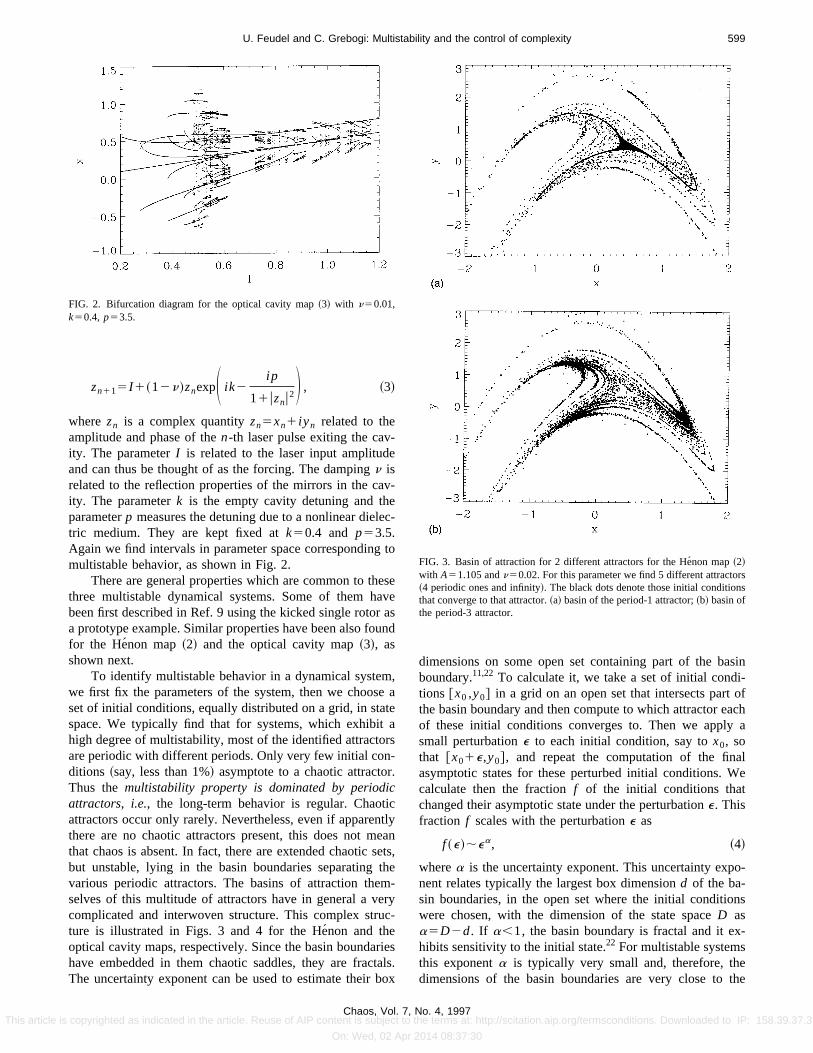
To identify multistable behavior in a dynamical systewe first fix the parameters of the system, then we choosset of initial conditions, equally distributed on a grid, in staspace. We typically find that for systems, which exhibithigh degree of multistability, most of the identified attractoare periodic with different periods. Only very few initial conditions ~say, less than 1%! asymptote to a chaotic attractoThus themultistability property is dominated by periodiattractors, i.e., the long-term behavior is regular. Chaotattractors occur only rarely. Nevertheless, even if apparethere are no chaotic attractors present, this does not mthat chaos is absent. In fact, there are extended chaoticbut unstable, lying in the basin boundaries separatingvarious periodic attractors. The basins of attraction theselves of this multitude of attractors have in general a vcomplicated and interwoven structure. This complex strture is illustrated in Figs. 3 and 4 for the He´non and theoptical cavity maps, respectively. Since the basin boundahave embedded in them chaotic saddles, they are fracThe uncertainty exponent can be used to estimate their

FIG. 2. Bifurcation diagram for the optical cavity map~3! with n50.01,k50.4, p53.5.

Chaos, Vol. 7,s copyrighted as indicated in the article. Reuse of AIP content is subject to

On: Wed, 02 Apr

-

-

to

sees

nd

,a

lyants,e-y-

esls.ox

dimensions on some open set containing part of the bboundary.11,22 To calculate it, we take a set of initial condtions @x0 ,y0# in a grid on an open set that intersects partthe basin boundary and then compute to which attractor eof these initial conditions converges to. Then we applysmall perturbatione to each initial condition, say tox0, sothat @x01e,y0#, and repeat the computation of the finasymptotic states for these perturbed initial conditions.calculate then the fractionf of the initial conditions thatchanged their asymptotic state under the perturbatione. Thisfraction f scales with the perturbatione as

f ~e!;ea, ~4!

wherea is the uncertainty exponent. This uncertainty expnent relates typically the largest box dimensiond of the ba-sin boundaries, in the open set where the initial conditiowere chosen, with the dimension of the state spaceD asa5D2d. If a,1, the basin boundary is fractal and it ehibits sensitivity to the initial state.22 For multistable systemsthis exponenta is typically very small and, therefore, thdimensions of the basin boundaries are very close to

FIG. 3. Basin of attraction for 2 different attractors for the He´non map~2!with A51.105 andn50.02. For this parameter we find 5 different attracto~4 periodic ones and infinity!. The black dots denote those initial conditionthat converge to that attractor.~a! basin of the period-1 attractor;~b! basin ofthe period-3 attractor.

No. 4, 1997the terms at: http://scitation.aip.org/termsconditions. Downloaded to IP: 158.39.37.3

2014 08:37:30

thF

siorth

ich

eaonto

nto

llIf

edihaotht tinise

ssia

ivait

re

itre

ns atall.

om-orsms,tiveltom-

o-

ins

theare

are

riesely

utsults

at-fur-non-ct

heeter

ng

ointum

sis,

, oftheaoss athestone bi-

gs

ap-

ityeditiath

600 U. Feudel and C. Grebogi: Multistability and the control of complexity

This article i

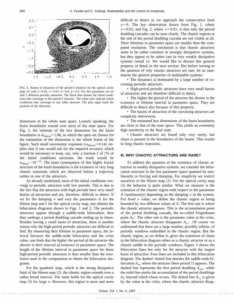
dimension of the whole state space. Loosely speaking,basin boundaries extend over most of the state space.Fig. 3, the estimate of the box dimension for the baboundaries isdHenon51.86, in which the open set chosen fthe estimation of the dimension is the whole frame offigure. Such small uncertainty exponent (aHenon50.14) im-plies that if one would ask for the required accuracy whwould be necessary to keep, say, only a fractionf of 1% ofthe initial conditions uncertain, the result would beHenon;10215. The main consequence of this highly fractstructure of the basin boundaries is the existence of very lchaotic transients which are observed before a trajecsettles in one of the attractors.

As already mentioned, most of the initial conditions coverge to periodic attractors with low periods. This is duethe fact that the attractors withhigh periods have very smabasins of attractionand are, therefore, difficult to detect.we fix the dampingn and vary the parametersA for theHenon map andI for the optical cavity map, one obtains thbifurcation diagrams shown in Figs. 1 and 2. The perioattractors appear through a saddle-node bifurcation, tthey undergo a period doubling cascade ending up in chBesides having a small basin of attraction, there is anoreason why the high-period periodic attractors are difficulfind. By measuring their lifetime in parameter space, theterval between the saddle-node bifurcation and the crvalue, one finds thatthe higher the period of the attractor thshorter is their interval of existence in parameter space. Thelength of the lifetime interval in parameter space for thohigh-period periodic attractors is thus smaller than the relution used in the computation to obtain the bifurcation dgrams.

For the quadratic map, which is the strong dissipatlimit of the Henon map~2!, the chaotic region extends overrather broad interval. The same holds for the optical cavmap ~3! for largen. However, this region is more and mo

FIG. 4. Basins of attraction of the period-3 attractor for the optical cavmap ~3! with I 50.45, n50.01, k50.4, p53.5. For this parameter set wfind 5 different periodic attractors. The black dots denote the initial contions that converge to the period-3 attractor. The white dots indicate inconditions that converge to any other attractor. The plus signs markposition of the attractors.

Chaos, Vol. 7,s copyrighted as indicated in the article. Reuse of AIP content is subject to

On: Wed, 02 Apr

eor

n

e

lg

ry

-

cens.

ero-is

eo--

e

y

difficult to detect as we approach the conservative limn50. The key observation drawn from Fig. 1, when50.02, and Fig. 2, wheren50.01, is that only the perioddoubling cascades can be seen clearly. The chaotic regiothe end of the period doubling cascade are not visible atTheir lifetimes in parameter space are smaller than the cputed resolution. The conclusion is that chaotic attractseem to be rather common in strongly dissipative systebut they appear to be rather rare in very weakly dissipasystems~small n). We would like to discuss this generaproperty in detail in the next section. But before turningthe question of why chaotic attractors are rare, let us sumarize the general properties of multistable systems:

• The dynamics is dominated by a large number of cexisting periodic attractors.

• High-period periodic attractors have very small basof attraction and are therefore difficult to detect.

• The higher the period of the attractor the shorter isexistence or lifetime interval in parameter space. Theydifficult to detect also because of this property.

• The basins of attraction of the coexisting attractorscomplexly interwoven.

• The estimated box dimensions of the basin boundaare close to that of the state space. This yields an extremhigh sensitivity to the final state.

• Chaotic attractors are found only very rarely, bchaos is present in the boundaries of the basins. This rein long chaotic transients.

III. WHY CHAOTIC ATTRACTORS ARE RARE?

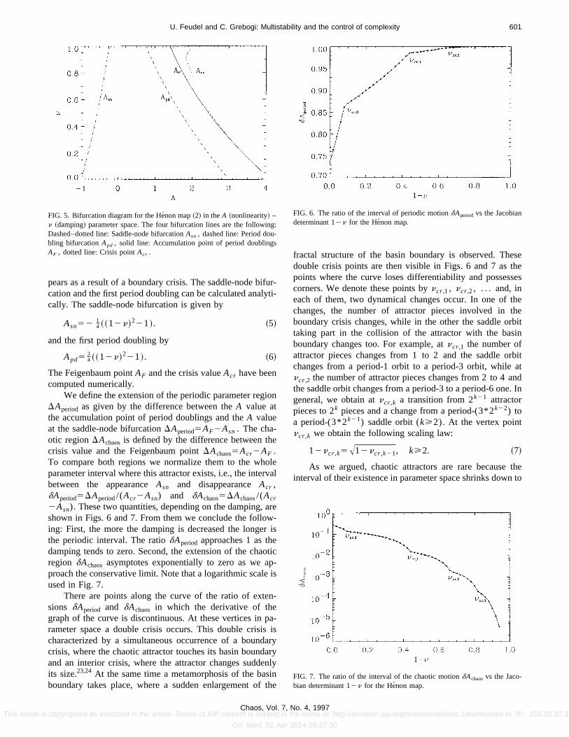
To address the question of the existence of chaotictractors in weakly dissipative systems, we consider the bication structure in the two parameter space spanned bylinearity or forcing and damping. For simplicity we restriourselves to the He´non map~2!. For the optical cavity map~3! the behavior is quite similar. What we measure is textension of the chaotic region with respect to the paramA ~nonlinearity! depending on the dampingn in the system.For fixed n value, we define the chaotic region as beibounded by two different values ofA. The first one is wherethe chaotic attractor appears. This is the accumulation pof the period doubling cascade, the so-called Feigenbapoint AF . The other one is the parameter value at the criwhere the chaotic attractor disappearsAcr . Of course weunderstand that there are a large number, possibly infiniteperiodic windows embedded in the chaotic region. Butchaotic region, as we define it, gives the extension of chin the bifurcation diagram either as a chaotic attractor or achaotic saddle in the periodic windows. Figure 5 showsbifurcation lines but only for the attractor with the largebasin of attraction. Four lines are included in this bifurcatidiagram. The dashed–dotted line denotes the saddle-nodfurcationAsn where the attractor~here period 1! appears. Thedashed line represents the first period doublingApd , whilethe solid line marks the accumulation of the period doublinAF beyond which chaos occurs. The dotted lineAcr is givenby the value at the crisis, where the chaotic attractor dis

i-le

No. 4, 1997the terms at: http://scitation.aip.org/termsconditions. Downloaded to IP: 158.39.37.3

2014 08:37:30

ifuly

io

e

olrv

awreop

e

n

paisdaa

ensif t

esetheses

thetherbitin

rbitat

and. In

then to

ng-s

601U. Feudel and C. Grebogi: Multistability and the control of complexity

This article i

pears as a result of a boundary crisis. The saddle-node bcation and the first period doubling can be calculated anacally. The saddle-node bifurcation is given by

Asn52 14 ~~12n!221!. ~5!

and the first period doubling by

Apd5 34 ~~12n!221!. ~6!

The Feigenbaum pointAF and the crisis valueAcr have beencomputed numerically.

We define the extension of the periodic parameter regDAperiod as given by the difference between theA value atthe accumulation point of period doublings and theA valueat the saddle-node bifurcationDAperiod5AF2Asn . The cha-otic regionDAchaosis defined by the difference between thcrisis value and the Feigenbaum pointDAchaos5Acr2AF .To compare both regions we normalize them to the whparameter interval where this attractor exists, i.e., the intebetween the appearanceAsn and disappearanceAcr ,dAperiod5DAperiod/(Acr2Asn) and dAchaos5DAchaos/(Acr

2Asn). These two quantities, depending on the damping,shown in Figs. 6 and 7. From them we conclude the folloing: First, the more the damping is decreased the longethe periodic interval. The ratiodAperiod approaches 1 as thdamping tends to zero. Second, the extension of the charegion dAchaos asymptotes exponentially to zero as we aproach the conservative limit. Note that a logarithmic scalused in Fig. 7.

There are points along the curve of the ratio of extesions dAperiod and dAchaos in which the derivative of thegraph of the curve is discontinuous. At these vertices inrameter space a double crisis occurs. This double crischaracterized by a simultaneous occurrence of a bouncrisis, where the chaotic attractor touches its basin boundand an interior crisis, where the attractor changes suddits size.23,24 At the same time a metamorphosis of the baboundary takes place, where a sudden enlargement o

FIG. 5. Bifurcation diagram for the He´non map~2! in theA ~nonlinearity! –n ~damping! parameter space. The four bifurcation lines are the followiDashed–dotted line: Saddle-node bifurcationAsn , dashed line: Period doubling bifurcationApd , solid line: Accumulation point of period doublingAF , dotted line: Crisis pointAcr .

Chaos, Vol. 7,s copyrighted as indicated in the article. Reuse of AIP content is subject to

On: Wed, 02 Apr

r-ti-

n

eal

re-is

tic-is

-

-isryryly

nhe

fractal structure of the basin boundary is observed. Thdouble crisis points are then visible in Figs. 6 and 7 aspoints where the curve loses differentiability and possescorners. We denote these points byncr,1 , ncr,2 , . . . and, ineach of them, two dynamical changes occur. In one ofchanges, the number of attractor pieces involved inboundary crisis changes, while in the other the saddle otaking part in the collision of the attractor with the basboundary changes too. For example, atncr,1 the number ofattractor pieces changes from 1 to 2 and the saddle ochanges from a period-1 orbit to a period-3 orbit, whilencr,2 the number of attractor pieces changes from 2 to 4the saddle orbit changes from a period-3 to a period-6 onegeneral, we obtain atncr,k a transition from 2k21 attractorpieces to 2k pieces and a change from a period-(3*2k22) toa period-(3*2k21) saddle orbit (k>2). At the vertex pointncr,k we obtain the following scaling law:

12ncr,k5A12ncr,k21, k>2. ~7!

As we argued, chaotic attractors are rare becauseinterval of their existence in parameter space shrinks dow

:

FIG. 6. The ratio of the interval of periodic motiondAperiod vs the Jacobiandeterminant 12n for the Henon map.

FIG. 7. The ratio of the interval of the chaotic motiondAchaosvs the Jaco-bian determinant 12n for the Henon map.

No. 4, 1997the terms at: http://scitation.aip.org/termsconditions. Downloaded to IP: 158.39.37.3

2014 08:37:30

sth

onansiom

gheethpait

nasti

toirai

atuad

es

erha

iucndsis

aa

enpaioonu

an

ths

rioditys

oftheom-healsoientandto

ofdif-ere

nKSre-thetorbe-

ofing

ilityessuserif-

byed-of

Thisibedtheedeep

d ofasinthat

aram-

602 U. Feudel and C. Grebogi: Multistability and the control of complexity

This article i

zero with decreasing damping. But there is another reafor the disappearance of chaos which is connected withrelative size of the basins of attraction. To study the relatiship between the relative size of the basins of attractionthe damping parameter, we have computed the relativeof the basins of attraction of the attractors that evolved frthe original primary island in the He´non map. We calculatedthe relative size of the basins along the line of crisis~cf. thedotted lineAcr in Fig. 5!. Along this line there is only onebounded attractor. If the initial condition does not converto this attractor, it diverges to infinity. As we approach tconservative case, our computations show a strong decrin the relative size of the basin of attraction. Therefore,chaotic attractor does not have space to grow in state sas n decreases, and it experiences a crisis soon afterformed.

In summary, we conclude that chaotic attractors arevery common in weakly dissipative systems. With decreing damping the relative size of the basins of the chaoattractors shrinks rather quickly, so that the chaotic attrachave difficulty in growing in state space. Additionally, theextension in parameter space decreases exponentiallywith the damping. Therefore, chaos is rarely observedmultistable systems as chaotic attractors, instead chshows up as long chaotic transients which are the signafor the existence of chaotic saddles which in this caseembedded in the basin boundaries of the mostly perioattractors.

IV. CONTROLLING COMPLEXITY

There is not a general consensus on what constitutgood quantitative measure of complexity.25–29 Grassberger30

spelled out that a complex system has the following gentraits: ~i! A complex system is composed of many parts tare interrelated in a complicated manner. Usually, thesetricate mutual relations result in some form of coherent strtures.~ii ! A complex system possesses both ‘‘ordered’’ a‘‘random’’ behaviors.~iii ! A complex system often exhibita hierarchy of structures; that is, nontrivial structures exover a wide range of time and/or length scales.

Such general traits, characterizing a complex system,also the traits of our multistable systems when we add smamounts of noise.12 For these systems, except for small opneighborhoods about the periodic attractors, the phase sis permeated by fractal basin boundaries whose dimensare very close to the dimension of the state space. Then,a trajectory enters one of these open neighborhoods abogiven periodic attractor, it executes an almost periodic,hence ordered, motion. When the right amount of noiseapplied, a noise amplitude of the order of the radius ofopen neighborhood, the trajectory is kicked back to the baboundary region. Once there, the trajectory’s dynamicsruled by chaotic saddles embedded in the basin boundaand thus its behavior is random. The trajectories behavwhich alternates between ordered, or metastable, and ranis illustrated in Fig. 8 by a time series of the angular velocy as a function ofn for the kicked single rotor. Therefore, a

Chaos, Vol. 7,s copyrighted as indicated in the article. Reuse of AIP content is subject to

On: Wed, 02 Apr

one-d

ze

e

aseeceis

ot-crs

lsonosrereic

a

altn--

t

rell

censcet adiseinisiesr,om

spelled out in Ref. 30, our multistable system is composedmany parts, multiple attractors and chaotic saddles inbasin boundaries, whose dynamics is interrelated in a cplicated manner by the addition of noise, resulting in tformation of ordered and random structures. There aremultiple time scales, namely, the expected chaotic transtime for the trajectory to be caught in a metastable statethe expected ejection time for a given amount of noisekick the trajectory out of a given metastable state.

This complex behavior can be quantified by meanssymbolic dynamics. The hopping dynamics between theferent attractors can be mapped on a string of symbols wheach symbol stands for one attractor. It can be shown12 thatthe Kolmogorov–Sinai~KS! entropy for this process islarger than zero, i.e., KS.0. But the KS-value is less thathe one for an entirely random process, where5 ln(number of symbols). Thus the KS-entropy can begarded as a quantity characterizing the complexity ofhopping process shown in Fig. 8. This is another indicathat the motion is a combination of ordered and randomhavior.

As shown in Fig. 8, the trajectory comes close to eachthe attractors, so that the different attractors, correspondto different behaviors, become accessible. Thus, the abof a complex system, like the noisy single rotor, to accmany different states, combined with its sensitivity offersgreat flexibility in controlling the system’s dynamics aftselecting a desired behavior. This control of complexity dfers from the standard control of chaos19 which assumes theexistence of a large chaotic attractor providing the accessthe trajectory to the various unstable periodic orbits embded in it. To control the complex system we choose onethe metastable states and stabilize it against the noise.can be done by application of a feedback control as descrin Ref. 12. In this approach, one lets the dynamics ofsystem evolve until it falls in the neighborhood of the desirmetastable state. Once there, the control is turned on to k

FIG. 8. Angular velocity of the noisy kicked single rotor as a function ofn.The time series exhibits phases of ordered behavior in the neighborhoothe periodic attractors and random behavior in the region of the bboundaries. The figure shows, due to the sensitivity of the dynamics,both the ordered and the random phases have different lengths. The peters aref 054.5, n50.02 and the noise amplituded50.05.

No. 4, 1997the terms at: http://scitation.aip.org/termsconditions. Downloaded to IP: 158.39.37.3

2014 08:37:30

ist

sc

uo

utg

anooh

o-

eopintbis

igd.ths

detromeil

. F

ic-isrixheio

to

rstaicwryen-

ofory

-bi-

ingthe

e inthe

ur-

ndhereI.

10,ed.ta-

notiza-

trolhe

he0

olvetabi-

603U. Feudel and C. Grebogi: Multistability and the control of complexity

This article i

the system in that state. If the control is turned off, the nomoves the system out of this metastable state back torandom structure, a structure which provides the accesother metastable states that can then be stabilized. Oneenlarge the previous control of complexity ideas to allow ocontrol both to keep the trajectory in the neighborhoodone of the metastable states and to eject the trajectory oa metastable state when that particular one is no lonneeded. Thus, the control is used both for stabilizationdestabilization of metastable states. This control strategyfers us extra flexibility since the manipulation and controlthe system becomes independent of the noise level. Onenow the ability to let the trajectory be controlled in any chsen set of metastable states while avoiding others.

A restriction in the previous control approach12 is asfollows. When control is turned off, the ejection from thmetastable state is done by the noise. This requires the namplitude to be about the same size as the largest oneighborhood, about the periodic attractor, not containpart of the basin boundaries. Another restriction is that,access the various coexisting attractors, these open neighhoods have to be of comparable size. Moreover, if the nois too large then the trajectory will not see these open neborhoods. These restrictions are now completely removequestion still remains: Is such a system still complex insense defined by Grassberger? The answer is yes. The systill has many parts but the access to them is now proviby the control. Thus one can now really say that the conallows for the complete manipulation of the complex syste

After laying out the ideas of controlling complexity, wexplain now a simple feedback scheme yielding the stabzation as well as the destabilization of a metastable stateconvenience, let us consider a discrete map

xn115F~xn!, ~8!

whereF andx are vector quantities. For the sake of simplity, suppose that the metastable state to be controlledfixed point x* whose eigenvalues of the Jacobian matDF(x* ) are inside the unit circle. In the neighborhood of tfixed point we can approximate the map by the linearizat

F~x* 1e!5x* 1DF~x* !e. ~9!

The influence of noise is modelled by adding a noise vecd to the map

F~x!5F~x!1d, ~10!

which is bounded by d5ud u. Now we assume ar–neighborhood aboutx* . As soon as the trajectory entethis neighborhood we apply a perturbation which either sbilizes the attractor even in the presence of noise or whmoves the system out of this neighborhood. In this way,can manipulate the fixed point at will. When the trajectofalls in this neighborhood, say, at the i-th iterate, thxi5x* 1e with ueu<uru. The next iterate brings the trajectory to

xi 115F~xi !5F~xi !1d. ~11!

Chaos, Vol. 7,s copyrighted as indicated in the article. Reuse of AIP content is subject to

On: Wed, 02 Apr

ehetoanrfoferdf-fas

iseengoor-e

h-Aetemdl.

i-or

a

n

r

-he

Assuming thatr is small enough so that the linearizationthe map is valid, we can stabilize or destabilize the trajectwith the addition of a control term

xi 115xi 111Ce. ~12!

The control matrixC has to be chosen differently if the objective is stabilization or destabilization. In the case of stalization we use the Jacobian matrixDF(x* ). This matrix hasonly eigenvalues with absolute value less than one, yieldthus the stabilization of the state. By contrast we chooseinverse of the Jacobian matrixDF21(x* ) for the destabiliza-tion, since this matrix has only eigenvalues larger than onabsolute value, yielding thus a smooth destabilization ofstate.

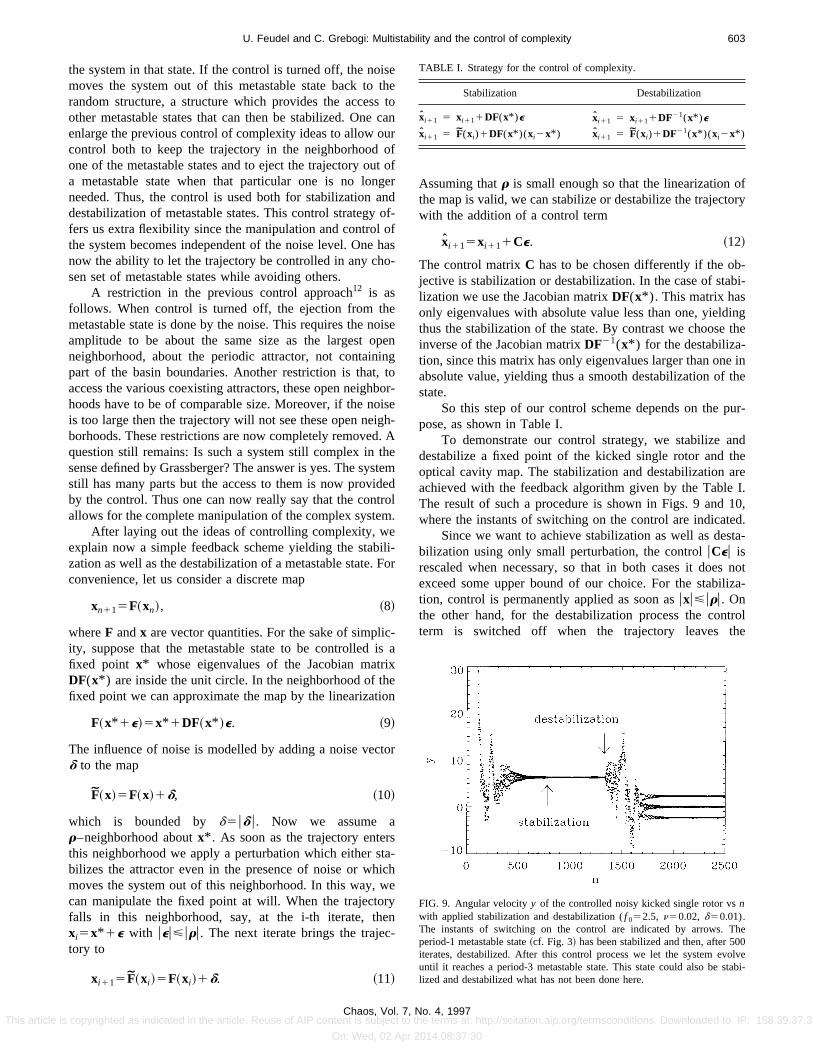
So this step of our control scheme depends on the ppose, as shown in Table I.

To demonstrate our control strategy, we stabilize adestabilize a fixed point of the kicked single rotor and toptical cavity map. The stabilization and destabilization aachieved with the feedback algorithm given by the TableThe result of such a procedure is shown in Figs. 9 andwhere the instants of switching on the control are indicat

Since we want to achieve stabilization as well as desbilization using only small perturbation, the controluCeu isrescaled when necessary, so that in both cases it doesexceed some upper bound of our choice. For the stabiltion, control is permanently applied as soon asuxu<uru. Onthe other hand, for the destabilization process the conterm is switched off when the trajectory leaves t

TABLE I. Strategy for the control of complexity.

Stabilization Destabilization

xi 11 5 xi 111DF(x* )e xi 11 5 xi 111DF21(x* )e

xi 11 5 F(xi)1DF(x* )(xi2x* ) xi 11 5 F(xi)1DF21(x* )(xi2x* )

FIG. 9. Angular velocityy of the controlled noisy kicked single rotor vsnwith applied stabilization and destabilization (f 052.5, n50.02, d50.01).The instants of switching on the control are indicated by arrows. Tperiod-1 metastable state~cf. Fig. 3! has been stabilized and then, after 50iterates, destabilized. After this control process we let the system evuntil it reaches a period-3 metastable state. This state could also be slized and destabilized what has not been done here.

No. 4, 1997the terms at: http://scitation.aip.org/termsconditions. Downloaded to IP: 158.39.37.3

2014 08:37:30

,te

duok.

of

nton

balebeno

ss

fm

rgyDi-on

L.

. B

tals

ev.

D.ev.

n

h

ws

t t

n

604 U. Feudel and C. Grebogi: Multistability and the control of complexity

This article i

r-neighborhood, i.e.,uxu.uru. To avoid specific attractorsdestabilization is switched on as soon as the trajectory entheir respective neighborhoods.

V. CONCLUSIONS

Other control schemes, besides the one presenteTable I could be chosen in different practical situations. Opurpose in using the one in Table I was to show, as a prof principle, that our ideas on controlling complexity worWe could argue that the outcome of the two experiments1,31

exhibit the kind of behavior being argued in this controlcomplexity. In the brain control experiment,1 apparentlywhen the brain is caught in an epileptic state, its neuroactivity is rather ordered, like a noisy limit cycle. In orderremove it from this state and to restore its normal functioing, the authors of Ref. 1 apply small destabilizing perturtions. Such destabilization is necessary if the ordered epitic state is attracting. If the epileptic state wouldassociated with an unstable periodic orbit embedded ochaotic attractor, as it is typical in the standard controlchaos processes, no external perturbation would be neceto restore its random chaotic activity.

ACKNOWLEDGMENTS

U. F. thanks the Deutsche Forschungsgemeinschaftsupport. This work was also supported by the A. v. Hu

FIG. 10. They variable of the controlled noisy optical cavity map witapplied stabilization and destabilization (I 50.25,n50.01,k50.4, p53.5,d50.01). The instants of switching on the control are indicated by arroThe period-1 metastable state~cf. the middle of Fig. 4! has been stabilizedand then, after 500 iterates, destabilized. After this control process we lesystem evolve until it reaches a period-1 metastable state~outside the frameof Fig. 4!. This state could also be stabilized and destabilized which hasbeen done here.

Chaos, Vol. 7,s copyrighted as indicated in the article. Reuse of AIP content is subject to

On: Wed, 02 Apr

rs

inrof

al

--p-

afary

or-

boldt Foundation and by the U.S. Department of Ene~Mathematical, Information and Computational Sciencesvision, High Performance Computing and CommunicatiProgram!.

1S. Schiff, K. Jerger, D. H. Duong, T. Chang, M. L. Spano, and W.Ditto, Nature370, 615 ~1994!.

2J. Foss, A. Longtin, B. Mensour, and J. Milton, Phys. Rev. Lett.76, 708~1996!.

3P. Marmillot, M. Kaufman, and J.-F. Hervagault, J. Chem. Phys.95, 1206~1991!.

4J. P. Laplante and T. Erneux, Physica A188, 89 ~1992!.5K. L. C. Hunt, J. Kottalam, M. D. Hatlee, and J. Ross, J. Chem. Phys.96,7019 ~1992!.

6S. M. Hammel, C. K. R. T. Jones, and J. V. Moloney, J. Opt. Soc. Am2, 552 ~1985!.

7M. Brambilla, L. A. Lugiato, and V. Penna, Phys. Rev. A43, 5114~1991!.8F. Prengel, A. Wacker, and E. Scho¨ll, Phys. Rev. B50, 1705~1994!.9U. Feudel, C. Grebogi, B. R. Hunt, and J. A. Yorke, Phys. Rev. E54, 71~1996!.

10U. Feudel, L. Poon, C. Grebogi, and J. A. Yorke, Chaos, Solitons Frac~in press!.

11C. Grebogi, H. Nusse, E. Ott, and J. A. Yorke, inDynamical Systems,Lecture Notes in Mathematics, edited by J. C. Alexander~Springer-Verlag, New York, 1988!, Vol. 1342, pp. 220–250.

12L. Poon and C. Grebogi, Phys. Rev. Lett.75, 4023~1995!.13K. Ikeda, K. Matsumoto, and K. Ohtsuka, Prog. Theor. Phys. Suppl.99,

295 ~1989!.14K. Kaneko, Physica D41, 137 ~1990!.15P. Berge´ and M. Dubois, Phys. Lett. A93, 365 ~1983!.16F. T. Arecchi, G. Giamcomelli, P. Ramazza, and S. Residori, Phys. R

Lett. 65, 2531~1990!.17K. Otsuka, Phys. Rev. Lett.65, 329 ~1990!.18C. S. Daw, C. E. A. Finney, M. Vasudevan, N. A. v. Goor, K. Nguyen,

D. Bruns, E. J. Kostelich, C. Grebogi, E. Ott, and J. A. Yorke, Phys. RLett. 75, 2308~1995!.

19E. Ott, C. Grebogi, and J. A. Yorke, Phys. Rev. Lett.64, 1196~1990!.20A. J. Lichtenberg and M. A. Lieberman,Regular and Chaotic Dynamics

~Springer, New York, 1992!.21G. Schmidt and B. W. Wang, Phys. Rev. A32, 2994~1985!.22C. Grebogi, S. McDonald, E. Ott, and J. A. Yorke, Phys. Lett. A99, 415

~1983!.23J. A. Gallas, C. Grebogi, and J. A. Yorke, Phys. Rev. Lett.71, 1359

~1993!.24H. B. Stewart, Y. Ueda, C. Grebogi, and J. A. Yorke, Phys. Rev. Lett.75,

2478 ~1995!.25Measures of Complexity, edited by L. Peliti and A. Vulpiani~Springer-

Verlag, Berlin, 1988!.26J. P. Crutchfield and K. Young, Phys. Rev. Lett.63, 105 ~1989!.27R. Badii, inChaotic Dynamics: Theory and Practice, edited by T. Bountis

~Plenum, New York, 1992!, p. 1.28J. Horgan, Sci. Am.272, 104 ~1995!.29R. Badii and A. Politi,Complexity: Hierachical Structure and Scaling i

Physics~Cambridge University Press, Cambridge, 1997!.30P. Grassberger, inFifth Mexican School on Statistical Mechanics, edited

by F. Ramos-Go´mez ~World Scientific, Singapore, 1991!, p. 57.31C. S. Daw, C. E. A. Finney, and M. Vasudevan, inThird Experimental

Chaos Conference, edited by R. Harrison, W.-P. Lu, W. L. Ditto, L.Pecora, M. Spano, and S. Vohra~World Scientific, Singapore, 1996!.

.

he

ot

No. 4, 1997the terms at: http://scitation.aip.org/termsconditions. Downloaded to IP: 158.39.37.3

2014 08:37:30