Multiscale analysis of fluxes at the turbulent/non ... · Analysis of fluxes across the...
26
PHYSICS OF FLUIDS 26, 015105 (2014) Multiscale analysis of fluxes at the turbulent/non-turbulent interface in high Reynolds number boundary layers Jimmy Philip, Charles Meneveau, a) Charitha M. de Silva, and Ivan Marusic Department of Mechanical Engineering, University of Melbourne, VIC 3010, Australia Analysis of fluxes across the turbulent/non-turbulent interface (TNTI) of turbulent boundary layers is performed using data from two-dimensional particle image ve- locimetry (PIV) obtained at high Reynolds numbers. The interface is identified with an iso-surface of kinetic energy, and the rate of change of total kinetic energy (K) inside a control volume with the TNTI as a bounding surface is investigated. Features of the growth of the turbulent region into the non-turbulent region by molecular diffu- sion of K, viscous nibbling, are examined in detail, focussing on correlations between interface orientation, viscous stress tensor elements, and local fluid velocity. At the level of the ensemble (Reynolds) averaged Navier-Stokes equations (RANS), the to- tal kinetic energy K is shown to evolve predominantly due to the turbulent advective fluxes occurring through an average surface which differs considerably from the local, corrugated, sharp interface. The analysis is generalized to a hierarchy of length-scales by spatial filtering of the data as used commonly in Large-Eddy-Simulation (LES) analysis. For the same overall entrainment rate of total kinetic energy, the theoretical analysis shows that the sum of resolved viscous and subgrid-scale advective flux must be independent of scale. Within the experimental limitations of the PIV data, the results agree with these trends, namely that as the filter scale increases, the viscous resolved fluxes decrease while the subgrid-scale advective fluxes increase and tend towards the RANS values at large filter sizes. However, a definitive conclusion can only be made with fully resolved three-dimensional data, over and beyond the large dynamic spatial range presented here. The qualitative trends from the measurement results provide evidence that large-scale transport due to the energy-containing ed- dies determines the overall rate of entrainment, while viscous effects at the smallest scales provide the physical mechanism ultimately responsible for entrainment. Data spanning over a decade in Reynolds number suggest that the fluxes (or the entrain- ment velocity) scale with the friction velocity (or equivalently the local turbulent fluctuating velocity), whereas Taylor microscale and boundary-layer thickness are the appropriate length scales at small and large filter sizes, respectively. C 2014 AIP Publishing LLC.[http://dx.doi.org/10.1063/1.4861066] I. INTRODUCTION Physical processes occurring at the sharp and corrugated surface separating turbulent from non- turbulent regions in shear flows such as jets and boundary layers have elicited considerable interest for over half a century. 1–6 Such surfaces are subjected to spatially varying advection and deformation by turbulent eddies at various scales that tend to increase the surface area. Conversely, molecular processes that typically occur at small diffusive scales in the immediate vicinity of the surface tend to smooth, and thus reduce, the surface area. Work in the 1980s and 1990s had focussed on a possibly fractal structure of surfaces in turbulence (cloud boundaries, flames, interfaces) as a reflection of deformations caused by a hierarchy of eddy sizes in the turbulent (Kolmogorov’s) inertial range. 7–11 a) Permanent address: Department of Mechanical Engineering and Center for Environmental and Applied Fluid Mechanics, The Johns Hopkins University, 3400 N. Charles Street, Baltimore, MD 21218, USA. 26, 015105-1
Transcript of Multiscale analysis of fluxes at the turbulent/non ... · Analysis of fluxes across the...
PHYSICS OF FLUIDS 26, 015105 (2014)
Multiscale analysis of fluxes at the turbulent/non-turbulentinterface in high Reynolds number boundary layers
Jimmy Philip, Charles Meneveau,a) Charitha M. de Silva, and Ivan MarusicDepartment of Mechanical Engineering, University of Melbourne, VIC 3010, Australia
(Received 26 September 2013; accepted 17 December 2013;published online 13 January 2014)
Analysis of fluxes across the turbulent/non-turbulent interface (TNTI) of turbulentboundary layers is performed using data from two-dimensional particle image ve-locimetry (PIV) obtained at high Reynolds numbers. The interface is identified withan iso-surface of kinetic energy, and the rate of change of total kinetic energy (K)inside a control volume with the TNTI as a bounding surface is investigated. Featuresof the growth of the turbulent region into the non-turbulent region by molecular diffu-sion of K, viscous nibbling, are examined in detail, focussing on correlations betweeninterface orientation, viscous stress tensor elements, and local fluid velocity. At thelevel of the ensemble (Reynolds) averaged Navier-Stokes equations (RANS), the to-tal kinetic energy K is shown to evolve predominantly due to the turbulent advectivefluxes occurring through an average surface which differs considerably from the local,corrugated, sharp interface. The analysis is generalized to a hierarchy of length-scalesby spatial filtering of the data as used commonly in Large-Eddy-Simulation (LES)analysis. For the same overall entrainment rate of total kinetic energy, the theoreticalanalysis shows that the sum of resolved viscous and subgrid-scale advective fluxmust be independent of scale. Within the experimental limitations of the PIV data,the results agree with these trends, namely that as the filter scale increases, the viscousresolved fluxes decrease while the subgrid-scale advective fluxes increase and tendtowards the RANS values at large filter sizes. However, a definitive conclusion canonly be made with fully resolved three-dimensional data, over and beyond the largedynamic spatial range presented here. The qualitative trends from the measurementresults provide evidence that large-scale transport due to the energy-containing ed-dies determines the overall rate of entrainment, while viscous effects at the smallestscales provide the physical mechanism ultimately responsible for entrainment. Dataspanning over a decade in Reynolds number suggest that the fluxes (or the entrain-ment velocity) scale with the friction velocity (or equivalently the local turbulentfluctuating velocity), whereas Taylor microscale and boundary-layer thickness arethe appropriate length scales at small and large filter sizes, respectively. C© 2014 AIPPublishing LLC. [http://dx.doi.org/10.1063/1.4861066]
I. INTRODUCTION
Physical processes occurring at the sharp and corrugated surface separating turbulent from non-turbulent regions in shear flows such as jets and boundary layers have elicited considerable interestfor over half a century.1–6 Such surfaces are subjected to spatially varying advection and deformationby turbulent eddies at various scales that tend to increase the surface area. Conversely, molecularprocesses that typically occur at small diffusive scales in the immediate vicinity of the surface tend tosmooth, and thus reduce, the surface area. Work in the 1980s and 1990s had focussed on a possiblyfractal structure of surfaces in turbulence (cloud boundaries, flames, interfaces) as a reflection ofdeformations caused by a hierarchy of eddy sizes in the turbulent (Kolmogorov’s) inertial range.7–11
a)Permanent address: Department of Mechanical Engineering and Center for Environmental and Applied Fluid Mechanics,The Johns Hopkins University, 3400 N. Charles Street, Baltimore, MD 21218, USA.
1070-6631/2014/26(1)/015105/26/$30.00 C©2014 AIP Publishing LLC26, 015105-1
015105-2 Philip et al. Phys. Fluids 26, 015105 (2014)
More recently, there has been growing interest in the structure of turbulence and transportin the vicinity of the turbulent/non-turbulent interface (TNTI hereafter).6, 12–14 The recent workhas focussed mostly on turbulent jets at moderate Reynolds numbers, specifically on the questionof whether the entrainment of the turbulent region into the non-turbulent region is dominated bylarge-scale processes through the energy-containing eddies (engulfment), or whether it is due tosmall-scale diffusive processes occurring at the interface (viscous nibbling). Recent papers6, 13, 15, 16
provide evidence supporting both views. (As an aside, we note that the term “engulfment” is typicallydefined in qualitative terms in the literature. If engulfment is used in the sense of ingestion of non-turbulent fluid by the surrounding turbulent fluid,17 then it has been observed that the contributionto total entrainment by the mass associated with the “ingestion” of fluid is small.6, 12 In such adefinition, it is difficult to separate particular length-scales responsible for the phenomena and yet,relating large and small scales to engulfment and nibbling, respectively, is not uncommon.13, 18 Herewe propose to associate the concept of “engulfment” to any non-viscous transport mechanism thatcan be associated to the large-scale energy containing eddies.16 Then a precise definition can beproposed.) The question of engulfment versus nibbling has thus far not been settled, but as mentionedby Mathew and Basu,12 if the interface has fractal scaling (outlined by Sreenivasan, Ramshankar,and Meneveau10 and Meneveau and Sreenivasan11), the two views can be reconciled: the engulfmentcaused by inertial flow structures at large and intermediate sizes increases the surface area wherediffusive processes can then act more effectively over larger areas but at the small scales. A recentanalysis by de Silva et al.19 has provided further evidence of fractal scaling of the TNTI using highReynolds number boundary layer data sets. However, a purely geometric analysis of surface area is,by itself, insufficient to answer questions directly related to physical fluxes and rates of entrainment.
The aim of the present work is to examine transport processes along the TNTI at various scales,to further clarify what physical mechanisms are responsible at each scale and to shed new light uponthe long-standing questions about large-scale engulfment versus small-scale viscous nibbling. Weshall consider the growth of the turbulent region via the fluxes of kinetic energy across the TNTI.The fluxes separate into two categories: the viscous flux (at small scales) which we associate with“nibbling”, and the advective flux (at large scales) to be associated with “engulfment”. Taking ourcue from the fractal description of the interface, we intend to ascertain/understand the scenario thatat the smallest scales only viscous flux is present, whereas at the largest scales only advective flux ispresent, while at in-between scales both operate; however, irrespective of the scale the total flux is thesame. Furthermore, we aim to examine the physical processes by which the viscous and advectivefluxes transfer kinetic energy across the interface, and how they change, if at all, with length scale.
In order to enable a clear separation of scales, flows at very high Reynolds numbers areideally required, with at least a factor δ/η ∼ 103 available (where δ is a large-scale such as theboundary layer thickness and η a small scale such as the Kolmogorov scale), in order to accountfor a factor 10 on each side of the largest and smallest scales. Also the turbulent velocity fieldneeds to be measured with sufficient accuracy to apply criteria that can discern the TNTI basedon dynamically relevant variables instead of relying only on properties of surrogate, non-dynamicfields such as passive scalars. The flow has to be probed in more than one dimension, ideally in threedimensions, but planar cuts rather than point-wise measurements can already provide meaningfulresults. Furthermore, for statistical convergence one requires large amounts of data acquired underwell-controlled experimental conditions. Over the past decade, significant progress has been madein experimental techniques such as high-resolution Particle Image Velocimetry (PIV). For example,planar PIV data by Westerweel et al.,13 Westerweel et al.,6 and Khashehchi et al.20 have been usedto study the conditional statistics at the TNTI in axisymmetric jets at moderate Re = 2000 to 6500(based on the jet diameter and nozzle velocity). They have found, as first hypothesised by Corrsinand Kistler1 (also see Ref. 21) that there exists a “jump” in the velocity tangential to the TNTI, whichis related to the jump in the Reynolds stress gradient. In fact, such a jump was also found by Chenand Blackwelder22 from the conditional profiles using hot-wires, even though it was called a “shearlayer”. Furthermore, Westerweel et al.6 have used Re = 2000 jets to measure viscous vorticity fluxesnear the TNTI for understanding the nibbling mechanism. Direct Numerical Simulations (DNSs)by da Silva, dos Reis, and Pereira18 and da Silva and Pereira23 (of planar jets) have confirmedmany of the conclusions regarding conditional averages and have also found that the size of the
015105-3 Philip et al. Phys. Fluids 26, 015105 (2014)
jump- or shear-layer thickness is related to the vortices residing on the TNTI. For boundary layers too,Semin et al.24 (at Reτ = 600) and Chauhan et al.25 (at Reτ = 14500) have found that the conditionalprofiles satisfy Reynolds’ jump conditions.21
To elucidate the role of large- and small-scale mechanisms of entrainment, Philip and Marusic16
pointed out that it is informative to separate the mean shear flows (such as jets, wakes, and boundarylayers) from the shear-free flows. Experiments and DNS of an “oscillating-grid” (shear-free flow)by Holzner et al.15, 26 have identified the importance of viscous forces originating in strain forentrainment, and that the smallest scales are of the order of Kolmogorov length scale (e.g., daSilva and Taveira27). However, the results of Holzner and Luthi28 show that the interface spreadingvelocity is not well correlated with the Kolmogorov velocity, even though they note that the viscousprocess involves a large surface area so that the global rate of turbulence spreading is set by thelargest scales of motion, in agreement with the notion of a multiscale process.10, 11 It is evident thatthe structure of turbulence and transport in the vicinity of the TNTI is associated with a range ofscales. The present investigation aims to introduce and apply an analysis approach that is specificallyaimed at identifying fluxes and transport at the TNTI at various scales, ranging between the largestto the smallest scales.
The paper is arranged as follows: Sec. II describes the experimental setup for the turbulentboundary layer experiments as well as the method for the detection of the TNTI from the veloc-ity fields; Sec. III develops relevant theoretical background to describe the evolution of the totalkinetic energy at the smallest scales governed by viscous fluxes—the nibbling process; Sec. IVintroduces a multiscale formulation characterizing the fluxes across the interface (at largest scales:purely advective fluxes—to be associated with as explained later the engulfment process, and bothnibbling and engulfment at in-between scales identified through a spatial filtering process); Sec. Vundertakes calculation and discussion of fluxes and the physical process at multiple scales based onthe experimental data; and Sec. VI summaries and draws final conclusions. Throughout the paper,x, y, and z represent the streamwise, spanwise, and wallnormal directions, and u, v, and w (or u1, u2,and u3), the corresponding velocities. Whenever physical quantities are normalised by the viscouslength and velocity scales ν/uτ and uτ , respectively, they are represented by plus, + symbols, e.g.,normalised length �+ = �/(ν/uτ ), velocity u+ = u/uτ , etc.
II. EXPERIMENTAL SETUP AND INTERFACE DETECTION
In this work, we apply planar PIV measurements in the wall-normal/streamwise direction to aflow for the purpose of investigating the interface characteristics at significantly higher Reynoldsnumbers than prior works.6, 24 We examine physical transport processes across the TNTI using twoexperimental data sets in very high Reynolds number boundary layers, at Reδ = U∞δ/ν ≈ 2.37 × 10⁵,and 4.6 × 10⁵, corresponding to turbulent Reynolds numbers based on friction velocity Reτ = uτ δ/ν≈ 7870 and 14500. The Taylor Reynolds number at the mean interface location25 estimated usingisotropic relations and hot-wire data are ReλT = λT u′/ν ≈ 230 and 300. Some relevant parametersfor the two databases are provided in Table I. Note that Table I also includes a smaller databaseof Adrian, Meinhart, and Tomkins29 at Reτ = 2790 (ReλT = 125 at the mean interface location)available in the public domain, which shall be used only in reference to Figure 11 to understand the
TABLE I. Experimental parameters for the PIV databases, where Reδ = δU∞/ν, Reθ = θU∞/ν, and θ is the momentumthickness.
U∞ uτ δ
Reτ Reδ Reθ [ms−1] [ms−1] [m] �x+ × �z+ No. of images
2790a 0.7 × 10⁵ 6845 11.4 0.4 0.1 36 × 25 507870 2.4 × 10⁵ 22400 10.1 0.33 0.36 52 × 52 100014500 4.6 × 10⁵ 40800 20.0 0.63 0.35 49 × 49 1250
aThe dataset at Reτ = 2790 is from Adrian, Meinhart, and Tomkins29 and is available in the public domain.
015105-4 Philip et al. Phys. Fluids 26, 015105 (2014)
Flow
0.8m
0.5m
Field of view located 21m from trip
Bottom cameras with higher magnification
Top cameras with lower magnification
z
x
y
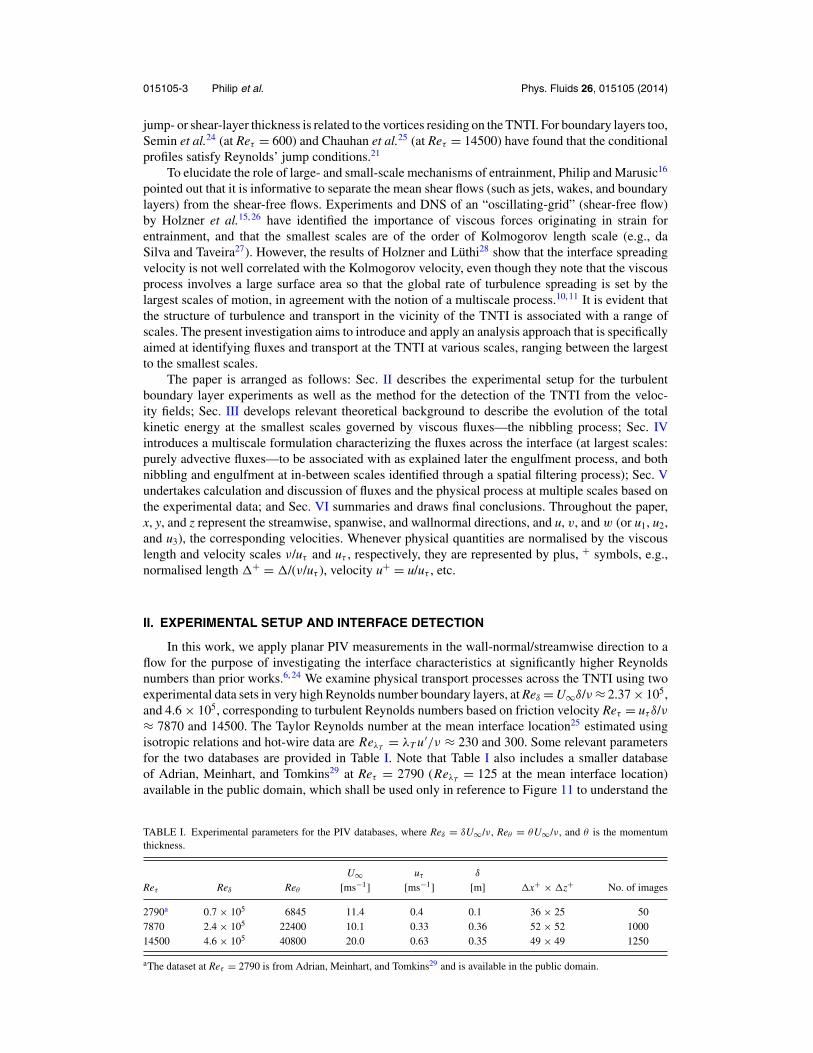
FIG. 1. Experimental setup for the planar PIV measurements using eight cameras in the High Reynolds Number BoundaryLayer Wind Tunnel at the University of Melbourne.
Re-scaling. We note that for the different boundary layer databases, the PIV interrogation windowsize is about 4 to 6 times the Kolmogorov length scale in the outer region.
Figure 1 shows the experimental setup for the PIV measurements performed in the HighReynolds Number Boundary Layer Wind Tunnel (HRNBLWT) at the University of Melbourne’sWalter Bassett Aerodynamics Laboratory. The region of interest is illuminated by a laser sheetin the spanwise centre of the tunnel, beamed from below the glass floor employing a SpectraPhysics “QuantaRay” Nd:YAG laser rated 400 mJ per pulse at 532 nm. PIV images are obtainedsimultaneously on eight PCO 4000 cameras (4008×2672 pixels), four cameras arranged above therest, with the bottom cameras having a higher magnification and covering a smaller area, and anoverlap of about 2 cm between images. The eight individual vector fields are later stitched to providea single 2D velocity field. This provides a large dynamic range which is particularly suited to thepresent study where we are interested in fluxes at the smallest scales to the largest ones. Furtherdetails of the experiments (along with the comparisons of mean and turbulent statistics to hot-wiredata) and processing of PIV images can be found in Chauhan et al.25 and de Silva et al.30
Traditionally, the interface has been detected based on hot-wire velocity signals (e.g., seeRef. 31 for a comprehensive list of detector functions commonly used at that time), wherein it is nottoo difficult to distinguish the relatively quiet regions from those with high fluctuations. Techniquesemploying scalars (ideally with relatively high Schmidt number) are also popular for interfacedetection, both using 1D data (or a rake) from resistance thermometers (employing temperature inthe turbulent region as a marker22) and 2D imaging of passive dyes in experiments6, 10, 32–34 as well asin Direct Numerical Simulations.35 More recently a threshold on vorticity magnitude has been usednot only to distinguish turbulent from the non-turbulent regions12, 36–38 primarily in DNS databasesbut also in moderately low Reynolds number turbulent boundary layer experiments24 where theyhad 3D velocity information from Tomographic-PIV measurements.
It is known (starting from the work of Corrsin and Kistler1) that velocity in the non-turbulentregion differs from that in the turbulent region, and thus mean velocity1, 39 or variance of velocityfluctuations40 have also been used for interface detection. Of the plethora of techniques availablenot all are suited for every type of measurement. In the present case, we have no passive scalar andvelocity fields that are obtained from PIV (which are generally at a lower resolution than hot-wiresand more prone to noise, especially in the non-turbulent region of the boundary layer due to largevelocities there, unlike jets). Vorticity based criteria tend to include nearly irrotational islands withina fully turbulent region, which in turn leads to a highly intermittent and unconnected interface thatmay also be affected by the inherent “inner intermittency” within the turbulent region. Consequently,in this work we employ the kinetic energy of the flow for interface detection. In order to associate thenon-turbulent outer region with zero kinetic energy, we use the kinetic energy in the frame moving
015105-5 Philip et al. Phys. Fluids 26, 015105 (2014)
0 0.25 0.5 0.75 1 1.25 1.5 1.75 20
0.25
0.5
0.75
1
z/δ
x/δ
non-turbulent
turbulent
(a)
0.36 0.38 0.4 0.42 0.44 0.46
0.7
0.72
0.74
z/δ
x/δ
(b)
0.36 0.38 0.4 0.42 0.44 0.46
0.7
0.72
0.74
z/δ
x/δ
(c)log10[2K/U2∞]
−3.5
−3
−2.5
−2
−1.5
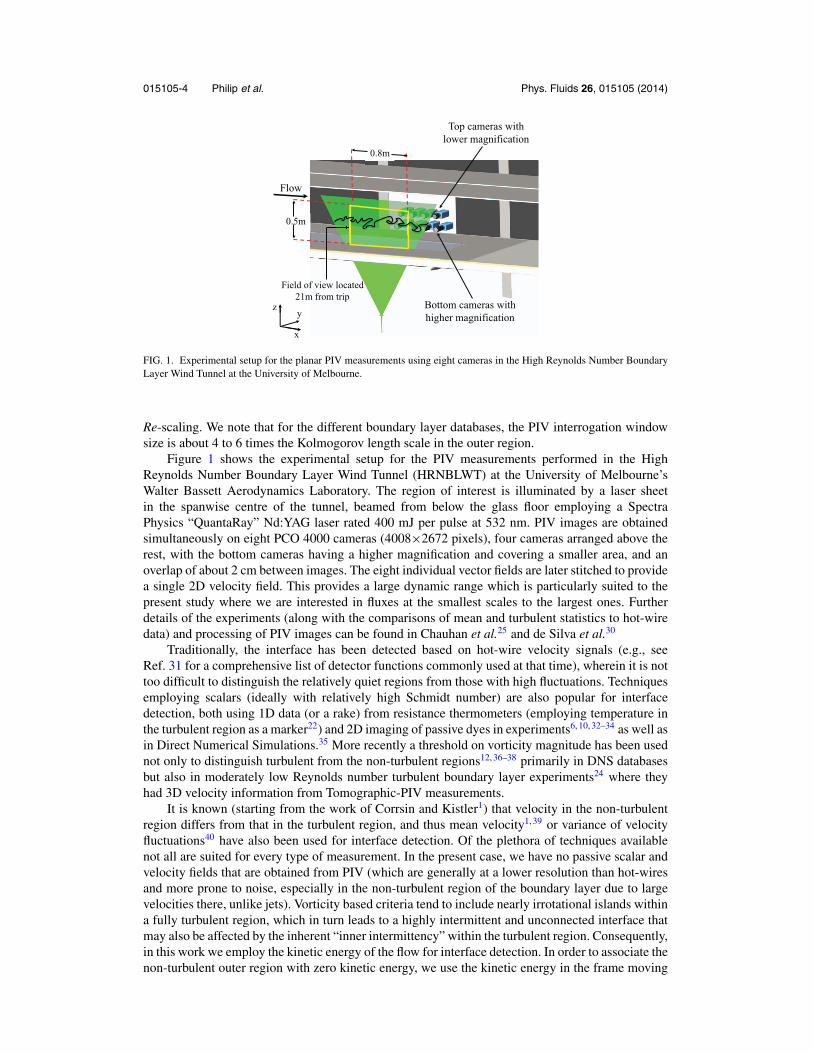
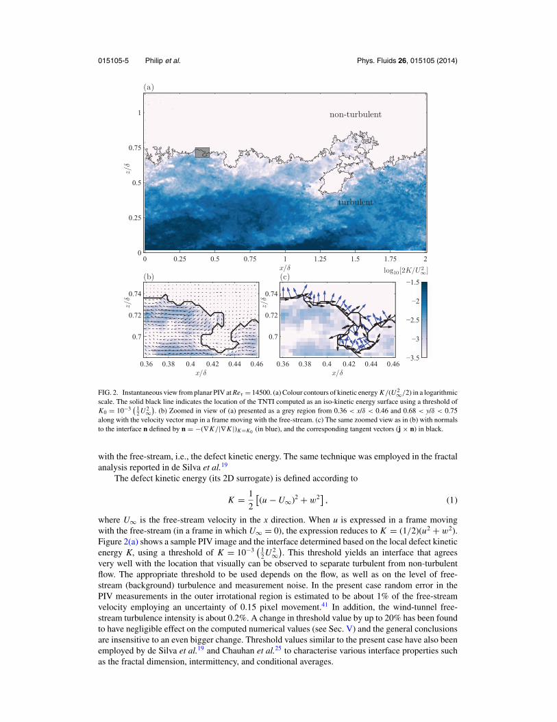
FIG. 2. Instantaneous view from planar PIV at Reτ = 14500. (a) Colour contours of kinetic energy K/(U 2∞/2) in a logarithmicscale. The solid black line indicates the location of the TNTI computed as an iso-kinetic energy surface using a threshold ofK0 = 10−3
( 12 U 2∞
). (b) Zoomed in view of (a) presented as a grey region from 0.36 < x/δ < 0.46 and 0.68 < y/δ < 0.75
along with the velocity vector map in a frame moving with the free-stream. (c) The same zoomed view as in (b) with normalsto the interface n defined by n = −(∇K/|∇K |)K=K0 (in blue), and the corresponding tangent vectors (j × n) in black.
with the free-stream, i.e., the defect kinetic energy. The same technique was employed in the fractalanalysis reported in de Silva et al.19
The defect kinetic energy (its 2D surrogate) is defined according to
K = 1
2
[(u − U∞)2 + w2] , (1)
where U∞ is the free-stream velocity in the x direction. When u is expressed in a frame movingwith the free-stream (in a frame in which U∞ = 0), the expression reduces to K = (1/2)(u2 + w2).Figure 2(a) shows a sample PIV image and the interface determined based on the local defect kineticenergy K, using a threshold of K = 10−3
(12U 2
∞). This threshold yields an interface that agrees
very well with the location that visually can be observed to separate turbulent from non-turbulentflow. The appropriate threshold to be used depends on the flow, as well as on the level of free-stream (background) turbulence and measurement noise. In the present case random error in thePIV measurements in the outer irrotational region is estimated to be about 1% of the free-streamvelocity employing an uncertainty of 0.15 pixel movement.41 In addition, the wind-tunnel free-stream turbulence intensity is about 0.2%. A change in threshold value by up to 20% has been foundto have negligible effect on the computed numerical values (see Sec. V) and the general conclusionsare insensitive to an even bigger change. Threshold values similar to the present case have also beenemployed by de Silva et al.19 and Chauhan et al.25 to characterise various interface properties suchas the fractal dimension, intermittency, and conditional averages.
015105-6 Philip et al. Phys. Fluids 26, 015105 (2014)
Figures 2(b) and 2(c) show a zoomed in view of a portion of the interface (as indicated by thegrey region in Figure 2(a)) along with velocity vectors, and local normals (n = −∇K/|∇K |K=K0 ,where K0 is the threshold level) and tangents to the interface defined as t = j × n, where j is theunit vector in the y-direction perpendicular to the measurement plane. Notice that, in general, (aswell as in Figure 2(a)) one can also observe patches of non-turbulent regions inside the turbulentregion. With the present PIV measurements, we cannot ascertain if these patches are connected tothe outside non-turbulent region three-dimensionally or if they are genuinely disconnected volumesof non-turbulent regions. In any case, we shall not include these patches in the analysis whenperforming averages over the interface, and we will consider TNTI as the longest boundary thatseparates the main turbulent region from the outside non-turbulent region. Finally, we remark that(albeit for jets) based on DNS and experimental data there is evidence that using different interfacedetection criteria do not significantly change the interface characteristics.39
III. KINETIC ENERGY EQUATION: FLUXES AT THE SMALLEST SCALES
Having observed that kinetic energy relative to the free stream provides a meaningful criterionto determine the TNTI, we now turn to the dynamics and transport processes associated with kineticenergy. We consider the transport of defect kinetic energy K(x, t), defined according to
K (x, t) = 1
2[u(x, t) − U]2, (2)
where U is the constant velocity in the free-stream far outside the boundary layer. That is, in atraditional frame of reference attached to the wall and a free-stream moving in the positive direction(x-direction with unit vector i), we have U = U∞i (= U1i depending on the context), while in aframe moving with the free-stream velocity in which the wall moves, we have U = 0. Note thatK(x, t) includes the kinetic energy in both the mean flow defect velocity field, as well as all thekinetic energy in the turbulence since no averaging has yet been performed.
The momentum equation for a Newtonian incompressible flow (with viscous stress tensorτ ν
i j = 2νSi j , where Sij is the strain-rate tensor), written for the momentum defect with respect to aconstant free stream velocity U, is
∂
∂t(ui − Ui ) + u j
∂
∂x j(ui − Ui ) = − 1
ρ
∂p
∂xi+ ∂τ ν
i j
∂x j. (3)
Multiplying by the velocity defect, ui − Ui, results in the equation for K(x, t):
∂K
∂t+ ∂
∂xi(ui K ) = ∂
∂xi
(−(u j − U j )
p
ρδi j + (u j − U j )τ
νj i
)− τ ν
i j
∂u j
∂xi. (4)
Now consider a boundary layer control volume (Vbl) including as its top surface the TNTI assketched in Figure 3(a). The interface is defined as a K = K0 iso-surface, and the dashed line isinstantaneously coincident with the interface (fixed, not moving with the interface). For a boundarylayer, we have used K0 = c0
12U 2
∞ and we specify the (small) dimensionless factor c0, e.g., c0 =10−3 as was used in de Silva et al.19 and Figure 2. The kinetic energy equation for the total kineticenergy in the boundary layer KVbl = ∫
VblK d3x in the (fixed) control volume reads
dKVbl
dt= −
∫∫Sbl
[ui K − 2νSi j (u j − U j )
]ni d S −
∫∫Sbl
(p
ρ
)(ui − Ui )ni d S −
∫∫∫Vbl
εdV, (5)
where ε = τ νi j∂u j/∂xi is the viscous dissipation rate. The advective flux can be further decomposed,
and the kinetic energy equation is rewritten as follows:
dKVbl
dt= −
∫∫Sbl
KUi ni d S −∫∫
Sbl
(K + p
ρ
)(ui − Ui )ni d S
−(
−2ν
∫∫Sbl
Si j (u j − U j )ni d S
)−
∫∫∫Vbl
εdV . (6)
015105-7 Philip et al. Phys. Fluids 26, 015105 (2014)
(a)
(b)
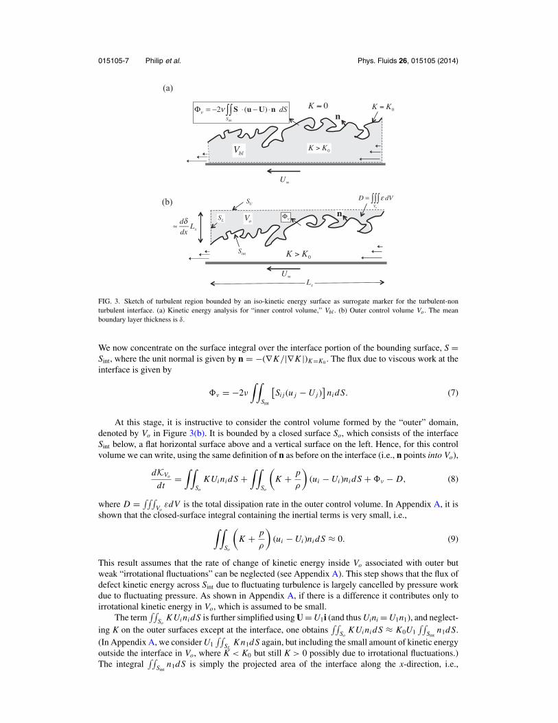
FIG. 3. Sketch of turbulent region bounded by an iso-kinetic energy surface as surrogate marker for the turbulent-nonturbulent interface. (a) Kinetic energy analysis for “inner control volume,” Vbl . (b) Outer control volume Vo. The meanboundary layer thickness is δ.
We now concentrate on the surface integral over the interface portion of the bounding surface, S =Sint, where the unit normal is given by n = −(∇K/|∇K |)K=K0 . The flux due to viscous work at theinterface is given by
�ν = −2ν
∫∫Sint
[Si j (u j − U j )
]ni d S. (7)
At this stage, it is instructive to consider the control volume formed by the “outer” domain,denoted by Vo in Figure 3(b). It is bounded by a closed surface So, which consists of the interfaceSint below, a flat horizontal surface above and a vertical surface on the left. Hence, for this controlvolume we can write, using the same definition of n as before on the interface (i.e., n points into Vo),
dKVo
dt=
∫∫So
KUi ni d S +∫∫
So
(K + p
ρ
)(ui − Ui )ni d S + �ν − D, (8)
where D = ∫∫∫Vo
εdV is the total dissipation rate in the outer control volume. In Appendix A, it isshown that the closed-surface integral containing the inertial terms is very small, i.e.,∫∫
So
(K + p
ρ
)(ui − Ui )ni d S ≈ 0. (9)
This result assumes that the rate of change of kinetic energy inside Vo associated with outer butweak “irrotational fluctuations” can be neglected (see Appendix A). This step shows that the flux ofdefect kinetic energy across Sint due to fluctuating turbulence is largely cancelled by pressure workdue to fluctuating pressure. As shown in Appendix A, if there is a difference it contributes only toirrotational kinetic energy in Vo, which is assumed to be small.
The term∫∫
SoKUi ni d S is further simplified using U = U1i (and thus Uini = U1n1), and neglect-
ing K on the outer surfaces except at the interface, one obtains∫∫
SoKUi ni d S ≈ K0U1
∫∫Sint
n1d S.(In Appendix A, we consider U1
∫∫SL
K n1d S again, but including the small amount of kinetic energyoutside the interface in Vo, where K < K0 but still K > 0 possibly due to irrotational fluctuations.)The integral
∫∫Sint
n1d S is simply the projected area of the interface along the x-direction, i.e.,
015105-8 Philip et al. Phys. Fluids 26, 015105 (2014)
∫∫SI
n1d S ≈ −dδ/dx Axy where Axy is the footprint area of the control volume. The negative signarises because n points into Vo and thus n1 < 0 on average if dδ/dx > 0).
Finally, we obtain
dKVo
dt+ U1 K0
dδ
dxAxy = �ν − D. (10)
Note that the integrated quantity KVo represents kinetic energy in the full defect velocity field,including mean flow and turbulent fluctuations. In a frame moving with the free-stream velocity, U1
= 0, thus the term U1K0Axydδ/dx vanishes, and dKVo/dt is expected to be positive (increase of kineticenergy in the outer volume Vo in time). On the other hand, in a frame attached to the wall, on averagewe have 〈dKVo/dt〉 = 0 due to stationarity, but it is replaced by the term U1K0dδ/dxAxy (recall thatU1 = U∞), which represents the positive advective flux of K0 due to the free-stream velocity. In asense, this term then “counteracts” the viscous diffusion �ν “moving back defect kinetic energy”into the control volume and out of Vo along the interface. The dissipation D is expected to be smallin the outer region. Thus Eq. (10) shows that the growth rate 〈dKVo/dt〉 or U1 K0
dδdx Axy of defect
kinetic energy in the turbulent boundary layer is caused by the viscous flux at the interface, �ν .Our aim later in the paper is to examine �ν from PIV data. A two-dimensional surrogate that
can be determined from planar PIV data (in the x1-x3 plane) along the intersection of the interfacewith the measurement plane is:
�2Dν = −2ν
∫ s f
s=0
(Si j u j
)ni ds, i, j = 1, 3, (11)
involving only two components and where the integration is performed along an interface-followingcoordinate s that goes from the beginning of the interface at s = 0 to the end s = sf.
IV. MULTISCALE PROPERTIES OF FLUXES AT THE TNTI
In order to examine multiscale properties of entrainment/nibbling/fluxes at the TNTI defined interms of kinetic energy, we consider the kinetic energy field associated with descriptions at variousscales.
A. Mean flow: Ensemble (Reynolds) averaged formulation
We begin by the description at the level of Reynolds Average Navier-Stokes (RANS) andensemble averaging, i.e., emphasizing processes occurring at the level of the mean flow and thelargest scales of turbulence. At this level, surfaces are essentially flat, growing slowly like themean boundary layer. Denoting ensemble average by an over-bar, the kinetic energy in the meandefect flow is defined as K R = 1
2 (ui − Ui )2. The superscript “R” refers to Reynolds averaging (seeFigure 4(c)). The fate of kinetic energy in the mean defect flow is governed by
∂K R
∂t+ ∂
∂xi(ui K R) = − ∂
∂xi
(1
ρ(u j − U j )pδi j − (u j − U j )τ
νj i + (u j − U j )u′
i u′j
)−τ ν
j i
∂u j
∂xi+ u′
i u′j
∂u j
∂xi. (12)
However, there is also turbulent kinetic energy k R = 12 u′
i u′i (where u′
i = ui − ui ), which should beadded to KR to obtain total kinetic energy K = K R + k R that can be compared to the total kineticenergy considered in Sec. III.
The transport equation for turbulent kinetic energy k R = 12 u′
i u′i reads
∂k R
∂t+ ∂
∂xi(ui k
R) = − ∂
∂xi
(1
ρu′
j p′δi j − τ ′νj i u
′j + 1
2u′
j2u′
i
)− u′
i u′j
∂u j
∂xi− ε + τ ν
j i
∂u j
∂xi. (13)
015105-9 Philip et al. Phys. Fluids 26, 015105 (2014)
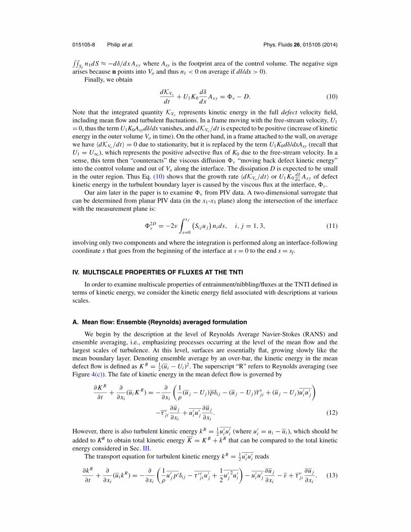
FIG. 4. Sketch of turbulent region bounded by iso-kinetic energy surface at various scales. (a) Original scale, resolvingviscous stresses, (b) filtered at intermediate scale �, (c) ensemble averaged (RANS) based on mean flow.
The transport equation for the total kinetic energy can be obtained by adding both equations,i.e.,
∂K
∂t+ ui
∂K
∂xi= − ∂
∂xi
(1
ρ
[(u j − U j )p + u′
j p′]δi j + (u j − U j )u′
i u′j + 1
2u′
j2u′
i
)− ε, (14)
where viscous fluxes have been neglected since at high Reynolds numbers away from the wall theyare expected to be small.
The interface associated with the mean flow is now defined as where the total energy K = K0,using the same threshold as in Secs. II and III. The unit vector is defined as n ≡ −(∇K/|∇K |)K=K0
,which differs from taking the average of the instantaneous ni due to nonlinearities in the definitionsof kinetic energy and the division by the absolute value of the gradient. This definition can benaturally generalized to other scales later on and has a clear physical interpretation in terms of thekinetic energy in the flow. For example, see Appendix B (Figure 12) for a comparison of differentmethods to identify the interface with the same threshold value. The threshold K0 to be employedwill be quite small and thus it will define the “outer skin” of the turbulent region. Such a surface canbe considered a “RANS-level interface” separating turbulence from non-turbulence, even thoughthe interface region is expected to be quite “thick,” on the order of the outer integral scale δ. Thus,one has to consider the “RANS-level interface” at large scales to be able to interpret it as a “sharp”interface.
Following similar steps as in Sec. III, we define inner and outer control volumes, separatedby a (smooth) interface. For the outer control volume (denoted as VRo), the total energy KVRo =∫∫∫
VRoK dV , obeys:
dKVRo
dt+ U1 K0
dδ
dxAxy =
∫∫SRo
(K + p
ρ
)(ui − Ui )ni d S + �A − DR, (15)
where,
�A =∫∫
SRint
[(u j − U j )u′
i u′j + 1
2u′
j2u′
i + 1
ρu′
i p′]
ni d S, (16)
is the flux of kinetic energy across the interface due to turbulent motions (including advection byturbulent fluctuations and pressure fluctuations), affecting the budget of kinetic energy in the mean
015105-10 Philip et al. Phys. Fluids 26, 015105 (2014)
defect flow, and
DR =∫∫∫
VRo
εdV . (17)
A “Bernoulli”-like argument, in which we assume that K + p/ρ ≈ p∞/ρ (for RANS a steadyBernoulli framework is assumed to be appropriate in the irrotational region) will lead to∫∫
SRo
(K + p
ρ
)(ui − Ui )ni d S ≈ 0. Hence,
dKVRo
dt+ U1 K0
dδ
dxAxy = �A − DR . (18)
The flux �A can be considered to be a definition of the “entrainment-rate” by the large scalessince the Reynolds stress tensor and turbulent transport is dominated by the large scales. We shallalso identify this term as corresponding to “large-scale engulfment” since it is associated with theReynolds stresses that depend mostly on the energy-containing eddies.
And, since the left-hand side of (18) is the same as that in (10) for the total energy in theinstantaneous description, and the dissipation terms are also the same, it follows that the fine-grainedand coarse-grained fluxes should be equal, i.e., �A = �ν , at least in the averaged sense.
At low Reynolds numbers, the viscous fluxes from the mean flow should be added to �A.Considering Figure 4(a), the corresponding interface is shown with the thick dashed line, assumingit to be almost linear, i.e., with an angle θbl ≈ tan −1(dδ/dx).
B. Filtered flow: LES formulation
Next, we consider turbulence at various scales, using “coarse-grained” filtered velocities asis usually applied in Large Eddy Simulations (LES). Consider the kinetic energy in turbulence atscales equal to and larger than some scale �: K � = 1
2 ui ui . The “tilde” refers to, for example, a boxfiltering, i.e., a convolution of the velocity components with a top-hat filter function G�, namelyui ≡ G� ∗ ui . This defines a kinetic energy field that is smoother than the original. The evolutionequation for K�(x, t) is obtained by starting from the filtered momentum equation,42, 43 written hereas before for the (filtered) velocity defect:
∂(ui − Ui )
∂t+ uk
∂(ui − Ui )
∂xk= − 1
ρ
∂ p
∂xi+ ∂τ ν
i j
∂x j− ∂τ�
i j
∂x j, (19)
where τ�i j = ui u j − ui u j is the “subgrid-scale” (SGS) or “subfilter-scale” stress tensor. Instanta-
neous fields of SGS stress tensor in 2D planes can be obtained from PIV data simply by box-filteringthe product uiuj (e.g., i, j = 1, 3, in vertical wall-normal planes in boundary layers) and at each pointsubtracting the product of the filtered velocities.44–46 Thus in the present case, one obtains threespatial fields for τ�
11(x, z, t0), τ�33(x, z, t0), and τ�
13(x, z, t0).Multiplying (19) by (ui − Ui ) leads to the equation for K �(x, t) = 1
2 (ui − Ui )2, the kineticenergy in the large-scale field of the velocity defect:
∂K �
∂t+ ∂
∂xi(ui K �) = − ∂
∂xi
(1
ρ(u j − U j ) pδi j − (u j − U j )τ
νi j + (u j − U j )τ
�i j
)− τ ν
i j Si j + τ�i j Si j .
(20)
There is also kinetic energy contained in the SGS motions, k� = 12 (ui ui − ui ui ), and its
transport equation is given by[∂
∂t+ u j
∂
∂x j
]k� = − ∂
∂x j
(1
ρ( pui − pui )δi j + (−uiτ
νi j + ui τ
νi j ) − uiτ
�i j +
1
2(u j ui ui − u j ui ui )
)− ˜τ ν
i j Si j + τ νi j Si j − τ�
i j Si j . (21)
015105-11 Philip et al. Phys. Fluids 26, 015105 (2014)
The total kinetic energy in the defect field, when viewed at scale � is given by K = K � + k�
and its transport equation at that scale is obtained by adding the equations for K � and k�, resultingin [
∂
∂t+ u j
∂
∂x j
](K � + k�) = − ∂
∂x j
(1
ρ( pui − Ui p)δi j − (uiτ
νi j − Ui τ
νi j )
+ (u j ui ui − u j ui ui )/2 − Uiτ�i j
)− ˜τ ν
i j Si j . (22)
We define the interface as the iso-level of K = K � + k� at K0 = c012U 2
∞ as before, andthe unit normal is denoted according to n = −(∇ K/|∇ K |)K=K0
. Notice that, (22) reduces to (4)in the limit � → 0, corresponding to the unfiltered field. In the limit of large � with � exceeding theturbulence integral scale and to the degree that spatial and ensemble averaging yield similar results(this does not hold in flows with strong spatial mean inhomogeneities), the formulation tends to thatof RANS, where (22) reduces to (14) (assuming as in (14) that the viscous stress gradient terms aresmall). Also, we recall that the notion of a “sharp interface” can be applied to the LES-level interfaceonly when viewed at scales larger than �, whereas, at scales smaller than � the interface is smearedout by construction.
We now apply the control volume argument to the total kinetic energy in the outer controlvolume bounded below by the filtered interface at scale � (see Figure 4(b) for the filtered controlvolume and Figures 4(a) and 4(c) for comparison with no filtering and RANS case). Defining,KV�o = ∫∫∫
V�oK dV and χ�
j ≡ pu j − pu j , we obtain
dKV�o
dt+ U1 K0
dδ
dxAxy =
∫∫S�o
(K + p
ρ
)(u j − U j )n j d S + �A� + �ν� − D�, (23)
where
�A� =∫∫
S�int
[1
2(u j ui ui − u j ui ui ) − Uiτ
�i j + 1
ρχ�
j
]n j d S (24)
is the flux of kinetic energy across the interface due to turbulent motions at the scale �, whereas,
�ν� = −2ν
∫∫S�int
[(˜ui Si j − Ui Si j )
]n j d S (25)
is the contribution of viscous fluxes to the kinetic energy transport across the interface, and,
D� =∫∫∫
V�o
εdV . (26)
Resorting again to the Bernoulli equation as before, wherein, (K + p/ρ) ≈ p∞/ρ is assumed, leadsto,
dKV�o
dt+ U1 K0
dδ
dxAxy = �A� + �ν� − D�. (27)
Note that in the definition of D�, the integration and the filtering commute. Hence, if the controlvolume V�o is sufficiently large, it is quite reasonable to assume that all of these total rates ofdissipation are essentially the same: D ≈ DA ≈ D�, if not exactly for instantaneous fields, at leastafter ensemble averaging. Since the left-hand side of Eqs. (10), (18) and (27) should also be thesame (neglecting fluctuations in the definitions of δ), it follows that the averaged
�ν ≈ �A ≈ �A� + �ν�, (28)
regardless of �. If only planar experimental data are available, 2D surrogates �2DA� and �2D
ν� canbe defined by restricting i, j = 1, 3. Such 2D surrogate quantities, however, will involve missinginformation from “surface folds” and components in the directions normal to the data plane especiallyat smaller scales. At larger scales, when the flow approaches the mean which is two-dimensional, the2D surrogate definitions are expected to be correct, but at small scales, where the flow structure is
015105-12 Philip et al. Phys. Fluids 26, 015105 (2014)
highly 3D, important contributions would be missing. The concept of local isotropy may be invokedat scales below some threshold, i.e., for � < �iso. However, the experimental data show that verysmall scales would be needed to approach such local isotropy (cf., Sec. V A and Appendix C). Suchinherent limitations of 2D surrogates will need to be kept in mind when interpreting measurementresults.
The above analysis is carried out for a control volume Vo(x, t = t0) that is fixed at an instant intime, t0. A similar analysis can be performed based on a deforming control volume which changeswith time, Vdo(t). The control volume Vdo is attached to the evolving interface which moves atvelocity uint. See Appendix D for the details. The approach leads to the definition of the localentrainment velocity v = u − uint (e.g., Ref. 47). At any scale �, it is shown (see Appendix D) thatthe total flux, (�A� + �ν�) can be used to define a surface averaged net entrainment velocity atthat scale, v�
s , such that, v�s S(�) = (�A� + �ν�)/K0, where S(�) is the surface area at a particular
scale �. Since the total flux at any scale has to be a constant, it implies that v�s S(�) is also a constant.
V. EXPERIMENTAL RESULTS AND DISCUSSION
Velocity fields from the PIV databases are employed to calculate the various energy fluxes acrossthe interface. Accordingly, the surface integrals over the interface are replaced by line integrals alongthe wrinkled line over the contour corresponding to the interface on the 2D vector field. Fluxes arecalculated in a reference frame moving with the free stream velocity, i.e., U = 0. Energy fluxesfor the three cases will be presented sequentially, beginning with the unfiltered case, the RANScase, and finally the filtered/LES case. Gradients are calculated using the method of least squares.41
Specifically, we employ a 2D Savitzky-Golay least square scheme with a stencil of 5 × 5 and a thirdorder polynomial fitting.
Before presenting results, we note that the data analysis to obtain viscous flux �2Dν for the
unfiltered case is expected to lead to under-predictions of the flux since the spacing between the datapoints (of ≈10η to 4η, from the mean interface location to the outer edge of the boundary layer)does not extend to scales at or below the Kolmogorov length scale (η). Therefore, the measured�2D
ν is denoted by including a hat, �2Dν , to represent the resolution effect inherent in the data. For
the same reason, experimentally measured �2Dν� is denoted by �2D
ν�. Furthermore, in the case of thesubgrid flux �2D
A� as function of filter scale �, the lack of data on the pressure field prevents us frommeasuring the subgrid pressure contribution χ�
j (although some estimates shall be provided). As aresult of these limitations, the focus of the analysis will be on the general trends of measured terms,rather than their precise numerical values.
A. Kinetic energy fluxes at small scales: Viscous effects
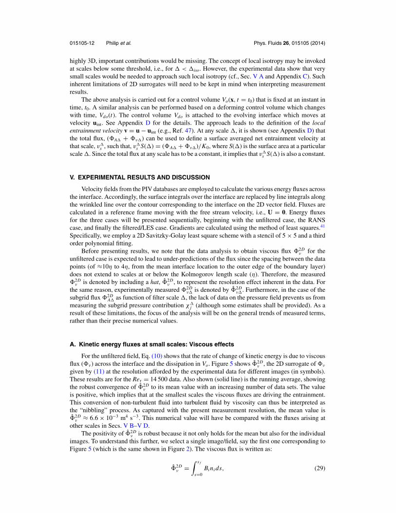
For the unfiltered field, Eq. (10) shows that the rate of change of kinetic energy is due to viscousflux (�ν) across the interface and the dissipation in Vo. Figure 5 shows �2D
ν , the 2D surrogate of �ν
given by (11) at the resolution afforded by the experimental data for different images (in symbols).These results are for the Reτ = 14 500 data. Also shown (solid line) is the running average, showingthe robust convergence of �2D
ν to its mean value with an increasing number of data sets. The valueis positive, which implies that at the smallest scales the viscous fluxes are driving the entrainment.This conversion of non-turbulent fluid into turbulent fluid by viscosity can thus be interpreted asthe “nibbling” process. As captured with the present measurement resolution, the mean value is�2D
ν ≈ 6.6 × 10⁻³ m4 s−3. This numerical value will have be compared with the fluxes arising atother scales in Secs. V B–V D.
The positivity of �2Dν is robust because it not only holds for the mean but also for the individual
images. To understand this further, we select a single image/field, say the first one corresponding toFigure 5 (which is the same shown in Figure 2). The viscous flux is written as:
�2Dν =
∫ s f
s=0Bi ni ds, (29)
015105-13 Philip et al. Phys. Fluids 26, 015105 (2014)
FIG. 5. Symbols: measured viscous flux of kinetic energy at the TNTI, �2Dν (as resolved with the present spatial accuracy),
for each of the 1250 vector fields at Reτ = 14500. The solid (red) line shows the running average of �2Dν with increasing
number of images Ni. The units of the viscous flux shown are m4s−3.
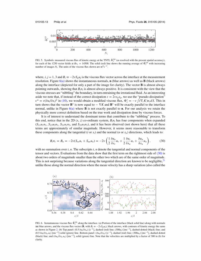
where, i, j = 1, 3 and Bi ≡ −2νSijuj is the viscous flux vector across the interface at the measurementresolution. Figure 6(a) shows the instantaneous normals, n (blue arrows) as well as B (black arrows)along the interface (depicted for only a part of the image for clarity). The vector B is almost alwayspointing outwards, showing that Bini is almost always positive. It is consistent with the view that theviscous stresses are “nibbling” the boundary, in turn entraining the irrotational fluid. As an interestingaside we note that, if instead of the correct dissipation ε = 2νsijsij, we use the “pseudo-dissipation”ε* = ν(∂ui/∂xi)2 in (10), we would obtain a modified viscous flux, �∗
ν = −ν∫
(∇i K )ni d S. This inturn shows that the vector B∗ is now equal to − ∇K and B∗ will be exactly parallel to the interfacenormal, unlike in Figure 6(a) where B is not exactly parallel to n. For our analysis we retain thephysically more correct definition based on the true work and dissipation done by viscous forces.
It is of interest to understand the dominant terms that contribute to the “nibbling” process. Tothis end, notice that in the 2D (x, z) co-ordinate system, Bini has four components when expanded(S11u1n1, S13u3n1, S31u1n3, and S33u3n3), and it has been observed (not shown here) that all theseterms are approximately of similar magnitude. However, it seems more reasonable to transformthese components along the tangential (t or xt) and the normal (n or xn) directions, which leads to:
Bi ni = Bn = −2ν(Stnut + Snnun) = −2ν
(1
2
∂un
∂xtut + 1
2
∂ut
∂xnut + ∂un
∂xnun
), (30)
with no summation over t, n. The subscripts t, n denote the tangential and normal components of thetensor and vectors. Evaluations from the data show that the first term on the rightmost side of (30) isabout two orders of magnitude smaller than the other two which are of the same order of magnitude.This is not surprising because variations along the tangential direction are known to be negligible,21
unlike those along the normal direction where the mean velocity has a sharp variation (also called the
0.36 0.38 0.4 0.42 0.440.68
0.7
0.72
0.74
z/δ
x/δ
(a)
−300
0
300
0.5∂
ut/
∂n
,ut
(b)
1.88 1.92 1.96 2 2.04 2.08−300
0
300
∂u
n/∂n
,un
s/δ
FIG. 6. Instantaneous viscous flux �2Dν along the interface. (a) Portion of the interface (black solid line) along with normals
(n) blue arrows, and the viscous flux vector (B, with Bi ≡ −2νSijuj), black arrows, with contours of kinetic energy the sameas shown in Figure 2. (b) Top panel: (0.5 ∂ut/∂xn) [s−1], dashed (red) line; (300ut) [ms−1], dashed-dotted (black) line; and(0.5 ∂ut/∂xn ut) [ms−2] solid (green) line. Bottom panel: (∂un/∂xn) [s−1], dashed (red) line; (300un) [ms−1], dashed-dotted(black) line; and (∂un/∂xn un) [ms−2], solid (green) line. Note that the velocities are multiplied by a factor of 300 in (b) forclarity.
015105-14 Philip et al. Phys. Fluids 26, 015105 (2014)
velocity jump). Figure 6(b) shows on the top panel (0.5 ∂ut/∂xn), (ut) and their product along the in-terface shown in Figure 6(a), and the bottom panel shows similar contributions of (∂un/∂xn) and (un).They are calculated by first evaluating Sij and ui in the (x, z) co-ordinate system and then transformingthem to the (t, n) system; for example, Stn = litljnSij and ut = litui, where, lij is the usual cosine matrix.It is observed from Figure 6(b) that (0.5 ∂ut/∂xn) and (ut), as well as (∂un/∂xn) and (un) are negativelycorrelated (for this particular image the correlation coefficient is ≈−0.7 for both top and bottom pan-els, and similar values are observed for other realisations, too), which in turn make Bn negative. Thenegative correlation between the velocity and its gradient across the interface is a manifestation of thefact that, whether ut (or un) is positive or negative, the magnitude of ut (or un) is mostly smaller in thenon-turbulent region compared to the turbulent region. And this higher magnitude of kinetic energyin the turbulent region is the cause for driving or diffusing the interface outwards (i.e., along n).
B. Kinetic energy fluxes at large scales (RANS): Advective effects
The RANS kinetic energy evolution given by (18) is the other extreme of the unfiltered case,wherein the fluxes are almost independent of viscosity and governed by large-scale fluctuationsobtained from the ensemble average. The growth of Vo is due to the advective flux (16), which forour 2D data (and ignoring the pressure velocity terms) is given by
�2DA =
∫ s f
s=0(Pi + Qi )ni ds, (31)
where, i, j = 1, 3, and
Pi ≡ u j u′i u
′j and, Qi ≡ u′
j u′j u
′i (32)
are the flux vectors corresponding to the advection of kinetic energy by the mean and fluctuations,respectively.
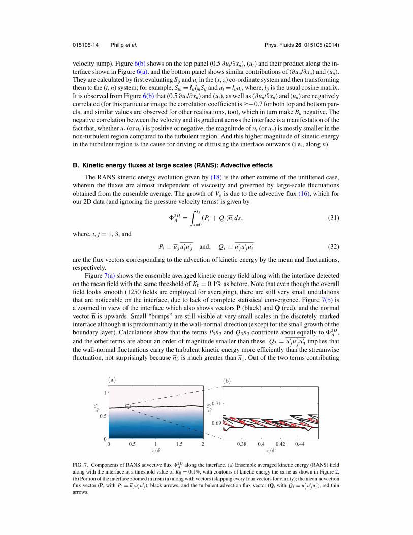
Figure 7(a) shows the ensemble averaged kinetic energy field along with the interface detectedon the mean field with the same threshold of K0 = 0.1% as before. Note that even though the overallfield looks smooth (1250 fields are employed for averaging), there are still very small undulationsthat are noticeable on the interface, due to lack of complete statistical convergence. Figure 7(b) isa zoomed in view of the interface which also shows vectors P (black) and Q (red), and the normalvector n is upwards. Small “bumps” are still visible at very small scales in the discretely markedinterface although n is predominantly in the wall-normal direction (except for the small growth of theboundary layer). Calculations show that the terms P3n3 and Q3n3 contribute about equally to �2D
A ,and the other terms are about an order of magnitude smaller than these. Q3 = u′
j u′j u
′3 implies that
the wall-normal fluctuations carry the turbulent kinetic energy more efficiently than the streamwisefluctuation, not surprisingly because n3 is much greater than n1. Out of the two terms contributing
0 0.5 1 1.5 20
0.5
1
z/δ
x/δ
(a)
0.38 0.4 0.42 0.44
0.69
0.71
z/δ
x/δ
(b)
FIG. 7. Components of RANS advective flux �2DA along the interface. (a) Ensemble averaged kinetic energy (RANS) field
along with the interface at a threshold value of K0 = 0.1%, with contours of kinetic energy the same as shown in Figure 2.(b) Portion of the interface zoomed in from (a) along with vectors (skipping every four vectors for clarity); the mean advectionflux vector (P, with Pi ≡ u j u′
i u′j ), black arrows; and the turbulent advection flux vector (Q, with Qi ≡ u′
j u′j u
′i ), red thin
arrows.
015105-15 Philip et al. Phys. Fluids 26, 015105 (2014)
to P3n3, u1u′1u′
3n3 dominates, implying that mean streamwise velocity in conjunction with theReynolds stress at the interface also contribute significantly to the entrainment. It is interesting tonote that the inviscid analysis of Reynolds21 shows that there is a “jump” across the interface inthe Reynolds stress which is equal to the product of the mean normal velocity across the interfaceand the “jump” in the mean tangential velocity. This shows that P3 can in turn be related to themean effect. However, we show that fluctuations also have an equally important role to play in thelarge-scale entrainment via the term Q3.
C. Kinetic energy fluxes at intermediate (filtered) scales: Viscous/advective effects
For a multi-scale analysis of the entrainment, the PIV database is coarse-grained using spatialfiltering and contributions from viscous and advective fluxes are quantified. The velocity field andnonlinear terms are filtered with a kernel G�(x), such that, e.g., ui = ∫
ui (x − x′)G�(x′)d2x′. Inthe present case, we employ a 2D box-filter G�(x, z) = 1/�2 if |x|, |z| < �/2 and G�(x, z) = 0otherwise.
For the PIV data, 2D surrogates of LES advective (24) and viscous (25) fluxes are definedrespectively as
�2DA� =
∫ s f
s=0Ai ni ds and, �2D
ν� =∫ s f
s=0Bi ni ds, (33)
where, the LES advective flux vector A j ≡ (1/2)(u j ui ui − u j ui ui ), and the corresponding viscous
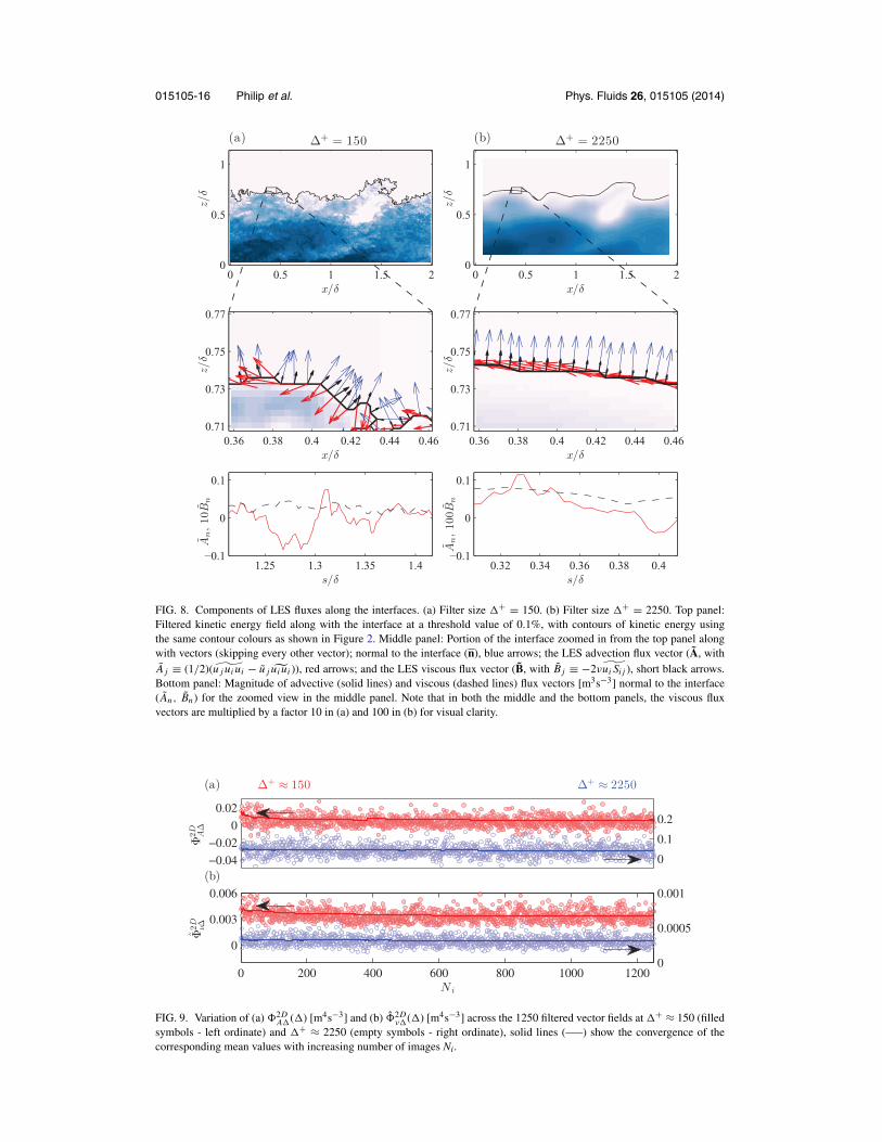
flux vector B j ≡ −2ν˜ui Si j . Figures 8(a) and 8(b) show two examples of filtering at filter sizes of�+ = 150 and 2250, respectively. We recall that the spacing between the vectors is about 50 viscousunits. The effect of filtering is clearly visible in the top panel, with small scale features smoothed outfor higher filter size. The viscous flux vector has essentially the same characteristics for both filtersizes (as noticed in connection with the unfiltered case); B is mostly facing outwards in the directionof n, even though the magnitudes have dropped drastically with filtering. On the other hand, theadvective flux vectors A have much higher magnitudes than B, and are generally directed in thenegative x-direction. For smaller filter sizes (cf., Figure 8(a), middle panel) A has no preferentialalignment with n; for larger filter sizes (cf., Figure 8(b), middle panel) A is more uniform and stillnot aligned with n; however, now A might seem better correlated with n simply because the interface
is smoother. In fact, (1/ ls)∫
(A · n) ds (where, ˆ denotes the unit vector) increases from 0.01 to 0.03
for �+ increasing from 150 to 2250 for the data in Figure 8, whereas, (1/ ls)∫
(B · n) ds ≈ 0.9 forboth filter sizes.
Consequently, advective and “resolved” viscous fluxes contribute differently to the entrainment(or in this case, to the outward growth of the interface) at various scales. Advective fluxes aredictated by the large-scale features of the flow, and not by the local interface, and rely on theirlarge magnitudes (rather than alignment with local normal) to drive the interface outwards. On theother hand, viscous flux vectors are largely aligned with the local interface normally and drive theinterface, notwithstanding the fact that their magnitudes decrease with increasing filter size, thusbecoming less effective at higher �+.
Calculations of �2DA� and �2D
ν� for individual fields for the Reτ = 14 500 data are shown inFigures 9(a) and 9(b), respectively, for �+ = 150 and 2250. The convergence with Ni to theirrespective mean values occurs relatively quickly for both �2D
A� and �2Dν�. Note that the first data
points in Figure 9 correspond to the fields shown in Figure 8.
D. Comparison of unfiltered and RANS with multi-scale (LES) fluxes
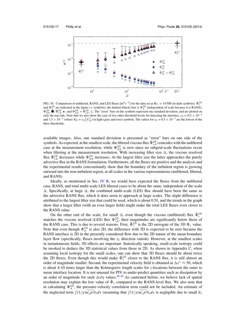
Figure 10 shows the viscous (unfiltered) flux �2Dν , the advective RANS flux �2D
A , and theindividual LES fluxes �2D
ν� and �2DA�, as well as their sum as function of filter scale, for the
Reτ = 14 500 data in dark symbols. (The lighter symbols are for different threshold levels to bediscussed below.) The dashed line represents the value of �2D
A . The data points for the unfiltered andmulti-scale fluxes are first calculated for individual images and subsequently averaged over all
015105-16 Philip et al. Phys. Fluids 26, 015105 (2014)
0 0.5 1 1.5 20
0.5
1
z/δ
x/δ
(a) Δ+ = 150
0.36 0.38 0.4 0.42 0.44 0.460.71
0.73
0.75
0.77
z/δ
x/δ
1.25 1.3 1.35 1.4−0.1
0
0.1
An,10
Bn
s/δ
0 0.5 1 1.5 20
0.5
1
z/δ
x/δ
(b) Δ+ = 2250
0.36 0.38 0.4 0.42 0.44 0.460.71
0.73
0.75
0.77
z/δ
x/δ
0.32 0.34 0.36 0.38 0.4−0.1
0
0.1
An,10
0Bn
s/δ
FIG. 8. Components of LES fluxes along the interfaces. (a) Filter size �+ = 150. (b) Filter size �+ = 2250. Top panel:Filtered kinetic energy field along with the interface at a threshold value of 0.1%, with contours of kinetic energy usingthe same contour colours as shown in Figure 2. Middle panel: Portion of the interface zoomed in from the top panel alongwith vectors (skipping every other vector); normal to the interface (n), blue arrows; the LES advection flux vector (A, withA j ≡ (1/2)(u j ui ui − u j ui ui )), red arrows; and the LES viscous flux vector (B, with B j ≡ −2ν ˜ui Si j ), short black arrows.Bottom panel: Magnitude of advective (solid lines) and viscous (dashed lines) flux vectors [m3s−3] normal to the interface( An, Bn) for the zoomed view in the middle panel. Note that in both the middle and the bottom panels, the viscous fluxvectors are multiplied by a factor 10 in (a) and 100 in (b) for visual clarity.
FIG. 9. Variation of (a) �2DA�(�) [m4s−3] and (b) �2D
ν�(�) [m4s−3] across the 1250 filtered vector fields at �+ ≈ 150 (filledsymbols - left ordinate) and �+ ≈ 2250 (empty symbols - right ordinate), solid lines (—–) show the convergence of thecorresponding mean values with increasing number of images Ni.
015105-17 Philip et al. Phys. Fluids 26, 015105 (2014)
FIG. 10. Comparison of unfiltered, RANS, and LES fluxes [m4s−3] for the data set at Reτ = 14 500 (in dark symbols). �2Dν
and �2DA are indicated in the figure (+ symbols); the dashed (black) line is �2D
A (independent of scale because it is RANS);�2D
A�, �; �2Dν�, • ; and �2D
A� + �2Dν�, �. The “error” bars on the symbols represent one standard deviation, and are plotted on
only the top-side. Note that we also show the case of two other threshold levels for detecting the interface, c0 = 0.5 × 10⁻³
and 1.5 × 10⁻³ (where K0 = c012 U 2∞) in light (grey and rose) symbols. The values for c0 = 0.5 × 10⁻³ are the lowest of the
three thresholds.
available images. Also, one standard deviation is presented as “error” bars on one side of thesymbols. As expected, at the smallest scale, the filtered viscous flux �2D
ν� coincides with the unfilteredcase at the measurement resolution, while �2D
A� is zero since no subgrid-scale fluctuations occurwhen filtering at the measurement resolution. With increasing filter size �, the viscous resolvedflux �2D
ν� decreases while �2DA� increases. At the largest filter size the latter approaches the purely
advective flux in the RANS formulation. Furthermore, all the fluxes are positive and the analysis andthe experimental results concomitantly show that the boundary of the turbulent region is growingoutward into the non-turbulent region, at all scales in the various representations (unfiltered, filtered,and RANS).
Ideally, as mentioned in Sec. IV B, we would have expected the fluxes from the unfilteredcase, RANS, and total multi-scale LES filtered cases to be about the same, independent of the scale�. Specifically, at large �, the combined multi-scale (LES) flux should have been the same asthe advective RANS flux, which it does seem to approach at large scales. The slight difference isattributed to the largest filter size that could be used, which is about 0.5δ, and the trends in the graphshow that a larger filter (with an even larger field) might make the total LES fluxes even closer tothe RANS value.
On the other end of the scale, for small �, even though the viscous (unfiltered) flux �2Dν
matches the viscous resolved (LES) flux �2Dν�, their magnitudes are significantly below those of
the RANS case. This is due to several reasons. First, �2Dν is the 2D surrogate of the 3D �ν value.
Note that even though �2DA is also 2D, the difference with 3D is expected to be zero because the
RANS interface is 2D in the presently considered flow due to the 2D nature of the mean boundarylayer flow (specifically, fluxes involving the x2 direction vanish). However, at the smallest scalesin instantaneous fields, 3D effects are important. Statistically speaking, small-scale isotropy couldbe invoked to deduce the 3D statistical values from those in 2D. As shown in Appendix C, whenassuming local isotropy for the small scales, one can show that 3D fluxes should be about twicethe 2D fluxes. Even though this would make �2D
ν closer to the RANS flux, it is still almost anorder of magnitude smaller. Second, the experimental velocity field is obtained at �x+ ≈ 50, whichis about 4-10 times larger than the Kolmogorov length scales for z-locations between the outer tomean interface location. It is not unusual for PIV to under-predict quantities such as dissipation byan order of magnitude for such �x/η values.48, 49 As cautioned before, we believe lack of spatialresolution may explain the low value of �ν compared to the RANS-level flux. We also note thatin calculating �2D
A , the pressure-velocity correlation term could not be included. An estimate ofthe neglected term
∫(1/ρ)u′
3 p′n3ds (assuming that∫
(1/ρ)u′1 p′n1ds is negligible due to small n1
015105-18 Philip et al. Phys. Fluids 26, 015105 (2014)
compared to n3) made from the DNS kinetic energy balance for a turbulent boundary layer at Reτ
= 1272 by Schlatter and Orlu50 is ≈10% of the calculated �2DA with an opposite sign.51
The effect of the threshold level on the variations in the calculated fluxes are exhibited inFigure 10 by plotting the un-averaged, filtered and RANS fluxes for c0 = 0.5 × 10⁻³ and 1.5 ×10⁻³ (recall that K0 = c0
12U 2
∞) in lighter symbols. Even though there is slight shift in the measureddistributions, the overall trend is the same.
E. Scaling of fluxes and the entrainment velocity
To understand the scaling of the fluxes the calculations similar to Sec. V D are repeated for thedatabase at Reτ = 7870 (using the same threshold value of 0.1%). The PIV velocity fields of Adrian,Meinhart, and Tomkins29 at Reτ = 2790 are also used to calculate the fluxes (even though there areonly 50 realisations available and we have to employ a threshold value of 0.15%). Results for themeasured fluxes shown in Sec. V D were in dimensional units, i.e., they were not normalised. In orderto compare results at different Reτ , it useful to define fluxes per unit interface length, accordingly,
�2Dν ≡ 1
ls�2D
ν , (34)
where ls is the total interface length of the individual fields, i.e., �2Dν is the viscous flux per unit
length. It is made non-dimensional by uτ , i.e., �2D+ν = �2D
ν /u3τ , and a similar definition is also
used for the advective flux. Normalised fluxes for Reτ = 14500, 7870, and 2790 are plotted inFigures 11(a)–11(c) with the abscissa normalised by inner, outer, and Taylor microscale (at the meaninterface location of ≈0.67δ), respectively. A reasonable collapse of �2D+
ν at the ordinate for thethree Reτ data (even though � differ by more than an order of magnitude between the differentReynolds numbers) seems to suggest that the flux per unit length does scale with u3
τ . This might notbe surprising, considering the fact that u′ (the turbulent velocity fluctuations) scale almost linearlywith uτ even as far from the wall as the interface location. The role of local fluctuating velocity inthe propagation of the interface has also been observed by Holzner et al.52 in their experiments andDNS with oscillating-grids.
Note that the inner and outer normalisation (see Figures 11(a) and 11(b), respectively) tendto collapse the small and the large �s differently. The viscous scaling is less satisfactory at all �,whereas a better collapse of large scales with outer scaling is simply because large eddies scalewith the boundary layer thickness δ. On the other hand, λT seems to collapse the data well for thelower/mid range of �. This is likely because length scales which dictate the entrainment at smallscales are of the order of Taylor microscale (e.g., da Silva and Taveira27 have shown that the radiusof the vortices which reside along the interface are comparable to the large vorticity structures andare of the order of Taylor microscale in shear-flows). The significance of λT at smaller scales and thatof δ at largest scales is also exemplified in the “mass-entrainment spectrum” presented by Chauhanet al.25 which characterizes the length scales at which the local and the total mass are entrained intothe boundary layer. As an aside, we note that the Kolmogorov length scale η+ is relatively invariantwith Reτ in the outer region of the boundary layer, and the variation in Taylor micro-scale λ+
T ismoderate.53
Finally, some observations regarding entrainment velocities are made. Recalling the requirement(from the fact that total flux is constant at any scale, see Eqs. (28) and (D7)), that v�
s S(�) is a constant,if the surface area S(�) follows fractal like scaling S(�) ∼ �2−D f with a fractal dimension ofapproximately Df = 7/3 (e.g., see, Ref. 19), then S(�) ∼ �−1/3. This should hold within a rangeof scales between an inner and outer cutoff scale. This leads to the conclusion that the averageentrainment velocity at scale � follows,
v�s (�) ∼ �1/3, (35)
consistent with inertial-range Kolmogorov scaling of transport velocities. We cannot, however, verifythis prediction since even though the surface area scales as S(�) ∼ �−1/3, the total flux (�A� + �ν�)is not observed to be independent of scale (see Figure 10) due to possibly scale-dependent effectsfrom 3D to 2D corrections and resolution issues at the smallest scales. Due to 2D measurement
015105-19 Philip et al. Phys. Fluids 26, 015105 (2014)
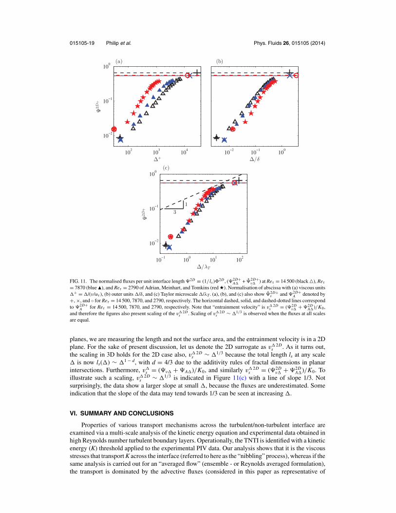
FIG. 11. The normalised fluxes per unit interface length �2D ≡ (1/ ls )�2D , (�2D+A� + �2D+
ν� ) at Reτ = 14 500 (black �), Reτ
= 7870 (blue �), and Reτ = 2790 of Adrian, Meinhart, and Tomkins (red ★). Normalisation of abscissa with (a) viscous units�+ = �/(ν/uτ ), (b) outer units �/δ, and (c) Taylor microscale �/λT. (a), (b), and (c) also show �2D+
ν and �2D+A denoted by
+, ×, and ◦ for Reτ = 14 500, 7870, and 2790, respectively. The horizontal dashed, solid, and dashed-dotted lines correspondto �2D+
A for Reτ = 14 500, 7870, and 2790, respectively. Note that “entrainment velocity” is v� 2Ds = (�2D
ν� + �2DA�)/K0,
and therefore the figures also present scaling of the v� 2Ds . Scaling of v� 2D
s ∼ �1/3 is observed when the fluxes at all scalesare equal.
planes, we are measuring the length and not the surface area, and the entrainment velocity is in a 2Dplane. For the sake of present discussion, let us denote the 2D surrogate as v� 2D
s . As it turns out,the scaling in 3D holds for the 2D case also, v� 2D
s ∼ �1/3 because the total length ls at any scale� is now ls(�) ∼ �1 − d, with d = 4/3 due to the additivity rules of fractal dimensions in planarintersections. Furthermore, v�
s = (�ν� + �A�)/K0, and similarly v� 2Ds = (�2D
ν� + �2DA�)/K0. To
illustrate such a scaling, v� 2Ds ∼ �1/3 is indicated in Figure 11(c) with a line of slope 1/3. Not
surprisingly, the data show a larger slope at small �, because the fluxes are underestimated. Someindication that the slope of the data may tend towards 1/3 can be seen at increasing �.
VI. SUMMARY AND CONCLUSIONS
Properties of various transport mechanisms across the turbulent/non-turbulent interface areexamined via a multi-scale analysis of the kinetic energy equation and experimental data obtained inhigh Reynolds number turbulent boundary layers. Operationally, the TNTI is identified with a kineticenergy (K) threshold applied to the experimental PIV data. Our analysis shows that it is the viscousstresses that transport K across the interface (referred to here as the “nibbling” process), whereas if thesame analysis is carried out for an “averaged flow” (ensemble - or Reynolds averaged formulation),the transport is dominated by the advective fluxes (considered in this paper as representative of
015105-20 Philip et al. Phys. Fluids 26, 015105 (2014)
the “engulfment” process) with negligible viscous contributions. In between, a multi-scale analysisby filtering the fields at particular length scales shows that except at the smallest and largestscales, both viscous (nibbling) and advective (engulfing) processes are active. Furthermore, theanalysis suggests that independent of the scale, the total flux should be approximately the same.Consequently, the results are consistent with “engulfment” and “nibbling” being viewed as describingthe same entrainment process, however, at the largest and smallest scales, respectively. At in-betweenlength scales both advective and nibbling contribute to the overall entrainment. We stress again thatthe equivalency between the concept of “large-scale engulfment” and the more precisely defined“advective flux” at various scales that we have assumed here may not correspond precisely to priorinterpretations or definitions of “large-scale engulfment” and this should be kept in mind.
Two-dimensional experimental data from PIV in turbulent boundary layers at Reτ of 14 500and 7870 (along with a relatively smaller data-set of Adrian, Meinhart, and Tomkins29 at Reτ =2790) are analysed to understand the specific nature of the viscous and advective fluxes operativeat the interface. At the smallest scale (describing the nibbling process), the viscous fluxes drivethe growth of the boundary layer by the work done by the viscous stresses. This is confirmedby the strong negative correlation of the normal/tangential velocities and their gradients along theinterface. Qualitatively the process of entrainment by viscous fluxes wherein the viscous flux vectoris aligned with the local interface normal remains the same at increasing scales even though theflux magnitudes decrease rapidly as the filtering scale is increased. Advective fluxes on the otherhand drive entrainment primarily due to their large magnitudes, rather than any particular alignmentwith the local interface. At large scales, the interface flattens and the local normals to the interfacebecome less random, making the alignment between the advective flux vector and local normalslightly higher. At the largest scales, where the entire entrainment is driven by advective fluxes(describing the engulfment process), two specific contributions occur equally: the mean flow andshear-stress interaction, and the advection of K due to turbulent fluctuations. The former is relatedentirely to the mean flow (due to the relation given by Reynolds,21 between shear-stress and meantangential velocity jump) and has been the one studied mostly in the literature. However, it is shownthat for entrainment the advection by turbulent fluctuations is also equally important. The multi-scaleflux calculations based on the LES filtering formalism show that with increasing scale the advectiveflux contribution becomes dominant over the (resolved) viscous contribution. As a result, for mostintermediate scales (except for the smallest), advective fluxes prevail over nibbling.
While the present PIV data provide us with sufficient information at high Reynolds numbersto describe the overall trends of each of the processes correctly, lack of spatial resolution deep intothe viscous range yields viscous nibbling fluxes that are smaller than the advective ones that operateat the large scales. Nonetheless, the transport equation clearly shows that viscous nibbling mustrise sufficiently to balance the overall entrainment flux that determines the growth of the turbulentboundary layer.
Viscous and advective fluxes are analysed at multi-scales for three different Reynolds numbersfrom two different laboratories, and collapse well when the fluxes are converted to fluxes per unitinterface length and normalised with u3
τ . This shows that uτ or the local fluctuating velocity (sincethe local fluctuating velocity in the outer region scales with uτ ) in the laboratory frame (ratherthan attached to the interface) is the appropriate velocity scale (in general agreement with Holzneret al.52). When length-scales are normalized with the Taylor scale, reasonable collapse is observedin the small/mid length scales, highlighting the importance of the Taylor scale. This may be expectedsince we recognize that the definition of the nibbling flux (Eq. (7)) involves the product of the viscousshear stress, a small-scale quantity, with the local velocity, a large-scale one. On the other hand, fluxesat larger � seem to scale with δ similar to the largest eddies in the outer region of the boundary layer.Furthermore, scaling of the entrainment velocity v�
s ∼ �1/3 derived by considering a multiscale(fractal) interface and constant flux across scales could not be verified due to under-estimation ofviscous fluxes at smaller �, however, approaches such a scaling at larger scales.
These results provide evidence at higher Reynolds numbers that interfaces in turbulence areaccompanied by transport processes that depend on scale. The results suggest that the overall rateof entrainment is determined by the large-scales but that the actual entrainment occurs physicallyat the small diffusive scales along the interface. Nevertheless, lack of sufficient spatial resolution at
015105-21 Philip et al. Phys. Fluids 26, 015105 (2014)
the smallest scales prevented us from capturing the full magnitude of the viscous fluxes and hencethe data do not yet fully prove whether once viscous fluxes are fully resolved they match the onesfrom the large scales. Nevertheless, the theoretical analysis of the energy budget and overall growthof the interface indicates that this must be the case.
ACKNOWLEDGMENTS
The authors wish to thank Dr. Kapil Chauhan and Dr. Daniel Chung for fruitful discussions,and the Australian Research Council for the financial support of this work. The visit of C.M. tothe University of Melbourne was supported by the Australian-American Fulbright CommissionSenior Scholar Fellowship and a University of Melbourne MERIT Visiting Fellowship. C.M. alsoacknowledges partial funding from the NSF (Grant No. CBET -1033942).
APPENDIX A: EFFECTS FROM IRROTATIONAL KINETIC ENERGY WITHINTHE CONTROL VOLUME Vo
Here we consider terms that appear in (8). We begin with the closed-surface integral∫∫So
(K + p
ρ
)(ui − Ui )ni d S containing the inertial terms. If we now assume that the flow out-
side the interface is mostly irrotational, we may apply the unsteady Bernoulli equation between anypoint on the boundary and the far-field, K + p/ρ = p∞/ρ − ∂φ/∂t (where φ is the velocity potential),and obtain ∫∫
So
(K + p
ρ
)(ui − Ui )ni d S ≈ −
∫∫So
(∂φ
∂t
)(ui − Ui )ni d S, (A1)
since∫∫
So(p∞/ρ)(ui − Ui )ni d S = 0 from mass conservation (
∫∫So
(ui − Ui )ni d S = 0). The closedsurface integral on the right hand side of (A1) can be written (recalling that n points inwards intoVo) as
−∫∫
So
(∂φ
∂t
)(ui − Ui )ni d S =
∫∫∫Vo
∂
∂xi
(∂φ
∂t
∂φ
∂xi
)dV =
∫∫∫Vo
(∂
∂t
∂φ
∂xi
) (∂φ
∂xi
)dV,
(A2)where we have assumed that ui − Ui = ∂φ/∂xi and used ∇2φ = 0. This leads to
−∫∫
So
(∂φ
∂t
)(ui − Ui )ni d S =
∫∫∫Vo
∂
∂xi
(∂φ
∂t
∂φ
∂xi
)dV = dKpot
Vo
dt, (A3)
where KpotVo
= ∫∫∫Vo
(1/2) (∂φ/∂xi )2 dV is the kinetic energy in the potential-flow portion of thefluctuations outside of the interface.
The other term in (8) that needs to be considered is the surface integration∫∫
SoKUi ni d S =
K0∫∫
SintU1n1d S + U1
∫∫SL
K n1d S + ∫∫SU
KU1n1d S. The integral over the interface Sint was al-ready considered in the main text, while the integral over SU vanishes since n1 = 0 there. Along SL,the inward pointing normal has n1 = 1. Along this surface K < K0 and is likely small. Consistentwith the previous reasoning we assume the fluctuations at most contain irrotational contributions.Let 〈Kpot〉L be the average value of these fluctuations along SL. Typically one expects 〈Kpot〉L � K0,especially if Kpot decays rapidly away from the interface. Combined with the arguments in the maintext leading to (10), the surface integral can be written as∫∫
So
KUi ni d S = −U1 K0dδ
dxAxy + U1〈K pot〉L
dδ
dxAxy . (A4)
Finally, if one includes explicit consideration of the irrotational portion of the kinetic energy in Vo,(10) can instead be written according to
d
dt
(KVo − Kpot
Vo
)+ (
K0 − 〈K pot〉L)
U1dδ
dxAxy = �ν − D. (A5)
015105-22 Philip et al. Phys. Fluids 26, 015105 (2014)
In other words, it can be seen that the flux �ν affects the portion of the outer kinetic energy thatis assumed to be rotational. It will have no effect on the irrotational portions, which instead can beaffected by pressure work at the interface. We note that in the analysis of the experimental databasewe always consider a frame of reference moving with the free-stream velocity (i.e., U1 = 0), andthe second term in (A5) is identically zero.
At this point, it might be interesting to have an estimate of the term d/dt(KpotV0
). To this end,we employ the expression of Phillips2 for the decay of kinetic energy in the potential region dueto random fluctuations at the interface, according to which the kinetic energy ∼h−4, where h is thedistance from the interface. It is experimentally validated by Bradshaw54 for the case of a turbulentboundary layer and the expression seems to hold even inside the intermittent region of the boundarylayer. Therefore, we consider the (potential) kinetic energy of the irrotational fluid in the controlvolume V0, which is assumed to vary like Kpot = K0(z/δ)−4, where z is the wall-normal distance.Note that at z = δ, we have the usual Kpot = K0. Hence, the total potential kinetic energy in thecontrol volume V0 per unit spanwise width (with δ = δ0 + xc, where the constant c = dδ/dx) is
KpotV0
= K0
∫ Lx
x=0
∫ h
z=δ(x)
( z
δ
)−4dzdx = K0
3
∫ Lx
x=0
(δ − δ4
h3
)dx
= K0
3
[δ0Lx + cL2
x
2− 1
5h3c
{(δ0 + cLx )5 − δ5
0
}], (A6)
where, Lx is the length of the streamwise domain under consideration, and we have taken the controlvolume to extend up to a constant height h in the z-direction. Now, δ0 is a function of time (such thatin a frame of reference moving with the free-stream velocity the boundary layer moves outwards),and dδ0/dt = U∞dδ/dx |δ0 = U∞c. This suggests that (with K0 = c0( 1
2U 2∞), c0 = 10−3),
�2Dpot+ ≡ 1
Lx u3τ
dKpotV0
dt= c0U+3
∞ c
6
[1 −
(cLx
h
)3{(
δ0
cLx+ 1
)4
−(
δ0
cLx
)4}]
. (A7)
In the present experiments for the case of Reτ = 14 500, we have c = 0.012 and U+∞ = 31.75. An
upper bound of �2Dpot+ results when we extend the volume to ∞, or in the limit h/� → ∞, andthis results in �2Dpot+ ≈ 6.4 × 10⁻². However, for a realistic and finite h, say h = 2δ, �2Dpot+ ≈ 3.2× 10⁻². These values of �2Dpot+ should be compared to the distribution of �2D+ in Figure 11, andshows that maximum of �2Dpot+ is about 5%-10% of the RANS case �2D+
A . Note that, we expect�2Dpot+ to be relatively invariant with the filter size �, since the average RANS interface and theun-averaged interface are nominally at the same z-location.
APPENDIX B: INTERFACE FOR MULTI-SCALE ANALYSIS
The interface is defined with the same threshold of K = 10−3(
12U 2
∞)
for each formalism, basedon unfiltered fields, RANS, and filtered (LES) fields. Specifically, K ≡ (1/2)(u2 + w2) for the LEScase and K ≡ (1/2)(u2 + w2) for the RANS case, in a co-ordinate system which moves with the freestream velocity (i.e., U = 0). Due to the nonlinear nature of the definition of K it is not obvious ifusing the same threshold would yield an interface which (at least visually) could be considered as thesame interface expressed at various resolutions. In this appendix, we provide empirical evidence thatindeed the basic definition and the same threshold enable us to roughly identify the same interfaceat various resolutions.
By taking a single field as an example, Figure 12 shows various ways in which K could bedefined. It shows the original interface along with three definitions of K at �+ ≈ 950: (i) Kbin
obtained by filtering the binary (T/NT) image (with the turbulent region assigned a value unity andzero otherwise, and obtaining an interface at the value of 0.5 after filtering), (ii) calculating K and
then filtering, i.e., (1/2)( ˜u2 + w2), and (iii) first filtering and then calculating K, i.e., (1/2)(u2 + w2).Out of the three, the third is the most logical definition which is extendable to any scale, and theone used in the main text. Figure 12 shows that visually they all appear similar and not far from the
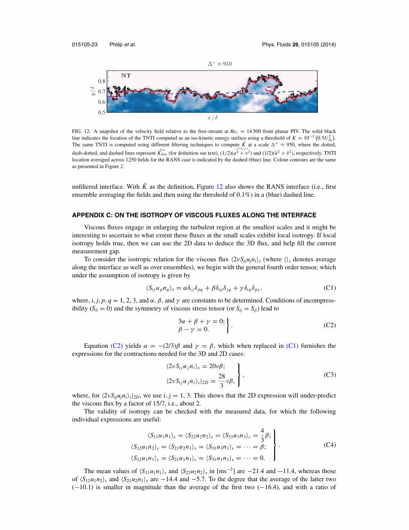
015105-23 Philip et al. Phys. Fluids 26, 015105 (2014)
FIG. 12. A snapshot of the velocity field relative to the free-stream at Reτ = 14 500 from planar PIV. The solid blackline indicates the location of the TNTI computed as an iso-kinetic energy surface using a threshold of K = 10−3
(0.5U 2∞
).
The same TNTI is computed using different filtering techniques to compute K at a scale �+ ≈ 950, where the dotted,
dash-dotted, and dashed lines represent Kbin (for definition see text), (1/2)( ˜u2 + v2) and (1/2)(u2 + v2), respectively. TNTIlocation averaged across 1250 fields for the RANS case is indicated by the dashed (blue) line. Colour contours are the sameas presented in Figure 2.
unfiltered interface. With K as the definition, Figure 12 also shows the RANS interface (i.e., firstensemble averaging the fields and then using the threshold of 0.1%) in a (blue) dashed line.
APPENDIX C: ON THE ISOTROPY OF VISCOUS FLUXES ALONG THE INTERFACE
Viscous fluxes engage in enlarging the turbulent region at the smallest scales and it might beinteresting to ascertain to what extent these fluxes at the small scales exhibit local isotropy. If localisotropy holds true, then we can use the 2D data to deduce the 3D flux, and help fill the currentmeasurement gap.
To consider the isotropic relation for the viscous flux 〈2νSijujni〉s (where 〈〉s denotes averagealong the interface as well as over ensembles), we begin with the general fourth order tensor, whichunder the assumption of isotropy is given by
〈Si j u pnq〉s = αδi jδpq + βδi pδ jq + γ δiqδpj , (C1)
where, i, j, p, q = 1, 2, 3, and α, β, and γ are constants to be determined. Conditions of incompress-ibility (Sii = 0) and the symmetry of viscous stress tensor (or Sij = Sji) lead to
3α + β + γ = 0;β − γ = 0.
}. (C2)
Equation (C2) yields α = −(2/3)β and γ = β, which when replaced in (C1) furnishes theexpressions for the contractions needed for the 3D and 2D cases:
〈2νSi j u j ni 〉s = 20νβ;
〈2νSi j u j ni 〉s |2D = 28
3νβ,
⎫⎬⎭ , (C3)
where, for 〈2νSijujni〉s|2D, we use i, j = 1, 3. This shows that the 2D expression will under-predictthe viscous flux by a factor of 15/7, i.e., about 2.
The validity of isotropy can be checked with the measured data, for which the followingindividual expressions are useful:
〈S11u1n1〉s = 〈S22u2n2〉s = 〈S33u3n3〉s = 4
3β;
〈S12u1n2〉s = 〈S21u2n1〉s = 〈S31u3n1〉s = · · · = β;
〈S12u1n1〉s = 〈S21u1n1〉s = 〈S31u1n1〉s = · · · = 0.
⎫⎪⎪⎬⎪⎪⎭ . (C4)
The mean values of 〈S11u1n1〉s and 〈S22u2n2〉s in [ms−2] are −21.4 and −11.4, whereas thoseof 〈S12u1n2〉s and 〈S21u2n1〉s are −14.4 and −5.7. To the degree that the average of the latter two(−10.1) is smaller in magnitude than the average of the first two (−16.4), and with a ratio of
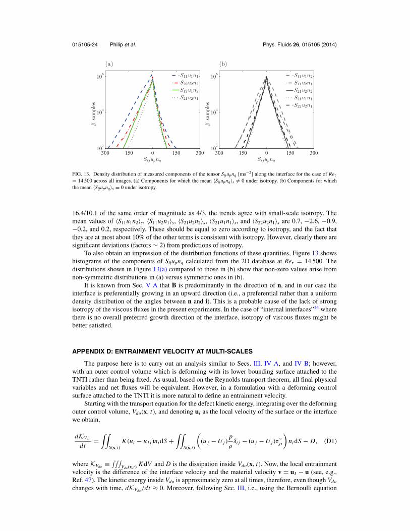
015105-24 Philip et al. Phys. Fluids 26, 015105 (2014)
−300 −150 0 150 30010
2
104
106
#sa
mpl
es
Sijupnq
(a)
S11u1n1
S22u2n2
S12u1n2
S21u2n1
−300 −150 0 150 30010
2
104
106
#sa
mpl
es
Sijupnq
(b)
S11u1n2
S11u2n1
S21u2n2
S21u1n1
S22u2n1
FIG. 13. Density distribution of measured components of the tensor Sijupnq [ms−2] along the interface for the case of Reτ
= 14 500 across all images. (a) Components for which the mean 〈Sijupnq〉s �= 0 under isotropy. (b) Components for whichthe mean 〈Sijupnq〉s = 0 under isotropy.
16.4/10.1 of the same order of magnitude as 4/3, the trends agree with small-scale isotropy. Themean values of 〈S11u1n2〉s, 〈S11u2n1〉s, 〈S21u2n2〉s, 〈S21u1n1〉s, and 〈S22u2n1〉s are 0.7, −2.6, −0.9,−0.2, and 0.2, respectively. These should be equal to zero according to isotropy, and the fact thatthey are at most about 10% of the other terms is consistent with isotropy. However, clearly there aresignificant deviations (factors ∼ 2) from predictions of isotropy.
To also obtain an impression of the distribution functions of these quantities, Figure 13 showshistograms of the components of Sijupnq calculated from the 2D database at Reτ = 14 500. Thedistributions shown in Figure 13(a) compared to those in (b) show that non-zero values arise fromnon-symmetric distributions in (a) versus symmetric ones in (b).
It is known from Sec. V A that B is predominantly in the direction of n, and in our case theinterface is preferentially growing in an upward direction (i.e., a preferential rather than a uniformdensity distribution of the angles between n and i). This is a probable cause of the lack of strongisotropy of the viscous fluxes in the present experiments. In the case of “internal interfaces”14 wherethere is no overall preferred growth direction of the interface, isotropy of viscous fluxes might bebetter satisfied.
APPENDIX D: ENTRAINMENT VELOCITY AT MULTI-SCALES
The purpose here is to carry out an analysis similar to Secs. III, IV A, and IV B; however,with an outer control volume which is deforming with its lower bounding surface attached to theTNTI rather than being fixed. As usual, based on the Reynolds transport theorem, all final physicalvariables and net fluxes will be equivalent. However, in a formulation with a deforming controlsurface attached to the TNTI it is more natural to define an entrainment velocity.
Starting with the transport equation for the defect kinetic energy, integrating over the deformingouter control volume, Vdo(x, t), and denoting uI as the local velocity of the surface or the interfacewe obtain,
dKVdo
dt=
∫∫S(x,t)
K (ui − uI i )ni dS +∫∫
S(x,t)
((u j − U j )
p
ρδi j − (u j − U j )τ
νj i
)ni dS − D, (D1)
where KVdo ≡ ∫∫∫Vdo(x,t) K dV and D is the dissipation inside Vdo(x, t). Now, the local entrainment
velocity is the difference of the interface velocity and the material velocity v = uI − u (see, e.g.,Ref. 47). The kinetic energy inside Vdo is approximately zero at all times, therefore, even though Vdo
changes with time, dKVdo/dt ≈ 0. Moreover, following Sec. III, i.e., using the Bernoulli equation
015105-25 Philip et al. Phys. Fluids 26, 015105 (2014)
K0 + p/ρ = p∞/ρ and noting that uI is non-zero only at the interface (SI) results in
K0
∫∫SI (x,t)
v · ndS ≈ �ν − D. (D2)
It is natural to define the surface averaged entrainment velocity (vs) as
vs S =∫∫
SI (x,t)v · ndS, (D3)
where, S is the total interface surface area, S ≡ ∫∫SI (x,t) dS. And in terms of these definitions and
assuming that D ≈ 0 in the V , (D2) becomes
K0vs S ≈ �ν. (D4)
This relates the entrainment rate at the smallest scales by viscous fluxes with an average entrainmentspeed at the smallest scales, vs , see also Sec. III.
Continuing in the same vein, for the RANS case (cf., Sec. IV A), we have
K0vAs S A ≈ �A, (D5)
where, vAs and SA are defined in a manner similar to (D3) however with the RANS interface
coordinate.Similarly, for the LES case (cf., Sec. IV B):
K0v�s S(�) ≈ �A� + �ν�, (D6)
and similar definitions for v�s and S(�). And since the total entrainment should be the same at small,
large, and intermediate scales, again
vs S ≈ vAs S A ≈ v�
s S(�), (D7)
in accordance with (28).
1 S. Corrsin and A. L. Kistler, “Free-stream boundaries of turbulent flows,” NACA Technical Note No. 1244 (1955).2 O. M. Phillips, “The irrotational motion outside a free boundary layer,” Proc. Camb. Phil. Soc. 51, 220 (1955).3 A. Townsend, Structure of Turbulent Shear Flow (Cambridge University Press, 1976).4 D. J. Carruthers and J. C. R. Hunt, “Momentum and scalar transport at the turbulent/non-turbulent interface of a jet,” J.
Fluid Mech. 165, 475–501 (1986).5 K. Sreenivasan and C. Meneveau, “The fractal facets of turbulence,” J. Fluid Mech. 173, 357–386 (1986).6 J. Westerweel, C. Fukushima, J. M. Pedersen, and J. C. R. Hunt, “Momentum and scalar transport at the turbulent/non-
turbulent interface of a jet,” J. Fluid Mech. 631, 199–230 (2009).7 B. B. Mandelbrot, The Fractal Geometry of Nature (W. H. Freeman, New York, 1982).8 S. Lovejoy, “Area-perimeter relation for rain and cloud areas,” Science 216, 185–187 (1982).9 F. Gouldin, K. Bray, and J. Chen, “Chemical closure model for fractal flamelets,” Combust. Flame 77, 241 (1989).
10 K. Sreenivasan, R. Ramshankar, and C. Meneveau, “Mixing, entrainment and fractal dimensions of surfaces in turbulentflows,” Proc. R. Soc. London, Ser. A 421, 79–108 (1989).
11 C. Meneveau and K. Sreenivasan, “Interface dimension in intermittent turbulence,” Phys. Rev. A 41, 2246 (1990).12 J. Mathew and A. Basu, “Some characteristics of entrainment at a cylindrical turbulence boundary,” Phys. Fluids 14,
2065–2072 (2002).13 J. Westerweel, C. Fukushima, J. M. Pedersen, and J. C. R. Hunt, “Mechanics of the turbulent-nonturbulent interface of a
jet,” Phys. Rev. Lett. 95, 174501 (2005).14 J. C. R. Hunt, I. Eames, C. B. da Silva, and J. Westerweel, “Interfaces and inhomogeneous turbulence,” Philos. Trans. R.
Soc. London, Ser. A 369, 811–832 (2011).15 M. Holzner, A. Liberzon, N. Nikitin, W. Kinzelbach, and A. Tsinober, “Small-scale aspects of flows in proximity of the
turbulent/nonturbulent interface,” Phys. Fluids 19, 071702 (2007).16 J. Philip and I. Marusic, “Large-scale eddies and their role in entrainment in turbulent jets and wakes,” Phys. Fluids 24,
055108 (2012).17 L. S. G. Kovasznay, “Structure of the turbulent boundary layer,” Phys. Fluids. 10, S25–S30 (1967).18 C. B. da Silva, R. J. N. dos Reis, and J. C. F. Pereira, “The intense vorticity structures near the turbulent/non-turbulent
interface in a jet,” J. Fluid. Mech. 685, 165–190 (2011).19 C. M. de Silva, J. Philip, K. Chauhan, C. Meneveau, and I. Marusic, “Multiscale geometry and scaling of the turbulent/non-
turbulent interface in high Reynolds number boundary layers,” Phys. Rev. Letts. 111, 044501 (2013).20 M. Khashehchi, A. Ooi, J. Soria, and I. Marusic, “Evolution of the turbulent/non-turbulent interface of an axisymmetric
turbulent jet,” Exp. Fluids 54, 1449 (2013).21 W. C. Reynolds, “Large-scale instabilities of turbulent wakes,” J. Fluid. Mech. 54, 481–488 (1972).
015105-26 Philip et al. Phys. Fluids 26, 015105 (2014)
22 C. P. Chen and R. F. Blackwelder, “Large-scale motion in a turbulent boundary layer: A study using temperature contami-nation,” J. Fluid Mech. 89, 1–31 (1978).
23 C. B. da Silva and J. C. F. Pereira, “The role of coherent vortices near the turbulent/non-turbulent interface in a planar jet,”Philos. Trans. R. Soc. London, Ser. A 369, 738–753 (2011).
24 N. Semin, V. Golub, G. Elsinga, and J. Westerweel, “Laminar superlayer in a turbulent boundary layer,” Tech. Phys. Lett.37, 1154–1157 (2011).
25 K. Chauhan, J. Philip, C. M. de Silva, N. Hutchins, and I. Marusic, “The turbulent/non-turbulent interface and entrainmentin a boundary layer,” J. Fluid. Mech. 740, 1–33 (2014).
26 M. Holzner, A. Liberzon, M. Guala, A. Tsinober, and W. Kinzelbach, “Generalized detection of a turbulent front generatedby an oscillating grid,” Exp. Fluids 41, 711–719 (2006).
27 C. B. da Silva and R. R. Taveira, “The thickness of the turbulent/nonturbulent interface is equal to the radius of the largevorticity structures near the edge of the shear layer,” Phys. Fluids 22, 121702 (2010).
28 M. Holzner and B. Luthi, “Laminar superlayer at the turbulence boundary,” Phys. Rev. Lett. 106, 134503 (2011).29 R. J. Adrian, C. D. Meinhart, and C. D. Tomkins, “Vortex organization in the outer region of the turbulent boundary layer,”
J. Fluid. Mech. 422, 1–54 (2000).30 C. M. de Silva, K. A. Chauhan, C. H. Atkinson, N. A. Buchmann, N. Hutchins, J. Soria, and I. Marusic, “Implementation
of large scale PIV measurements for wall bounded turbulence at high Reynolds numbers,” in Proceedings of the 18thAustralasian Fluid Mechanics Conference, Vol. 18, edited by P. A. Brandner, and B. W. Pearce (Launceston, Australia,2012), pp. 308–311.
31 T. B. Hedley and J. F. Keffer, “Turbulent/non-turbulent decisions in an intermittent flow,” J. Fluid Mech. 64, 625–644(1974).
32 R. R. Prasad and K. R. Sreenivasan, “Scalar interfaces in digital images of turbulent flows,” Exp. Fluids. 7, 259–264 (1989).33 H. J. Catrakis and P. E. Dimotakis, “Mixing in turbulent jets: Scalar measures and isosurface geometry,” J. Fluid. Mech.
317, 369–406 (1996).34 H. J. Catrakis, R. Aguirre, and J. Ruiz-Plancarte, “Area-volume properties of fluid interfaces in turbulence: Scale-local
self-similarity and cumulative scale dependence,” J. Fluid Mech. 462, 245–254 (2002).35 N. D. Sandham, M. G. Mungal, J. E. Broadwell, and W. C. Reynolds, “Scalar entrainment in the mixing layer,” in
Proceedings of the Summer Program 1988 (Center for Turbulence Research, Stanford University, Stanford, CA, 1988),pp. 69–76.
36 D. Bisset, J. C. R. Hunt, and M. M. Rogers, “The turbulent/non-turbulent interface bounding a far wake,” J. Fluid Mech.451, 383–410 (2002).
37 C. B. da Silva, “The behavior of subgrid-scale models near the turbulent/nonturbulent interface in jets,” Phys. Fluids 21,081702 (2009).
38 J. Jimenez, S. Hoyas, M. P. Simens, and Y. Mizuno, “Turbulent boundary layers and channels at moderate Reynoldsnumbers,” J. Fluid Mech. 657, 335–360 (2010).
39 R. K. Anand, B. J. Boersma, and A. Agrawal, “Detection of turbulent/non-turbulent interface for an axisymmetric turbulentjet: Evaluation of known criteria and proposal of a new criterion,” Exp. Fluids 47, 995–1007 (2009).
40 G. Heckstead, “Hot-wire measurements in a plane turbulent jet,” J. Appl. Mech. 32, 721–734 (1965).41 A. J. Adrian and J. Westerweel, Particle Image Velocimetry (Cambridge University Press, 2011).42 U. Piomelli, P. Moin, and J. Ferziger, “Model consistency in large eddy simulation of turbulent channel flows,” Phys.
Fluids 31, 1884 (1988).43 S. Pope, Turbulent Flows (Cambridge University Press, 2000).44 S. Liu, C. Meneveau, and J. Katz, “On the properties of similarity subgrid-scale models as deduced from measurements in
a turbulent jet,” J. Fluid Mech. 275, 83 (1994).45 B. Tao, J. Katz, and C. Meneveau, “Statistical geometry of subgrid-scale stresses determined from holographic particle
image velocimetry measurements,” J. Fluid Mech. 457, 35–78 (2002).46 J. Chen, C. Meneveau, and J. Katz, “Scale interactions of turbulence subjected to a straining-relaxation-destraining cycle,”
J. Fluid Mech. 562, 123–150 (2006).47 M. van Reeuwijk and M. Holzner, “The turbulence boundary of a temporal jet,” J. Fluid. Mech. 739, 257–275 (2013).48 P. Saarenrinne, M. Piirto, and H. Eloranta, “A correction method for measuring turbulence kinetic energy dissipation rate
by PIV,” Meas. Sci. Technol. 12, 1904–1910 (2001).49 T. Tanaka and J. K. Eaton, “A correction method for measuring turbulence kinetic energy dissipation rate by PIV,” Exp.
Fluids 42, 893–902 (2007).50 P. Schlatter and R. Orlu, “Assessment of direct numerical simulation data of turbulent boundary layers,” J. Fluid. Mech.
659, 116–126 (2010).51 From the kinetic energy balance provided by Schlatter and Orlu,50 profiles of (1/ρ)∂(u′
3 p′)/∂y and 1/2∂(u3ui ui )/∂y areobtained, and integrated in the wallnormal direction with their values estimated at about y/δ99 ≈ 0.9, which is adapted toour situation.
52 M. Holzner, B. Luthi, A. Tsinober, and W. Kinzelbach, “Acceleration, pressure and related quantities in the proximity ofthe turbulent/nonturbulent interface,” J. Fluid. Mech. 639, 153–165 (2009).
53 I. Marusic and R. A. Adrian, “Eddies and scales of wall turbulence,” in Ten Chapters in Turbulence, edited by P.A.Davidson,Y. Kaneda, and K.R.Sreenivasan (Cambridge University Press, 2012).
54 P. Bradshaw, “Irrotational fluctuations near a turbulent boundary layer,” J. Fluid. Mech. 27, 209–230 (1967).