Multiscale Analysis of Complex Time Series

by Scale Dependent Lyapunov Exponent

Jianbo Gao

Department of Electrical & Computer EngineeringUniversity of Florida, Gainesville

gao@ece.ufl.edu

1

Outline

� Motivations� Scale Dependent Lyapunov Exponent (SDLE)

— Theory & computation

� Theoretical aspects of SDLE

– Classification of complex motions

– Distinguishing chaos from noise

– Characterizing large scale orderly motions

– Coping with nonstationarity

� Applications

� Concluding remarks

2

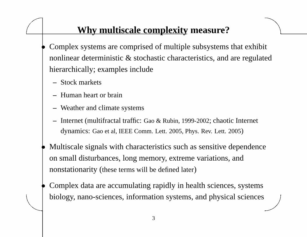
Why multiscale complexity measure?� Complex systems are comprised of multiple subsystems that exhibit

nonlinear deterministic & stochastic characteristics, and are regulated

hierarchically; examples include

– Stock markets

– Human heart or brain

– Weather and climate systems

– Internet (multifractal traffic: Gao & Rubin, 1999-2002; chaotic Internet

dynamics: Gao et al, IEEE Comm. Lett. 2005, Phys. Rev. Lett. 2005)

� Multiscale signals with characteristics such as sensitive dependence

on small disturbances, long memory, extreme variations, and

nonstationarity (these terms will be defined later)

� Complex data are accumulating rapidly in health sciences, systems

biology, nano-sciences, information systems, and physical sciences

3

How to effectively analyze complex data?� Highly desired: simultaneously characterize different behaviors of

the data on the entire or a wide range of scales resolvable by the data

� Is it possible to use existing theories synergistically for this purpose?

� Extremely difficult, if not impossible

—How to identify relevant scales to determine which theories to use?

—How to distinguish low-dimensional chaos from noise?

� Existing multiscale measures

� �

ε

�

τ

�

-entropy: Gaspard & Wang, 1993;

finite size Lyapunov exponent: Aurell et al. 1997; multiscale entropy

analysis: Costa et al. 2002, 2005

�

cannot satisfy our need

� Need a new readily computable measure to– cope with nonstationarity– effectively characterize structured and random aspects of the data– unify existing complexity measures

4

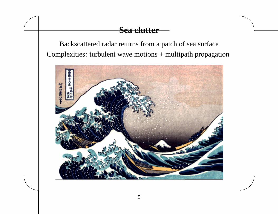
Sea clutter

Backscattered radar returns from a patch of sea surface

Complexities: turbulent wave motions + multipath propagation

5

Significance and Challenges of sea clutter modeling� Sea clutter analysis is an important theoretical problem; may shed

light on the nature of air-sea interaction

� Target detection within sea clutter is an important engineering

problem (related to coastal and national security, navigation safety,

and environmental monitoring) (Hu, Gao et al. 2005, 2006)

� Whether sea clutter is chaotic or not is still a hot issue

(Haykin et al. 1997, 1999, 2001; Gao & Yao 1999, 2000; Noga 1998, Cowper &

Mulgrew 99, Davies 2004, McDonald & Damini 2004)

� Data are highly nonstationary, naive Fourier analysis or chaos

analysis is not very useful; data are not simple random fractals

6

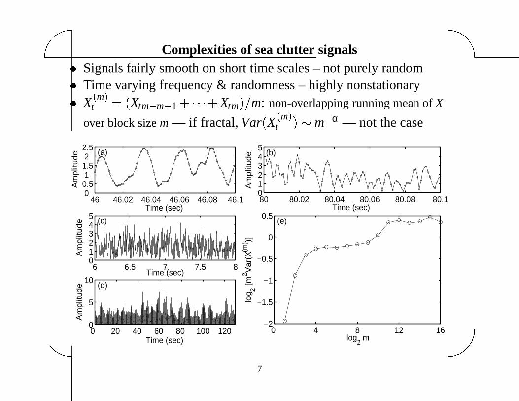
Complexities of sea clutter signals� Signals fairly smooth on short time scales – not purely random

� Time varying frequency & randomness – highly nonstationary

� X � m �t � � Xtm� m � 1� � � �� Xtm � m: non-overlapping running mean of X

over block size m — if fractal, Var � X � m �

t �� m� α — not the case

46 46.02 46.04 46.06 46.08 46.10

0.51

1.52

2.5

Time (sec)

Am

plit

ud

e

80 80.02 80.04 80.06 80.08 80.1012345

Time (sec)

Am

plit

ud

e

6 6.5 7 7.5 8012345

Time (sec)

Am

plit

ud

e

0 20 40 60 80 100 1200

5

10

Time (sec)

Am

plit

ud

e

0 4 8 12 16−2

−1.5

−1

−0.5

0

0.5

log2 m

log

2 [

m2V

ar(

X(m

) )]

(a) (b)

(c)

(d)

(e)

7

Heart rate variability (HRV) analysis� HRV is an important dynamical variable of the cardiovascular

function

� Most salient feature: spontaneous fluctuation, even without the

presence of environmental perturbations

� HRV is related to various cardiovascular disorders

� Modeled as a fractal (1 f ) process (Goldberger, Peng, Stanley, &

coworkers) — to show this, data were manually segmented to remove

parts that do not conform to fractal analysis

� The parameter from fractal analysis cannot perfectly distinguish

healthy subjects from those with cardiac diseases

� Unknown whether cardiac dynamics are chaotic; Chaos control of

fibrillation is not particularly effective

8

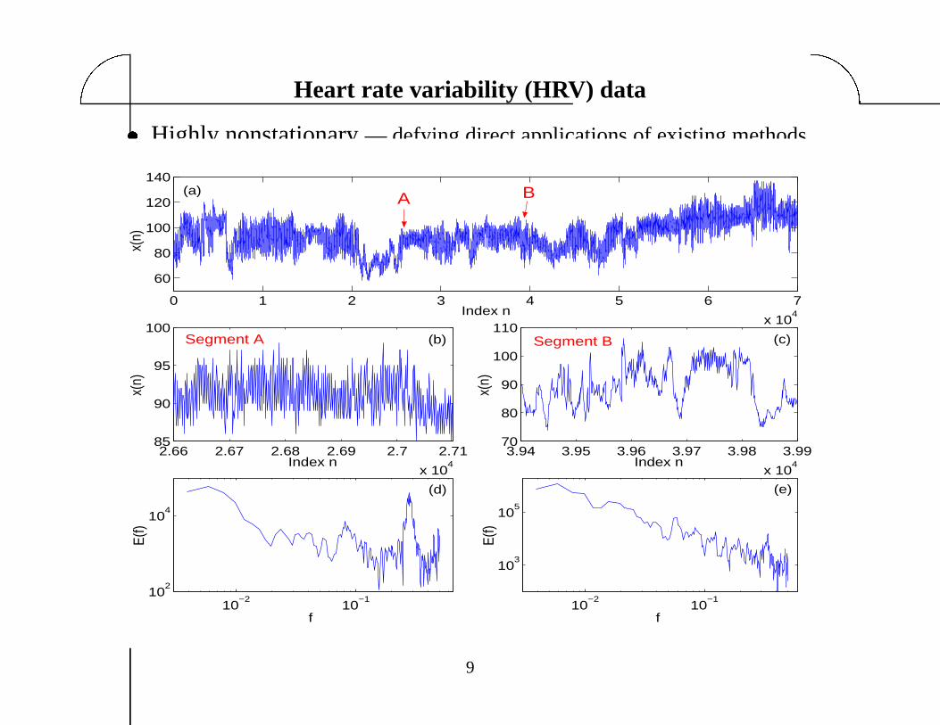
Heart rate variability (HRV) data� Highly nonstationary — defying direct applications of existing methods

0 1 2 3 4 5 6 7

x 104

60

80

100

120

140

Index n

x(n)

2.66 2.67 2.68 2.69 2.7 2.71

x 104

85

90

95

100

Index n

x(n)

3.94 3.95 3.96 3.97 3.98 3.99

x 104

70

80

90

100

110

Index n

x(n)

10−2

10−1

102

104

f

E(f)

10−2

10−1

103

105

f

E(f)

A B (a)

(b) (c)

(d) (e)

Segment A Segment B

9

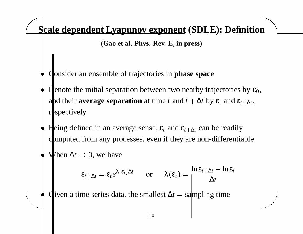
Scale dependent Lyapunov exponent (SDLE): Definition(Gao et al. Phys. Rev. E, in press)

� Consider an ensemble of trajectories in phase space

� Denote the initial separation between two nearby trajectories by ε0,

and their average separation at time t and t� ∆t by εt and εt � ∆t ,

respectively

� Being defined in an average sense, εt and εt � ∆t can be readily

computed from any processes, even if they are non-differentiable

� When ∆t � 0, we have

εt � ∆t � εteλ � εt � ∆t or λ � εt � � lnεt � ∆t� lnεt

∆t

� Given a time series data, the smallest ∆t � sampling time

10

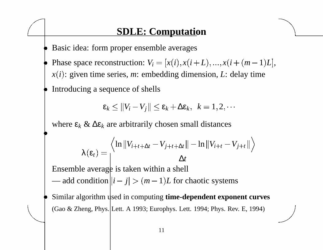
SDLE: Computation� Basic idea: form proper ensemble averages

� Phase space reconstruction: Vi � � x � i � � x � i� L � � � � � � x � i� � m� 1 � L � ,x � i � : given time series, m: embedding dimension, L: delay time

� Introducing a sequence of shells

εk � � Vi� Vj � � εk� ∆εk � k � 1 � 2 � � � �

where εk & ∆εk are arbitrarily chosen small distances

�

λ � εt � � �

ln � Vi � t � ∆t� Vj � t � ∆t � � ln � Vi � t� Vj � t � �

∆tEnsemble average is taken within a shell— add condition � i� j � � m� 1 � L for chaotic systems

� Similar algorithm used in computing time-dependent exponent curves

(Gao & Zheng, Phys. Lett. A 1993; Europhys. Lett. 1994; Phys. Rev. E, 1994)

11

Classifications of complex motions

Types of motions considered:

� Chaotic motions

– Low-dimensional deterministic chaos

– Noisy chaos

– Noise-induced chaos — without noise, motion is regular

(Gao et al. Phys. Rev. Lett. 1999, 2002; Hwang & Gao Phys. Rev. E 2000)

� 1 f β processes

� α-stable Levy processes

� Stochastic oscillations

� Complex motions with multiple scaling behaviors

12

Basics of chaos theory� Chaos is also called strange attractor

� Being an attractor, trajectories in the phase space are bounded

� Being strange, nearby trajectories diverge exponentially fast:

dr dr0eλ1t , λ1: the largest positive Lyapunov exponent

—Sensitive dependence on initial conditions

� Kolmogorov-Sinai entropy = sum of positive Lyapunov exponent(s)

� A strange attractor typically is a fractal — non-integral dimension

� Multifractal nature of chaos: the attractor may be partitioned into

many interwoven subsets, each subset has its fractal dimension, and

its weight in the original attractor is well defined

13

SDLE λ � ε � for chaos, noisy chaos, & noise-induced chaos� Chaos: λ � ε � � const � largest positive Lyapunov exponent �

� Noisy chaos & noise-induced chaos: λ � ε � � γ lnε on small scales

� (i) Stochastic Lorenz (63’) system(ii) Noisy logistic mapxn � 1 � µxn � 1� xn �� Pn � 0 � xn � 1 � µ � 3 � 74, σPn

� 0 � 002—without noise, motion is periodic — Noise-induced chaos

−1.5 −1 −0.50.5

1

1.5

2

2.5

ε

λ(ε)

−2 −1.5 −1 −0.5 00

0.1

0.2

0.3

0.4

0.5

0.6

0.7

ε

λ(ε)

D = 0D = 1D = 2D = 3D = 4

(a) Lorenz (b) Logistic

(1): slope = 0.28

(2): slope = 0

log10

log10

14

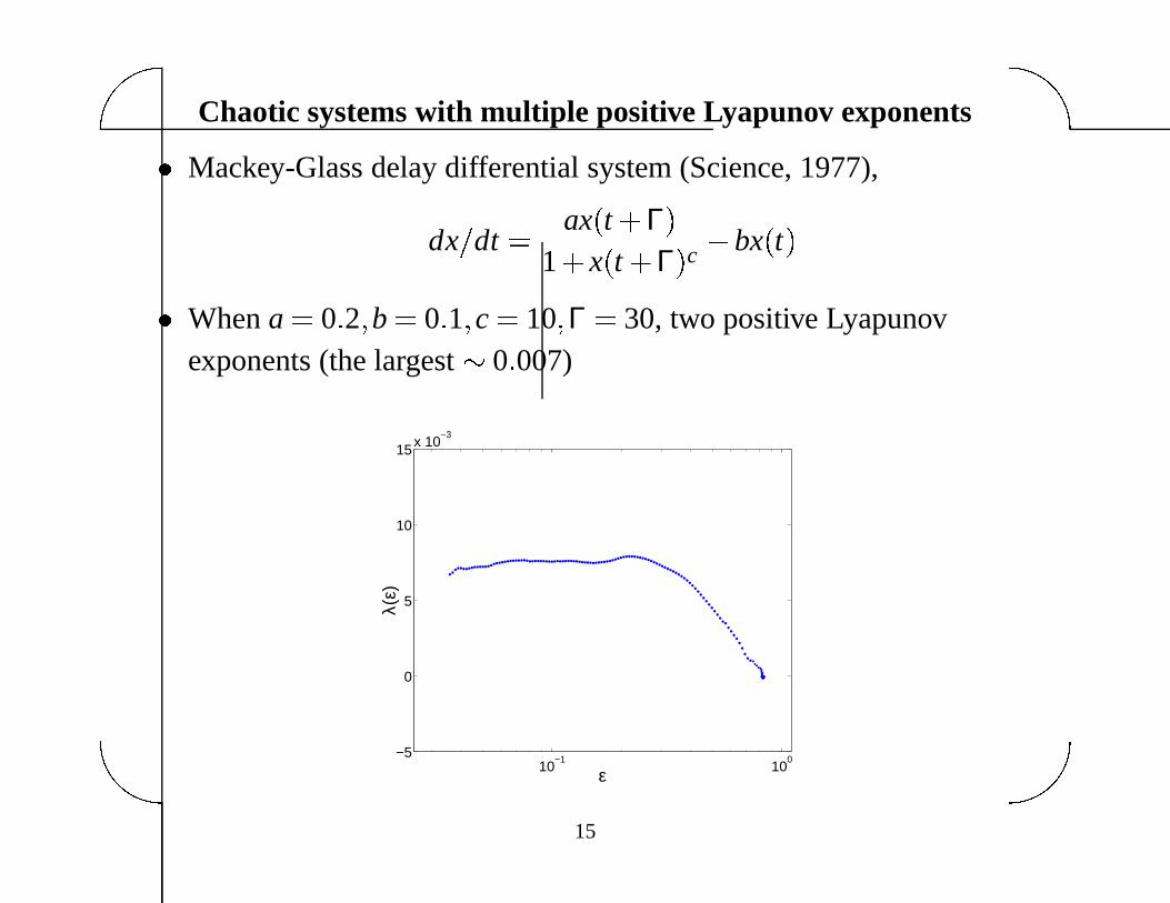
Chaotic systems with multiple positive Lyapunov exponents� Mackey-Glass delay differential system (Science, 1977),

dx dt � ax � t� Γ �

1� x � t� Γ � c

� bx � t �

� When a � 0 � 2 � b � 0 � 1 � c � 10 � Γ � 30, two positive Lyapunovexponents (the largest 0 � 007)

10−1

100−5

0

5

10

15x 10−3

ε

λ(ε)

15

1

�

f β processes� Ubiquitous in science and engineering

— music, turbulence, DNA sequence, human cognition, coordination,

posture, visual perception, Internet traffic, device noise, etc.

(Gao et al. IEEE Intell. Sys. 2005; JBB 2005; Cog. Proc. 2006; Nucleic Acids Res. 2006)

� Data

�

xt �

: variance scales as t2H , where β � 2H� 1

� Increment process�

zt � xt � 1� xt �

: power spectral density f� � 2H� 1 � ,autocorrelation r � k � k2H� 2

� k � ∞

� H: Hurst parameter

1 2 � H � 1: long memory (long-range-dependence (LRD))

H � 1 2: standard Brownian motion

0 � H � 1 2: anti-persistence

� Estimation of H: topic of active research (Gao et al. Phys. Rev. E 2006)

16

Basic math models for 1 f β processes� Fractional Brownian motion (fBm) BH � t �

– Generalization of Brownian motion (Bm)

– Gaussian process with mean 0 & stationary increments

– Variance

E � � BH � t � �

2

� � t2H

– Power spectral density

f

� � 2H � 1 �

� ON/OFF intermittency

– Power-law distributed ON/OFF train

– P � X � x �� x� µ

� 0 � µ � 2

– H � � 3� µ � 2

– Infinite variance; also infinite mean when 0 � µ � 1

17

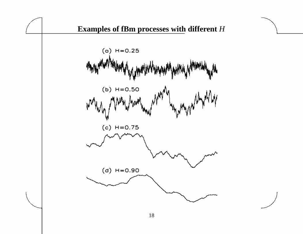
Examples of fBm processes with different H

18

Power-law scaling of λ � ε � for 1 f β processes

Can prove λ � ε � Hε� 1

�

H

−2.5 −2 −1.5−2.5

−2

−1.5

−1

−0.5

0

ε

λ(ε)

−2 −1.5 −1

−2

−1.5

−1

−0.5

ε

µ = 2.0µ = 1.6µ = 1.2

H = 0.33H = 0.50H = 0.70

(a) fBm (b) ON/OFF

(1) slope = 3.02

(2) slope = 2.04

(3)slope = 1.45

(1) slope = 1.98

(2) slope = 1.42

(3)slope = 1.10

log10

log10

log 10

log 10

λ(ε

)

19

Stable laws and Levy processes� Stable laws: distributions for the sum of independent random variables

(RV’s) & those being summed have the same functional form

� Characteristic function for the distribution of a “standard” stable RV:

ΦZ � u � � E � ejuZ

� ��

��

exp �� � u �

α

� 1� jβ tan � πα 2 � sign � u � � � α �� 1

exp �� � u �

α

� 1� jβ 2π log � u � sign � u � � � α � 1 �

where 0 � α � 2: stability index; � 1 � β � 1: skewness parameter; sign:

sign function ( � 1

�

0

�

1 depending on whether u � 0

�

� 0

�

� 0)

� In the case of strictly stable,

∑ni 1 Yi

d� n1

�

αY � nVarY � n2�

αVarY � 0 � α � 2

� α � 2: normal distribution; 0 � α � 2: heavy-tailed, P � X � x �� x� α

� Generalized central limit theorem: each stable law = attractor ofthe sum of independent RV’s with infinite variance

20

Levy processes� Levy flights: random processes consisting of many independent

steps, each step being characterized by a stable law, and consuming

a unit time regardless of its length — H � 1 2

� Symmetric Levy flights: β � 0

� Levy walks: sampled from Levy flights with a uniform speed;

each step takes time proportional to its length

— the increment process similar to power-law ON/OFF train

� A symmetric α� stable Levy flight is 1 α self-similar

� Broad applications of Levy statistics: economics, fluid mechanics,

device physics, ecology, art, etc.

21

Power-law scaling of λ � ε � for Levy flights

Can prove λ � ε � 1α ε� α — α plays the role of 1 H

4000 4500 5000 5500

1.9

2

2.1

2.2

x 104

−4 −3.5 −3−1.6

−1.2

−0.8

−0.4(a) (b)

slope = 1.01 A

B

x(n)

x(n+

1)

log 10

λ(ε

)

log10

ε

22

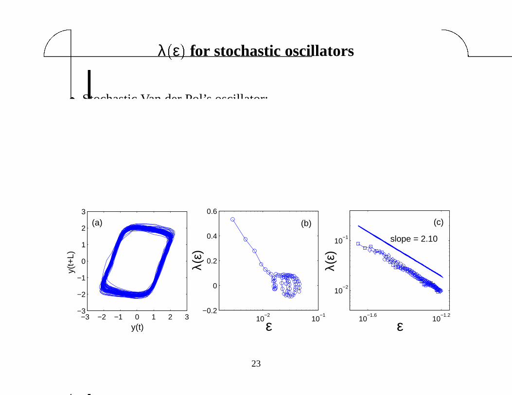
λ � ε � for stochastic oscillators� Stochastic Van der Pol’s oscillator:

dx dt � y� D1η1 � t � � dy dt � � � x2� 1 � y� x� D2η2 � t �

� λ � ε � � lnε, when � m� 1 � L is small

� λ � ε � ε� 1

�

H� H 1 2, when � m� 1 � L is large

−3 −2 −1 0 1 2 3−3

−2

−1

0

1

2

3

y(t)

y(t+

L)

10−2

10−1

−0.2

0

0.2

0.4

0.6

ε 10−1.6

10−1.2

10−2

10−1

ε

slope = 2.10

λ(ε)

λ(ε)

(a) (b) (c)

23

Stochastic oscillations: H not necessary 1/2� Pathological tremor: involuntary, approximately rhythmic, and roughly

sinusoidal movement of parts of the body

— often H 1 2 (Gao & Tung, 2000; Gao 2002)

� Karman vortex street: When Re � 137, H 1 2; When Re increases,H decreases (Lin et al. 1993; Gao 1997; Gao et al. 1999)

Left (Lim, University of Melbourne); Right: atmospheric Karman vortexstreet off Selkirk Island off the coast of Chile

24

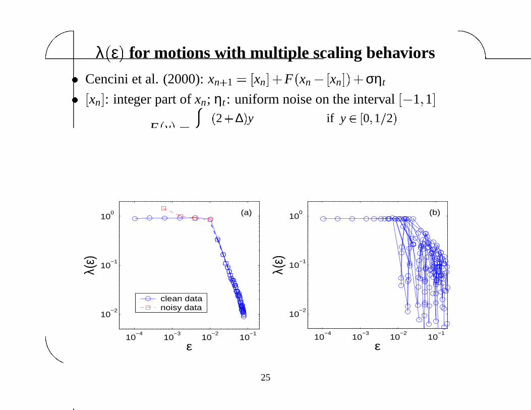
λ � ε � for motions with multiple scaling behaviors� Cencini et al. (2000): xn � 1 � � xn �� F � xn� � xn � �� σηt

� � xn � : integer part of xn; ηt : uniform noise on the interval �� 1 � 1 �

F � y � � �

2 � ∆

�

y if y � � 0 �

1 � 2

�

�

2 � ∆

�

y ��

1 � ∆

�

if y �

�

1 � 2

�

1 �

� λ1 � ln � 2� ∆ � ; � xn � introduces a random walk on integer grids— imagine a baby learning to walk

10−4

10−3

10−2

10−1

10−2

10−1

100

λ(ε)

ε10

−410

−310

−210

−1

10−2

10−1

100

ε

λ(ε)

clean datanoisy data

(a) (b)

25

Distinguishing chaos from noise� Popular test for chaos:

Positive Lyapunov exponent + non-integral fractal dimension

� Chaos in brain, heart, sea clutter, ...

� Counter-example: a 1 f 2H � 1 process with Hurst parameter H has afractal dimension 1 H and a converging K2 entropy

� Running on a wild beach, hunting for the beast of chaos(adapted from Broomhead & King 1988):“Here is a footprint”,“Here is another”...Turning around, found those are but their own footprints!

� Key: to classify various types of motions; to identify different scaleranges where different types of motions are manifested

� SDLE gets both done!

26

Characterizing large scale orderly motions by the SDLE� Defining and characterizing large scale orderly motions, such as

oscillatory ones, is a significant issue in many disciplines of science

� Hidden frequency phenomenon:

Fourier analysis of one variable

�

say x

�

t

� �

may not suggest any oscillatory

motions, while that of another variable

�

say z

�

t

� �

may

� How to reveal the hidden frequency? — Reconstruct a phase space

using x � t � to get information about z � t � , then get a 1-D signal

� Existing methods

— Ortega (1996): density method;

— Chern et al. (1998): singular value decomposition

� Our approach: Take Fourier transform of the limiting scale, ε∞

� Our method is more effective, because of scale-isolation

27

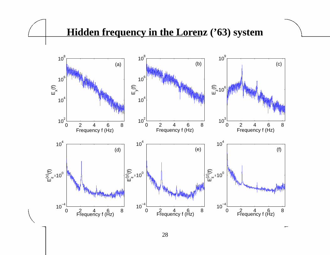
Hidden frequency in the Lorenz (’63) system

0 2 4 6 810

2

104

106

108

Frequency f (Hz)

Ex(f

)

0 2 4 6 810

2

104

106

108

Frequency f (Hz)E

y(f)

0 2 4 6 810

3

106

109

Frequency f (Hz)

Ez(f

)0 2 4 6 8

10−4

100

104

Frequency f (Hz)

E(x

)ε ∞

(f)

0 2 4 6 810

−4

100

104

Frequency f (Hz)

E(y

)ε ∞

(f)

0 2 4 6 810

−4

100

104

Frequency f (Hz)E

(z)

ε ∞

(f)

(a) (b) (c)

(d) (e) (f)

28

Coping with nonstationarity� Many real world data are nonstationary

— HRV, economic time series, etc.

� HRV, economic data, etc., are often modeled as 1 f 2H � 1; however,

poor scaling is usually observed when data are analyzed by standardfractal analysis methods

� Two sources of poor fractal scaling

– “Outliers”: whose effect is to shift the 1 f β downward or upward

at randomly chosen time instances by an arbitrary amount

— type 1 nonstationarity

– Oscillatory events: whose effect is to concatenate or superimpose

oscillatory components (on)to a 1 f β process at randomly chosen

time intervals — type 2 nonstationarity

� Still good scaling with SDLE

29

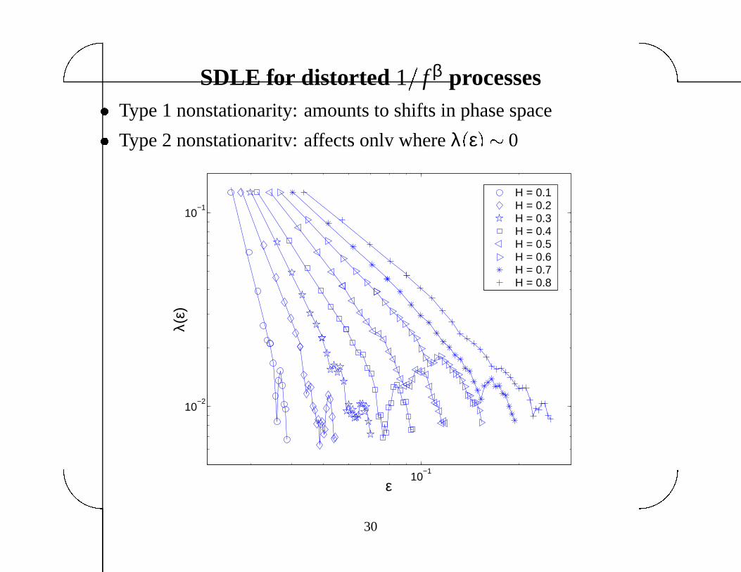
SDLE for distorted 1

�

f β processes� Type 1 nonstationarity: amounts to shifts in phase space

� Type 2 nonstationarity: affects only where λ � ε � 0

10−1

10−2

10−1

ε

λ(ε)

H = 0.1H = 0.2H = 0.3H = 0.4H = 0.5H = 0.6H = 0.7H = 0.8

30

Applications� Electroencephalogram (EEG) analysis

� Analysis of heart rate variability (HRV)

� Sea clutter modeling and target detection within sea

clutter

� Economic time series analysis

31

Analysis of EEG� EEG signals provide a wealth of information about brain dynamics,

especially related to cognitive processes and pathologies of the brainsuch as epileptic seizures

� Whether EEG is chaotic or not is still a big issue

� A number of complexity measures from information theory, chaostheory, and random fractal theory have been used to analyze EEGsignals

� These theories have different foundations � difficult to compareamong studies based on different complexity measures

� Explore the relation between SDLE & other complexity measures byanalyzing windowed EEG data for the purpose of epileptic seizureprediction/detection

32

Complexity measures for EEG� Information theory: Lempel-Ziv (LZ) complexity

(major compression scheme in Unix systems; asymptotically approaches

Shannon entropy; also closely related to Kolmogorov-Chaitin complexity)

� Chaos theory:

– Lyapunov exponent (LE), computed by Wolf’s algorithm;a length scale is needed to perform normalization

– Correlation dimension D2 & correlation entropy K2:computed by Grassberger-Procaccia’s algorithm

C

�

m

�

ε

�

�

1N2

N

∑i � j � 1

θ�

ε � � Vi � Vj � ��� εD2 e

� mLτK2

– Variants of K2: approximate entropy, sample entropy

– Permutation entropy (Cao, Tung, Gao, Phys. Rev. E 2004)

� Random fractal theory: Hurst parameter H; H � q � from multifractal

33

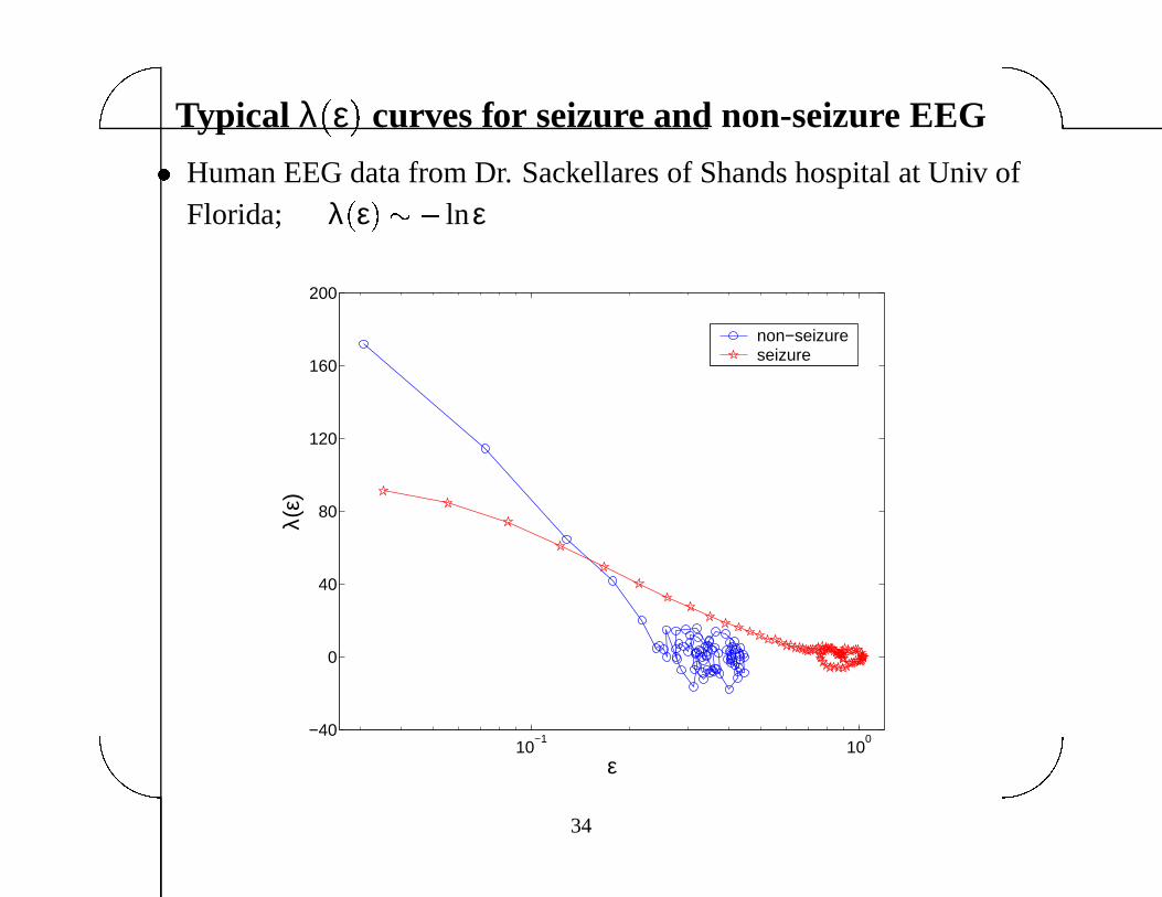
Typical λ � ε � curves for seizure and non-seizure EEG� Human EEG data from Dr. Sackellares of Shands hospital at Univ of

Florida; λ � ε � � lnε

10−1

100

−40

0

40

80

120

160

200

ε

λ(ε)

non−seizureseizure

34

Complexity measures for EEG

0 1 2 3 4 520

100

180

λ smal

l−ε(t

)

0 1 2 3 4 5

10

20

30

λ larg

e−ε(t

)

0 1 2 3 4 54

12

20

λ 1(t)

0 1 2 3 4 50

60

120

K2(t

)

0 1 2 3 4 51

2

3

4

D2(t

)

0 1 2 3 4 50.2

0.6

1

H(t

)

Time t (hour)

(a) SDLE (small scale)

(b) SDLE (large scale)

(c) Lyapunov exponent

(d) Correlation entropy

(f) DFA

(e) Correlation dimension

� λsmall� ε � t � & λlarge� ε � t � :reciprocal

� K2, Approximate, sample,

permutation entropy, LZ

λsmall� ε � t �

� D2 � t � λsmall� ε � t �

—puzzling but can be resolved

� λ1 � t � � H � t � λlarge� ε � t �

—puzzling but can be resolved� Scale-mixing blurs fea-

tures useful for seizure

prediction/detection

35

SDLE for HRV data� PhysioNet: 18 datasets for healthy subjects, 15 datasets for subjects

with congestive heart failure (CHF), a life-threatening disease

� Dimension of the dynamics of the cardiovascular system appears tobe lower for healthy than for pathological subjects— Cardiac chaos, if does exist, is more likely to be found in heathy subjects

100.7

100.8

100.9

0

0.05

0.1

0.15

0.2

0.25

ε10

0.610

0.7−0.05

0

0.05

0.1

λ(ε)

ε

(a) (b)

λ(ε)

36

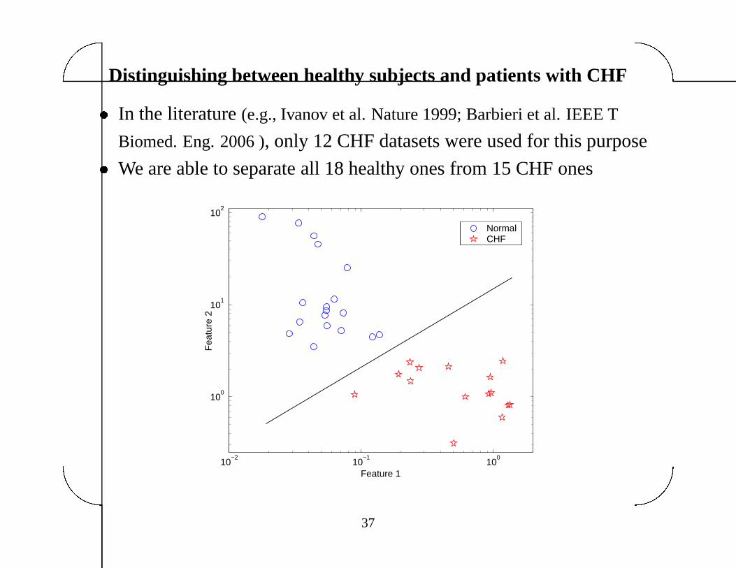
Distinguishing between healthy subjects and patients with CHF� In the literature (e.g., Ivanov et al. Nature 1999; Barbieri et al. IEEE T

Biomed. Eng. 2006 ), only 12 CHF datasets were used for this purpose

� We are able to separate all 18 healthy ones from 15 CHF ones

10−2

10−1

100

100

101

102

Feature 1

Fea

ture

2

NormalCHF

37

Sea clutter modeling & target detection within sea clutter� 400 datasets, measured with wave height 0 � 8� 3 � 8 m, winds 0� 90

km/hr, were obtained from Prof. Simon Haykin of McMaster Univ

� Target: spherical block of styrofoam of size 1 m, wrapped with wire mesh

� Small ε, λ � ε � � � γ lnε;Large ε, λ � ε � ε� 1

�

H (not shown here, see Hu, Gao et al. 2005, 2006)

10−0.6

10−0.1

−0.02

0.04

0.1

0.16

λ(ε)

ε0 5 10 15

0.4

0.6

0.8

1

1.2

Bin number

γ

Without targetWith target

(a) (b)

Primary target bin

38

Can economic time series be modeledby low-dimensional noisy chaos?

� Controversial issue in economics since late 1980’s

� Shintani & Linton (2003, 2004), Hommes & Manzan (2005):

Analyzed real & simulated economic time series using the neural

network based Lyapunov exponent estimator

� Found that largest Lyapunov exponent is negative

� Suggested that world economy may not be characterized by

low-dimensional chaos

� Kolmogorov-Sinai entropy = sum of positive Lyapunov exponents

If negative, then simple regular economic dynamics

� Economy is anything but simple !

39

Analysis of a chaotic asset pricing model� Brock and Hommes asset pricing model (BH, 1998): a nonlinear map

of the form:

xt � F � xt� 1 � xt� 2 � xt� 3 �� σηt

� xt : deviation of price of the risky asset from its benchmark

fundamental value; σηt : noise

� Model contains a number of parameters

� For suitable choice of the parameter values, the model exhibits

chaotic dynamics

� Hommes and Manzan (HM, 2005):

Lyapunov exponent becomes negative when noise is increased

� We study two parameter sets: BH, 1998; HM, 2005

40

λ � ε � curves for the asset pricing model� Why LE � 0 for strong stochastic forcing?

� Neural network: global optimization to minimize error between thegiven time series and the estimated � involves a scale parameter ε�

� To get non-null result, large ε� is chosen with λ � ε� � � 0

10−7

10−5

10−3

10−1

101

−0.2

0

0.2

0.4

0.6

0.8

ε10

−410

−210

0

0

0.2

0.4

0.6

ε

λ(ε)

σ = 0σ = 10−5

σ = 10−4

σ = 10−3

σ = 10−2

σ = 0.1

σ = 0σ = 10−5

σ = 10−4

σ = 10−3

σ = 10−2

σ = 0.1

(a) (b)

λ(ε)

41

Analysis of foreign exchange rate� No indication of noisy chaotic behavior

� Belong to 1 f 2H � 1 process; majority : H 1 2, but H � 1 2 or

H 1 2 also possible

� Deviation from H 1 2 might indicate economic/political ties

between two nations

0 2000 4000 6000 80000.5

1

1.5

2

Exc

hang

e ra

te

10−2

10−2

10−1

λ(ε)

0 1000 2000 30000

5

10

15E

xcha

nge

rate

10−2

10−2

10−1

λ(ε)

0 2000 4000 6000500

1000

1500

2000

Time

Exc

hang

e ra

te

10−3

10−2

10−2

10−1

ε

λ(ε)

H = 0.49 ± 0.04

H = 0.43 ± 0.10

H = 0.66 ± 0.05

(a) (b)

(c) (d)

(e) (f)

42

Concluding remarks� Introduced a new multiscale complexity measure, the SDLE

� Considered issues of classification of complex motions, distinction

between chaos & noise, nonstationarity, hidden frequency

� Considered various applications — results are all promising

� What is next?

– Meaning of γ in λ � ε � � γ lnε? —Rate of loss of information

– Spatialtemporal systems

– Information flow & directional control

(neuroscience — cortical control of advanced prostheses;

systems biology — cell cycle control, cell-cell communication)

� Contact me if you are interested in our methods and codes!

43

Joint work with

Jing Hu: University of Florida

Wen-wen Tung: Purdue University

Yinhe Cao: Biosieve

Partially supported by DOE & ARO

Jing Hu will graduate soon. She is now looking for a good job

44