Multirate notes

ECE-700 Multirate Notes

Phil Schniter

March 27, 2006

1 Fundamentals of Multirate Signal Processing

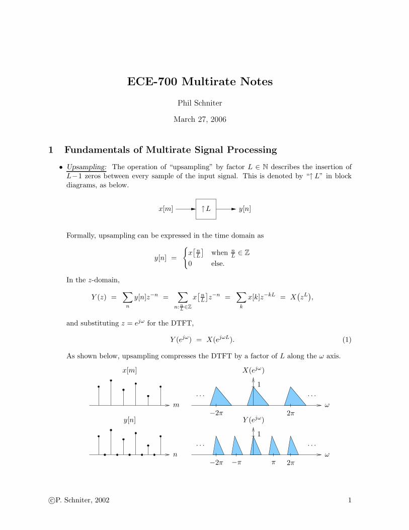
• Upsampling: The operation of “upsampling” by factor L ∈ N describes the insertion ofL−1 zeros between every sample of the input signal. This is denoted by “↑L” in blockdiagrams, as below.

x[m] y[n]↑L

Formally, upsampling can be expressed in the time domain as

y[n] =

x[

nL

]when n

L ∈ Z

0 else.

In the z-domain,

Y (z) =∑

n

y[n]z−n =∑

n: nL∈Z

x[

nL

]z−n =

∑

k

x[k]z−kL = X(zL),

and substituting z = ejω for the DTFT,

Y (ejω) = X(ejωL). (1)

As shown below, upsampling compresses the DTFT by a factor of L along the ω axis.

1

1

x[m]

y[n]

X(ejω)

Y (ejω)

−2π

−2π 2π

2π−π π

· · ·

· · ·

· · ·

· · ·

n

m

ω

ω

c©P. Schniter, 2002 1

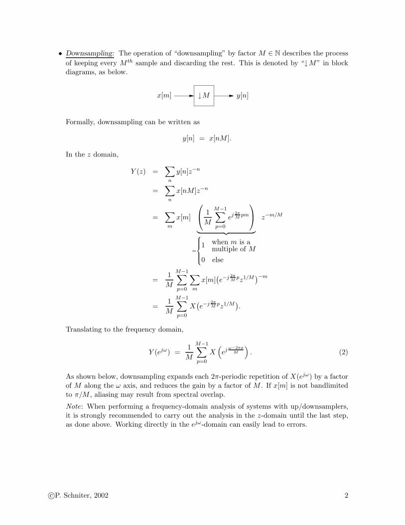
• Downsampling: The operation of “downsampling” by factor M ∈ N describes the process

of keeping every M th sample and discarding the rest. This is denoted by “↓M” in blockdiagrams, as below.

x[m] y[n]↓M

Formally, downsampling can be written as

y[n] = x[nM ].

In the z domain,

Y (z) =∑

n

y[n]z−n

=∑

n

x[nM ]z−n

=∑

m

x[m]

1

M

M−1∑

p=0

ej 2πM

pm

︸︷︷︸

=

8

>

>

>

<

>

>

>

:

1 when m is amultiple of M

0 else

z−m/M

=1

M

M−1∑

p=0

∑

m

x[m](e−j 2π

Mpz1/M

)−m

=1

M

M−1∑

p=0

X(e−j 2π

Mpz1/M

).

Translating to the frequency domain,

Y (ejω) =1

M

M−1∑

p=0

X(

ej ω−2πp

M

)

. (2)

As shown below, downsampling expands each 2π-periodic repetition of X(ejω) by a factorof M along the ω axis, and reduces the gain by a factor of M . If x[m] is not bandlimitedto π/M , aliasing may result from spectral overlap.

Note: When performing a frequency-domain analysis of systems with up/downsamplers,it is strongly recommended to carry out the analysis in the z-domain until the last step,as done above. Working directly in the ejω-domain can easily lead to errors.


1

1

1/M

x[m]

y[n]

X(ejω)

X(ejω/M )

Y (ejω)

−4π

−4π

−4π

−2π

−2π

−2π

2π

2π

2π

4π

4π

4π

· · ·· · ·

· · ·· · ·

· · ·· · ·m

n ω

ω

ω

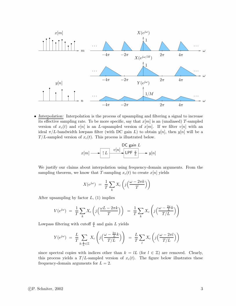
• Interpolation: Interpolation is the process of upsampling and filtering a signal to increaseits effective sampling rate. To be more specific, say that x[m] is an (unaliased) T -sampledversion of xc(t) and v[n] is an L-upsampled version of x[m]. If we filter v[n] with anideal π/L-bandwidth lowpass filter (with DC gain L) to obtain y[n], then y[n] will be aT/L-sampled version of xc(t). This process is illustrated below.

x[m]v[n]

y[n]LPF πL

DC gain L

↑L

We justify our claims about interpolation using frequency-domain arguments. From thesampling theorem, we know that T -sampling xc(t) to create x[n] yields

X(ejω) =1

T

∑

k

Xc

(

j(ω − 2πk

T

))

After upsampling by factor L, (1) implies

V (ejω) =1

T

∑

k

Xc

(

j(ωL − 2πk

T

))

=1

T

∑

k

Xc

(

j(ω − 2π

L k

T/L

))

Lowpass filtering with cutoff πL and gain L yields

Y (ejω) =L

T

∑

k: kL∈Z

Xc

(

j(ω − 2π

L k

T/L

))

=L

T

∑

l

Xc

(

j(ω − 2πl

T/L

))

since spectral copies with indices other than k = lL (for l ∈ Z) are removed. Clearly,this process yields a T/L-sampled version of xc(t). The figure below illustrates thesefrequency-domain arguments for L = 2.


x[m]v[n]

y[n]

|X(ejω)| |V (ejω)| |Y (ejω)|

000 πππ π2 2π2π2π

11 2

LPF π2

DC gain 2

↑2

• Application of Interpolation—Oversampling in CD Players:

The digital audio signal on a CD is a 44.1 kHz sampled representation of a continuoussignal with bandwidth 20 kHz. With a standard ZOH-DAC, the analog reconstructionfilter would have passband edge at 20 kHz and stopband edge at 24.1 kHz. (See the figurebelow.) With such a narrow transition band, this would be a difficult (and expensive)filter to build.

ωΩ2π

Ω2π

0 0 020k 20k

24.1k

44.1k 44.1kπ 2π

|X(ejω)| |Xz(jΩ)| |Hr(jΩ)|

If digital interpolation is used prior to reconstruction, the effective sampling rate can beincreased and the reconstruction filter’s transition band can be made much wider, resultingin a much simpler (and cheaper) analog filter. The figure below illustrates the case ofinterpolation by 4. The reconstruction filter has passband edge at 20 kHz and stopbandedge at 156.4 kHz, resulting in a much wider transition band and therefore an easier filterdesign.

ωΩ2π

Ω2π

0 0 0

20k

20k 156.4k 156.4k

176.4k176.4kπ 2π

|X(ejω)| |Xz(jΩ)| |Hr(jΩ)|

• Decimation: Decimation is the processing of filtering and downsampling a signal to de-crease its effective sampling rate, as illustrated below. The filtering is employed to preventaliasing that might otherwise result from downsampling.

x[m]v[m]

y[n]LPF πM

DC gain 1

↓M

To be more specific, say thatxc(t) = xl(t) + xb(t),

where xl(t) is a lowpass component bandlimited to 12MT Hz and xb(t) is a bandpass com-

ponent with energy between 12MT and 1

2T Hz. If sampling xc(t) with interval T yields an


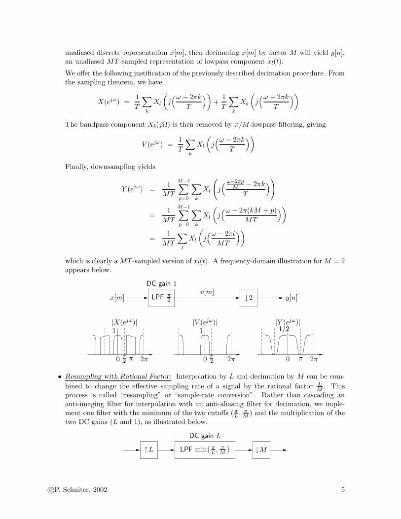
unaliased discrete representation x[m], then decimating x[m] by factor M will yield y[n],an unaliased MT -sampled representation of lowpass component xl(t).

We offer the following justification of the previously described decimation procedure. Fromthe sampling theorem, we have

X(ejω) =1

T

∑

k

Xl

(

j(ω − 2πk

T

))

+1

T

∑

k

Xb

(

j(ω − 2πk

T

))

The bandpass component Xb(jΩ) is then removed by π/M -lowpass filtering, giving

V (ejω) =1

T

∑

k

Xl

(

j(ω − 2πk

T

))

Finally, downsampling yields

Y (ejω) =1

MT

M−1∑

p=0

∑

k

Xl

(

j( ω−2πp

M − 2πk

T

))

=1

MT

M−1∑

p=0

∑

k

Xl

(

j(ω − 2π(kM + p)

MT

))

=1

MT

∑

l

Xl

(

j(ω − 2πl

MT

))

which is clearly a MT -sampled version of xl(t). A frequency-domain illustration for M = 2appears below.

x[m]v[m]

y[n]

|X(ejω)| |V (ejω)| |Y (ejω)|

000 ππ π2

π2 2π2π2π

11 1/2

LPF π2

DC gain 1

↓2

• Resampling with Rational Factor: Interpolation by L and decimation by M can be com-

bined to change the effective sampling rate of a signal by the rational factor LM . This

process is called “resampling” or “sample-rate conversion”. Rather than cascading ananti-imaging filter for interpolation with an anti-aliasing filter for decimation, we imple-ment one filter with the minimum of the two cutoffs ( π

L , πM ) and the multiplication of the

two DC gains (L and 1), as illustrated below.

↑L ↓MLPF min πL , π

M

DC gain L


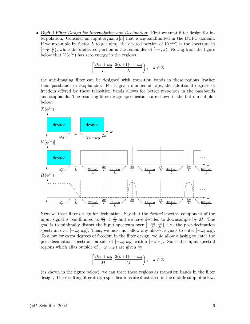
• Digital Filter Design for Interpolation and Decimation: First we treat filter design for in-terpolation. Consider an input signal x[n] that is ω0-bandlimited in the DTFT domain.If we upsample by factor L to get v[m], the desired portion of V (ejω) is the spectrum in[− π

L , πL

), while the undesired portion is the remainder of [−π, π). Noting from the figure

below that V (ejω) has zero energy in the regions

[2kπ + ω0

L,2(k+1)π − ω0

L

)

, k ∈ Z

the anti-imaging filter can be designed with transition bands in these regions (ratherthan passbands or stopbands). For a given number of taps, the additional degrees offreedom offered by these transition bands allows for better responses in the passbandsand stopbands. The resulting filter design specifications are shown in the bottom subplotbelow.

|X(ejω)|

|V (ejω)|

|H(ejω)|

ω

ω

ω0

0

0

π 2π2π−ω0ω0

ω0

L

ω0

L

πL

πL 2π−ω0

L

2π−ω0

L

2πL

2πL

2π+ω0

L

2π+ω0

L

3πL

3πL

4π−ω0

L

4π−ω0

L

4πL

4πL

4π+ω0

L

4π+ω0

L

5πL

5πL

6π−ω0

L

6π−ω0

L

desired

desireddesired

. . .

. . .

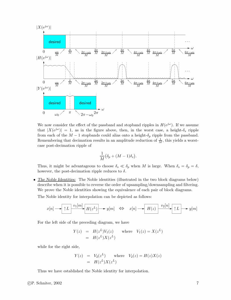
Next we treat filter design for decimation. Say that the desired spectral component of theinput signal is bandlimited to ω0

M < πM and we have decided to downsample by M . The

goal is to minimally distort the input spectrum over[−ω0

M , ω0

M

), i.e., the post-decimation

spectrum over [−ω0, ω0). Thus, we must not allow any aliased signals to enter [−ω0, ω0).To allow for extra degrees of freedom in the filter design, we do allow aliasing to enter thepost-decimation spectrum outside of [−ω0, ω0) within [−π, π). Since the input spectralregions which alias outside of [−ω0, ω0) are given by

[2kπ + ω0

M,2(k+1)π − ω0

M

)

, k ∈ Z

(as shown in the figure below), we can treat these regions as transition bands in the filterdesign. The resulting filter design specifications are illustrated in the middle subplot below.


|X(ejω)|

|Y (ejω)|

|H(ejω)|

ω

ω

ω0

0

0 ω0

M

ω0

M

πM

πM

2π−ω0

M

2π−ω0

M

2πM

2πM 2π+ω0

M

2π+ω0

M

3πM

3πM

4π−ω0

M

4π−ω0

M

4πM

4πM

4π+ω0

M

4π+ω0

M

5πM

5πM

6π−ω0

M

6π−ω0

M

ω0π

2π−ω02π

desireddesired

desired

. . .

. . .

We now consider the effect of the passband and stopband ripples in H(ejω). If we assumethat |X(ejω)| = 1, as in the figure above, then, in the worst case, a height-δs ripplefrom each of the M − 1 stopbands could alias onto a height-δp ripple from the passband.Remembering that decimation results in an amplitude reduction of 1

M , this yields a worst-case post-decimation ripple of

1

M

(δp + (M − 1)δs

).

Thus, it might be advantageous to choose δs ≪ δp when M is large. When δs = δp = δ,however, the post-decimation ripple reduces to δ.

• The Noble Identities: The Noble identities (illustrated in the two block diagrams below)describe when it is possible to reverse the order of upsampling/downsampling and filtering.We prove the Noble identities showing the equivalence of each pair of block diagrams.

The Noble identity for interpolation can be depicted as follows:

↑L↑L x[n]x[n]v1[m] v2[n]

y[m]y[m] H(z)H(zL) ⇔

For the left side of the preceding diagram, we have

Y (z) = H(zL)V1(z) where V1(z) = X(zL)

= H(zL)X(zL)

while for the right side,

Y (z) = V2(zL) where V2(z) = H(z)X(z)

= H(zL)X(zL)

Thus we have established the Noble identity for interpolation.


The Noble identity for decimation can be depicted as follows:

↓M ↓Mx[n] x[n]v1[m] v2[n]

y[m] y[m]H(z) H(zM )⇔

For the left side of the preceding diagram, we have

Y (z) = H(z)V1(z)

= H(z)1

M

M−1∑

k=0

X(e−j 2πM

kz1

M )

while for the right side,

Y (z) =1

M

M−1∑

k=0

V2(e−j 2π

Mkz

1

M ) where V2(z) = X(z)H(zM )

=1

M

M−1∑

k=0

X(e−j 2πM

kz1

M )H(e−j 2πM

MkzMM )

= H(z)1

M

M−1∑

k=0

X(e−j 2πM

kz1

M )

Thus we have established the Noble identity for decimation. Note that the impulse responseof H(zL) is the L-upsampled impulse response of H(z).

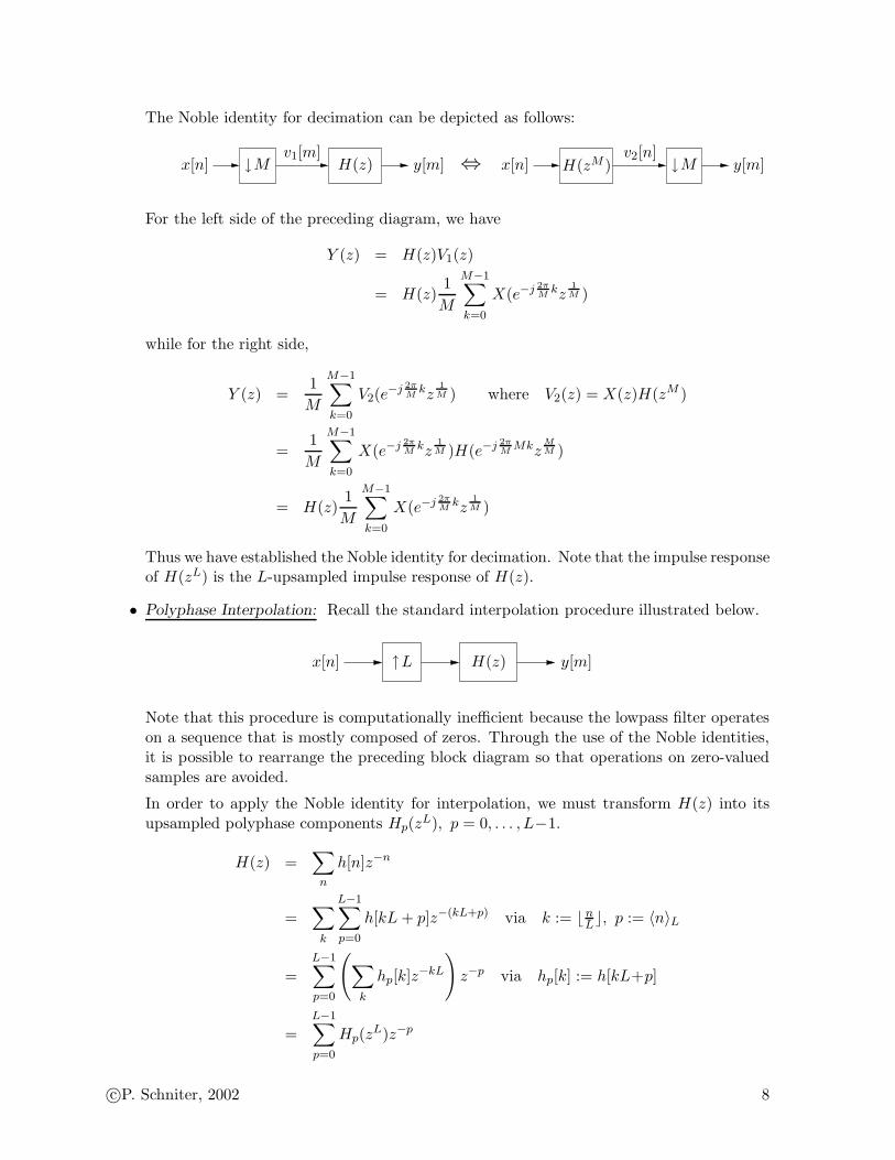
• Polyphase Interpolation: Recall the standard interpolation procedure illustrated below.

x[n] y[m]H(z)↑L

Note that this procedure is computationally inefficient because the lowpass filter operateson a sequence that is mostly composed of zeros. Through the use of the Noble identities,it is possible to rearrange the preceding block diagram so that operations on zero-valuedsamples are avoided.

In order to apply the Noble identity for interpolation, we must transform H(z) into itsupsampled polyphase components Hp(z

L), p = 0, . . . , L−1.

H(z) =∑

n

h[n]z−n

=∑

k

L−1∑

p=0

h[kL + p]z−(kL+p) via k := ⌊nL⌋, p := 〈n〉L

=L−1∑

p=0

(∑

k

hp[k]z−kL

)

z−p via hp[k] := h[kL+p]

=L−1∑

p=0

Hp(zL)z−p


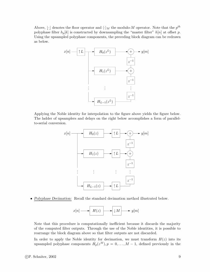
Above, ⌊·⌋ denotes the floor operator and 〈·〉M the modulo-M operator. Note that the pth

polyphase filter hp[k] is constructed by downsampling the “master filter” h[n] at offset p.Using the upsampled polyphase components, the preceding block diagram can be redrawnas below.

x[n] y[m]

+

+

z−1

z−1

z−1

......

...

H0(zL)

H1(zL)

HL−1(zL)

↑L

Applying the Noble identity for interpolation to the figure above yields the figure below.The ladder of upsamplers and delays on the right below accomplishes a form of parallel-to-serial conversion.

x[n] y[m]

+

+

z−1

z−1

z−1

......

......

H0(z)

H1(z)

HL−1(z) ↑L

↑L

↑L

• Polyphase Decimation: Recall the standard decimation method illustrated below.

x[n] y[m]H(z) ↓M

Note that this procedure is computationally inefficient because it discards the majorityof the computed filter outputs. Through the use of the Noble identities, it is possible torearrange the block diagram above so that filter outputs are not discarded.

In order to apply the Noble identity for decimation, we must transform H(z) into itsupsampled polyphase components Hp(z

M ), p = 0, . . . ,M − 1, defined previously in the


context of polyphase interpolation.

H(z) =∑

n

h[n]z−n

=∑

k

M−1∑

p=0

h[kM + p]z−kM−p via k := ⌊ nM ⌋, p := 〈n〉M

=

M−1∑

p=0

(∑

k

hp[k]z−kM

)

z−p via hp[k] := h[kM+p]

=

M−1∑

p=0

Hp(zM )z−p

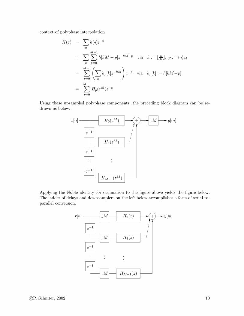
Using these upsampled polyphase components, the preceding block diagram can be re-drawn as below.

x[n] y[m]+

z−1

z−1

z−1

......

H0(zM )

H1(zM )

HM−1(zM )

↓M

Applying the Noble identity for decimation to the figure above yields the figure below.The ladder of delays and downsamplers on the left below accomplishes a form of serial-to-parallel conversion.

x[n] y[m]+

z−1

z−1

z−1

...... ...

H0(z)

H1(z)

HM−1(z)↓M

↓M

↓M


• Computational Savings of Polyphase Interpolation/Decimation: Assume that we designFIR LPF H(z) with N taps, requiring N multiplies per output. For standard decimationby factor M , we have N multiplies per intermediate sample and M intermediate samplesper output, giving NM multiplies per output.

For polyphase decimation, we have NM multiplies per branch and M branches, giving a

total of N multiplies per output. The assumption of NM multiplies per branch follows from

the fact that h[n] is downsampled by M to create each polyphase filter. Thus, we concludethat the standard implementation requires M times as many operations as its polyphasecounterpart. (For decimation we count multiplies per output, rather than per input, toavoid confusion, since only every M th input produces an output.)

From this result, it appears that the the number of multiplications required by polyphasedecimation is independent of the decimation rate M . However, it should be rememberedthat the length N of the π

M -lowpass FIR filter H(z) will typically be proportional to M .This is suggested by, e.g., the Kaiser FIR-length approximation formula

N ≈−10 log10(δpδs) − 13

2.324∆ω

where ∆ω is the transition bandwidth in radians, and δp and δs are the passband andstopband ripple levels. Recall that, to preserve a fixed signal bandwidth, the transitionbandwidth ∆ω will be linearly proportional to the cutoff π

M , so that N will be linearlyproportional to M . In summary, polyphase decimation by factor M requires N multipliesper output, where N is the filter length, and where N is linearly proportional to M .

Using similar arguments for polyphase interpolation, we could find essentially the sameresult. Polyphase interpolation by factor L requires N multiplies per input, where N isthe filter length, and where N is linearly proportional to the interpolation factor L. (Forinterpolation we count multiplies per input, rather than per output, to avoid confusion,since M outputs are generated in parallel.)

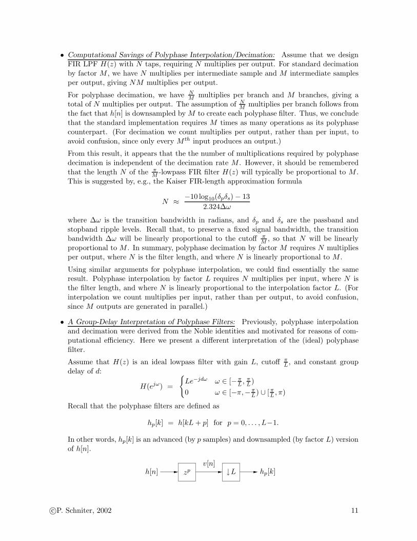
• A Group-Delay Interpretation of Polyphase Filters: Previously, polyphase interpolationand decimation were derived from the Noble identities and motivated for reasons of com-putational efficiency. Here we present a different interpretation of the (ideal) polyphasefilter.

Assume that H(z) is an ideal lowpass filter with gain L, cutoff πL , and constant group

delay of d:

H(ejω) =

Le−jdω ω ∈ [− πL , π

L)

0 ω ∈ [−π,− πL) ∪ [ π

L , π)

Recall that the polyphase filters are defined as

hp[k] = h[kL + p] for p = 0, . . . , L−1.

In other words, hp[k] is an advanced (by p samples) and downsampled (by factor L) versionof h[n].

h[n] zpv[n]

↓L hp[k]


The DTFT of the pth polyphase filter impulse response is then

Hp(z) =1

L

L−1∑

l=0

V (e−j 2πL

lz1

L ) where V (z) = H(z)zp

=1

L

L−1∑

l=0

e−j 2πL

lpzp

L H(e−j 2πL

lz1

L )

Hp(ejω) =

1

L

L−1∑

l=0

ej(ω−2πlL )pH(ej ω−2πl

L )

=1

Lej ω

LpH(ej ω

L ) for |ω| ≤ π

= e−j d−p

Lω for |ω| ≤ π

Thus, the ideal pth polyphase filter has a constant magnitude response of one and a constantgroup delay of d−p

L samples. The implication is that if the input to the pth polyphase filteris the unaliased T -sampled representation x[n] = xc(nT ), then the output of the filterwould be the unaliased T -sampled representation yp[n] = xc

((n− d−p

L )T).

nTxc(t)

xc(nT )xc

((n− d−p

L )T)

Hp(z)

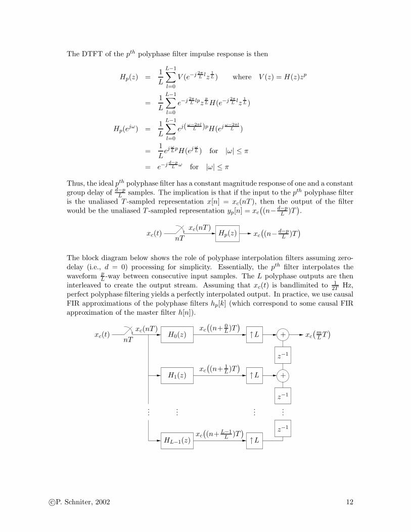
The block diagram below shows the role of polyphase interpolation filters assuming zero-delay (i.e., d = 0) processing for simplicity. Essentially, the pth filter interpolates thewaveform p

L -way between consecutive input samples. The L polyphase outputs are theninterleaved to create the output stream. Assuming that xc(t) is bandlimited to 1

2T Hz,perfect polyphase filtering yields a perfectly interpolated output. In practice, we use causalFIR approximations of the polyphase filters hp[k] (which correspond to some causal FIRapproximation of the master filter h[n]).

H0(z)

H1(z)

HL−1(z)

......

......

nTxc(t)

xc(nT ) xc

((n+ 0

L)T)

xc

((n+ 1

L)T)

xc

((n+ L−1

L )T) z−1

z−1

z−1

+

+

↑L

↑L

↑L xc

(mL T)


• Polyphase Resampling with a Rational Factor: Recall that resampling by rational rate LM

can be accomplished through the following three-stage process.


M

DC gain L

If we implemented the upsampler/LPF pair with a polyphase filterbank, we would stillwaste computations due to eventual downsampling by M . Alternatively, if we implementedthe LPF/downsampler pair with a polyphase filterbank, we would waste computations byfeeding it the (mostly-zeros) upsampler output. Thus, we need to examine this problemin more detail.

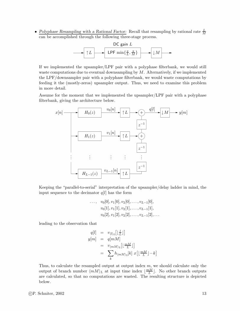
Assume for the moment that we implemented the upsampler/LPF pair with a polyphasefilterbank, giving the architecture below.

x[n] y[m]v0[n]

v1[n]

vL−1[n]

q[l]

+

+

z−1

z−1

z−1

......

......

...

H0(z)

H1(z)

HL−1(z)

↓M

↑L

↑L

↑L

Keeping the “parallel-to-serial” interpretation of the upsampler/delay ladder in mind, theinput sequence to the decimator q[l] has the form

. . . , v0[0], v1[0], v2[0], . . . , vL−1[0],

v0[1], v1[1], v2[1], . . . , vL−1[1],

v0[2], v1[2], v2[2], . . . , vL−1[2], . . .

leading to the observation that

q[l] = v〈l〉L[⌊ l

L⌋]

y[m] = q[mM ]

= v〈mM〉L

[⌊mM

L ⌋]

=∑

k

h〈mM〉L[k] x[⌊mM

L ⌋−k]

Thus, to calculate the resampled output at output index m, we should calculate only theoutput of branch number 〈mM〉L at input time index ⌊mM

L ⌋. No other branch outputsare calculated, so that no computations are wasted. The resulting structure is depictedbelow.


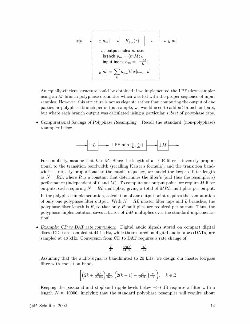
x[n] x[nm] y[m]Hpm(z)

at output index m use:

branch pm = 〈mM〉Linput index nm = ⌊mM

L ⌋.

y[m] =∑

k

hpm[k]x[nm−k]

An equally-efficient structure could be obtained if we implemented the LPF/downsamplerusing an M -branch polyphase decimator which was fed with the proper sequence of inputsamples. However, this structure is not as elegant: rather than computing the output of one

particular polyphase branch per output sample, we would need to add all branch outputs,but where each branch output was calculated using a particular subset of polyphase taps.

• Computational Savings of Polyphase Resampling: Recall the standard (non-polyphase)resampler below.


M

For simplicity, assume that L > M . Since the length of an FIR filter is inversely propor-tional to the transition bandwidth (recalling Kaiser’s formula), and the transition band-width is directly proportional to the cutoff frequency, we model the lowpass filter lengthas N = RL, where R is a constant that determines the filter’s (and thus the resampler’s)performance (independent of L and M). To compute one output point, we require M filteroutputs, each requiring N = RL multiplies, giving a total of MRL multiplies per output.

In the polyphase implementation, calculation of one output point requires the computationof only one polyphase filter output. With N = RL master filter taps and L branches, thepolyphase filter length is R, so that only R multiplies are required per output. Thus, thepolyphase implementation saves a factor of LM multiplies over the standard implementa-tion!

• Example: CD to DAT rate conversion: Digital audio signals stored on compact digitaldiscs (CDs) are sampled at 44.1 kHz, while those stored on digital audio tapes (DATs) aresampled at 48 kHz. Conversion from CD to DAT requires a rate change of

LM = 48000

44100 = 160147

Assuming that the audio signal is bandlimited to 20 kHz, we design our master lowpassfilter with transition bands

[(

2k + 2022.05

)π

160 ,(

2(k + 1) − 2022.05

)π

160

)

, k ∈ Z

Keeping the passband and stopband ripple levels below −96 dB requires a filter with alength N ≈ 10000, implying that the standard polyphase resampler will require about


NM = 1.5 million multiplications per output, or 70 billion multiplications per second!If the equivalent polyphase implementation is used instead, we require only N/L ≈ 62multiplies per output, or 3 million multiplications per second.

• Polyphase Resampling with Arbitrary (Non-Rational or Time-Varying) Rate: Though we

have derived a computationally efficient polyphase resampler for rational factors Q = LM ,

the structure will not be practical to implement for large L, such as might occur whenthe desired resampling factor Q is not well approximated by a ratio of two small integers.Furthermore, we may encounter applications in which Q is chosen on-the-fly, so thatthe number L of polyphase branches cannot be chosen a priori. Fortunately, a slightmodification of our existing structure will allow us to handle both of these cases.

Say that our goal is to produce the QT -rate samples xc(m

TQ) given the 1

T -rate samples

xc(nT ), where we assume that xc(t) is bandlimited to 12T and Q can be any positive real

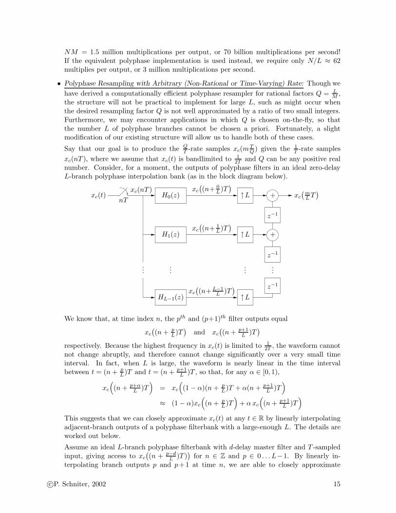
number. Consider, for a moment, the outputs of polyphase filters in an ideal zero-delayL-branch polyphase interpolation bank (as in the block diagram below).

H0(z)

H1(z)

HL−1(z)

......

......

nTxc(t)

xc(nT ) xc

((n+ 0

L)T)

xc

((n+ 1

L)T)

xc

((n+ L−1

L )T) z−1

z−1

z−1

+

+

↑L

↑L

↑L xc

(mL T)

We know that, at time index n, the pth and (p+1)th filter outputs equal

xc

((n + p

L)T)

and xc

((n + p+1

L )T)

respectively. Because the highest frequency in xc(t) is limited to 12T , the waveform cannot

not change abruptly, and therefore cannot change significantly over a very small timeinterval. In fact, when L is large, the waveform is nearly linear in the time intervalbetween t = (n + p

L)T and t = (n + p+1L )T , so that, for any α ∈ [0, 1),

xc

(

(n + p+αL )T

)

= xc

(

(1 − α)(n + pL)T + α(n + p+1

L )T)

≈ (1 − α)xc

(

(n + pL)T

)

+ α xc

(

(n + p+1L )T

)

This suggests that we can closely approximate xc(t) at any t ∈ R by linearly interpolatingadjacent-branch outputs of a polyphase filterbank with a large-enough L. The details areworked out below.

Assume an ideal L-branch polyphase filterbank with d-delay master filter and T -sampledinput, giving access to xc

((n + p−d

L )T ))

for n ∈ Z and p ∈ 0 . . . L−1. By linearly in-terpolating branch outputs p and p+1 at time n, we are able to closely approximate


xc

((n + p−d+α

L )T ))

for any α ∈ [0, 1). We would like to approximate y[m] = xc(mTQ − dT

L )in this manner—note the inclusion of the master filter delay. So, for a particular m, Q, d,and L, we would like to find n ∈ Z, p ∈ 0 . . . L−1, and α ∈ [0, 1) such that

(

n +p − d + α

L

)

T = mT

Q− d

T

L

nL + p + α =mL

Q

=

(m

Q

)

L

=

(⌊m

Q

⌋

+

⟨m

Q

⟩

1

)

L

=

⌊m

Q

⌋

L +

⌊⟨m

Q

⟩

1

L

⌋

+

⟨⟨m

Q

⟩

1

L

⟩

1

=

⌊m

Q

⌋

︸︷︷︸

∈ Z

L +

⌊⟨m

Q

⟩

1

L

⌋

︸︷︷︸

∈ 0 . . . L − 1

+

⟨mL

Q

⟩

1︸︷︷︸

∈ [0, 1)

Thus, we have found suitable n, p, and α. Making clear the dependence on output timeindex m, we write

nm =

⌊m

Q

⌋

pm =

⌊⟨m

Q

⟩

1

L

⌋

αm =

⟨mL

Q

⟩

1

and generate output y[m] ≈ xc(mTQ − dT

L ) via

y[m] = (1−αm)∑

k

hpm[k]x[nm−k] + αm

∑

k

hpm+1[k]x[nm−k]

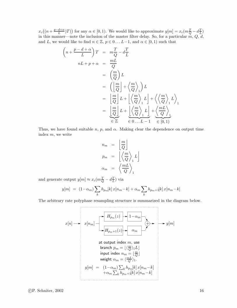
The arbitrary rate polyphase resampling structure is summarized in the diagram below.

x[n] x[nm] y[m]+

1−αmHpm(z)

αmHpm+1(z)

at output index m, use

branch pm = ⌊〈mQ 〉1L⌋

input index nm = ⌊mQ ⌋

weight αm = 〈mLQ 〉1.

y[m] = (1−αm)∑

k hpm[k]x[nm−k]+αm

∑

k hpm+1[k]x[nm−k]


Note that our structure refers to polyphase filters Hpm(z) and Hpm+1(z) for pm ∈ 0 . . . L−1.This specifies the standard polyphase bank H0(z), . . . ,HL−1(z) plus the additional filterHL(z). Ideally the pth filter has group delay d−p

L , so that HL(z) should advance the inputone full sample relative to H0(z), i.e., HL(z) = zH0(z). There are a number of ways todesign/implement the additional filter.

1. Design a master filter of length LR + 1 (where R is the polyphase filter length), andthen construct

hp[k] = h[kL + p] for p ∈ 0 . . . L.

Note that hL[k] = h0[k + 1] for 0 ≤ k ≤ R − 2.

2. Set HL(z) = H0(z) and advance the input stream to the last filter by one sample(relative to the other filters).

In certain applications the rate of resampling needs to be adjusted on-the-fly. The arbitraryrate resampler easily facilitates this requirement by replacing Q with Qm in the definitionsfor nm, pm, and αm.

Polyphase filter design follows either an indirect approach, where a master filter with DCgain L and cutoff frequency min π

L , QπL is designed and later split into polyphase filters,

or a direct approach, where each filter is independantly designed to approximate an idealfractional-delay filter. For the direct approach, we require that Q ≥ 1 (or Q ≈ 1) sincethe otherwise the filterbank would not perform the necessary anti-aliasing function.

Finally, it should be emphasized that L, the number of branches, must be chosen largeenough so that the errors due to linear interpolation are negligible. (As such, it is nota function of Q.) If we instead use a more sophisticated interpolation method, e.g., La-grange interpolation involving more than two branch outputs, then fewer polyphase filterswould be necessary for the same overall performance, reducing the storage requirementsfor polyphase filter taps. On the other hand, combining the outputs of more branchesrequires more computations per output point. In the end, we have a tradeoff betweenstorage and computation.

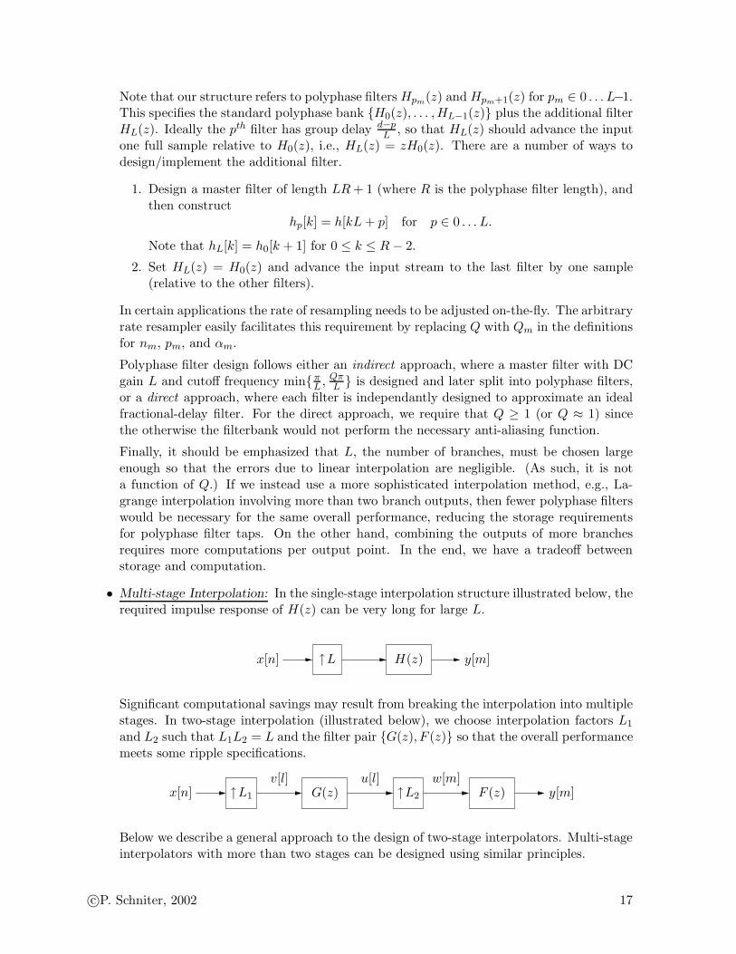
• Multi-stage Interpolation: In the single-stage interpolation structure illustrated below, therequired impulse response of H(z) can be very long for large L.

x[n] y[m]↑L H(z)

Significant computational savings may result from breaking the interpolation into multiplestages. In two-stage interpolation (illustrated below), we choose interpolation factors L1

and L2 such that L1L2 = L and the filter pair G(z), F (z) so that the overall performancemeets some ripple specifications.

x[n]v[l] u[l] w[m]

y[m]↑L1 ↑L2 F (z)G(z)

Below we describe a general approach to the design of two-stage interpolators. Multi-stageinterpolators with more than two stages can be designed using similar principles.


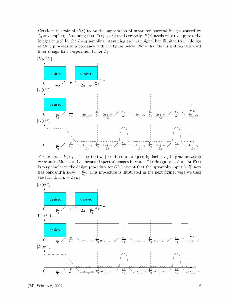
Consider the role of G(z) to be the suppression of unwanted spectral images caused byL1-upsampling. Assuming that G(z) is designed correctly, F (z) needs only to suppress theimages caused by the L2-upsampling. Assuming an input signal bandlimited to ω0, designof G(z) proceeds in accordance with the figure below. Note that this is a straightforwardfilter design for interpolation factor L1.

|X(ejω)|

|V (ejω)|

|G(ejω)|

ω

ω

ω0

0

0

π 2π2π−ω0ω0

ω0

L1

ω0

L1

πL1

πL1

2π−ω0

L1

2π−ω0

L1

2πL1

2πL1

2π+ω0

L1

2π+ω0

L1

3πL1

3πL1

4π−ω0

L1

4π−ω0

L1

4πL1

4πL1

4π+ω0

L1

4π+ω0

L1

5πL1

5πL1

6π−ω0

L1

6π−ω0

L1

desired

desireddesired

. . .

. . .

For design of F (z), consider that u[l] has been upsampled by factor L2 to produce w[m];we want to filter out the unwanted spectral images in w[m]. The design procedure for F (z)is very similar to the design procedure for G(z) except that the upsampler input (u[l]) nowhas bandwidth L2

ω0

L = ω0

L1. This procedure is illustrated in the next figure, were we used

the fact that L = L1L2.

|U(ejω)|

|W (ejω)|

|F (ejω)|

ω

ω

ω0

0

0

π 2π2π− ω0

L1

ω0

L1

ω0

L

ω0

L

πL2

πL2 2πL1−ω0

L

2πL1−ω0

L

2πL2

2πL2

2πL1+ω0

L

2πL1+ω0

L

3πL2

3πL2

4πL1−ω0

L

4πL1−ω0

L

4πL2

4πL2

4πL1+ω0

L

4πL1+ω0

L

5πL2

5πL2

6πL1−ω0

L

6πL1−ω0

L

desired

desireddesired

. . .

. . .


We now address the ripple specifications on F (z) and G(z) relative to those on H(z).Because ripple from the passbands of G(z) and F (z) could add constructively, we set thepassband ripple requirements for each filter equal to half of the total allowable passbandripple δp, i.e., that of H(z). It is sufficient to set the stopband ripple requirements for eachfilter equal to the total allowable stopband ripple δs, i.e., that of H(z), if we assume thatthe none of the transition-band gains exceed the passband gain.

In multi-stage interpolation, it is common to choose a small value for L1 (e.g., L1 = 2).This choice will become more clear later, when we consider the computational savings ofmulti-stage interpolation.

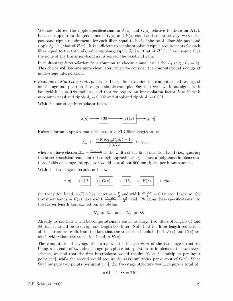
• Example of Multi-stage Interpolation: Let us first examine the computational savings ofmulti-stage interpolation through a simple example. Say that we have input signal withbandwidth ω0 = 0.9π radians, and that we require an interpolation factor L = 30 withmaximum passband ripple δp = 0.002 and stopband ripple δs = 0.001.

With the one-stage interpolator below,

x[n] y[m]↑30 H(z)

Kaiser’s formula approximates the required FIR filter length to be

Nh ≈−10 log10(δpδs) − 13

2.3∆ω≈ 900,

where we have chosen ∆ω = 2π−2ω0

L as the width of the first transition band (i.e., ignoringthe other transition bands for this rough approximation). Thus, a polyphase implementa-tion of this one-stage interpolator would cost about 900 multiplies per input sample.

With the two-stage interpolator below,

x[n] y[m]↑2 ↑15 F (z)G(z)

the transition band in G(z) has center ω = π2 and width 2π−2ω0

2 = 0.1π rad. Likewise, thetransition bands in F (z) have width 4π−2ω0

30 = 2.230 π rad. Plugging these specifications into

the Kaiser length approximation, we obtain

Ng ≈ 64 and Nf ≈ 88.

Already we see that it will be computationally easier to design two filters of lengths 64 and88 than it would be to design one length-900 filter. Note that the filter-length reductionsof this structure result from the fact that the transition bands in both F (z) and G(z) aremuch wider than the transition band in H(z).

The computational savings also carry over to the operation of the two-stage structure.Using a cascade of two single-stage polyphase interpolators to implement the two-stagescheme, we find that the first interpolator would require Ng ≈ 64 multiplies per inputpoint x[n], while the second would require Nf ≈ 88 multiplies per output of G(z). SinceG(z) outputs two points per input x[n], the two-stage structure would require a total of

≈ 64 + 2 · 88 = 240


multiplies per input x[n]. Clearly this is a significant savings over the 900 multipliesrequired by the one-stage polyphase structure. Note that it was advantageous to choosethe first upsampling ratio (L1) as a small number, else the second stage of interpolationwould need to operate at higher rate and the total number of multiplications per input

point x[n] would increase.

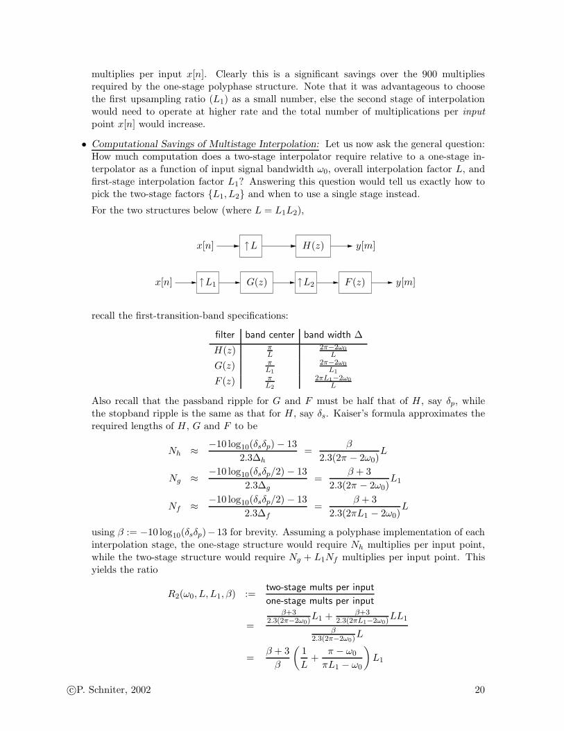
• Computational Savings of Multistage Interpolation: Let us now ask the general question:How much computation does a two-stage interpolator require relative to a one-stage in-terpolator as a function of input signal bandwidth ω0, overall interpolation factor L, andfirst-stage interpolation factor L1? Answering this question would tell us exactly how topick the two-stage factors L1, L2 and when to use a single stage instead.

For the two structures below (where L = L1L2),

x[n] y[m]↑L H(z)

x[n] y[m]↑L1 ↑L2 F (z)G(z)

recall the first-transition-band specifications:

filter band center band width ∆

H(z) πL

2π−2ω0

L

G(z) πL1

2π−2ω0

L1

F (z) πL2

2πL1−2ω0

L

Also recall that the passband ripple for G and F must be half that of H, say δp, whilethe stopband ripple is the same as that for H, say δs. Kaiser’s formula approximates therequired lengths of H, G and F to be

Nh ≈−10 log10(δsδp) − 13

2.3∆h=

β

2.3(2π − 2ω0)L

Ng ≈−10 log10(δsδp/2) − 13

2.3∆g=

β + 3

2.3(2π − 2ω0)L1

Nf ≈−10 log10(δsδp/2) − 13

2.3∆f=

β + 3

2.3(2πL1 − 2ω0)L

using β := −10 log10(δsδp)− 13 for brevity. Assuming a polyphase implementation of eachinterpolation stage, the one-stage structure would require Nh multiplies per input point,while the two-stage structure would require Ng + L1Nf multiplies per input point. Thisyields the ratio

R2(ω0, L, L1, β) :=two-stage mults per input

one-stage mults per input

=

β+32.3(2π−2ω0)L1 + β+3

2.3(2πL1−2ω0)LL1

β2.3(2π−2ω0)L

=β + 3

β

(1

L+

π − ω0

πL1 − ω0

)

L1


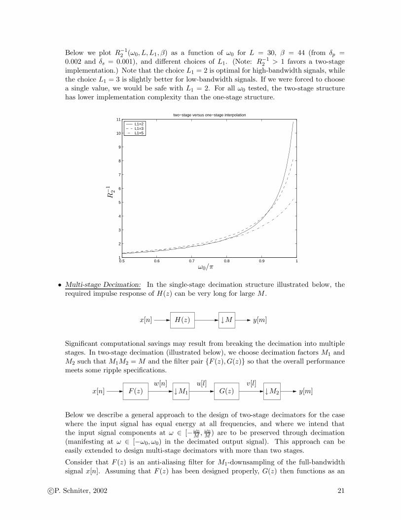
Below we plot R−12 (ω0, L, L1, β) as a function of ω0 for L = 30, β = 44 (from δp =

0.002 and δs = 0.001), and different choices of L1. (Note: R−12 > 1 favors a two-stage

implementation.) Note that the choice L1 = 2 is optimal for high-bandwidth signals, whilethe choice L1 = 3 is slightly better for low-bandwidth signals. If we were forced to choosea single value, we would be safe with L1 = 2. For all ω0 tested, the two-stage structurehas lower implementation complexity than the one-stage structure.

0.5 0.6 0.7 0.8 0.9 11

2

3

4

5

6

7

8

9

10

11two−stage versus one−stage interpolation

L1=2L1=3L1=5

R−

12

ω0/π

• Multi-stage Decimation: In the single-stage decimation structure illustrated below, therequired impulse response of H(z) can be very long for large M .

x[n] y[m]↓MH(z)

Significant computational savings may result from breaking the decimation into multiplestages. In two-stage decimation (illustrated below), we choose decimation factors M1 andM2 such that M1M2 = M and the filter pair F (z), G(z) so that the overall performancemeets some ripple specifications.

x[n]v[l]u[l]w[n]

y[m]↓M1 ↓M2F (z) G(z)

Below we describe a general approach to the design of two-stage decimators for the casewhere the input signal has equal energy at all frequencies, and where we intend thatthe input signal components at ω ∈ [−ω0

M , ω0

M ) are to be preserved through decimation(manifesting at ω ∈ [−ω0, ω0) in the decimated output signal). This approach can beeasily extended to design multi-stage decimators with more than two stages.

Consider that F (z) is an anti-aliasing filter for M1-downsampling of the full-bandwidthsignal x[n]. Assuming that F (z) has been designed properly, G(z) then functions as an


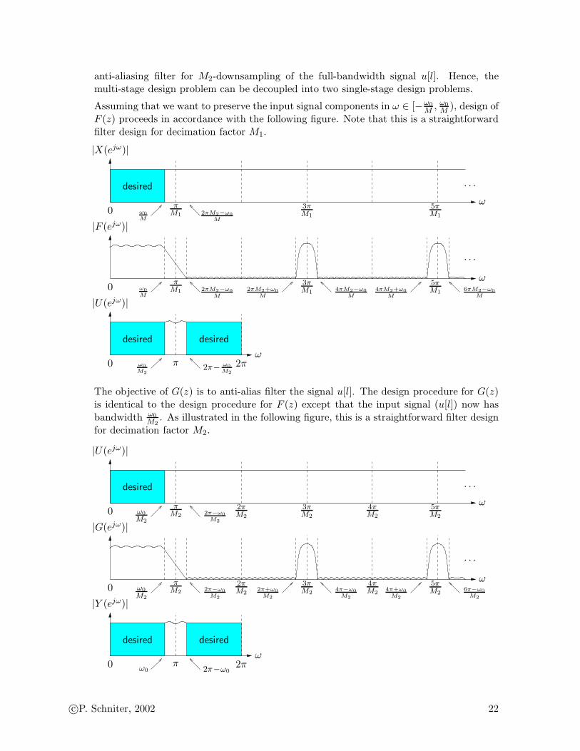
anti-aliasing filter for M2-downsampling of the full-bandwidth signal u[l]. Hence, themulti-stage design problem can be decoupled into two single-stage design problems.

Assuming that we want to preserve the input signal components in ω ∈ [−ω0

M , ω0

M ), design ofF (z) proceeds in accordance with the following figure. Note that this is a straightforwardfilter design for decimation factor M1.

|X(ejω)|

|U(ejω)|

|F (ejω)|

ω

ω

ω0

0

0

ω0

M2

π2π−

ω0

M2

2π

ω0

M

ω0

M

πM1

πM1

2πM2−ω0

M

2πM2−ω0

M

2πM2+ω0

M

3πM1

3πM1

4πM2−ω0

M

4πM2+ω0

M

5πM1

5πM1

6πM2−ω0

M

desireddesired

desired

. . .

. . .

The objective of G(z) is to anti-alias filter the signal u[l]. The design procedure for G(z)is identical to the design procedure for F (z) except that the input signal (u[l]) now hasbandwidth ω0

M2. As illustrated in the following figure, this is a straightforward filter design

for decimation factor M2.

|U(ejω)|

|Y (ejω)|

|G(ejω)|

ω

ω

ω0

0

0

ω0π

2π−ω02π

ω0

M2

ω0

M2

πM2

πM2

2π−ω0

M2

2π−ω0

M2

2πM2

2πM2

2π+ω0

M2

3πM2

3πM2

4π−ω0

M2

4πM2

4πM2

4π+ω0

M2

5πM2

5πM2

6π−ω0

M2

desireddesired

desired

. . .

. . .


We now address the ripple specifications on F (z) and G(z). Recall that, after the firstdecimation stage, the input signal components at frequency ω ∈ [−ω0

M , ω0

M ) will be corruptedby worst-case ripples of

1

M1

(δf,p + (M1 − 1)δf,s

),

where δf,p and δf,s denote the passband and stopband ripples of F (z). Since this spectralregion will occupy the passband of G(z), the first-stage output ripples will, in the worstcase, (approximately) add to the passband ripples of G(z). If we assume that the signalcomponents within the stopband of G(z) have equal energy as the signal components in thepassband, then after two stages of decimation, the input signal components at frequenciesω ∈ [−ω0

M , ω0

M ) will be corrupted by worst-case ripples of

1

M2

(1

M1

(δf,p + (M1 − 1)δf,s

)+ δg,p + (M2 − 1)δg,s

)

≈δf,p

M+

δf,s + δg,p

M2+

(M2 − 1)δg,s

M2,

where the approximation holds when M1 ≫ 1, and where δg,p and δg,s denote the passbandand stopband ripples of G(z). The previous expression suggests that the ripples in G(z)have a greater effect than those in F (z), and that stopband ripples have a greater effectthan passband ripples.

In multi-stage decimation, it is common to choose a small value for M2 (e.g., M2 = 2)since, by putting the bulk of the decimation in the first stage, the second stage can operateat a very low rate. As with the case of interpolation, one could analyze the computationalsavings precisely for various choices of M2.


Multirate notes

Documents

Transcript of Multirate notes