MANUEL M. MATHEWII MA ECONOMICSUNIVERSITY COLLEGE TRIVANDRUM

relates business cycles to the internal

workings of the economy, showing how

changes in investment and output reinforce

each other; the central ingredients of the

model are the multiplier and accelerator.

Samuelson’s Model of Business Cycles:

Interaction between Multiplier and Accelerator

Multiplier is the factor by which a change

in a component of agg.dd,like C or I or G is

multiplied to lead to a larger change in

equilibrium national output. The multiplier

principle is so named because relatively small

autonomous changes generate relatively

larger, or multiple, induced changes in

agg.production.This principle is commonly

represented by a multiplier, which is a specific

number with a value greater than 1.

Accelerator is the relation between

change in I due to a change in Y. Kt = v.Yt

where Kt is the stock of capital at time period

t, v is the capital - output ratio (assumed to be

constant) and Yt is the income in time period

t. Under the assumption that v is constant, we

can also write ∆K = v. ∆Y or v is the

accelerator.

An autonomous increase in the level of

investment raises income by a

magnified amount depending upon the

value of the multiplier.

This increase in income further induces

the increase in investment through the

acceleration effect.

Combining Accelerator with

Keynesian Multiplier

Where ∆Ia = Increase in Autonomous

Investment

∆Y=Increase in Income.

1/ 1 – MPC = Size of Multiplier where

MPC = Marginal Propensity to

Consume.

∆ld = Increase in Induced Investment

v = Size of accelerator.

Mathematical

Representation Yt = Ct + It …(i)

Ct= Ca + c (Yt – 1) …(ii)

It = Ia + v (Y t – 1 – Y t – 2)….(iii)

Yt ,Ct ,It =income, consumption and

investment respectively for a period t,

Ca=autonomous consumption

la =autonomous investment,

c =marginal propensity to consume

v= capital-output ratio or accelerator.

Substituting equations (ii) and

(iii) in equation (i)

Yt = Ca + c (Yt - 1) + Ia + v (Y t – 1 – Y t – 2) …(iv)

Equation (iv) describes the path which a

disequilibrium system follows to reach either a

final equilibrium state or moves away from it. But

whether the economy moves towards a new

equilibrium or deviates away from it depends on

the values of marginal propensity to consume (c)

and capital-output ratio v (i.e., accelerator).

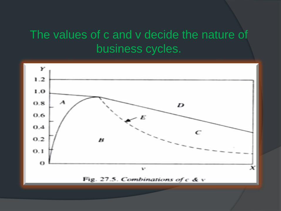
The values of c and v decide the nature of

business cycles.

When the combinations of the value of marginal

propensity to consume (c) and capital-output

ratio (v) lie within the region marked A, with a

change in autonomous investment, the gross

national product or income moves upward or

downward at a decreasing rate and finally

reaches a new equilibrium

If the values of c and v are such that they lie

within the region B, the change in autonomous

investment or autonomous consumption will

generate fluctuations in income which follow

the pattern of a series of damped cycles whose

amplitudes go on declining until the cycles

disappear

The region C represents the combinations of c and v

which are relatively high as compared to the region

B and determine such values of multiplier and

accelerator that bring about explosive cycles, that is,

the fluctuations of income with successively greater

and greater amplitude.

Panel c shows that the system tends to explode and

diverges greatly from the equilibrium level.

The region D provides the combinations of c and v

which cause income to move upward or downward at

an increasing rate which has somehow to be

restrained if the cyclical movements are to occur.

This is depicted in panel (d). Like the values of

multiplier and accelerator of region C, their values in

region D cause the system to explode and diverge

from the equilibrium state by an increasing amount.

In a special case when values of c and v (and

therefore the magnitudes of multiplier and

accelerator) lie in region E, they produce

fluctuations in income of constant amplitude

as is shown in panel (e).

Only combinations B, C and E produce

business cycles. The upper limit is the

buffer imposed by real life constraints

beyond which cycles can't explode.

One of the famous theories of business

cycles based on the interaction of

multiplier and accelerator was put forward

by the English economist J.R. Hicks.

Assume that marginal propensity to consume (c) =2/3 or 0.66

capital-output ratio (v) or accelerator being equal = 2.

Period up to t + 6 represents the expansion phase or upswing of the

business cycle.

t + 13 represents the lower turning point of the business cycle.

Beyond the period t + 13, income again starts rising that is, recovery

from the depression begins.

Limitations

THANK YOU……