Multiplicative weights method: A meta algorithm with applications
31
Multiplicative weights method: A meta algorithm with applications to linear and semi-definite programming Sanjeev Arora Princeton University Based upon: Fast algorithms for Approximate SDP [FOCS ‘05] √log(n) approximation to SPARSEST CUT in Õ(n 2 ) time [FOCS ‘04] The multiplicative weights update method and it’s applications [’05] See also recent papers by Hazan and Kale.
Transcript of Multiplicative weights method: A meta algorithm with applications

Multiplicative weights method: A meta algorithm with applications to linear
and semidefinite programming
Sanjeev AroraPrinceton University
Based upon:Fast algorithms for Approximate SDP [FOCS ‘05]√log(n) approximation to SPARSEST CUT in Õ(n2) time [FOCS ‘04]The multiplicative weights update method and it’s applications [’05]See also recent papers by Hazan and Kale.

Multiplicative update rule (long history)
Applications: approximate solutions to LPs and SDPs, flow problems,
online learning (boosting), derandomization & chernoff bounds,
online convex optimization, computational geometry,
metricembeddongs, portfolio management… (see our survey)
w1
w2
.
.
.
wn
n agents weights
Update weights according toperformance:
wit+1 Ã wi
t (1 + ε ¢ performance of i)
Simplest setting – predicting the market
N “experts” on TV
Can we perform as good as the best expert ?
1$ for correct prediction
0$ for incorrect

Weighted majority algorithm [LW ‘94]
Multiplicative update (initially all wi =1):
If expert predicted correctly: wit+1 Ã wi
t
If incorrectly, wit+1 Ã wi
t(1 ε)
Claim: #mistakes by algorithm ¼ 2(1+ε)(#mistakes by best expert)Potential: φt = Sum of weights= ∑i wi
t (initially n)
If algorithm predicts incorrectly ) φt+1 · φt ε φt /2
φT · (1ε/2)m(A) n m(A) =# mistakes by algorithm
φT ¸ (1ε)mi
) m(A) · 2(1+ε)mi + O(log n/ε)
“Predict according to the weighted majority.”

Generalized Weighted majority [A.,Hazan, Kale ‘05]
n agents Set of events (possibly infinite)
event j
expert ipayoffM(i,j)
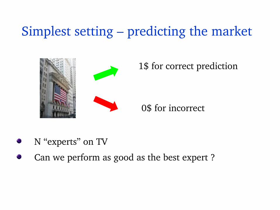
Generalized Weighted majority [AHK ‘05]
n agents Set of events (possibly infinite)
Claim: After T iterations,
Algorithm payoff ¸ (1ε) best expert – O(log n / ε)
Algorithm: plays distribution on experts (p1,…,pn)
Payoff for event j: ∑i pi M(i,j)
Update rule:pi
t+1 Ã pit (1 + ε ¢ M(i,j))
p1
p2
.
.
.
pn

Game playing,Online optimization
Lagrangean relaxation
Gradient descent
Chernoff bounds
Games with Matrix Payoffs Fast soln to
LPs, SDPs
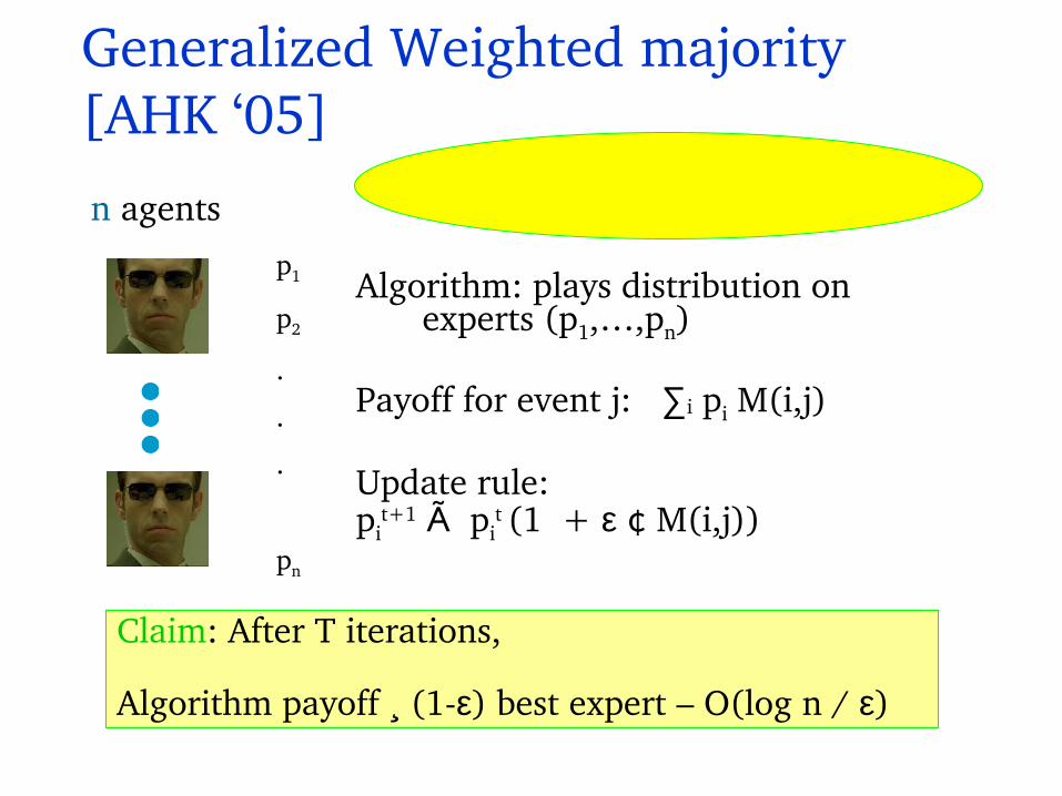
Common features of MW algorithms
“competition” amongst n experts
Appearance of terms like
exp( ∑t (performance at time t) )
Time to get εapproximate solutions is proportional to 1/ε2.

Application1 : Approximate solutions to LPs (“Combinatorial”)
Plotkin Shmoys Tardos ’91Young’97Garg Koenemann’99Fleischer’99
MW MetaAlgorithm gives unified view
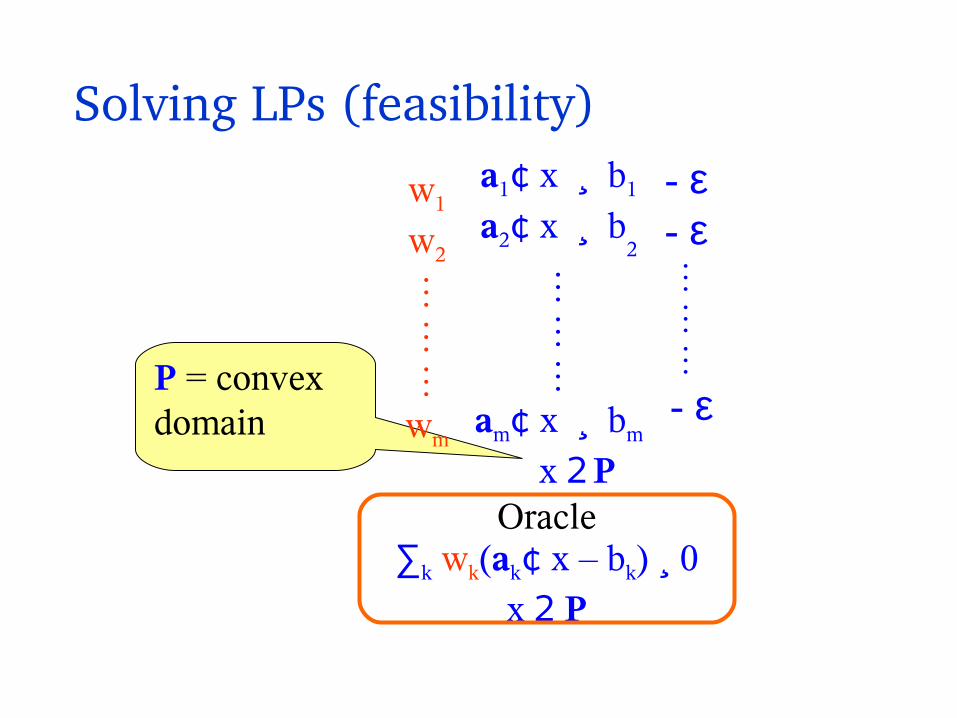
Solving LPs (feasibility)a1¢ x ¸ b1
a2¢ x ¸ b2
am¢ x ¸ bm
x 2 P
∑k wk(ak¢ x – bk) ¸ 0x 2 P
P = convex domain
- ε- ε
- ε
w1
w2
wm
Oracle
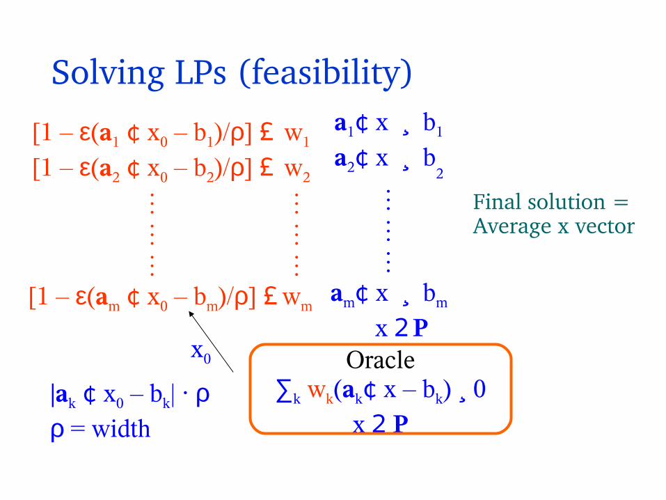
Solving LPs (feasibility)a1¢ x ¸ b1
a2¢ x ¸ b2
am¢ x ¸ bm
x 2 P
w1
w2
wm
[1 – ε(a1 ¢ x0 – b1)/ρ] £[1 – ε(a2 ¢ x0 – b2)/ρ] £
[1 – ε(am ¢ x0 – bm)/ρ] £
x0
|ak ¢ x0 – bk| · ρρ = width
∑k wk(ak¢ x – bk) ¸ 0x 2 P
Oracle
Final solution =Average x vector

Performance guarantees
In O(ρ2 log(n)/ε2) iterations, average x is ε feasible.
PackingCovering LPs: [Plotkin, Shmoys, Tardos ’91]
9? x 2 P:
j = 1, 2, … m: aj ¢ x ¸ 1
Want to find x 2 P s.t. aj ¢ x ¸ 1 ε
Assume: 8 x 2 P: 0 · aj ¢ x · ρ
MW algorithm gets ε feasible x in O(ρ log(n)/ε2)
iterations
Covering problem

Connection to Chernoff bounds and derandomizationDeterministic approximation algorithms for 0/1 packing/covering problem a la RaghavanThompson
Solve LP relaxation of integer program.Obtain soln (yi)
Randomized Rounding O(log n) times)
xi à 1 w/ prob. yi
xi à 0 w/ prob.1 yi
Derandomize using pessimistic estimators
exp(∑i t ¢ f(yi))Young [95] “Randomized rounding without solving the LP.” MW update rule mimics pessimistic estimator.
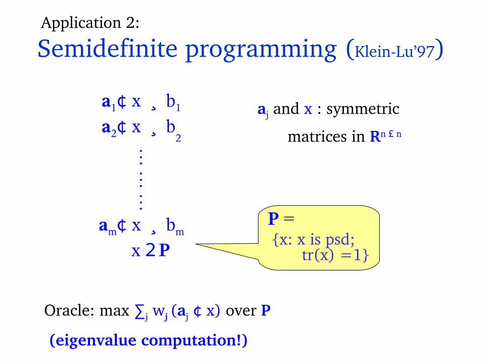
Semidefinite programming (KleinLu’97)
a1¢ x ¸ b1
a2¢ x ¸ b2
am¢ x ¸ bm
x 2 P
P =
aj and x : symmetric
matrices in Rn £ n
{x: x is psd; tr(x) =1}
Oracle: max ∑j wj (aj ¢ x) over P
(eigenvalue computation!)
Application 2:

Next few slides: New Results (AHK’04, AHK’05)
Key difference between efficient and notsoefficient implementations of the MW idea: Width management.
(e.g., the difference between PST’91 and GK’99)

Solving SDP relaxations more efficiently [AHK’05]
Õ(n3/ε2)Õ(n4.5)SPARSEST CUT
Õ(n3.5/ε2)Õ(n4.5)MIN UNCUT etc
Õ(n1.5N/ε4.5)Õ(n4)SCP
Õ(n3/d5ε3.5)Õ(n4)EMBEDDING
Õ(n2.5/ε2.5)Õ(n4)HAPLOFREQ
Õ(n1.5N/ε2.5) or
Õ(n3/α*ε3.5)
Õ(n3.5)MAXQP (e.g. MAXCUT)
Our resultUsing Interior PointProblem

Recall: issue of width
Õ(ρ2/ε2) iterations to
obtain ε feasible x
ρ = maxk |ak ¢ x –
bk|
ρ is too large!!
MWa1¢ x ¸ b1
a2¢ x ¸ b2
am¢ x ¸ bm
Oracle
∑k wk(ak¢ x – bk) ¸ 0x 2 P

Issue 1:Dealing with width
A few high width
constraints
Oracle: separation
hyperplane for dual
Can run
ellipsoid/Vaidya
poly(m, log(ρ/ε))
iterations to obtain ε
feasible x
MWa1¢ x ¸ b1
a2¢ x ¸ b2
am¢ x ¸ bm
Oracle
∑k wk(ak¢ x – bk) ¸ 0x 2 P
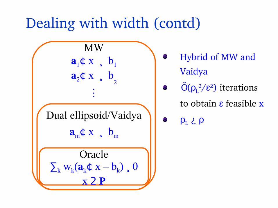
Hybrid of MW and
Vaidya
Õ(ρL2/ε2) iterations
to obtain ε feasible x
ρL ¿ ρ
MWa1¢ x ¸ b1
a2¢ x ¸ b2
am¢ x ¸ bm
Oracle
∑k wk(ak¢ x – bk) ¸ 0x 2 P
Dual ellipsoid/Vaidya
Dealing with width (contd)
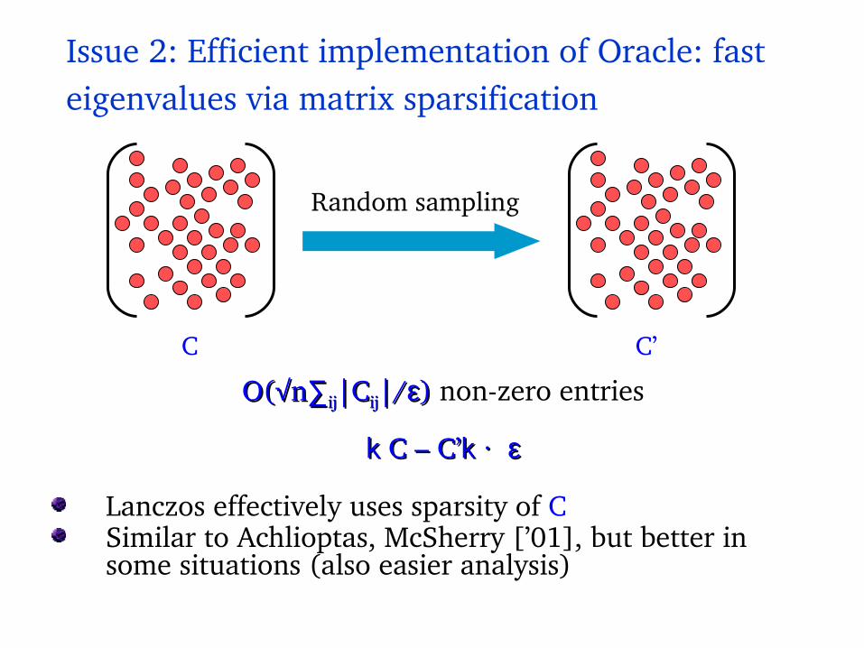
Issue 2: Efficient implementation of Oracle: fast eigenvalues via matrix sparsification
Lanczos effectively uses sparsity of CSimilar to Achlioptas, McSherry [’01], but better in some situations (also easier analysis)
C
O(O(√√nn∑∑ijij|C|Cijij|/|/εε)) nonzero entries
k k C – C’C – C’k ·k · εε
Random sampling
C’

Online games with matrix payoffs(Satyen Kale’06)
Payoff is a matrix, and so is the “distribution” on experts!
Uses matrix analogues of usual inequalities
1+ x · ex I + A · eA
Used (together with many other tricks) to solve “triangleinequality” SDPs in O(n3) time.
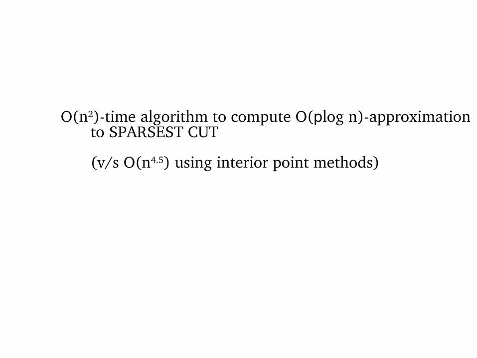
O(n2)time algorithm to compute O(plog n)approximationto SPARSEST CUT
(v/s O(n4.5) using interior point methods)

Sparsest Cut
S
O(log n) approximation [Leighton Rao ’88]
O(plog n) approximation [A., Rao, Vazirani’04]
O(p log n) approximation in O(n2) time. (Actually, finds expander flows) [A., Hazan, Kale’05]
The sparsest cut:
® := minS µ V ; jS j< V =2
jE (S; ¹S)jjSj
Sα(G) = 2/5

MW algorithm to find expander flows
Events – { (s,w,z) | weights on vertices, edges, cuts}
Experts – pairs of vertices (i,j)
Payoff: (for weights di,j on experts)
Fact: If events are chosen optimally, the distribution on experts di,j
converges to a demand graph which is an “expander flow”
[by results of AroraRaoVazirani ’04 suffices to produce approx.
sparsest cut]
Pi j di j (si + sj + l i j ¡ zi j )
shortest path according to weights we
Cuts separating i and j
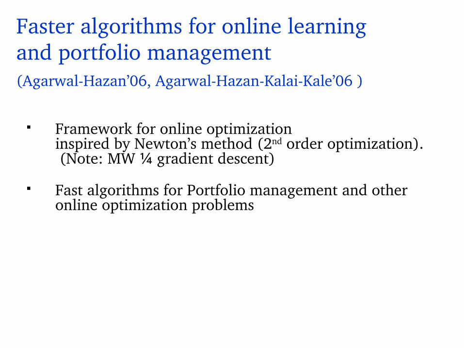
Faster algorithms for online learningand portfolio management (AgarwalHazan’06, AgarwalHazanKalaiKale’06 )
Framework for online optimization inspired by Newton’s method (2nd order optimization). (Note: MW ¼ gradient descent)
Fast algorithms for Portfolio management and other online optimization problems

Open problems
Better approaches to width management?
Faster run times?
THANK YOU

Connection to Chernoff bounds and derandomization
Deterministic approximation algorithms a la RaghavanThompson
Packing/covering IP with variables xi = 0/1
9? x 2 P: 8 j 2 [m], fj(x) ¸ 0
Solve LP relaxation using variables yi 2 [0, 1]
Randomized rounding:
xi =
Chernoff: O(log m) sampling iterations suffice
1 w.p. yi
0 w.p. 1 – yi
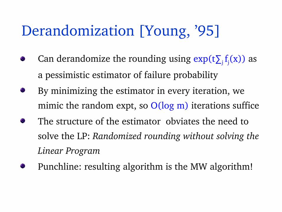
Derandomization [Young, ’95]
Can derandomize the rounding using exp(t∑j fj(x)) as
a pessimistic estimator of failure probability
By minimizing the estimator in every iteration, we
mimic the random expt, so O(log m) iterations suffice
The structure of the estimator obviates the need to
solve the LP: Randomized rounding without solving the
Linear Program
Punchline: resulting algorithm is the MW algorithm!

Weighted majority [LW ‘94]
If lost at t, φt+1 · (1½ ε) φt
At time T: φT · (1½ ε)#mistakes ¢ φ0
Overall:
#mistakes · log(n)/ε + (1+ε) mi
#mistakes ofexpert i
(1 ¡ " )m i = wTi ·
X
i
wTi = ©T
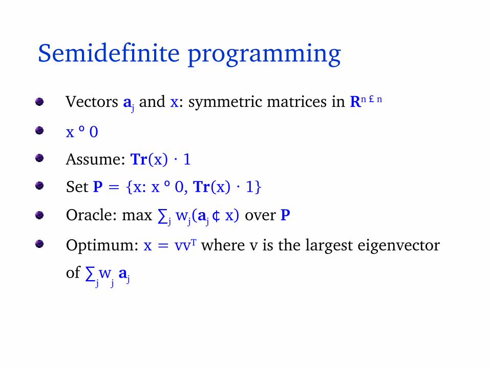
Semidefinite programming
Vectors aj and x: symmetric matrices in Rn £ n
x º 0
Assume: Tr(x) · 1
Set P = {x: x º 0, Tr(x) · 1}
Oracle: max ∑j wj(aj ¢ x) over P
Optimum: x = vvT where v is the largest eigenvector
of ∑jw
j aj
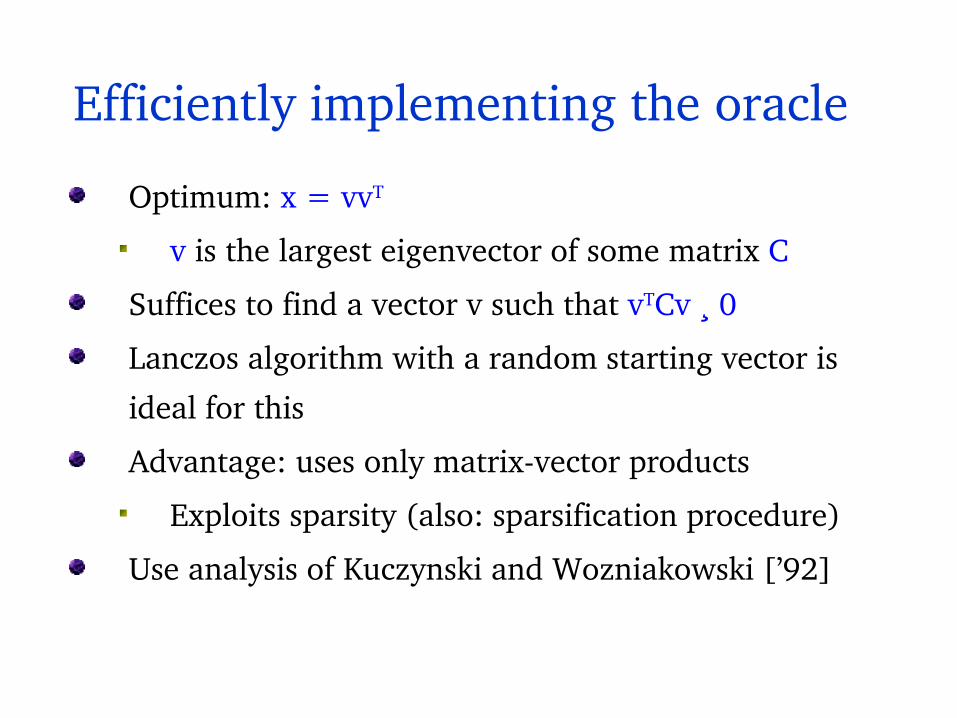
Efficiently implementing the oracle
Optimum: x = vvT
v is the largest eigenvector of some matrix C
Suffices to find a vector v such that vTCv ¸ 0
Lanczos algorithm with a random starting vector is
ideal for this
Advantage: uses only matrixvector products
Exploits sparsity (also: sparsification procedure)
Use analysis of Kuczynski and Wozniakowski [’92]


![QIP = PSPACE · extend this result to all of QIP, establishing the relationship QIP =PSPACE. Similar to [JUW09], we use the matrix multiplicative weights update method, together with](https://static.fdocuments.us/doc/165x107/5f88586338174314853ac9c8/qip-pspace-extend-this-result-to-all-of-qip-establishing-the-relationship-qip.jpg)