Multiple-Vehicle Fire Loads for Precast Concrete Parking ... · This research was funded by in part...

ATLSS is a National Center for Engineering Research on Advanced Technology for Large Structural Systems

117 ATLSS Drive

Bethlehem, PA 18015-4729

Phone: (610)758-3525 www.atlss.lehigh.edu Fax: (610)758-5902 Email: [email protected]

Multiple-Vehicle Fire Loads for Precast Concrete Parking Structures

by

Kyla Strenchock

Stephen Pessiki

ATLSS Report No. 08-03

June 2008

ATLSS is a National Center for Engineering Research on Advanced Technology for Large Structural Systems

117 ATLSS Drive

Bethlehem, PA 18015-4729

Phone: (610)758-3525 www.atlss.lehigh.edu Fax: (610)758-5902 Email: [email protected]

Multiple-Vehicle Fire Loads for Precast Concrete Parking Structures

by

Kyla Strenchock Graduate Research Assistant

Stephen Pessiki

Professor of Structural Engineering [email protected]

ATLSS Report No. 08-03

June 2008

- ii -

ACKNOWLEDGEMENTS

This research was funded by in part by the Precast/Prestressed Concrete Institute. Additional support was provided by Lehigh University. This financial support is gratefully acknowledged. The findings and conclusions included in this report are those of the author and do not necessarily reflect the views of the sponsors.

- iii -

TABLE OF CONTENTS

ABSTRACT 1 1 INTRODUCTION 2 1.1 INTRODUCTION 2 1.2 OBJECTIVE 2 1.3 SUMMARY OF APPROACH 3 1.4 SUMMARY OF FINDINGS 3 1.5 SCOPE OF REPORT 3 1.6 NOTATION 4 1.7 UNIT CONVERSTION FACTORS 4 2 BACKGROUND 5 2.1 REVIEW OF BAYREUTHER (2006) 5 2.2 DESIGN CURVES 6 2.2.1 Time-Temperature Curves 6 2.2.2 Time- Heat Flux Curves 7 2.3 ASTM E 119 END POINT CRITERIA 8 2.4 FIRE MODELING WITH THE FIRE DYNAMICS SIMULATOR 8 3 PROTOTYPE STRUCTURE AND ANALYSIS MATRIX 12 3.1 PROTOTYPE STRUCTURE DESCRIPTION 12 3.2 ANALYSIS MODEL 13 3.2.1 Parking Garage Analysis Model 13 3.2.2 Vehicle Model and Fire Characteristics 13 3.3 FIRE ANALYSES 14 3.3.1 Analysis Matrix 14 3.3.2 Analysis Variable: Vehicle Ignition Time 14 3.3.3 Analysis Variable: Center Wall Opening Position 15 4 FIRE ANALYSIS PROCEDURE 28 4.1 OVERVIEW OF ANALYSIS PROCEDURE 28 4.2 CREATING THE ANALYSIS MODEL 28 4.2.1 Concrete Material Properties 28 4.2.2 Analysis Parameters 29 4.3 RUNNING THE ANALYSIS 30 4.4 FDS OUTPUT DATA 31 5 INDIVIDUAL FIRE ANALYSIS SUMMARIES 36 5.1 FORMAT OF ANALYSIS SUMMARIES 36 5.2 INDIVIDUAL ANALYSIS SUMMARIES 36 5.2.1 12 Min Bottom Analysis 36 5.2.2 6 Min Bottom Analysis 50 5.2.3 6 Min Top Analysis 62 6 DISCUSSION OF FIRE ANALYSIS RESULTS 73 6.1 EFFECTS OF TIME INTERVAL BETWEEN IGNITIONS OF ADJACENT VEHICLES ON HEAT TRANSMISSION 73 6.2 GEOMETRIC EFFECTS ON HEAT TRANSMISSION 74 7 NON-LINEAR HEAT TRANSFER ANALYSIS 81 7.1 NON-LINEAR HEAT TRANSFER ANALYSIS PROCEDURE 81

- iv -

7.1.1 FDS Model 82 7.1.2 Finite Element Model 82 7.2 INDIVIDUAL NON-LINEAR HEAT TRANSFER ANALYSIS RESULTS 83 7.2.1 12 Min Bottom 83 7.2.2 6 Min Bottom 84 7.2.3 6 Min Top 84 8 DISCUSSION OF NON-LINEAR HEAT TRANSFER RESULTS 93 8.1 EFFECTS OF TIME INTERVAL BETWEEN IGNITIONS OF

ADJACENT VEHICLES ON CONCRETE TEMPERATURE 93 8.2 EFFECTS OF CENTER WALL OPENING POSITION ON

CONCRETE TEMPERATURE 94 8.3 REDUCTION IN PRESTRESSING STEEL STRENGTH 94 8.4 FLANGE SURFACE TEMPERATURE 95 8.5 IMPLICATIONS OF SURFACE TEMPERATURE RESULTS WITH

RESPECT TO ASTM E 119 HEAT TRANSMISSION CRITERIA 96 9 CONCLUSIONS AND FUTURE WORK 103

9.1 SUMMARY 103 9.2 CONCLUSIONS 103 9.3 FUTURE WORK 104 REFERENCES 105 VITA 107

- v -

LIST OF TABLES

Table 2-1: tg range from NFPA 92B 10 Table 3-1: Analysis matrix for FDS analyses 16 Table 8-1: Maximum temperatures at level of first prestressing strand and corresponding

reductions in strength 97

- vi -

LIST OF FIGURES

Figure 2-1: Standard time-temperature comparisons; Eurocode Standard (ISO834), ASTM E119, Eurocode hydrocarbon, Eurocode parametric curve for parking garage model (Bayreuther, 2006) 11 Figure 2-2: T-Squared fires from NFPA 92B (2005) (Bayreuther, 2006) 11 Figure 3-1: Lehigh University Campus Square parking garage (southwest corner) (Bayreuther, 2006) 17 Figure 3-2: Lehigh Univesity Campus Square parking garage (southeast corner) (Bayreuther, 2006) 17 Figure 3-3: 15Dt34 Double-tee from PCI Handbook (2004) 18 Figure 3-4: Inverted-tee spandrel supporting double-tee (Bayreuther, 2006) 18 Figure 3-5: Corbels supporting double-tee (Bayreuther, 2006) 18 Figure 3-6: Exterior spandrel beam supporting double-tee (Bayreuther, 2006) 19 Figure 3-7: Lehigh Univesity Campus Square parking garage: example of as-built drawing 20 Figure 3-8: Double-tee approximation for 0.125m cell size. (A) Actual 15DT34; (B) 0.125m approximation; (C) Overlay of (A) and (B) 21 Figure 3-9: Single double-tee approximation used in the FDS model with dimensions shown 21 Figure 3-10: Plan view of FDS model 22 Figure 3-11: East-West elevation view of FDS model 23 Figure 3-12: North-South elevation view of FDS model 23 Figure 3-13: North-South elevation view of FDS model showing double-tees and corbels 23 Figure 3-14: North-South elevation view of FDS model showing center wall 24 Figure 3-15: (A) Actual outline of a 2000 Ford Taurus; (B) 0.125m approximation used for FDS modeling; (C) Overlay of (A) and (B) (Bayreuther, 2006) 24 Figure 3-16: Dimensioned drawings of burning car model, clockwise from top left: Plan View; front/rear elevation view; PyroSim screenshot of burning car model against center wall with opening position 3; side elevation view (Bayreuther, 2006) 25 Figure 3-17: Heat release record for vehicle 25 Figure 3-18: Location of vehicles and position numbers 26 Figure 3-19: Image of center wall of the prototype garage (Bayreuther, 2006) 27 Figure 3-20: View of the bottom opening center wall position 27 Figure 3-21: View of the top opening center wall position 27 Figure 4-1: Thermal conductivity of concrete 33 Figure 4-2: Specific heat of concrete 33 Figure 4-3: Blocking layout for FDS models 34 Figure 4-4: Plan view of thermocouple locations at z = 3.625m 34 Figure 4-5: Plan view of slice file locations 35 Figure 5-1: 12 Min Bottom model showing burning vehicles and center wall opening position 39 Figure 5-2: 12 Min Bottom model (plan view) 39 Figure 5-3: 12 Min Bottom vehicle numbers and ignition times 40 Figure 5-4: Location of slice 0.125m below the slab 40 Figure 5-5: 12 Min Bottom slice images showing temperature distribution throughout the structure 41 Figure 5-6: 12 Min Bottom location key for thermocouples 46 Figure 5-7: 12 Min Bottom time-temperature histories centered between double-tee webs above burning vehicle at x = 11.25m; y = 0.25m, 9.0m, 15.25m, 18.0m; z = 3.625m 47

- vii -

Figure 5-8: 12 Min Bottom time-temperature histories centered between double-tee webs above burning vehicle at x = 11.25m; y = 18.75m, 21.0m, 36.25m, 27.5m; z = 3.625m 47 Figure 5-9: 12 Min Bottom time-temperature histories centered between double-tee webs above burning vehicle at x = 11.25m; y = 18.0m, 18.75m; z = 3.625m 48 Figure 5-10: 12 Min Bottom time-temperature histories centered between double-tee webs above burning vehicle at x = 11.25m, 9.0m, 6.75m; y = 15.25m; z = 3.625m 48 Figure 5-11: 12 Min Bottom time-temperature histories centered between double-tee webs above burning vehicle at x = 11.25m, 9.0m, 6.75m; y = 18.0m; z = 3.625m 49 Figure 5-12: 12 Min Bottom time-temperature histories centered between double-tee webs above burning vehicle at x = 11.25m, 9.0m, 6.75m; y = 18.75m; z = 3.625m 49 Figure 5-13: 6 Min Bottom vehicle numbers and ignition times 52 Figure 5-14: Location of slice 0.125m below the slab 52 Figure 5-15: 6 Min Bottom slice images showing temperature distribution throughout the structure 53 Figure 5-16: 6 Min Bottom time-temperature histories centered between double-tee webs above burning vehicle at x = 11.25m; y = 0.25m, 9.0m, 15.25m, 18.0m; z = 3.625m 58 Figure 5-17: 6 Min Bottom time-temperature histories centered between double-tee webs above burning vehicle at x = 11.25m; y = 18.75m, 21.0m, 36.25m, 27.5m; z = 3.625m 59 Figure 5-18: 6 Min Bottom time-temperature histories centered between double-tee webs above burning vehicle at x = 11.25m; y = 18.0m, 18.75m; z = 3.625m 59 Figure 5-19: 6 Min Bottom time-temperature histories centered between double-tee webs above burning vehicle at x = 11.25m, 9.0m, 6.75m; y = 15.25m; z = 3.625m 60 Figure 5-20: 6 Min Bottom time-temperature histories centered between double-tee webs above burning vehicle at x = 11.25m, 9.0m, 6.75m; y = 18.0m; z = 3.625m 60 Figure 5-21: 6 Min Bottom time-temperature histories centered between double-tee webs above burning vehicle at x = 11.25m, 9.0m, 6.75m; y = 18.75m; z = 3.625m 61 Figure 5-22: Location of slice 0.125m below the slab. Figure 5-23: 6 Min Top slice images

showing temperature distribution throughout the structure 63 Figure 5-23: 6 Min Top slice images showing temperature distribution throughout the structure 64 Figure 5-24: 6 Min Top time-temperature histories centered between double-tee webs above

burning vehicle at x = 11.25m; y = 0.25m, 9.0m, 15.25m, 18.0m; z = 3.625m 69 Figure 5-25: 6 Min Top time-temperature histories centered between double-tee webs above burning vehicle at x = 11.25m; y = 18.75m, 21.0m, 36.25m, 27.5m; z = 3.625m 70 Figure 5-26: 6 Min Top time-temperature histories centered between double-tee webs above burning vehicle at x = 11.25m; y = 18.0m, 18.75m; z = 3.625m 70 Figure 5-27: 6 Min Top time-temperature histories centered between double-tee webs above burning vehicle at x = 11.25m, 9.0m, 6.75m; y = 15.25m; z = 3.625m 71 Figure 5-28: 6 Min Top time-temperature histories centered between double-tee webs above burning vehicle at x = 11.25m, 9.0m, 6.75m; y = 18.0m; z = 3.625m 71 Figure 5-29: 6 Min Top time-temperature histories centered between double-tee webs above burning vehicle at x = 11.25m, 9.0m, 6.75m; y = 18.75m; z = 3.625m 72

- viii -

Figure 6-1: Location of thermocouples used to capture gas temperatures 75 Figure 6-2: 12 Min Bottom time-temperature histories centered between double-tee webs above burning vehicle at x = 11.25m; y = 0.25m, 9.0m, 15.25m, 18.0m; z = 3.625m 76 Figure 6-3: 6 Min Bottom time-temperature histories centered between double-tee webs above burning vehicle at x = 11.25m; y = 0.25m, 9.0m, 15.25m, 18.0m; z = 3.625m 76 Figure 6-4: 12 Min Bottom time-temperature histories centered between double-tee webs above burning vehicle at x = 11.25m; y = 18.0m, 18.75m; z = 3.625m 77 Figure 6-5: 6 Min Bottom time-temperature histories centered between double-tee webs above burning vehicle at x = 11.25m; y = 18.0m, 18.75m; z = 3.625m 77 Figure 6-6: Slice image for 6 Min Bottom showing temperature distribution 0.125m below slab above burning vehicles 78 Figure 6-7: Slice image for 6 Min Top showing temperature distribution 0.125m below slab above burning vehicles 78 Figure 6-8: 6 Min Bottom time-temperature histories centered between double-tee webs above burning vehicle at x = 11.25m; y = 18.0m, 18.75m; z = 3.625m 79 Figure 6-9: 6 Min Top time-temperature histories centered between double-tee webs above burning vehicle at x = 11.25m; y = 18.0m, 18.75m; z = 3.625m 79 Figure 6-10: 6 Min Bottom time-temperature histories centered between double-tee webs above burning vehicle at x = 11.25m, 9.0m, 6.75m; y = 18.0m; z = 3.625m 80 Figure 6-11: 6 Min Top time-temperature histories centered between double-tee webs above burning vehicle at x = 11.25m, 9.0m, 6.75m; y = 18.0m; z = 3.625m 80 Figure 7-1: FDS double-tee model with node labeling 85 Figure 7-2: FDS double-tee model for heat flux averages with nodes labeled and surfaces labeled 85 Figure 7-3: Heat flux on Surface 1 for 6 Min Bottom 86 Figure 7-4: Heat flux on Surface 2 for 6 Min Bottom 86 Figure 7-5: Heat flux on Surface 3 for 6 Min Bottom 87 Figure 7-6: Finite element analysis mesh scheme and double-tee model dimensions and PCI prestressing strand pattern 188-S (Bayreuther, 2006) 87 Figure 7-7: Labeling of double-tee webs 88 Figure 7-8: 12 Min Bottom Time-temperature curves at the levels of the prestressing strands of Web 3 88 Figure 7-9: 12 Min Bottom time-temperature curves at the levels of the prestressing strands of Web 4 89 Figure 7-10: 12 Min Bottom time-temperature curves at the levels of the prestressing strands of Web 5 89 Figure 7-11: 6 Min Bottom time-temperature curves at the levels of the prestressing strands of Web 3 90 Figure 7-12: 6 Min Bottom time-temperature curves at the levels of the prestressing strands of Web 4 90 Figure 7-13: 6 Min Bottom Time-temperature curves at the levels of the prestressing strands of Web 5 91 Figure 7-14: 6 Min Top time-temperature curves at the levels of the prestressing strands of Web 3 91 Figure 7-15: 6 Min Top time-temperature curves at the levels of the prestressing strands of Web 4 92 Figure 7-16: 6 Min Top time-temperature curves for the levels of the prestressing strands of Web 5 92 Figure 8-1: Time-temperature histories for 12 Min Bottom and 6 Min Bottom at the level of the first prestressing strand of Web 5 98

- ix -

Figure 8-2: Time-heat flux histories for 12 Min Bottom and 6 Min Bottom for Surface 1 of Web 5 98 Figure 8-3: Time-temperature histories for 6 Min Bottom and 6 Min Top at the level of the first prestressing strand of Web 5 99 Figure 8-4: Temperature dependent stress-strain curves for prestressing steel 99 Figure 8-5: Surfaces 1-5 from which heat flux values were used as input to ABAQUS 100 Figure 8-6: Surfaces 1-6 from which heat flux values were used as input to ABAQUS 100 Figure 8-7: Concrete temperatures on flange surface from 6 Min Top (heat flux input from web and underside only) 101 Figure 8-8: ABAQUS contour plot of concrete temperatures 101 Figure 8-9: Concrete temperatures on flange surface for 6 Min Top (heat flux input from web, underside, and top surface) 102 Figure 8-10: Comparison of concrete temperatures on flange surface for 6 Min Top by heat flux from web and underside only; and heat flux from web, underside, and top surface 102

- 1 -

ABSTRACT

This report describes research which is part of a broader research program at Lehigh University directed towards the development of realistic fire loads for structures. This particular research focuses on fire loads for precast concrete parking structures, and treats a commonly used precast, prestressed structural system comprised of multi-story columns, double-tee beams, inverted tee beams, and L-shaped spandrel beams. Three scenarios of multi-vehicle fires in a precast concrete parking structure were simulated using a computer modeling program and were run using the Fire Dynamics Simulator (FDS), a computational fluid dynamics program developed by the National Institute of Standards and Technology. The objective of the fire analyses was to observe the transmission of heat through the structure and the heat flux input to the structure. Analysis parameters, including time between ignition of vehicles and geometry of the structure, were varied in order to investigate the effects these variables had on the fire loading. The results show that the time interval between ignitions of adjacent vehicles in a multi-vehicle analysis impacts the heat build-up throughout the structure. A shorter time interval between ignitions of adjacent vehicles was shown to intensify heat build up in the cavity between double-tee webs. The variations in geometry of the structure were also shown to have a significant impact on heat transmission. The position of the center wall opening in relation to the floor either trapped heat on one side of the structure or allowed free transmission to the other side. The results of the fire analyses were used to a conduct non-linear heat transfer finite element analysis in order to determine the heat distribution through structural members for each of the three scenarios. Calculations using the results of the finite element analysis determined that in the most severe of the three cases, the heat flux caused the strength of the prestressing steel to reduce to as low as 80 percent of room temperature strength.

- 2 -

CHAPTER 1

INTRODUCTION

1.1 INTRODUCTION In most regions of the U.S., current practice for protecting structures from fire is governed by the International Building Code (2003). The basic approach taken in the IBC is to prescribe a specific fire endurance time (e.g. 2 hours) for the structure or structural element. The required fire-resistance rating depends principally on the type of construction, the type of building element, the use and occupancy of the structure, and the fire separation distance between the subject structure and adjacent structures. The fire resistance rating is obtained from a standardized test (ASTM E-119) or from alternative methods that are based on the E-119 test. Perceived advantages of this prescriptive approach are simplicity in design and enforcement, and generality in scope which permits the approach to cover a broad range of conditions (e.g. structure types, occupancies, sizes, etc.). Perceived limitations of this approach are that it in some instances it is overly conservative, unnecessarily expensive, restricts innovation and provides an uncertain level of safety (or in some instances a lack of safety). While the standardization for prescriptive codes makes structural design for fire much simpler, the variability of environmental and fire behavioral conditions cast doubt as to the effectiveness of this standard for comprehensive design. At present, the direction of design practice in the United States is toward performance-based design. Perceived advantages of performance-based design are the encouragement of (or at least a tolerance for) innovation, integrated approach to facility design, and better understood factors of safety. Perceived limitations of performance-based design include insufficient knowledge of fire behavior and loading as well as a lack of usable tools to implement this design approach, though these tools are becoming more readily available. Full implementation of performance-based design of structures for fire requires more information about fire loading. 1.2 OBJECTIVE The objective of this research is to investigate the effects of fire loading from vehicle fires on precast concrete parking structures. Three different scenarios of multi-vehicle fires on a single floor of a precast concrete parking garage were explored, and their resulting effects on the structure’s components were presented. The work presented in this report expands upon research conducted by Bayreuther (2006), which focuses on the development of realistic fire loads for

- 3 -

structures and the influence of structure geometry and fire characteristics in fire loading 1.3 SUMMARY OF APPROACH The analytical approach consists of four sequential analysis steps:

(1) A model of the parking garage structure occupied by vehicles is constructed using a graphical interface (PyroSim). User-defined analysis parameters and fire characteristics are specified within the program. Once the analysis parameters have been specified, a text file containing the input parameters needed to run the fire analysis is generated.

(2) The input file is run by FDS, a computer program that reads the input parameters, numerically solves equations governing liquid and gas flow, and writes two types of output data to files.

(3) The first type of FDS output data is plotted in the form of gas time-temperature graphs, and is used to observe heat transmission throughout the structure.

(4) The second type of FDS output data is input to a nonlinear heat transfer finite element analysis used to determine temperature distribution within the structural members.

All fire analyses were performed on a 4-node cluster of computer processors at the Center for Advanced Technology for Large Structural Systems (ATLSS) at Lehigh University. 1.4 SUMMARY OF FINDINGS The results of the research discussed in this report found that a shorter time interval between ignitions of adjacent vehicles in a multi-vehicle fire analysis greatly intensifies heat build up in the cavity between double-tee webs. Additionally, the position of the center wall opening in relation to the floor either traps heat on one side of the structure or allows free transmission to the other side. Thirdly, vehicle fires cause the strength of the prestressing steel to vary from 0.85fpu to 0.80fpu. Finally, results indicated that structural members of precast concrete parking structures similar to the structure treated in this study should not necessarily have to adhere to the heat transmission requirements prescribed by the standard ASTM E 119 tests. 1.5 SCOPE OF REPORT Chapter 2 presents relevant background information including a summary of previous work conducted, a discussion of fire design parameters, and a

- 4 -

description of the modeling program used to conduct fire analyses. Chapter 3 provides detailed information about the prototype structure and introduces the analysis variables. Chapter 4 explains the procedure used to create models and run the fire analyses. The FDS results of each of the individual analysis cases are presented in Chapter 5 and are discussed in Chapter 6. Chapter 7 explains the procedure of inputting a portion of the FDS results into a non-linear heat transfer finite element analysis. This Chapter also includes the results of that finite element analysis. Chapter 8 discusses the results presented in Chapter 7 and presents the potential implications of this research. Lastly, conclusions and recommendations for future research areas based on the findings of this work are included in Chapter 9. 1.6 NOTATION The following notation is used in this report: fpu = Ultimate steel strength at ambient temperature fpuo = Ultimate steel strength at elevated temperature HRR = Heat release rate (Heat flux) h = Local heat transfer coefficient hnet = Net heat flux MPa = Megapascals Q = Heat flux of fire q,c” = Convective heat flux qr” = Convective heat flux T = Temperature Tg = Gas temperature t = Time tg = Growth time 1.7 UNIT CONVERSION FACTORS This report is presented in SI units. All measurements have been converted to SI if they were not originally presented as such. The following unit conversions were used: 1 in = 25.4 mm 1 ft = 0.3048 m 1 in2 = 645 mm2

- 5 -

CHAPTER 2

BACKGROUND

The analyses discussed in this work are part of a broader program of research at Lehigh University that focuses on fire performance of structures and structural elements. The work described in this report is a continuation of the investigation of fire loads for precast concrete parking structures conducted by Bayreuther (2006). This chapter begins with a summary of the approach and findings of the work conducted by Bayreuther (2006). Section 2.2 then provides a summary of fire design curves, and Section 2.3 discusses end point criteria specified by ASTM E 119. Finally, Section 2.4 follows with a description of the modeling theory behind computer simulations of fire analyses. 2.1 REVIEW OF BAYREUTHER (2006) As previously stated, the fire analyses conducted in this report are a continuation of those completed by Bayreuther (2006). A full description of the analyses, conclusions, and relevant fire analyses researched by the author can be found in Bayreuther (2006). This section presents a summary of the objectives, approach, and findings of that report. The broad objectives of Bayreuther (2006) were the development of realistic fire loads (time-temperature relationships) for precast concrete structures. More specifically, the geometric and fire behavioral contributions to fire loading were studied in the context of a precast parking garage. A typical precast concrete parking structure, in this case the Campus Square Parking Garage at Lehigh University, was analyzed for a series of fires, and the resulting fire loads at various points in the structure were determined. A parking garage was chosen as the model for the fire analyses because of its simple repeating geometry, uniform non-combustible construction, well-controlled ventilation conditions, and well-defined fuel loading. Variables treated in the analyses include: location of the fire in the structure, structure geometry, energy release rates, and vehicle burn sequence. Fire analyses were run on nine simplified parking garage models. Analysis parameters were systematically varied to explore a range of geometrical and fire behavioral contributions. The first seven analyses were single-vehicle tests, and the final two analyses were sequential, multiple-vehicle tests. Analysis computations were performed using Fire Dynamics Simulator (FDS), a

- 6 -

Computational Fluid Dynamics (CFD) program developed by the National Institute for Standards and Technology (NIST). All tests were performed on Hades, an 8-node 64-bit AMD cluster of computer processors at the Center for Advanced Technology for Large Structural Systems (ATLSS) at Lehigh University. The following results were presented by Bayreuther (2006):

(1) The geometric effects of openings in the center wall have a significant impact on the heat transmission through the structure. Depending on the relative position of the opening to the floor slabs, heat may be trapped on one side of the garage or allowed to flow freely from one side to the other or from one floor to the next.

(2) Fires on lower floors can create a preheating effect on upper floors if the heat is allowed to flow from floor-to-floor by the center wall openings. This preheating effect causes an increase in the concrete temperature over the course of the fire. The peak gas temperature may not show a signification difference, so the increased concrete temperature is due in part to the longer heating duration.

(3) The webs of the double-tee in a precast concrete construction trap the heat from the vehicle fires and “channel” it away from the fire.

(4) The ASTM E 119 standard time-temperature curve is not representative of the time-temperature curve that is produced by a single or multiple vehicle fire in a precast concrete parking garage.

(5) Vehicle fires cause the strength of the prestressing steel to vary from 0.99fpu to 0.85fpu.

2.2 DESIGN CURVES For a structural analysis of a building subjected to fire loading, two key parameters considered by engineers are the gas time-temperature histories and time-heat flux histories. As the name implies, gas time-temperature histories provide a record of gas temperatures throughout the duration of the analysis. Heat flux histories provide a record of the heat flux, or rate of energy transfer through a surface, throughout the duration of the analysis. Bayreuther (2006) provides a description of the use of time-temperature curves and time-heat flux curves used by engineers in building design. The following is a summary of Bayreuther (2006). 2.2.1 Time-Temperature Curves The heat flux and temperature of a fire are dependent upon fuel source and are also affected by environmental conditions such as wind, oxygen availability, and

- 7 -

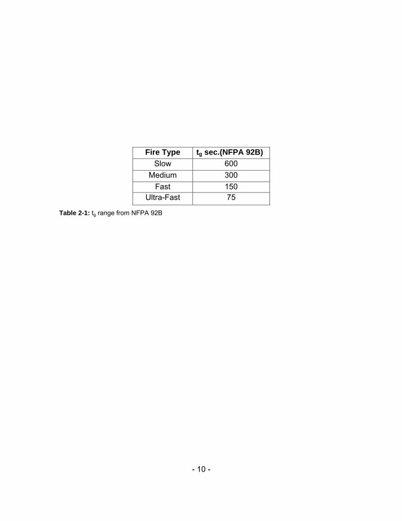
location within a structure. The potential combinations of these effects are infinite, which for design purposes demands that some assumptions be made. To that end, two major time-temperature curves are specified by building codes and are used by engineers in building design: ISO 834 which is the same curve as the 2002 Eurocode Standard Compartment Curve, and ASTM E119 (IBC, 2003). For reference, the ASTM E119 curve represents the combustion of approximately 50kg of wood (with a energy potential of 8.44MJ/kg) per square meter of exposed area per hour of test (Gustaferro, 1987). (See Figure 2-3) These standard curves are often used in the fire testing of structural components, where the component is placed in a furnace and the temperature of the fire is varied according to the applicable time-temperature curve. As implied by the name, however, standard time-temperature curves are generalizations, which are made to allow for performance comparisons between tested structural elements. The curves are agreed-upon approximations by the governing code bodies, and are considered representative of typical compartment fires. The standard curves do not consider specific compartment size, fuel load, material properties, etc., and thus are to be used with caution. 2.2.2 Time-Heat Flux Curves While the protocols for design time-temperature curves are well established, those for time-heat flux histories are not. Code treatment of fire to this point has focused almost exclusively on gas temperature in compartments, thus little attention has been paid to the development of design time-heat flux curves other than the T-squared fires addressed in the next paragraph. Some work has been done by Mangs and Keski-Rahkonen (1994, 2004) at VTT Building Technology in Finland, and Jannsens (2004) at Southwest Research Institute in Texas, USA, in order to parametrize the burning of motor vehicles. The T-squared heat flux curve focuses exclusively on the growth stage of fire history and is still used as a base for growth rate comparison to many actual fires. (See Equation 2-2) It was introduced in the 1980’s as a way to approximate the change in heat-release rate over time as a fire grew. There are four T-squared fire curves: slow, medium, fast, and ultra-fast, which describe the amount of time each fire takes to reach 1055 kW (Fleming, 2003).

- 8 -

2

1055

:eat flux of fire in kW

time after ignition in secondsgrowth time in seconds

g

g

tQt

whereQ htt

⎛ ⎞= ⎜ ⎟⎜ ⎟

⎝ ⎠

===

Equation 2-1: Heat flux equation for T-Squared fires.

Table 2-1 shows the range of tg values set out in the NFPA 92B: Guide for Smoke Management Systems in Malls, Atria, and Large Areas (2005), and Figure 2-2 shows the T-Squared fires plotted versus time. 2.3 ASTM E 119 END POINT CRITERIA As stated in Section 2.2.1, practice for designing structures for fire resistance is governed by codes based on standard fire tests that prescribe specific fire endurance times for structures. In addition to defining a time-temperature standard, the ASTM E 119 tests involve regulations on the end point criteria on which fire resistance duration is based. The end point criteria, specified by ASTM E 119 tests, occurs when: (1) The structure collapses; (2) Holes, cracks, or fissures through which flames or gases can pass form; or (3) The temperature increase of the unexposed surface exceeds an average of 250 degrees Fahrenheit (121.1 degrees Celsius), or a maximum of 325 degrees Fahrenheit (162.7 degrees Celsius) at any one point (PCI Handbook, 1999). Again, the regulations do not consider specific compartment size, fuel load, material properties, etc. Although adhering to the criteria may enable simplicity in design and enforcement of the structure; this approach may be overly conservative in some instances thus resulting in unnecessary costs. 2.4 FIRE MODELING WITH THE FIRE DYNAMICS SIMULATOR With recent advancements in computing techniques and increases in computer power, a growing number of structure fires are being simulated or reconstructed using computer fire models. The computer modeling program used in this project, FDS, was developed at NIST with the objective of solving practical problems in fire protection engineering while providing a tool to study fundamental fire dynamics and combustion. The FDS program is made publicly available free of charge through NIST’s website at http://fire.nist.gov/fds/.

- 9 -

FDS uses a Computational Fluid Dynamics model to simulate fire-drive fluid flow (McGratten, 2005). FDS can be used to model low speed transport of heat and combustion product from fire, radiative and convective heat transfer between gas and solid surfaces, and flame spread and fire growth. The program calculates the net heat flux into a surface as a combination of the radiative and convective heat flux. The convective heat flux equation used is displayed in Equation 2-2.

c

c

g

w

q" ( )

:q" convective heat flux

convection coefficientT gas temperature

T wall temperature

g wh T T

where

h

= −

=

==

=

&

&

Equation 2-2: FDS net heat flux equation. FDS solves numerically a form of the Navier-Stokes equations for low-speed (incompressible) flow. The Navier-Stokes equations are a set of five, non-linear second-order partial differential equations that are derived from the conservation of mass, momentum, and energy equations, the ideal gas law, and the equation for density in any particular volume element (Bayreuther, 2006). Because the rate of fluid flow (convection) is small in comparison to the speed of sound, the fluid in the fire analyses is assumed to be compressible, thus allowing for the fifth Navier-Stokes equation to be dropped. In vector notation, the Navier-Stokes equations are:

( )v v v F p vt

ρ μ∂⎛ ⎞⋅ + ⋅∇ = −∇ + ⋅Δ⎜ ⎟∂⎝ ⎠

Equation 2-3: Vector Notation of the Navier-Stokes Equations. The FDS radiative heat flux calculations are conducted following a version of the finite volume method for convective transport which is used to solve the radiation transport equations for gray gas. A complete discussion can be found in Section 3.3 of the FDS Technical Reference Guide (McGratten, 2005).

- 10 -

Fire Type tg sec.(NFPA 92B) Slow 600

Medium 300 Fast 150

Ultra-Fast 75

Table 2-1: tg range from NFPA 92B

- 11 -

0

200

400

600

800

1000

1200

0 20 40 60 80 100 120

Time (min.)

Tem

p (d

eg. C

) Eurocode Standard CompartmentCurve (ISO 834)Eurocode Hydrocarbon Curve

Eurocode ParametricCompartment CurveASTM E119 Standard Curve

Figure 2-1: Standard time-temperature comparisons; Eurocode Standard (ISO834), ASTM E119, Eurocode External, Eurocode Hydrocarbon, Eurocode parametric curve for parking garage model (Bayreuther, 2006).

0

200

400

600

800

1000

1200

0 100 200 300 400 500 600

Time (sec)

HR

R (k

W)

SlowMediumFastUltra-Fast

Figure 2-2: T-Squared fires from NFPA 92B (2005) (Bayreuther, 2006).

- 12 -

CHAPTER 3

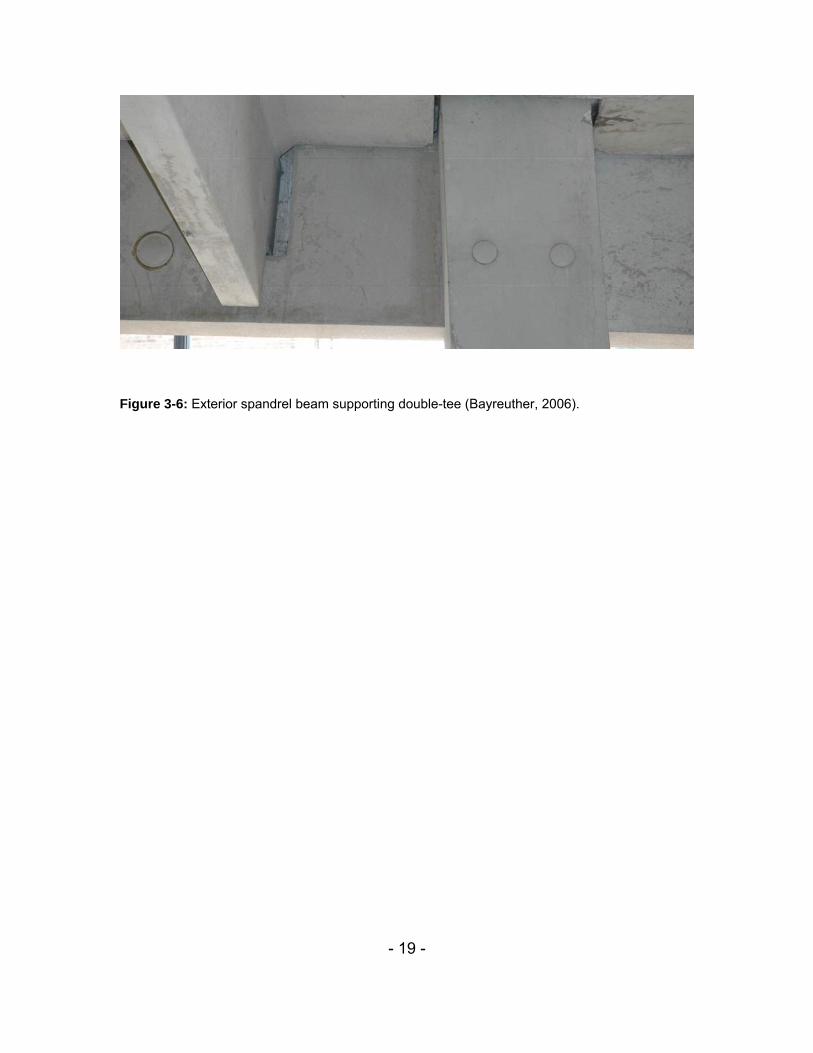
PROTOTYPE STRUCTURE AND ANALYSIS MATRIX This chapter presents a description of the prototype structure and analysis matrix. Section 3.1 discusses the structure that the analysis models are based on. Section 3.2 introduces the analysis models, with Section 3.2.1 describing the parking garage model and Section 3.2.2 detailing the vehicle model and fire characteristics. The fire analyses conducted in this project are presented in Section 3.3. Section 3.3.1 provides a summary of the analyses. Sections 3.3.2 and 3.3.3 provide descriptions of the analysis variables. 3.1 PROTOTYPE STRUCTURE DESCRIPTION The analysis models were constructed to represent the Lehigh University Campus Square Parking Garage Structure shown in Figures 3-1 and 3-2. Bayreuther (2006) presents a detailed description of the prototype structure used to conduct the analyses. Because this research is a continuation of that work, models were based off of the same prototype structure. The following is a summary of Bayreuther (2006). The prototype structure, the Campus Square Parking Garage, is located on a sloping lot with three floors above grade on the south side and four on the north side. The floor height varies from 3.8m on the ground floor to 3.1m for each of the upper floors. Overall dimensions are 45m from east to west and 36m from north to south. The garage is constructed of precast, prestressed concrete double-tees that are oriented longitudinally north-to-south, and three double-tees are placed side-by-side in between each column forming bays. The typical double-tee used is similar to the 15DT34 design from the PCI Handbook (2004), which is 4.6m wide, 18.4m long, and 0.87mm in total depth (Figure 3-3). The double-tees are simply supported on the interior walls by inverted-tee girders (Figure 3-4) or corbels (Figure 3-5) protruding from the center shear wall. The exterior ends of the double-tees are supported by a spandrel beam with pockets to allow the webs at the end of the double-tee to rest in a simply supported manner (Figure 3-6). Precast sections also comprise the center shear wall, which includes a series of larger openings. Driving ramps to allow vehicles to move between floors are created by inclining double-tee sections. An as built drawing of one-floor of the Campus Square Parking Garage is shown in Figure 3-7.

- 13 -

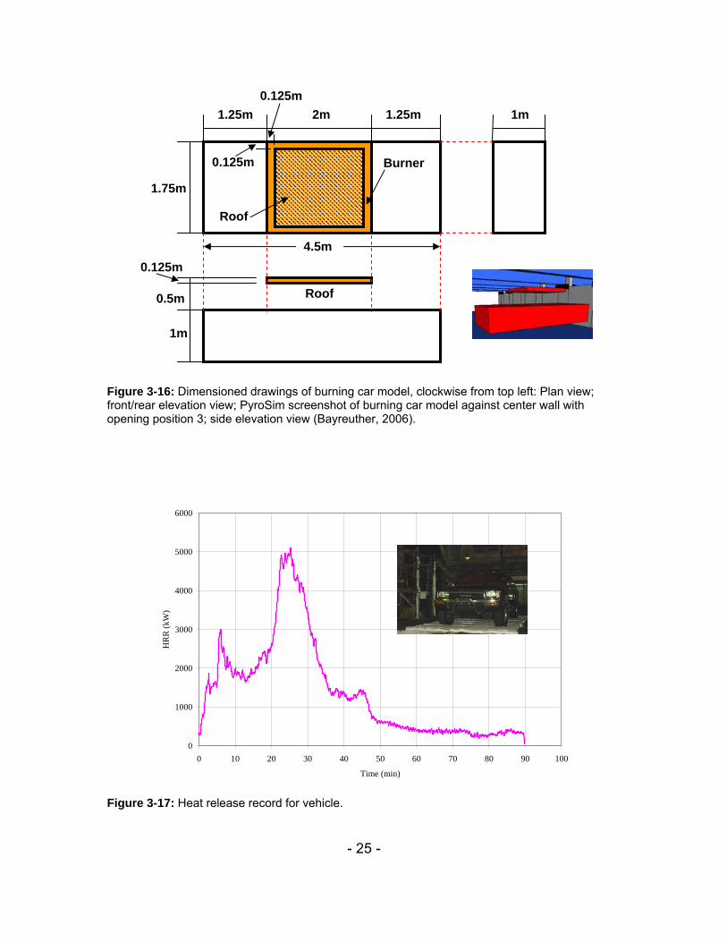
3.2 ANALYSIS MODEL The model used for the analyses was created based on the prototype structure discussed in Section 3.1. Section 3.2.1 discusses the parking garage analysis model and Section 3.2.2 discusses the vehicle model and fire characteristics. 3.2.1 Parking Garage Analysis Model The parking garage model was created using PyroSim (a graphical pre-processor to FDS that will be explained in Chapter 4). As was discussed in Chapter 2, the FDS program was used to run the analyses and submit output files. One of the main requirements of the FDS software is that the models must be constructed with a uniform computational mesh. As a result, the mesh cells had to have the same length, width, and height. Additionally, building scale models in FDS require cell sizes of 0.100m to 0.150m for reasonable accuracy. As discussed in Bayreuther (2006), through trial and error attempts, 0.125m cells were found to most accurately capture the geometry of the structure. In order to conform to the FDS constraints, a 0.125m cubic mesh was used to create the model, and every measurement in the model was constrained to 0.125m increments. Figure 3-8 shows cross-sections of a single double-tee overlaid with a 0.125m mesh. Again, because of the uniform mesh constraint, all other elements of the parking garage structure, including columns, corbels, and floor height, had to adhere to the 0.125m cubic mesh. Figures 3-9 to 3-14 show dimensioned figures of the parking garage model used for the analyses. 3.2.2 Vehicle Model and Fire Characteristics In order to provide for accurate comparisons to be made from the results of the analyses completed in this project with the results of the analyses completed by Bayreuther (2006), the vehicle model and fire characteristics remained unchanged. The following is extracted from Bayreuther (2006). Vehicle Model Like the approximations that were made to create the model of the parking garage, the vehicle model geometry was also simplified in order to conform to the 0.125m mesh and to match the fire behavior exhibited during actual testing performed by Khono et al (2004). The vehicle model is intended to represent a typical midsize passenger vehicle, and all surfaces in the model are considered to be inert. The dimensions are approximations of a 2004 Ford Taurus. Other

- 14 -

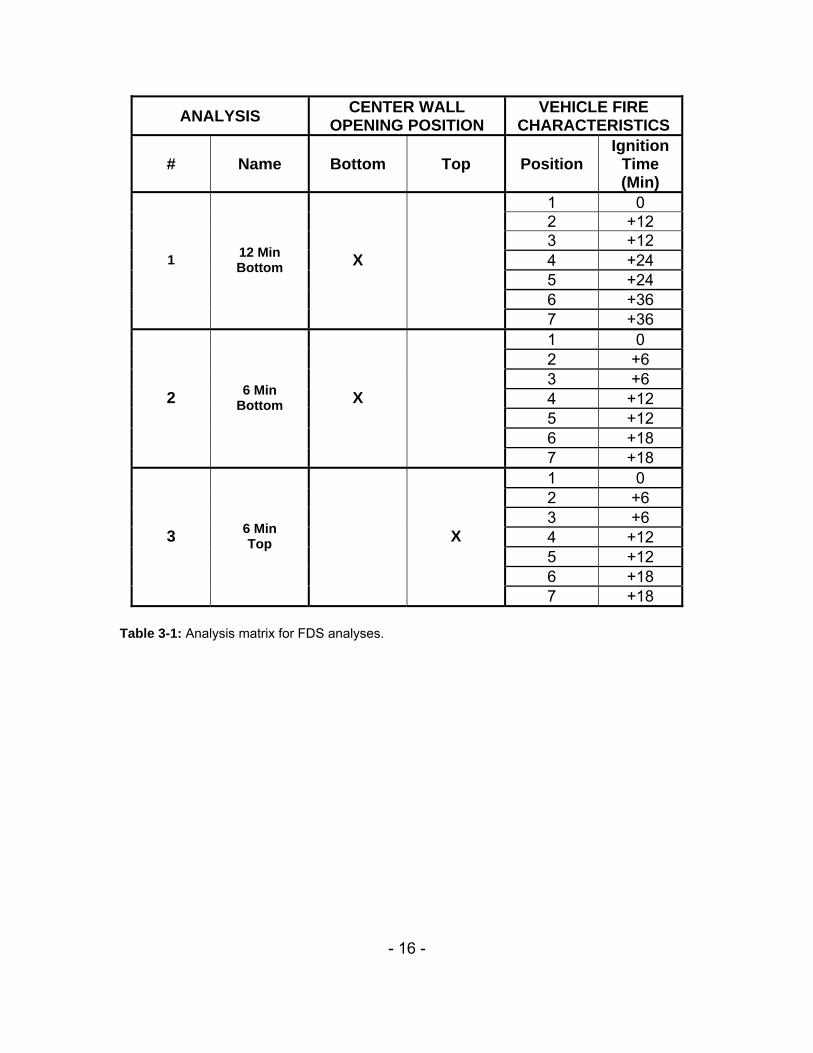
vehicles in this class include: Toyota Camry, Honda Accord, Dodge Stratus, and BMW 5-Series. As shown in Figures 3-15 and 3-16, the body of the vehicle is approximated by a rectangular prism, 4.5m long, 1.75m wide, and 1m high. A 0.125m thick plate 1.75m long and 1.5m side is centered 0.5m over the body to represent the roof of the cab of the vehicle. Fire Characteristics The fire is modeled in FDS as a flat surface called a burner, and is distributed over the area that would be taken up by the cab in a real vehicle as shown in the model. The burner was modeled as a flammable solid vent with a given heat flux release rate input. Figure 3-17 shows the heat flux release record chosen as the input to the model. The area under the time-heat release curve is defined as the total energy output recorded during the analysis, which for this vehicle is 7387 MJ. Based on research conducted by Bayreuther, the specific vehicle was chosen because its heat flux record had a total energy release and heat flux in the upper range of the data shown previously in Figure 2-2. 3.3 FIRE ANALYSES The focus of this research was to expand upon the matrix of fire analyses conducted by Bayreuther (2006) to further investigate the effects of fire loading on precast concrete parking structures. A full description of the analyses previously conducted can be found in Section 3.2 of Bayreuther (2006). The following section presents the analysis matrix and explains the variables addressed in this project. 3.3.1 Analysis Matrix Three multi-vehicle fire analyses were performed to address two variables and investigate heat transmission throughout the structure. Table 3-1 summarizes the analyses which are described in Sections 5.2.1 through 5.2.3. The two variables addressed in this project were ignition time between vehicles and center wall opening position of the parking structure. The following sections, Sections 3.3.2 to 3.3.3 explain the variables addressed in the analyses. 3.3.2 Analysis Variable: Vehicle Ignition Time The title of this analysis variable, ‘Vehicle Ignition Time’, is used to describe the ignition time of each of the vehicles in the analyses. Analyses 1 and 2 were created in order to investigate the effects varying this ignition time had on heat

- 15 -

transmission through the structure. The models were populated with vehicles in a parking pattern typical of that of the prototype structure. As shown in Figure 3-18, this pattern causes the relative position of the vehicles in relation to the webs of the double-tees to vary. In each of the analyses, a total of seven vehicles ignite on a single floor. The pattern of ignition for Analysis 1, which will be referred to as ‘12 Min Bottom’ for the duration of this report, is as follows: The vehicle in position 1 (Vehicle 1, Figure 3-18) ignites at time 0, Vehicles 2 and 3 ignite at time +12 minutes, Vehicles 4 and 5 ignite at time +24 minutes, and Vehicles 6 and 7 ignite at time +36 minutes. In Analysis 2, which will be referred to as ‘6 Min Bottom’ for the duration of this report, the ignition times of vehicles 2 though 7 are halved. In 6 Min Bottom, Vehicle 1 ignites at time 0, Vehicles 2 and 3 ignite at time +6 minutes, Vehicles 4 and 5 ignite at time +12 minutes, and Vehicles 6 and 7 ignite at time +18 minutes. 3.3.3 Analysis Variable: Center Wall Opening Position The center wall opening position of the prototype structure is comprised of precast concrete sections with large openings regularly spaced (Figure 3-19). As previously stated, the double-tees are inclined in order to create driving ramps through the floors. Because of the inclination of the double-tees, the relative position of the center wall openings varies in relation to the floor slab along the length of the garage (also shown in Figure 3-19). The openings in the center wall allow combustion gases to pass from one side of the garage to the other and potentially from one floor to the next depending on the elevation of the double-tees relative to the openings (Bayreuther, 2006). In order to investigate the effect of opening position on heat transmission through the structure, two different opening positions of the center wall in relation to the floor slab were modeled. The first opening position of the center wall is referred to as ‘bottom’ and the second opening position of the center wall is referred to as ‘top’. In both 12 Min Bottom and 6 Min Bottom, the bottom center wall opening position is flush with the top of the floor slab (Figure 3-20). In the third analysis, referred to as ‘6 Min Top’, the top of the center wall opening is flush with the bottom of the floor slab that forms the ceiling (Figure 3-21). As previously stated, because of the inclination of the double-tees, neither the bottom opening or top opening center wall position is present in the prototype garage, but both are possible scenarios for such a structure.

- 16 -

ANALYSIS CENTER WALL OPENING POSITION

VEHICLE FIRE CHARACTERISTICS

# Name Bottom Top Position Ignition

Time (Min)

1 0 2 +12 3 +12 4 +24 5 +24 6 +36

1 12 Min Bottom X

7 +36 1 0 2 +6 3 +6 4 +12 5 +12 6 +18

2 6 Min Bottom X

7 +18 1 0 2 +6 3 +6 4 +12 5 +12 6 +18

3 6 Min Top X

7 +18 Table 3-1: Analysis matrix for FDS analyses.

- 17 -

Figure 3-1: Lehigh University Campus Square parking garage (southwest corner) (Bayreuther, 2006).

Figure 3-2: Lehigh University Campus Square parking garage (southeast corner) (Bayreuther, 2006).

- 18 -

Figure 3-3: 15DT34 Double-tee from PCI Handbook (2004).

Figure 3-4: Inverted-tee spandrel supporting double-tee (Bayreuther, 2006).

Figure 3-5: Corbels supporting double-tee (Bayreuther, 2006).

1149.3mm 2.3m 1149.3mm

4.6m

230mm

76.6mm

166mm

102mm

868.4mm

1149.3mm 2.3m 1149.3mm

4.6m

230mm

76.6mm

166mm

102mm

868.4mm77mm

2300mm 1150mm

868mm

1150mm

- 19 -

Figure 3-6: Exterior spandrel beam supporting double-tee (Bayreuther, 2006).

- 20 -

Figure 3-7: Lehigh University Campus Square parking garage: example of as-built drawing (Bayreuther, 2006).

- 21 -

Figure 3-8: Double-tee approximation for 0.125m cell size. (A) Actual 15DT34; (B) 0.125m approximation; (C) Overlay of (A) and (B).

Figure 3-9: Single double-tee approximation used in the FDS model with dimensions shown (units in meters).

1 0.25 2

0.75

A

B

C

0.125m

0.125

- 22 -

22.5

36.75

Double-tee webs

Center wall

22.5

36.75

22.5

36.75

Double-tee webs

Center wall

Figure 3-10: Plan View of FDS model (units in meters).

0.25

0.25

0.25 18180.25 0.25

3

7.75

0.2536.75

0.25

1.75

0.125

0.75

Double-tee

Center wall

Corbel Column

0.25

0.25

0.25 18180.25 0.25

3

7.75

0.2536.75

0.25

1.75

0.125

0.75

0.25

0.25

0.25 18180.25 0.25

3

7.75

0.2536.75

0.25

1.75

0.125

0.75

Double-tee

Center wall

Corbel Column

- 23 -

Figure 3-11: East-West elevation view of FDS model (units in meters).

1.75

1.75

1.75

1.25

1.25

22.5

4 1 12.5 1 4

1.75

Spandrel

Column1.75

1.75

1.75

1.25

1.25

22.5

4 1 12.5 1 4

1.75

1.75

1.75

1.75

1.25

1.25

22.5

4 1 12.5 1 4

1.75

Spandrel

Column

Figure 3-12: North-South elevation view of FDS model (units in meters).

22.5

0.125

2.875

2.875

21

0.25

0.125

0.75

Double-tee webs

Corbels

22.5

0.125

2.875

2.875

21

0.25

0.125

0.75

Double-tee webs

Corbels

Figure 3-13: North-South elevation view of FDS model showing double-tees and corbels (units in meters).

- 24 -

1.75

1.75

1.25

1.25

22.5

0.75 0.751.5

Center wall openings

1.75

1.75

1.25

1.25

22.5

0.75 0.751.5

1.75

1.75

1.25

1.25

22.5

0.75 0.751.5

Center wall openings

Figure 3-14: North-south elevation view of FDS model showing center wall (units in meters).

Figure 3-15: (A) Actual outline of a 2000 Ford Taurus; (B) 0.125m approximation used for FDS modeling; (C) Overlay of (A) and (B) (Bayreuther, 2006).

A

B

C

- 25 -

Figure 3-16: Dimensioned drawings of burning car model, clockwise from top left: Plan view; front/rear elevation view; PyroSim screenshot of burning car model against center wall with opening position 3; side elevation view (Bayreuther, 2006).

0

1000

2000

3000

4000

5000

6000

0 10 20 30 40 50 60 70 80 90 100

Time (min)

HR

R (k

W)

Figure 3-17: Heat release record for vehicle.

4.5m

1m

1.75m

Roof

1m

0.5m 0.125m

1.25m 2m 1.25m

Roof

Burner0.125m

0.125m

- 26 -

Figure 3-18: Location of vehicles and position numbers.

124 3 56 7

- 27 -

Figure 3-19: Image of the center wall of the prototype garage (Bayreuther, 2006).

Figure 3-20: View of the bottom opening center wall position.

Figure 3-21: View of the top opening center wall position.

Center Wall

Opening (Bottom)

Slab

Web

Slab

Web

Center Wall

Opening (Top)

- 28 -

CHAPTER 4

FIRE ANALYSIS PROCEDURE

This chapter explains the procedure used to conduct the fire analyses. Section 4.1 gives an overview of the analysis procedure. Section 4.2 describes the process of constructing the parking garage models through use of an interactive graphical preprocessor (PyroSim). Section 4.3 explains the use of FDS, the computer program that solves equations to complete the analyses. Section 4.4 gives an explanation of the analysis output. 4.1 OVERVIEW OF ANALYSIS PROCEDURE The objective of the fire analysis was to simulate various multiple-vehicle fires on a single floor of the parking garage and determine the resulting gas temperatures and heat flux throughout the structure. Plots of gas temperatures over time are useful for comparing different fires; and knowledge of heat flux is necessary to determine the temperature rise of the structure’s components. In order to obtain the gas temperatures and heat flux data from each analysis, a procedure utilizing multiple computer programs was performed. The following sections detail the sequential steps of the analysis procedure. 4.2 CREATING THE ANALYSIS MODEL The parking garage models were built using PyroSim, a graphical interface that serves as a preprocessor to FDS (as discussed in Chapter 2, FDS is the computer program used to compute the gas temperatures and heat flux values). In addition to assembling the models, a number of material properties and analysis parameters had to be specified in PyroSim. The following two sections, 4.2.1 and 4.2.2, detail the material properties and analysis parameters specified in PyroSim for this project. 4.2.1 Concrete Material Properties The entire model of the parking garage was assigned the properties of concrete as explained below. Surface Type:

Non-Flammable Solid

- 29 -

Properties: Emmisivity: 0.6 Backing: FDS allows three backing conditions: (1) Air-gap, which is used for hollow walls such as gypsum board over wood studs; (2) Insulated, which is used for similar situation as the air-gap condition but includes insulation in the void; and (3) Exposed, which is used when the back of the obstruction is exposed and allows a one dimensional heat transfer though the thickness of the obstruction as long as the obstruction is only one cell thick. In both the air-gap and insulated cases, FDS does not compute heat transfer through the obstruction. (Note: Any solid object in FDS is referred to as an obstruction.) Because it allows for heat to transfer through the material (which most realistically models the fire scenario), Exposed was selected as the backing condition.

Boundary Conditions:

Surface Type: FDS allows four thermal boundary conditions: (1) Fixed temperature solid surface; (2) Fixed heat flux solid surface; (3) Thermally thick solid; and (4) Thermally thin sheet. The thermally thick condition was chosen for this project because it is the only condition that allows the user to prescribe thermal properties of the material. Thermal Conductivity: The thermal conductivity of the material could either be specified as a constant value, or allowed to vary with temperature. Because the thermal conductivity of concrete varies with temperature, the second option was chosen. Figure 4-1 shows the temperature-thermal conductivity plot that was used as the thermal conductivity input. Specific Heat: The specific heat could also either be specified as a constant value, or allowed to vary. Because the specific heat of concrete varies with temperature, the second option was chosen. Figure 4-2 shows the temperature-specific heat plot that was used as the specific heat input. Density: 2100 kg/m3

4.2.2 Analysis Parameters In addition to the material properties, there are a number of analysis parameters that must be selected in PyroSim. The parameters chosen for the fire analyses of this project are explained in this section. Time:

Duration: The total duration of each analysis was 5760 seconds. The multiple car burns were constructed of a series of 3600 second single car burns with a ΔT offset of 12 minutes (720 seconds). 3600 seconds was chosen as the duration of a single vehicle fire because all of the car burn tests that the HRR data were taken from are essentially over at about the one hour mark. 12 minutes was chosen as the ΔT offset in 12 Min Bottom

- 30 -

because the fire spread in both Steinert (2000) and Mangs (1994) generally fell within 4 to 15 minutes. Again, like the car fire records, the literature did not provide enough data to point to a conclusive ΔT, and a choice was made to estimate the time at 12 minutes. 6 Min Bottom used 6 minutes as the ΔT offset to investigate the effects this variation would have on the heat transfer. Initial Time Step: The FDS solver default value of 1E-02 seconds was specified. Number of output frames: The FDS default value of 1000 frames was specified.

Environment:

Ambient Temperature: The FDS default value of 20 degrees Celsius was chosen. Ambient Pressure: The FDS default value of 1.01325E5 Pa was chosen. Initial Wind Velocity: No wind was included in this study.

Simulator:

Non-Isothermal Calculation: (YES) Enable Radiation Transport Solver: (YES) – In FDS, one has the option of turning off the radiation transport solver within the program in order to speed up computation times if the radiation quantity is not needed. For this project radiation was a critical computed quantity, thus the solver was turned on. Simulation Type: FDS can run fluid dynamics calculations using either Direct Numerical Simulation or Large Eddy Simulation. Direct Numerical Simulation is only useful for very fine meshes (usually 1mm or less) and requires a large computation effort. Large Eddy Simulation solves the partial differential equations governing fluid flow, and requires much less computation effort. Large Eddy Simulation was chosen for this project.

Boundary Conditions:

Boundaries for the model are defined in the FDS model as large, open vents that allow heat and combustion materials to exit the model but not return. They define the extents of the computational domain and are placed on all six sides of the model.

4.3 RUNNING THE FIRE ANALYSIS After all of the material properties and analysis parameters were specified, the PyroSim software generated a text file containing the input parameters needed to run the fire analysis. As discussed in Chapter 2, the Fire Dynamics Simulator is the computer program that was used to conduct the fire analyses. The FDS program reads the input parameters, numerically solves equations governing

- 31 -

liquid and gas flow, and writes two types of output data to files. The output data is discussed in Section 4.4. If the text file generated by PyroSim is small enough, the FDS program can efficiently run it on a single processor. However, due to the large size and intricacy of the models in this project, multiple computer processors were utilized. The use of multiple computer processors to run an analysis, termed “multi-blocking” was the technique also used in the work conducted by Bayreuther (2006) to decrease the amount of computing time required to run the models. The following description of multi-processor computing with FDS was extracted from Bayreuther (2006). Multi-blocking, or the use of multiple computer processors to run an FDS analysis significantly decreases the amount of time required to run each model. Multi-blocking divides the model into essentially separate sections that are coupled together in the FDS code. Each section or ‘block’ is run on a separate processor, so a model of 2000 cells run on 4 processors might be blocked evenly into 4 blocks of 500 cells. Uneven multi-blocking is also possible and may be used to create finer meshes in critical sections of a model while using more coarse meshes in other portions. A thorough explanation of multi-blocking schemes is available in the FDS User’s Guide (2005), and Minkowycz (2000) also discusses the mathematical implications of CFD model division. For each analysis, the blocking scheme for the model was chosen to be basic while trying to keep block boundaries away from direct contact with flame wherever possible. Four processors were available on the computing cluster, so the model was divided into four blocks as shown in Figure 4-3. In order to conform to the FDS computational constraints, the block dimensions had to be multiples of 2, 3, and 5 because of the Fast Fourier Transforms used in the calculations. Subsequently, each block was 180 cells in the x-direction, 80 cells in the y-direction, and 24 cells in the z-direction for a cell subtotal of 345,600 cells for each block and a total of 1,382,400 cells for the entire model. 4.4 FDS OUTPUT DATA Before an FDS analysis is run, the output data must be specified. In order to capture gas temperatures at a single point in the structure throughout the entire duration of the analysis, thermocouples were placed throughout the model at key locations. The locations of the thermocouples were specified in PyroSim, and are shown in Figure 4-4. The thermocouples recorded gas temperature measurements in 30 second increments for the duration of the analysis, which allowed this quantity to be plotted as a function of time (See Chapter 5).

- 32 -

In addition to the thermocouple data, gas temperatures were also recorded along a plane or “slice” of the model. The locations of the slice files were chosen at critical planes in the model, and are shown in Figure 4-5. Using Smokeview, a post-processor to FDS, data recorded by the slice files was able to be displayed graphically (as shown in Chapter 5). The second type of output returned by FDS is boundary files. Boundary files record surface quantities at all solid obstructions. For this research, heat flux data was gathered by boundary files. The heat flux data recorded by the boundary files was used as the input to a non-linear heat transfer finite element analysis that is presented in Chapter 7.

- 33 -

0

0.2

0.4

0.6

0.8

1

1.2

1.4

1.6

0 100 200 300 400 500 600 700 800 900 1000

Temperature (Deg. C)

Ther

mal

Con

duct

ivity

(W/(m

*K))

Figure 4-1: Thermal conductivity of concrete.

0

500

1000

1500

2000

2500

3000

0 100 200 300 400 500 600 700 800 900 1000

Temperature (Deg. C)

Spec

ific

Hea

t (kJ

/(kg*

K)

Figure 4-2: Specific heat of concrete.

- 34 -

Figure 4-3: Blocking layout for FDS models.

Figure 4-4: Plan view of thermocouple locations at z = 3.625m. All dimensions in meters.

- 35 -

Figure 4-5: Plan view of slice file locations. All dimensions in meters.

- 36 -

CHAPTER 5

INDIVIDUAL FIRE ANALYSIS SUMMARIES

This chapter presents results of each of the fire analyses. The procedure followed to determine the results was described in Chapter 4. Each of the three analysis summaries is presented in a similar format which is explained in section 5.1. Section 5.2 contains the individual summaries for each of the three analyses: 12 Min Bottom, 6 Min Bottom, and 6 Min Top. 5.1 FORMAT OF ANALYSIS SUMMARIES Each individual analysis summary is presented in the format as described below.

1. A description of the geometry and fire properties of the model. 2. A description of the heat movement through the structure over

the course of the analysis, with reference to slice file images and time-temperature figures.

3. Figures of the model. 4. Slice file images obtained from Smokeview showing the heat

distribution through the structure. 5. Plots of time-temperature histories showing the thermocouple

records for locations of interest. 5.2 INDIVIDUAL FIRE ANALYSIS SUMMARIES The following sections present the results of each of the individual analyses. 5.2.1 12 Min Bottom Analysis Figures 5-1 and 5-2 show the geometry of the 12 Min Bottom Analysis model (Bayreuther, 2006). The model consists of a total of seven vehicles in sequential ignition on a single floor. The time duration between ignitions of adjacent vehicles is 12 minutes. Initially, the vehicle in position 1 ignites, followed by Vehicles 2 and 3 at ΔT = +12 minutes, Vehicles 4 and 5 at ΔT = +24 minutes, and Vehicles 6 and 7 at ΔT = +36 minutes, as shown in Figure 5-3. As was shown in Figure 5-1, Vehicle 1 is centered in between the double-tee stems. The figure also displays the position of the center wall opening, located flush with the top of the double-tee slab. Slice images of temperature created by Smokeview are shown in Figure 5-5. The images display the temperature distribution through the structure 0.125m below

- 37 -

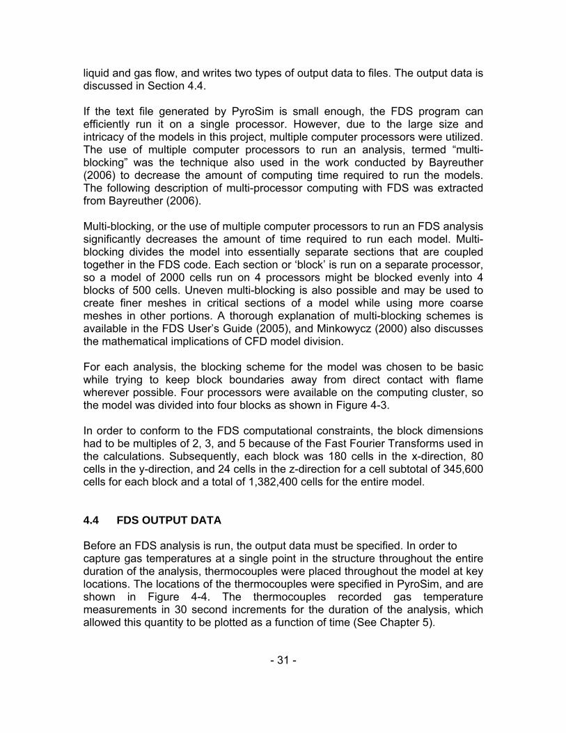
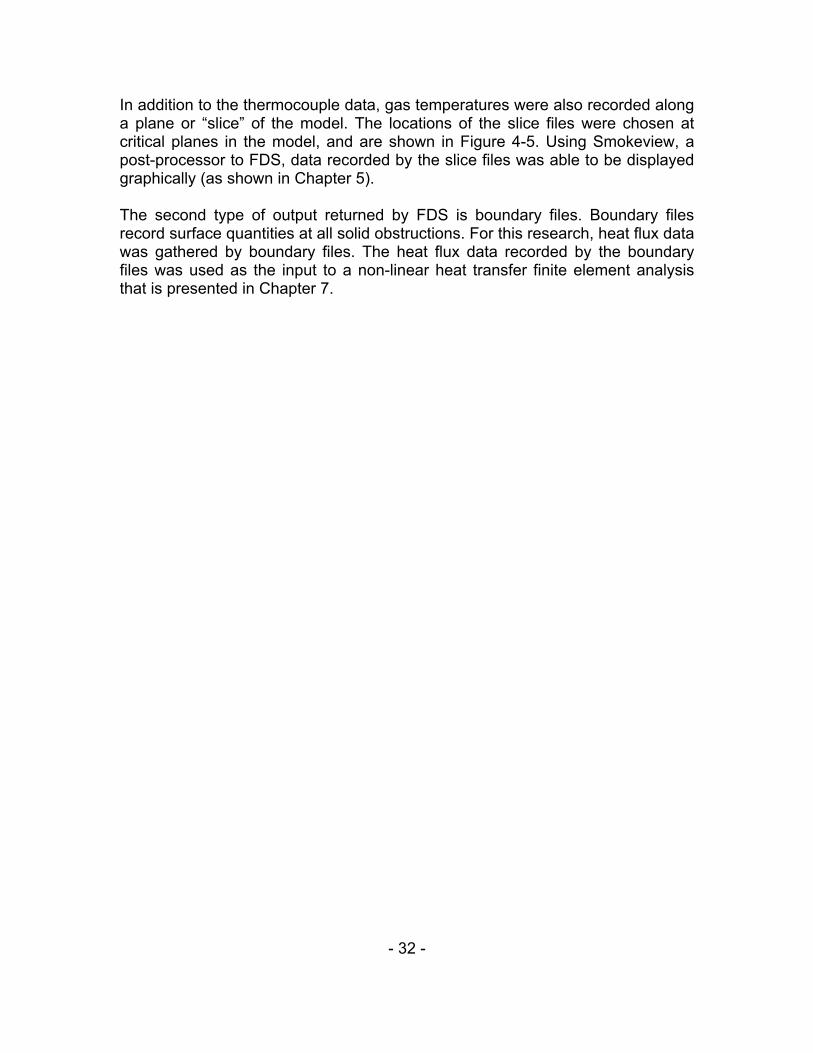
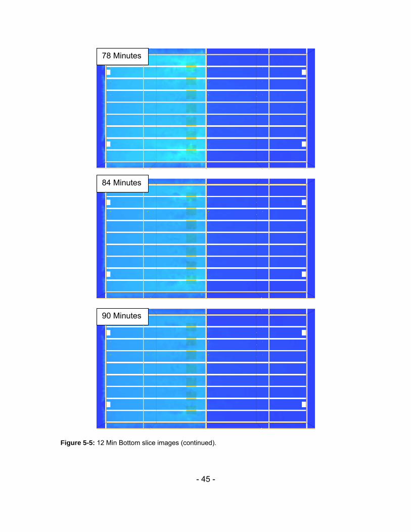
the slab (Figure 5-4). Images were captured in 6 minute intervals and were calculated for the entire duration of the analysis. The images of Figure 5-5 show the buildup of heat longitudinally throughout the garage with some of the heat flowing underneath the double-tee webs and encompassing the adjacent double-tee web cavity. Very little to no heat is observed traveling through the center wall opening to the opposite side of the model. Time-temperature histories recorded by thermocouples throughout the structure are plotted in Figures 5-7 to 5-12. The plots display gas temperature histories for the duration of the analysis (5760sec). Figures 5-7 to 5-9 show longitudinal time-temperature plots, while Figures 5-10 to 5-12 show transverse time-temperature plots. Figure 5-6 shows a plan view of the location key for thermocouples in the x and y directions. All thermocouples were located at a distance 3.625m above the z axis. Figure 5-7 is a graph of the time-temperature histories calculated at four thermocouples located along the length of the flange above burning Vehicle 1 from y = 0.25m to y = 18m. The greatest temperatures observed were 728 and 897 degrees Celsius at y = 18m and y = 15.25m, respectively. The plots from the thermocouples located at y = 9m and y = 0.25m show that as the distance from the center of the fire increased, the gas temperatures generally decreased. Figure 5-8 is a graph of the time-temperature histories recorded by four thermocouples located along the length of the flange on the other side of the center wall, opposing burning Vehicle 1. The drastic decrease in temperatures (in comparison to those of Figure 5-7) indicates that very little heat flows through the center wall opening to the opposite side of the structure. This result is further demonstrated by Figure 5-9 which shows the time-temperatures plots from the thermocouples located on either side of the center wall. The temperatures recorded from the side of the wall in which the vehicles are burning are significantly higher than those recorded 0.75m away on the opposite side. Figures 5-10, 5-11, and 5-12 are plots of time-temperature histories from thermocouples located at varying x coordinates throughout the structure. The plots show that some heat from each vehicle fire flows underneath the double-tee webs to the adjacent cavity, but the majority of the heat is contained within the cavity above the burning vehicle. The maximum temperature reached during the analysis was 983 degrees Celsius, recorded by the thermocouple located at the coordinates of x = 9.0m, y = 15.25m, and z = 3.625m, shown in Figure 5-10. The peak temperature was reached approximately 35 minutes (2100sec) after ignition of Vehicle 1, 22

- 38 -

minutes (1320sec) after ignition of Vehicle 2, 33 minutes (660sec) after ignition of Vehicle 4, and 1 minute (60sec) before ignition of Vehicle 6.

- 39 -

Figure 5-1: 12 Min Bottom model showing burning vehicles and center wall opening position.

Figure 5-2: 12 Min Bottom model (plan view).

- 40 -

12 4 3 56 7

Figure 5-3: 12 Min Bottom vehicle numbers and ignition times.

Figure 5-4: Location of slice 0.125m below the slab. Temperature scale in degrees Celsius.

Vehicle Ignition Time (min)

1 0 2,3 12 4,5 24 6,7 36

Slice images shown 0.125m below slabSlice images shown 0.125m below slab Slice images shown 0.125m below slab

- 41 -

Figure 5-5: 12 Min Bottom slice images showing temperature distribution throughout the structure.

6 Minutes

12 Minutes

18 Minutes

- 42 -

Figure 5-5: 12 Min Bottom slice images (continued).

24 Minutes

30 Minutes

36 Minutes

- 43 -


42 Minutes

48 Minutes

54 Minutes

- 44 -


60 Minutes

66 Minutes

72 Minutes

- 45 -


78 Minutes

84 Minutes

90 Minutes

- 46 -

Figure 5-5: 12 Min Bottom slice image (continued).

y = 0.25m

y = 3my = 9m

y = 15.25m

y = 18m

y = 18.75m

y = 21m

y = 27.5m

y = 36.25m

x = 0m

x = 4.5mx = 6.75mx = 9mx = 11.25m

x

y

y = 0.25m

y = 3my = 9m

y = 15.25m

y = 18m

y = 18.75m

y = 21m

y = 27.5m

y = 36.25m

x = 0m

x = 4.5mx = 6.75mx = 9mx = 11.25m

x

y

Figure 5-6: 12 Min Bottom location key for thermocouples.

96 Minutes

- 47 -

0100200300400500600700800900

100011001200130014001500

0 1200 2400 3600 4800

Time (sec)

Tem

pera

ture

(deg

. C)

y = 0.25my = 9.0my = 18.0my = 15.25m

Figure 5-7: 12 Min Bottom time-temperature histories centered between double-tee webs above burning vehicle at x = 11.25m; y = 0.25m, 9.0m, 15.25m, 18.0m; z = 3.625m.

0100200300400500600700800900

100011001200130014001500

0 1200 2400 3600 4800

Time (sec)

Tem

pera

ture

(deg

. C)

y = 18.75my = 21.0my = 36.25my = 27.5


y = 0.25m y = 9.0m

y = 15.25m

y = 18.0m

y = 18.75m y = 21.0m

y = 27.5m y = 36.25m

- 48 -

0100200300400500600700800900

100011001200130014001500

0 1200 2400 3600 4800

Time (sec)

Tem

pera

ture

(deg

. C)

y = 18.0m

y = 18.75m

Figure 5-9: 12 Min Bottom time-temperature histories centered between double-tee webs above burning vehicle at x = 11.25m; y = 18.0m, 18.75m; z = 3.625m.

0100200300400500600700800900

100011001200130014001500

0 1200 2400 3600 4800

Time (sec)

Tem

pera

ture

(deg

. C)

x = 11.25m

x = 9.0m

x = 6.75m

Figure 5-10: 12 Min Bottom time-temperature histories centered between double-tee webs above burning vehicle at x = 11.25m, 9.0m, 6.75m; y = 15.25m; z = 3.625m.

y = 18.0m y = 18.75m

x = 11.25m x = 9.0m x = 6.75m

- 49 -

0100200300400500600700800900

100011001200130014001500

0 1200 2400 3600 4800

Time (sec)

Tem

pera

ture

(deg

. C)

x = 11.25mx = 9.0mx = 6.75m


0100200300400500600700800900

100011001200130014001500

0 1200 2400 3600 4800

Time (sec)

Tem

pera

ture

(deg

. C)

x = 11.25m

x = 9.0m

x = 6.75m


x = 11.25m x = 9.0m x = 6.75m

x = 11.25m x = 9.0m x = 6.75m

- 50 -

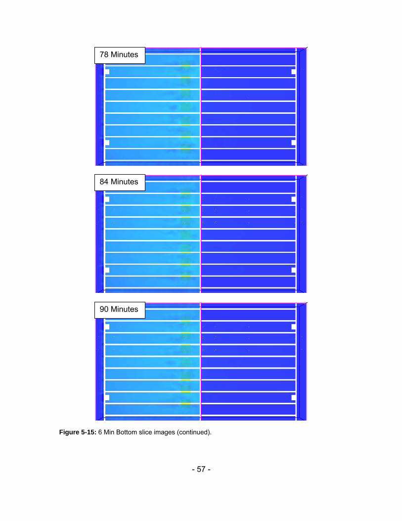
5.2.2 6 Min Bottom Analysis The purpose of 6 Min Bottom was to investigate the effect reducing the time duration between ignitions of adjacent vehicles had on the heat flow throughout the structure. The geometry of the 6 Min Bottom model is identical to that of the 12 Min Bottom model shown in Figures 5-1 and 5-2. The model consists of a total of seven vehicles in sequential ignition on a single floor. The time duration between ignitions of adjacent vehicles is 6 minutes. Initially, the vehicle in position 1 ignites, followed by Vehicles 2 and 3 at ΔT = +6 minutes, Vehicles 4 and 5 at ΔT = +12 minutes, and Vehicles 6 and 7 at ΔT = +18 minutes, as shown in Figure 5-13. As was shown in Figure 5-1, Vehicle 1 is centered in between the double-tee stems. The figure also displays the position of the center wall opening, located flush with the top of the double-tee slab. Slice images created using Smokeview are shown in Figure 5-15. The images display the temperature distribution through the structure 0.125m below the slab (Figure 5-14). Images were captured in 6 minute intervals and were calculated for the entire duration of the analysis. The images of Figure 5-15 show the buildup of heat longitudinally throughout the garage with some of the heat flowing underneath the double-tee webs and encompassing the adjacent double-tee web cavity. As was observed in 12 Min Bottom, no appreciable heat is observed traveling through the center wall opening to the opposite side of the model. Time-temperature histories from thermocouples throughout the structure are plotted in Figures 5-16 to 5-21. Figures 5-16 to 5-18 show longitudinal time-temperature plots, while Figures 5-19 to 5-21 show transverse time-temperature plots. Figure 5-6 showed a plan view of the location key for thermocouples in the x and y directions. All thermocouples were located at a distance 3.625m above the z axis. Figure 5-16 is a graph of the time-temperature histories recorded by four thermocouples located along the length of the flange above burning Vehicle 1 from y = 0.25m to y = 18m. The greatest temperatures observed were 1220 and 911 degrees Celsius at y = 18m and y = 15.25m, respectively. The plots from the thermocouples located at y = 9m and y = 0.25m show that as the distance from the center of the fire increased, the gas temperatures generally decreased. Figure 5-17 is a graph of the time-temperature histories recorded by four thermocouples located along the length of the flange on the other side of the center wall, opposing burning Vehicle 1. The drastic decrease in temperatures (in comparison to those of Figure 5-16) indicates, once again, that very little heat

- 51 -

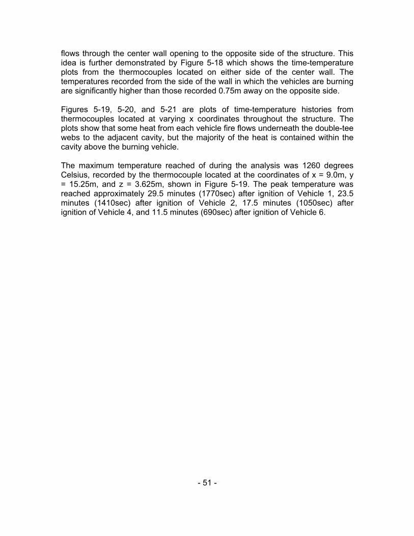
flows through the center wall opening to the opposite side of the structure. This idea is further demonstrated by Figure 5-18 which shows the time-temperature plots from the thermocouples located on either side of the center wall. The temperatures recorded from the side of the wall in which the vehicles are burning are significantly higher than those recorded 0.75m away on the opposite side. Figures 5-19, 5-20, and 5-21 are plots of time-temperature histories from thermocouples located at varying x coordinates throughout the structure. The plots show that some heat from each vehicle fire flows underneath the double-tee webs to the adjacent cavity, but the majority of the heat is contained within the cavity above the burning vehicle. The maximum temperature reached of during the analysis was 1260 degrees Celsius, recorded by the thermocouple located at the coordinates of x = 9.0m, y = 15.25m, and z = 3.625m, shown in Figure 5-19. The peak temperature was reached approximately 29.5 minutes (1770sec) after ignition of Vehicle 1, 23.5 minutes (1410sec) after ignition of Vehicle 2, 17.5 minutes (1050sec) after ignition of Vehicle 4, and 11.5 minutes (690sec) after ignition of Vehicle 6.

- 52 -

12 4 3 56 7

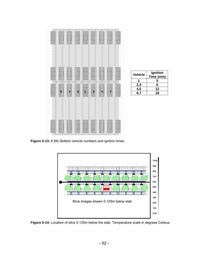
Figure 5-13: 6 Min Bottom vehicle numbers and ignition times.


Vehicle Ignition Time (min)

1 0 2,3 6 4,5 12 6,7 18

Slice images shown 0.125m below slabSlice images shown 0.125m below slab Slice images shown 0.125m below slab

- 53 -

Figure 5-15: 6 Min Bottom slice images showing temperature distribution throughout the structure.

6 Minutes

12 Minutes

18 Minutes

- 54 -


24 Minutes

30 Minutes

36 Minutes

- 55 -


42 Minutes

48 Minutes

54 Minutes

- 56 -


60 Minutes

66 Minutes

72 Minutes

- 57 -


78 Minutes

84 Minutes

90 Minutes

- 58 -

Figure 5-15: 6 Min Bottom slice image (continued) .

0100200300400500600700800900

100011001200130014001500

0 1200 2400 3600 4800

Time (sec)

Tem

pera

ture

(deg

. C)

y = 0.25my = 9.0my = 18.0my = 15.25m


96 Minutes

y = 0.25m y = 9.0m

y = 15.25m

y = 18.0m

- 59 -

0100200300400500600700800900

100011001200130014001500

0 1200 2400 3600 4800

Time (sec)

Tem

pera

ture

(deg

. C)

y = 18.75my = 21.0my = 36.25my = 27.5


0100200300400500600700800900

100011001200130014001500

0 1200 2400 3600 4800

Time (sec)

Tem

pera

ture

(deg

. C)

y = 18.0m

y = 18.75m


y = 18.75m y = 21.0m

y = 27.5m y = 36.25m

y = 18.0m y = 18.75m

- 60 -

0100200300400500600700800900

100011001200130014001500

0 1200 2400 3600 4800

Time (sec)

Tem

pera

ture

(deg

. C)

x = 11.25m

x = 9.0m

x = 6.75m


0100200300400500600700800900

100011001200130014001500

0 1200 2400 3600 4800

Time (sec)

Tem

pera

ture

(deg

. C)

x = 11.25mx = 9.0mx = 6.75m


x = 11.25m x = 9.0m x = 6.75m

x = 11.25m x = 9.0m x = 6.75m

- 61 -

0100200300400500600700800900

100011001200130014001500

0 1200 2400 3600 4800

Time (sec)

Tem

pera

ture

(deg

. C)

x = 11.25m

x = 9.0m

x = 6.75m


x = 11.25m x = 9.0m x = 6.75m

- 62 -

5.2.3 6 Min Top Analysis The geometry of the 6 Min Top model is similar to that of the 6 Min Bottom model, except that the top of the center wall opening position is flush with the bottom of the double-tee flange, as shown in Figure 5-22. The purpose of 6 Min Top was to investigate the effects varying the opening position of the center wall had on heat transfer throughout the structure. The material properties and analysis parameters of 6 Min Top were identical to those of 6 Min Bottom, with a 6 minute time interval between ignitions of adjacent vehicles. Slice images created using Smokeview are shown in Figure 5-23. The images display the temperature distribution through the structure 0.125m below the slab (Figure 5-22). As before, images were captured in 6 minute intervals and were recorded for the entire duration of the analysis. Unlike the previous two analyses, the images of Figure 5-23 show heat flowing freely through the center wall opening position to the other side of the structure. Time-temperature histories recorded by thermocouples throughout the structure are plotted in Figures 5-24 to 5-29. Longitudinal time-temperature plots are shown in Figures 5-24 to 5-26 and transverse time-temperature plots are shown in Figures 5-27 to 5-29. The maximum temperature reached during the analysis was 1503 degrees Celsius, recorded by the thermocouple located at x = 9.0m, y = 15.25m, and z = 3.625m, in the cavity above burning Vehicle 2. Figure 5-26 shows the time-temperature curves at locations on each side of the center wall. Very little difference is noticed between the two plots showing that the heat from the burning vehicles is freely transmitted through the wall opening to the other side of the garage.

- 63 -

Slice images shown 0.125m below slabSlice images shown 0.125m below slab


Slice images shown 0.125m below slab

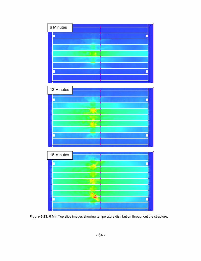
- 64 -

Figure 5-23: 6 Min Top slice images showing temperature distribution throughout the structure.

6 Minutes

12 Minutes

18 Minutes

- 65 -

Figure 5-23: 6 Min Top slice images (continued).

24 Minutes

30 Minutes

36 Minutes

- 66 -


42 Minutes

48 Minutes

54 Minutes

- 67 -


60 Minutes

66 Minutes

72 Minutes

- 68 -


78 Minutes

84 Minutes

90 Minutes

- 69 -

Figure 5-23: 6 Min Top slice image (continued).

0100200300400500600700800900

100011001200130014001500

0 1200 2400 3600 4800

Time (sec)

Tem

pera

ture

(deg

. C)

y = 0.25my = 9.0my = 18.0my = 15.25m

Figure 5-24: 6 Min Top time-temperature histories centered between double-tee webs above burning vehicle at x = 11.25m; y = 0.25m, 9.0m, 15.25m, 18.0m; z = 3.625m.

96 Minutes

y = 0.25m y = 9.0m

y = 15.25m

y = 18.0m

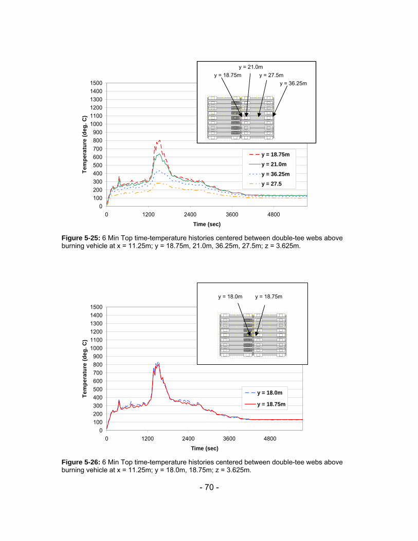
- 70 -

0100200300400500600700800900

100011001200130014001500

0 1200 2400 3600 4800

Time (sec)

Tem

pera

ture

(deg

. C)

y = 18.75my = 21.0my = 36.25my = 27.5

Figure 5-25: 6 Min Top time-temperature histories centered between double-tee webs above burning vehicle at x = 11.25m; y = 18.75m, 21.0m, 36.25m, 27.5m; z = 3.625m.

0100200300400500600700800900

100011001200130014001500

0 1200 2400 3600 4800

Time (sec)

Tem

pera

ture

(deg

. C)

y = 18.0m

y = 18.75m

Figure 5-26: 6 Min Top time-temperature histories centered between double-tee webs above burning vehicle at x = 11.25m; y = 18.0m, 18.75m; z = 3.625m.

y = 18.75m y = 21.0m

y = 27.5m y = 36.25m

y = 18.0m y = 18.75m

- 71 -

0100200300400500600700800900

100011001200130014001500

0 1200 2400 3600 4800

Time (sec)

Tem

pera

ture

(deg

. C)

x = 11.25m

x = 9.0m

x = 6.75m

Figure 5-27: 6 Min Top time-temperature histories centered between double-tee webs above burning vehicle at x = 11.25m, 9.0m, 6.75m; y = 15.25m; z = 3.625m.

0100200300400500600700800900

100011001200130014001500

0 1200 2400 3600 4800

Time (sec)

Tem

pera

ture

(deg

. C)

x = 11.25mx = 9.0mx = 6.75m


x = 11.25m x = 9.0m x = 6.75m

x = 11.25m x = 9.0m x = 6.75m

- 72 -

0100200300400500600700800900

100011001200130014001500

0 1200 2400 3600 4800

Time (sec)

Tem

pera

ture

(deg

. C)

x = 11.25mx = 9.0mx = 6.75m


x = 11.25m x = 9.0m x = 6.75m

- 73 -

CHAPTER 6

DISCUSSION OF FIRE ANALYSIS RESULTS This chapter discusses the results of the FDS analyses presented in Chapter 5. Section 6.1 compares the results of 12 Min Bottom and 6 Min Bottom, and investigates the effects a shorter time interval between ignitions of adjacent vehicles has on the gas temperatures recorded throughout the structure. Section 6.2 compares the results of 6 Min Bottom and 6 Min Top and addresses the influence center wall opening position has on gas temperatures and heat transmission throughout the structure. 6.1 EFFECTS OF TIME INTERVAL BETWEEN IGNITIONS OF ADJACENT

VEHICLES ON HEAT TRANSMISSION In order to determine the effects the time interval between ignitions of adjacent vehicles had on the gas temperatures recorded in the double-tee web cavities, the results of 12 Min Bottom and 6 Min Bottom were compared. The geometry of the model in each analysis was identical, the same material properties were used, and the same FDS heat release rate input was used for each analysis. The only parameter that varied between the two analyses was the elapsed period of time between ignition of each vehicle and the adjacent one. In 12 Min Bottom, Vehicle 1 ignited at T = 0, Vehicles 2 and 3 ignited at ΔT = +12 minutes, Vehicles 4 and 5 at ΔT = +24 minutes, and Vehicles 6 and 7 at ΔT = +36 minutes. In 6 Min Bottom, the time periods were halved, resulting in Vehicles 2 and 3 igniting at ΔT = +6 minutes, Vehicles 4 and 5 at ΔT = +12 minutes, and Vehicles 6 and 7 at ΔT = +18 minutes. Consistent with 12 Min Bottom, Vehicle 1 ignited at T = 0. Because the geometry of the model and burning sequences for each analysis were symmetric about Vehicle 1, data collected from the thermocouples on the left side of Vehicle 1 was analyzed (Figure 6-1). Figures 6-2 and 6-3 show the gas time temperature histories for thermocouples located along the length of the double-tee flange located above burning Vehicle 1. Comparing the figures, it is evident that the temperatures recorded at each set of coordinates were significantly greater in 6 Min Bottom. The maximum gas temperature reached in 6 Min Bottom was more than 300 degrees greater than the maximum temperature reached in 12 Min Bottom. Figures 6-4 and 6-5 show the time temperature histories for thermocouples located along the x-axis in the double-tee web cavities above the burning vehicles in 12 Min Bottom and 6 Min Bottom. Comparing the figures from each

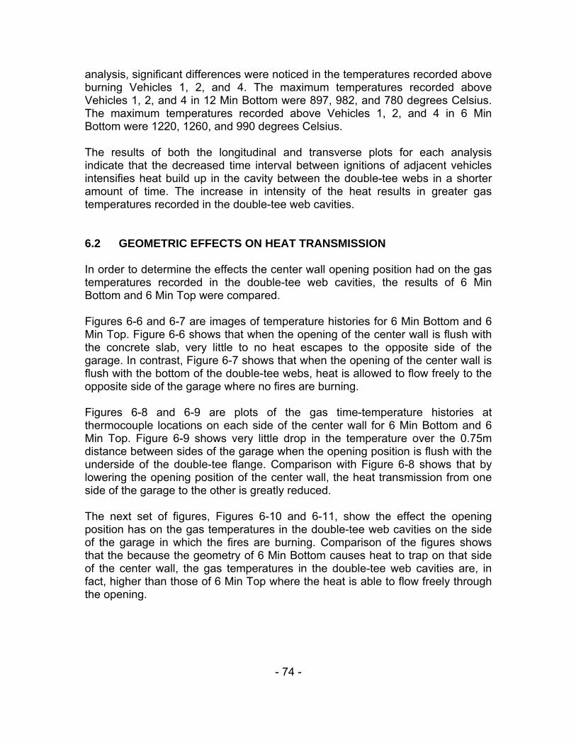
- 74 -

analysis, significant differences were noticed in the temperatures recorded above burning Vehicles 1, 2, and 4. The maximum temperatures recorded above Vehicles 1, 2, and 4 in 12 Min Bottom were 897, 982, and 780 degrees Celsius. The maximum temperatures recorded above Vehicles 1, 2, and 4 in 6 Min Bottom were 1220, 1260, and 990 degrees Celsius. The results of both the longitudinal and transverse plots for each analysis indicate that the decreased time interval between ignitions of adjacent vehicles intensifies heat build up in the cavity between the double-tee webs in a shorter amount of time. The increase in intensity of the heat results in greater gas temperatures recorded in the double-tee web cavities. 6.2 GEOMETRIC EFFECTS ON HEAT TRANSMISSION In order to determine the effects the center wall opening position had on the gas temperatures recorded in the double-tee web cavities, the results of 6 Min Bottom and 6 Min Top were compared. Figures 6-6 and 6-7 are images of temperature histories for 6 Min Bottom and 6 Min Top. Figure 6-6 shows that when the opening of the center wall is flush with the concrete slab, very little to no heat escapes to the opposite side of the garage. In contrast, Figure 6-7 shows that when the opening of the center wall is flush with the bottom of the double-tee webs, heat is allowed to flow freely to the opposite side of the garage where no fires are burning. Figures 6-8 and 6-9 are plots of the gas time-temperature histories at thermocouple locations on each side of the center wall for 6 Min Bottom and 6 Min Top. Figure 6-9 shows very little drop in the temperature over the 0.75m distance between sides of the garage when the opening position is flush with the underside of the double-tee flange. Comparison with Figure 6-8 shows that by lowering the opening position of the center wall, the heat transmission from one side of the garage to the other is greatly reduced. The next set of figures, Figures 6-10 and 6-11, show the effect the opening position has on the gas temperatures in the double-tee web cavities on the side of the garage in which the fires are burning. Comparison of the figures shows that the because the geometry of 6 Min Bottom causes heat to trap on that side of the center wall, the gas temperatures in the double-tee web cavities are, in fact, higher than those of 6 Min Top where the heat is able to flow freely through the opening.

- 75 -

Figure 6-1: Location of thermocouples.

- 76 -

0100200300400500600700800900

100011001200130014001500

0 1200 2400 3600 4800

Time (sec)

Tem

pera

ture

(deg

. C)

y = 0.25my = 9.0my = 18.0my = 15.25m


0100200300400500600700800900

100011001200130014001500

0 1200 2400 3600 4800

Time (sec)

Tem

pera

ture

(deg

. C)

y = 0.25my = 9.0my = 18.0my = 15.25m


- 77 -

0100200300400500600700800900

100011001200130014001500

0 1200 2400 3600 4800

Time (sec)

Tem

pera

ture

(deg

. C)

x = 11.25m

x = 9.0m

x = 6.75m


0100200300400500600700800900

100011001200130014001500

0 1200 2400 3600 4800

Time (sec)

Tem

pera

ture

(deg

. C)

x = 11.25m

x = 9.0m

x = 6.75m


- 78 -

Figure 6-6: Slice image for 6 Min Bottom showing temperature distribution 0.125m below slab above burning vehicles.

Figure 6-7: Slice image for 6 Min Top showing temperature distribution 0.125m below slab above burning vehicles.

30 Minutes

30 Minutes

- 79 -

0100200300400500600700800900

100011001200130014001500

0 1200 2400 3600 4800

Time (sec)

Tem

pera

ture

(deg

. C)

y = 18.0m

y = 18.75m


0100200300400500600700800900

100011001200130014001500

0 1200 2400 3600 4800

Time (sec)

Tem

pera

ture

(deg

. C)

y = 18.0m

y = 18.75m

Figure 6-9: 6 Min Top time-temperature histories centered between double-tee webs above burning vehicle at x = 11.25m; y = 18.0m, 18.75m; z = 3.625m.

- 80 -

0100200300400500600700800900

100011001200130014001500

0 1200 2400 3600 4800

Time (sec)

Tem

pera

ture

(deg

. C)

x = 11.25mx = 9.0mx = 6.75m


0100200300400500600700800900

100011001200130014001500

0 1200 2400 3600 4800

Time (sec)

Tem

pera

ture

(deg

. C)

x = 11.25mx = 9.0mx = 6.75m


- 81 -

CHAPTER 7

NON-LINEAR HEAT TRANSFER ANALYSIS

As discussed in Chapter 4, the fire analyses were conducted as follows: Models were constructed using a graphical interface (PyroSim). The program then generated a text file containing the input parameters needed to run the fire analyses. Those text files were run using the FDS program, and, upon completion, two types of output data were written to files. The first type of FDS output data was presented in Chapter 5 in the form of time-temperature plots and slice file images for each analysis. This chapter explains the use of the second type of FDS output data, mainly the heat flux time histories. Section 7.1 begins with a description of the non-linear heat transfer analysis procedure used to obtain concrete temperatures throughout the structure. Section 7.1.1 describes the FDS model, while Section 7.1.2 describes the finite element model. For each of the three analysis cases, the temperatures at the level of the prestressing strands in the double-tee webs were determined. The results of the strand level temperatures for each of the individual analysis cases (12 Min Bottom, 6 Min Bottom, and 6 Min Top) are presented in Section 7.2. Temperatures along the surface of the double-tees were also determined and are discussed in Chapter 8. 7.1 NON-LINEAR HEAT TRANSFER ANALYSIS PROCEDURE As was shown in Chapter 5, the gas time-temperature histories obtained from the first type of FDS output data were very useful for comparing analyses. However, when investigating the effects of vehicle fires on concrete structures, the temperature distribution within the structural member itself should also be examined in order to fully understand the implications fire loading has on the structural integrity of the member. In order to determine the temperature distribution within the structural member, the heat flux time histories were utilized to conduct a non-linear heat transfer analysis. The goal of the heat transfer analysis was to obtain the temperature distribution at key locations of the structure, specifically the temperatures at the levels of the prestressing strands and on the surface of the flange above the stems. The first step in completing the heat transfer analysis involved the use of the second type of FDS output files, the Boundary Files. As mentioned in Chapter 4, Boundary Files were used to gather heat flux data in 30 second increments throughout the duration of the analysis. In order to be usable as input to the finite

- 82 -

element model, the heat flux output files first had to be converted to text files using a computer program. The program, called FDS2ascii, is a Fortran 90 program that was written at NIST and is a user interactive program that returns heat flux values in text files upon answering specific parameter questions. The returned heat flux values are then used as the input into the finite element analysis. 7.1.1 FDS Model Because this research was intended to draw comparisons with an analysis previously described in Bayreuther (2006), the procedure followed to create an input file for the finite element analysis remained unchanged. The following explanation, describing the process of creating an input file for the finite element analysis, was extracted from Bayreuther (2006). Figure 7-1 shows the FDS double-tee model with specific nodes labeled. For the model used in this project, the web of the double-tee is modeled as explained previously with cubic elements with a side length of 0.125m. The slab is one element thick and the web is six elements deep by two elements wide. The FDS net heat flux outputs are recorded at seven nodes (labeled A-G) on the web of the double-tees. To create an input file for the finite element analysis, the nodal heat flux values on each surface are averaged to get a uniform net heat flux for each of the surfaces 1 through 5 (Figure 7-2). Because the goal of the heat transfer analysis was to estimate the heat distribution throughout the double-tee web, the heat flux data was gathered at nodes on the web itself. Upon further investigation, it was determined that the net heat flux on any specific surface on the model was essentially uniform, which enabled the nodal heat flux values on each surface to be averaged and used as the finite element model input. Figures 7-3 to 7-5 show the uniform trends of the heat flux recorded at each node on a specific surface. 7.1.2 Finite Element Model Again, for consistency purposes, the finite element model remained unchanged from that of Bayreuther (2006). The following section from Bayreuther (2006) describes the details of the model. The non-linear finite element transient heat transfer analysis used in this project for purposes of results analysis was performed using the ABAQUS non-linear finite elements software package. A model of the double-tee web was

- 83 -

constructed based on the procedures explained in Okasha (2006). The following section provides details of the model. A three-dimensional unit-thickness slice of a double-tee web was constructed based on the dimensions of the 15DT34 double-tee from the PCI handbook and the 188-S strand pattern (18 strands of 8/16 inch diameter). The element type was a solid (continuum), first order (eight nodes), hexahedra (brick) element called DC3D8 in ABAQUS with full integration. The element mesh configuration is eight elements across the web and four elements through the thickness of the slab. The mesh is finer than the configuration used in Okasha, which was four elements across the web and three through the slab thickness and was based on a convergence study for accuracy. The trend from the convergence study was that the finer mesh with similar element aspect ratio resulted in higher accuracy. Therefore the configuration used for this project is at least as accurate as that used for Okasha (2006). The element mesh configuration provides nodes located at the levels of the prestressing strands in the web. This allows nodal temperatures to be calculated directly and used to analyze the potential changes to the steel strength because of elevated temperatures. Figure 7-6 shows an elevation view of the finite element model with dimensions, elements, and strand level labeling shown. The difference between the heat transfer analysis in Okasha and this project is the load input. Okasha uses the standard ASTM E119 time-temperature curve as the load, while this project uses the net heat flux output as previously described. In this case, the net heat transfer averages from FDS for the five surfaces in the model are defined as field inputs for the finite element model. All other parameters are the same, including material and environmental properties, which are identical to those explained in Section 4.2.1. 7.2 INDIVIDUAL NON-LINEAR HEAT TRANSFER ANALYSIS RESULTS The following sections present the results of each of the individual analyses. For each analysis, the temperatures at the levels of the prestressing strands in three of the double-tee webs were obtained. The double-tee webs of interest will be referred to as Webs 3, 4, and 5, and are shown in Figure 7-7. 7.2.1 12 Min Bottom The concrete time-temperature curves for Webs 3, 4, and 5 for 12 Min Bottom are shown in Figures 7-8, 7-9, and 7-10, respectively. As expected, the maximum temperatures computed are at the lowest strand level (Strand Level 1), which is

- 84 -

44.6mm from the bottom of the web. The highest temperatures at Strand Level 1 for Webs 3, 4, and 5, were 141, 173, and 214 degrees Celsius, respectively. 7.2.2 6 Min Bottom The concrete time-temperature curves for Webs 3, 4, and 5 for 6 Min Bottom are shown in Figures 7-11, 7-12, and 7-13. Again, the maximum temperature was computed at Strand Level 1 in each web. The highest temperatures at Strand Level 1 for Webs 3, 4, and 5, were 204, 230, and 249 degrees Celsius, respectively. 7.2.3 6 Min Top The concrete time-temperature curves for Webs 3, 4, and 5 for 6 Min Top are shown in Figures 7-14, 7-15, and 7-16. Again, the maximum temperature was computed at Strand Level 1 in each web. The highest temperatures at Strand Level 1 for Webs 3, 4, and 5, were 205, 236, and 238 degrees Celsius, respectively.

- 85 -

A

B

CDE

F

G

FDS Node Labeling

x

y

A

B

CDE

F

G

FDS Node Labeling

A

B

CDE

F

G A

B

CDE

F

G

FDS Node Labeling

x

y

Figure 7-1: FDS double-tee model with node labeling.

A

B

CDE

F

G

1

4

2

3

5

FDS Node Labeling FDS Surface Labeling

x

y

A

B

CDE

F

G

1

4

2

3

5


A

B

CDE

F

G A

B

CDE

F

G

1

4

2

3

5

1

4

2

3

5


x

y

Figure 7-2: FDS double-tee model for heat flux averages with nodes labeled (left) and surfaces labeled (right).

- 86 -

0

10

20

30

40

50

60

70

0 600 1200 1800 2400 3000 3600 4200 4800 5400

Time (sec)

Net

Hea

t Flu

x (k

W/m

2)

Ax

Bx

Cx

Figure 7-3: Heat flux on Surface 1 for 6 Min Bottom.

0

10

20

30

40

50

60

70

0 600 1200 1800 2400 3000 3600 4200 4800 5400

Time (sec)

Net

Hea

t Flu

x (k

W/m

2)

Cy

Dy

Ey


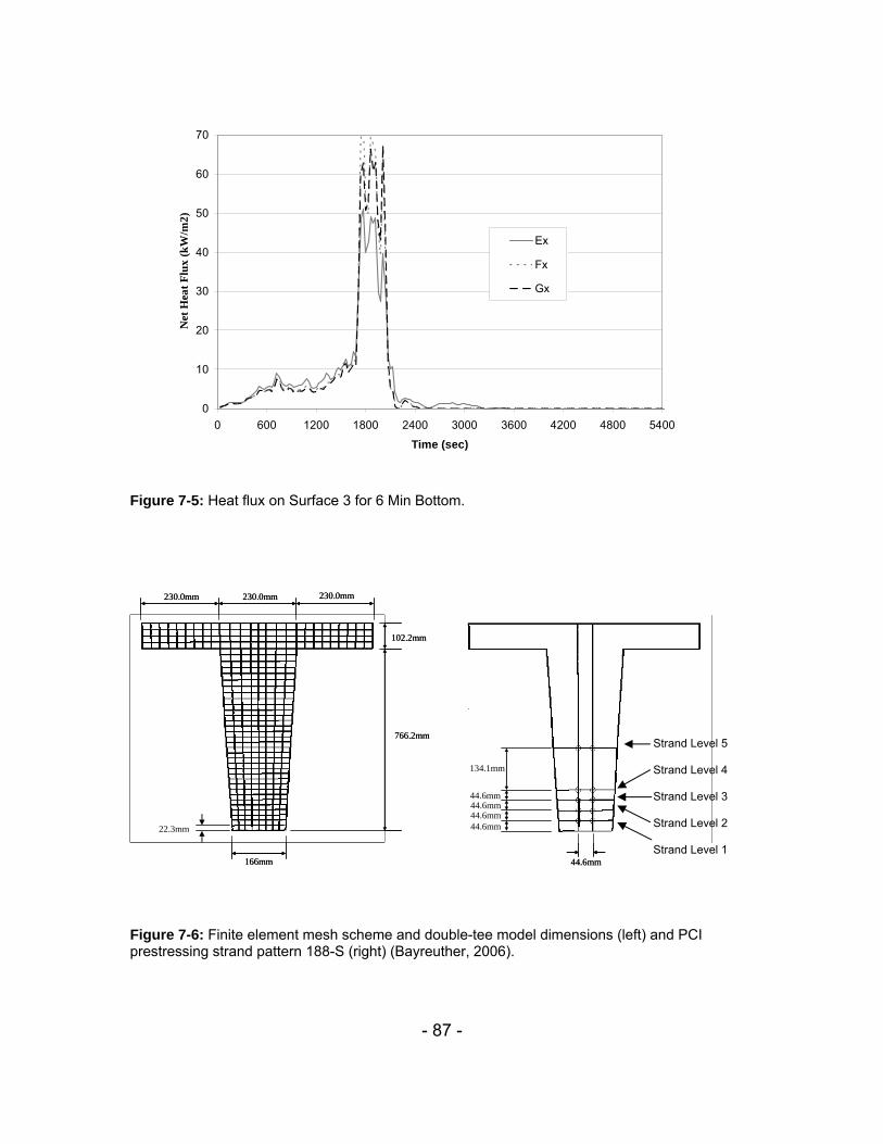
- 87 -

0

10

20

30

40

50

60

70

0 600 1200 1800 2400 3000 3600 4200 4800 5400

Time (sec)

Net

Hea

t Flu

x (k

W/m

2)

Ex

Fx

Gx


Figure 7-6: Finite element mesh scheme and double-tee model dimensions (left) and PCI prestressing strand pattern 188-S (right) (Bayreuther, 2006).

766.2mm

22.3mm

166mm

230.0mm230.0mm230.0mm

102.2mm

134.1mm

44.6mm44.6mm44.6mm44.6mm

44.6mm

766.2mm

22.3mm

166mm

230.0mm230.0mm230.0mm

102.2mm

134.1mm

44.6mm44.6mm44.6mm44.6mm

44.6mm

Strand Level 5 Strand Level 4 Strand Level 3 Strand Level 2 Strand Level 1

- 88 -

Figure 7-7: Labeling of double-tee webs.

0

40

80

120

160

200

240

280

0 2000 4000 6000 8000 10000

Time (s)

Tem

pera

ture

(deg

C)

Strand Level 1Strand Level 2Strand Level 3Strand Level 4Strand Level 5

Figure 7-8: 12 Min Bottom time-temperature curves at the levels of the prestressing strands of Web 3.

Web 5

Web 4

Web 3

- 89 -

0

40

80

120

160

200

240

280

0 2000 4000 6000 8000 10000

Time (s)

Tem

pera

ture

(deg

C)


Figure 7-9: 12 Min Bottom time-temperature curves for at the levels of the prestressing strands of Web 4.

0

40

80

120

160

200

240

280

0 2000 4000 6000 8000 10000

Time (s)

Tem

pera

ture

(deg

C)



- 90 -

0

40

80

120

160

200

240

280

0 2000 4000 6000 8000 10000

Time (s)

Tem

pera

ture

(deg

C)



0

40

80

120

160

200

240

280

0 2000 4000 6000 8000 10000

Time (s)

Tem

pera

ture

(deg

C)



- 91 -

0

40

80

120

160

200

240

280

0 2000 4000 6000 8000 10000

Time (s)

Tem

pera

ture

(deg

C)



0

40

80

120

160

200

240

280

0 2000 4000 6000 8000 10000

Time (s)

Tem

pera

ture

(deg

C)

Strand Level 1

Strand Level 2

Strand Level 3

Strand Level 4

Strand Level 5

Figure 7-14: 6 Min Top time-temperature curves at the levels of the prestressing strands of Web 3.

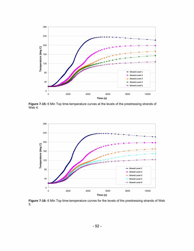
- 92 -

0

40

80

120

160

200

240

280

0 2000 4000 6000 8000 10000

Time (s)

Tem

pera

ture

(deg

C)

Strand Level 1

Strand Level 2

Strand Level 3

Strand Level 4

Strand Level 5

Figure 7-15: 6 Min Top time-temperature curves at the levels of the prestressing strands of Web 4.

0

40

80

120

160

200

240

280

0 2000 4000 6000 8000 10000

Time (s)

Tem

pera

ture

(deg

C)

Strand Level 1

Strand Level 2

Strand Level 3

Strand Level 4

Strand Level 5

Figure 7-16: 6 Min Top time-temperature curves for the levels of the prestressing strands of Web 5.

- 93 -

CHAPTER 8

DISCUSSION OF NON-LINEAR HEAT TRANSFER RESULTS

This chapter explains the results of the non-linear heat transfer analyses presented in Chapter 7. Section 8.1 compares the results of 12 Min Bottom and 6 Min Bottom, and investigates the time interval between ignitions of adjacent vehicles has on the concrete temperatures at the level of the first prestressing strand of the double-tee webs. Section 8.2 compares the results of 6 Min Bottom and 6 Min Top and examines the effects of center wall opening position on the concrete temperatures. Section 8.3 discusses the implications of these results on structural design. Section 8.4 presents a discussion of flange surface temperatures obtained from the finite element analyses, and Section 8.5 follows with a discussion of the implications of these results with respect to ASTM E 119 criteria. 8.1 EFFECTS OF TIME INTERVAL BETWEEN IGNITIONS OF ADJACENT

VEHICLES ON PRESTRESSING STRAND TEMPERATURES In order to determine the effects a shorter time duration between ignitions of adjacent vehicles has on the temperature at the locations of the prestressing strands of the double-tee webs, the results of the non-linear heat transfer analyses of 12 Min Bottom and 6 Min Bottom were compared. As shown in Figure 8-1 (12 Min Bottom Web 5 and 6 Min Bottom Web 5), the concrete time-temperature curve for 12 Min Bottom is significantly lower than that of 6 Min Bottom. The data indicates that shorter time durations between ignitions of adjacent vehicles in a multi-vehicle fire analysis causes in an increase of heat flux into the structure, resulting in higher concrete temperatures. In order to fully understand the causes of this result, time-heat flux plots from each Analysis were studied. Figure 8-2 displays time-heat flux data from Surface 1 of double-tee Web 5 for each analysis. The curve from 6 Min Bottom shows a noticeable spike in the heat flux value occurring approximately 360 seconds into the analysis. A peak is evident at that time in 12 Min Bottom as well; however the value is more than three times less than that of 6 Min Bottom. Upon further investigation, this trend is again apparent from 1350 seconds to 1800 seconds. The maximum heat flux value obtained in 6 Min Bottom between those times is 62 kW/m2, while the maximum heat flux value obtained in 12 Min Bottom was only 30 kW/m2. The consistently higher energy release rates obtained over time in 6 Min Bottom result in the increased concrete temperatures that were shown in Figure 8-1.

- 94 -

8.2 EFFECTS OF CENTER WALL OPENING POSITION ON CONCRETE TEMPERATURE

In order to determine the effects the center wall opening position had on the temperature at the locations of the prestressing strands of the double-tee webs, the results of the non-linear heat transfer analyses of 6 Min Bottom and 6 Min Top were compared. In each analysis, maximum strand level temperatures occurred at the first strand level of Web 5 (above burning Vehicle 1). Figure 8-3 (6 min Bottom and 6 min Top) shows the plots of the time-temperature data from each analysis. Comparing the plots, the temperatures in 6 Min Bottom are higher than those of 6 Min Top. As was discussed in Chapter 6, the bottom opening center wall position traps the heat on one side of the garage, thus, increasing the intensity of heat on that side. The increased heat flux values (Figure 8-2) consequently result in greater temperatures at the strand levels. In contrast, in 6 Min Top, when heat is allowed to freely flow to the opposite side of the garage, a decrease in the heat flux becomes evident, resulting in lower strand level temperatures. 8.3 REDUCTION IN PRESTRESSING STEEL STRENGTH The main objective of the non-linear heat transfer analysis described in Chapter 7 was to determine the concrete temperature at the levels of the prestressing strands of the double-tee webs above the burning vehicles. The results of each of these analyses were presented in Section 7.2. As was shown in Section 7.2, the maximum strand level temperatures achieved during each analysis were recorded in Web 5 (above burning Vehicle 1) at the first level of prestressing strands. In order to determine the impact this fire loading had on the structure, calculations to determine the reduction in strength in the prestressing steel were completed following the Eurocode 1. Table 8-1 presents a summary of the maximum strand temperatures obtained and the percent of strength reduction in prestressing strands for each analysis. The maximum temperature obtained in any model was 249 degrees Celsius, recorded in 6 Min Bottom above burning Vehicle 1. At 249 degrees Celsius, the strength reduction of the prestressing steel is approximately 20%. The maximum temperature obtained in 12 Min Bottom was 214 degrees Celsius, which results in a 15% reduction in strength. Finally, the maximum temperature obtained in 6 Min Top was 238 degrees Celsius, which results in a 19% reduction in strength. Figure 8-4 shows a graph of the temperature dependent stress-strain curves for the prestressing steel.

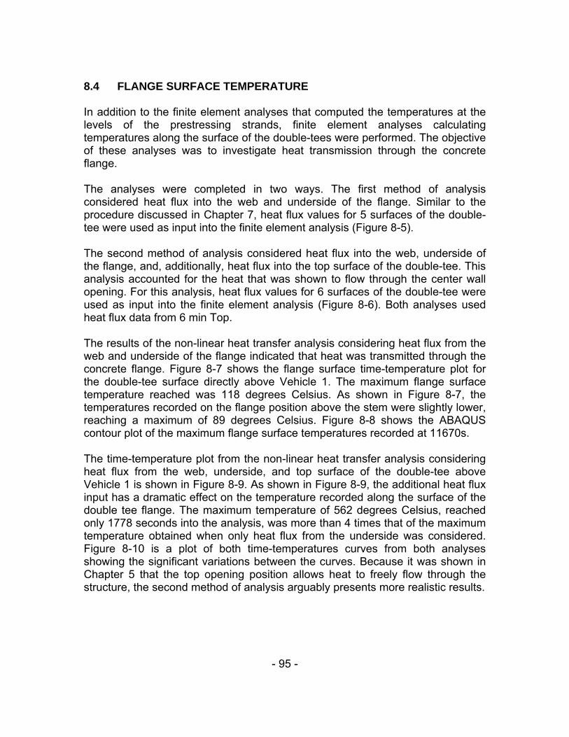
- 95 -

8.4 FLANGE SURFACE TEMPERATURE In addition to the finite element analyses that computed the temperatures at the levels of the prestressing strands, finite element analyses calculating temperatures along the surface of the double-tees were performed. The objective of these analyses was to investigate heat transmission through the concrete flange. The analyses were completed in two ways. The first method of analysis considered heat flux into the web and underside of the flange. Similar to the procedure discussed in Chapter 7, heat flux values for 5 surfaces of the double-tee were used as input into the finite element analysis (Figure 8-5). The second method of analysis considered heat flux into the web, underside of the flange, and, additionally, heat flux into the top surface of the double-tee. This analysis accounted for the heat that was shown to flow through the center wall opening. For this analysis, heat flux values for 6 surfaces of the double-tee were used as input into the finite element analysis (Figure 8-6). Both analyses used heat flux data from 6 min Top. The results of the non-linear heat transfer analysis considering heat flux from the web and underside of the flange indicated that heat was transmitted through the concrete flange. Figure 8-7 shows the flange surface time-temperature plot for the double-tee surface directly above Vehicle 1. The maximum flange surface temperature reached was 118 degrees Celsius. As shown in Figure 8-7, the temperatures recorded on the flange position above the stem were slightly lower, reaching a maximum of 89 degrees Celsius. Figure 8-8 shows the ABAQUS contour plot of the maximum flange surface temperatures recorded at 11670s. The time-temperature plot from the non-linear heat transfer analysis considering heat flux from the web, underside, and top surface of the double-tee above Vehicle 1 is shown in Figure 8-9. As shown in Figure 8-9, the additional heat flux input has a dramatic effect on the temperature recorded along the surface of the double tee flange. The maximum temperature of 562 degrees Celsius, reached only 1778 seconds into the analysis, was more than 4 times that of the maximum temperature obtained when only heat flux from the underside was considered. Figure 8-10 is a plot of both time-temperatures curves from both analyses showing the significant variations between the curves. Because it was shown in Chapter 5 that the top opening position allows heat to freely flow through the structure, the second method of analysis arguably presents more realistic results.

- 96 -

8.5 IMPLICATIONS OF SURFACE TEMPERATURE RESULTS WITH RESPECT TO ASTM E 119 HEAT TRANSMISSION CRITERIA

As was discussed in Section 2.3, the ASTM E 119 tests include end point criteria. The capacity of the structural member to limit the heat transfer from the exposed side to the unexposed side is addressed by the criterion as follows: The temperature increase of the unexposed surface must not exceed an average of 250 degrees Fahrenheit (121.1 degrees Celsius), or a maximum of 325 degrees Fahrenheit (162.7 degrees Celsius) at any one point. In most jurisdictions, concrete slabs requiring a fire-resistance rating (such as those used in the construction of parking structures) must satisfy this heat transmission requirement. As was explained in Section 8.4, the finite element analysis that was conducted using heat flux inputs from only the underside of the double-tee resulted in average flange surface temperatures less than the prescribed temperature of 121 degrees Celsius, and well below the prescribed maximum of temperature of 162.7 degrees Celsius (Figure 8-6). However, when the finite element analysis considering an additional heat flux due to heat transmission through the center wall opening was conducted, the results indicated flange surface temperatures well above the prescribed maximum values. The maximum temperature obtained in the analysis was 562 degrees Celsius, nearly 200 degrees greater than that of the prescribed value. These results suggest that, when designing for fire resistance, structural members of precast concrete parking structures similar to the structure treated in this study should not necessarily have to adhere to the heat transmission requirements prescribed by the standard ASTM E 119 tests because heat from the burning vehicle(s) is not only going to heat the underside of the double-tee, but will also flow through the center wall opening, thus heating the flange surface and causing a temperature increase well above the prescribed maximum. The results indicate that it is not necessary to be concerned with through transmission criteria because both surfaces of the flange are going to be heated anyway.

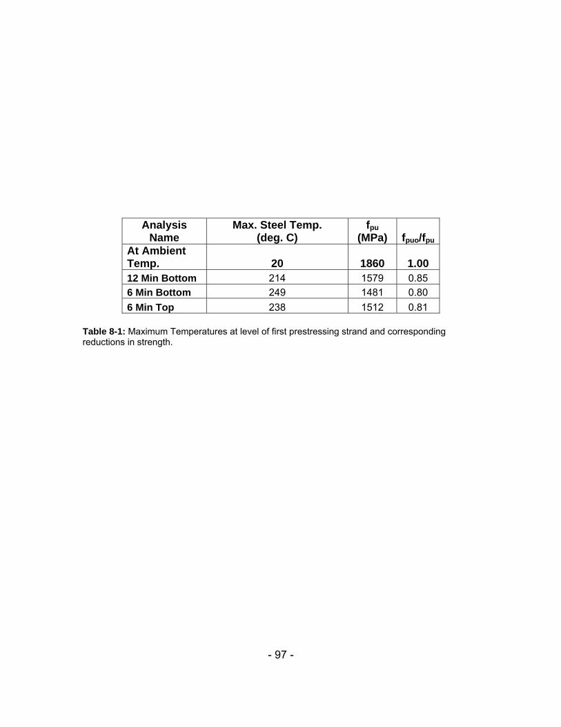
- 97 -

Analysis Name

Max. Steel Temp. (deg. C)

fpu (MPa) fpuo/fpu

At Ambient Temp. 20 1860 1.00 12 Min Bottom 214 1579 0.85 6 Min Bottom 249 1481 0.80 6 Min Top 238 1512 0.81

Table 8-1: Maximum Temperatures at level of first prestressing strand and corresponding reductions in strength.

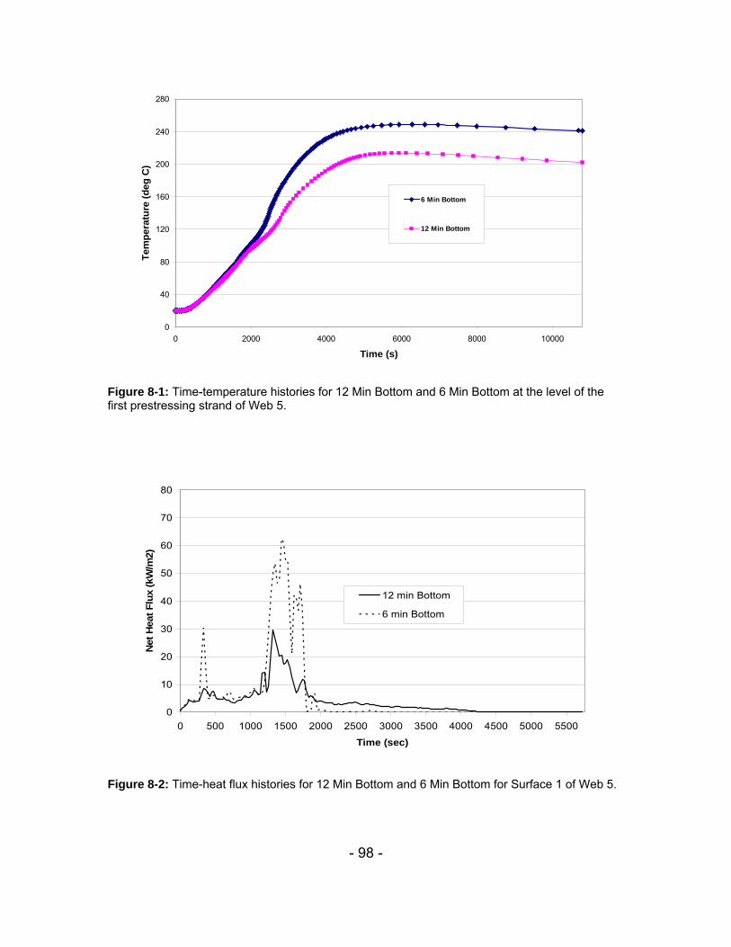
- 98 -

0

40

80

120

160

200

240

280

0 2000 4000 6000 8000 10000

Time (s)

Tem

pera

ture

(deg

C)

6 Min Bottom

12 Min Bottom

Figure 8-1: Time-temperature histories for 12 Min Bottom and 6 Min Bottom at the level of the first prestressing strand of Web 5.

0

10

20

30

40

50

60

70

80

0 500 1000 1500 2000 2500 3000 3500 4000 4500 5000 5500

Time (sec)

Net

Hea

t Flu

x (k

W/m

2)

12 min Bottom

6 min Bottom

Figure 8-2: Time-heat flux histories for 12 Min Bottom and 6 Min Bottom for Surface 1 of Web 5.

- 99 -

0

40

80

120

160

200

240

280

0 2000 4000 6000 8000 10000

Time (s)

Tem

pera

ture

(deg

C) Top Opening

Bottom Opening

Figure 8-3: Time-temperature histories for 6 Min Bottom and 6 Min Top at the level of the first prestressing strand of Web 5.

Figure 8-4: Temperature dependent stress-strain curves for prestressing steel.

0

200

400

600

800

1000

1200

1400

1600

1800

2000

0 0.005 0.01 0.015 0.02 0.025 0.03 0.035 0.04

Strain

Stre

ss (M

Pa)

214 deg. C (12 Min Bottom)

238 deg. C (6 Min Top)

249 deg. C (6 Min Bottom)

Ambient temp. = 20 deg. C

- 100 -

Surface 5

Surface 1

Surface 2

Surface 3

Surface 4Surface 5

Surface 1

Surface 2

Surface 3

Surface 4

Surface 5

Surface 1

Surface 2

Surface 3

Surface 4Surface 5

Surface 1

Surface 2

Surface 3

Surface 4

Additional Input – Surface 6

Figure 8-5: Surfaces 1-5 from which heat flux values were used as input to ABAQUS.

Figure 8-6: Surfaces 1-6 from which heat flux values were used as input to ABAQUS.

- 101 -

0

20

40

60

80

100

120

140

0 1000 2000 3000 4000 5000 6000 7000 8000 9000 10000

Time (sec)

Surf

ace

Tem

pera

ture

(deg

. C)

Flange surface

Surface above web

Average

Figure 8-7: Concrete temperatures on flange surface for 6 Min Top (heat flux input from web and underside only).

Figure 8-8: ABAQUS contour plot of concrete temperatures.

- 102 -

0

100

200

300

400

500

600

0 1000 2000 3000 4000 5000 6000 7000 8000 9000 10000

Time (s)

Tem

pera

ture

(deg

C)

Flange Surface

Flange position above stem

Figure 8-9: Concrete temperatures on flange surface for 6 Min Top (heat flux input from web, underside, and top surface).

0

100

200

300

400

500

600

0 1000 2000 3000 4000 5000 6000 7000 8000 9000 10000

Time (sec)

Surf

ace

Tem

pera

ture

(deg

. C)

Heat flux from web and underside

Heat flux from web, underside, and topsurface

Figure 8-10: Comparison of concrete temperatures on flange surface for 6 Min Top by heat flux from web and underside only; and heat flux from web, underside, and top surface.

- 103 -

CHAPTER 9

CONCLUSIONS AND FUTURE WORK

9.1 SUMMARY This report describes research which is part of a broader research program at Lehigh University directed towards the development of realistic fire loads for structures. This report focuses on fire loads for precast concrete parking structures. It is a continuation of previous work by Bayreuther (2006). A parking garage was chosen for study because of its simple repeating geometry, uniform non-combustible construction, well-controlled ventilation conditions, and relatively well-defined fuel loading. The study focused on the Campus Square parking garage on the Lehigh University campus. The structure is a commonly used precast, prestressed structural system comprised of mutli-story columns, double tee beams, inverted tee beams, and L-shaped spandrel beams. Three multiple vehicle fire scenarios were treated in this research. Analysis variables included the influence of the center wall opening position, and the time interval between ignition of successive vehicles, on the resulting fire load. Analysis computations were performed using the computer program, Fire Dynamics Simulator (FDS), a computational fluid dynamics program developed by the National Institute of Standards and Technology. 9.2 CONCLUSIONS The following conclusions are drawn from the work presented in this report:

(1) The time interval between ignitions of adjacent vehicles in a multi-vehicle analysis impacts the heat build-up throughout the structure. A shorter time interval between ignitions of adjacent vehicles was shown to greatly intensify heat build up in the cavity between double-tee webs.

(2) The variations in geometry of the structure were shown to have a significant impact on heat transmission. The position of the center wall opening in relation to the floor either trapped heat on one side of the structure or allowed free transmission to the other side.

(3) For the fire scenarios considered, vehicle fires cause the strength of the prestressing steel to vary from 0.85fpu to 0.80fpu.

(4) When designing for fire resistance, structural members of precast concrete parking structures similar to the structure treated in this

- 104 -

study should not necessarily have to adhere to the heat transmission requirements prescribed by the standard ASTM E 119 tests.

9.3 FUTURE WORK Additional work is needed to broaden and deepen the results of this study. For example, future analyses should consider structures with closed boundary conditions due to walls, and structures with multiple successive bays (i.e. larger footprints). In both cases, the heat generated by fire may not as freely disperse from the location of fire origin and thus lead to higher gas temperatures and heat fluxes.

- 105 -

REFERENCES

American Society for Testing and Materials (ASTM) “Standard Test Methods for Fire Tests of Building Construction and Materials.” ASTM E 119-05a. West Conshohocken, PA, 2005. Bayreuther, J., “Analytical Investigation of Fire Loads for Precast Concrete Parking Structures.” Master’s Thesis, Department of Civil and Environmental Engineering, Lehigh University, Bethlehem, PA, (2006). Buchanan, A.H., Structural Design for Fire Safety. John Wiley & Sons, New York, 2002, pp. 230-235. European Committee for Standardization Eurocode 1: Actions on Structures. British Standard, 2002. Fleming, R.P., “Assuming the ultra-fast fire,” NFPA Journal, September/October 2003. Gustaferro, A.H., and T.D. Lin, “Rational design of reinforced concrete members for fire resistance,” Fire Safety Journal, Vol. 11, No. 1, (1987),pp. 85-98. International Building Code Council (IBC) International Building Code. IBC, 2003. Janssens, M.L., “Heat Release Rate of Motor Vehicles,” 5th International Conference on Performance-Based Codes and Fire Safety Design Methods, Luxemburg, 6-8 October 2004. (Conference Presentation), 22 pp. Mangs, J. and O. Keski-Rahkonen, “Characterization of the Fire Behavior of a Burning Passenger Vehicle. Part I: Vehicle Fire Experiments,” Fire Safety Journal Vol. 23, (1994), pp. 17-35. Mangs, J. and O. Keski-Rahkonen, “Characterization of the Fire Behavior of a Burning Passenger Vehicle. Part II: Parametrization of Measured Rate of Heat Release Curves,” Fire Safety Journal, Vol. 23, (1994), pp. 37-49. McGratten, K. (editor), NIST Special Publications 1018: Fire Dynamics Simulator (Version 4) Technical Reference Guide, National Institute of Standards and Technology, Washington: U.S. Government Printing Office, 2005a. McGratten, K. and G. Forney, NIST Special Publications 1019: Fire Dynamics Simulator (Version 4) User’s Guide, National Institute of Standards and Technology, Washington: U.S. Government Printing Office, 2005b.

- 106 -

Milke, J.A. (editor), NFPA 92B: Guide for Smoke Management Systems in Malls, Atria, and Large Areas, Quincy: NFPA, 2005. Minkowycz, W.J. and E.M. Sparrow, (editors), Advances in Numerical Heat Transfer: Volume 2, New York: Taylor and Frances, 2000. PCI Design Handbook. Precast and Prestressed Concrete. Fifth Edition, Precast/Prestressed Concrete Institute, Chicago, Il, 1999, pp. 9-29-9-33. PyroSim User Manual, 2007. Thunderhead Engineering, http://thunderheadengineering.com/pyrosim/manuals/html/index.html. Steinert, C., “Experimental Investigation of Burning and Fire Jumping Behavior of Automobiles,” VFDB Journal (2000), Vol. 4, pp. 163-172.

Multiple-Vehicle Fire Loads for Precast Concrete Parking ... · This research was funded by in part...

Documents

Transcript of Multiple-Vehicle Fire Loads for Precast Concrete Parking ... · This research was funded by in part...