MULTIPLE TAIL MODELS INCLUDING INVERSE …plaza.ufl.edu/palramu/PalaniRamuDissertation.pdf · 1...

1

MULTIPLE TAIL MODELS INCLUDING INVERSE MEASURES FOR STRUCTURAL DESIGN UNDER UNCERTAINTIES

By

PALANIAPPAN RAMU

A DISSERTATION PRESENTED TO THE GRADUATE SCHOOL OF THE UNIVERSITY OF FLORIDA IN PARTIAL FULFILLMENT

OF THE REQUIREMENTS FOR THE DEGREE OF DOCTOR OF PHILOSOPHY

UNIVERSITY OF FLORIDA

2007

2

© 2007 Palaniappan Ramu

3

Dedicated to my parents Meenakshi and Ramu

4

ACKNOWLEDGMENTS

This dissertation would not have been possible if not for the help, support and motivation

by my teachers, family and friends. I am extremely thankful to my advisors Dr. Nam Ho Kim

and Dr. Raphael T. Haftka for, providing me this wonderful opportunity to pursue a Ph.D, their

constant encouragement, patience and excellent guidance. I learnt a lot both in academics and

personal life from them. They have been more than mere advisors – friends, philosophers and

mentors. I have always admired their in-depth understanding and knowledge and feel that I am

fortunate to have worked under their guidance.

I would like to thank Dr. Peter Ifju, Dr. Tony Schmitz and Dr. Stanislav Uryasev for

agreeing to serve on my committee, reviewing my dissertation and for providing constructive

criticism that helped to enhance the quality of this work. I would like to thank Dr.Choi,

Dr.Missoum, Dr.Qu, and Dr.Youn, for collaborating with me. I also thank the staff of the

Mechanical and Aerospace Engineering department for their help with administrative support

Thanks are due to my former and present colleagues in the Structural and Multidisciplinary

Optimization group. I thank all my friends, especially Gators for Asha group members, for

making my life outside work wonderful and enjoyable. I greatly appreciate the financial support

that I received from the Institute for Future Space Transport

Last, but not the least, I would not have completed this work if not for the unconditional

love, emotional understanding and support of my family. To you, I dedicate this work!

5

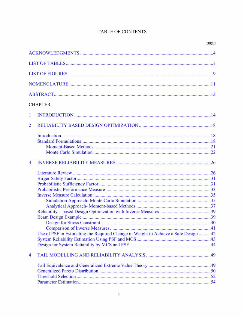
TABLE OF CONTENTS page

ACKNOWLEDGMENTS ...............................................................................................................4

LIST OF TABLES...........................................................................................................................7

LIST OF FIGURES .........................................................................................................................9

NOMENCLATURE ......................................................................................................................11

ABSTRACT...................................................................................................................................13

CHAPTER

1 INTRODUCTION ..................................................................................................................14

2 RELIABILITY BASED DESIGN OPTIMIZATION............................................................18

Introduction.............................................................................................................................18 Standard Formulations............................................................................................................18

Moment-Based Methods .................................................................................................21 Monte Carlo Simulation ..................................................................................................22

3 INVERSE RELIABILITY MEASURES ...............................................................................26

Literature Review ...................................................................................................................26 Birger Safety Factor................................................................................................................31 Probabilistic Sufficiency Factor .............................................................................................31 Probabilistic Performance Measure........................................................................................33 Inverse Measure Calculation ..................................................................................................35

Simulation Approach- Monte Carlo Simulation..............................................................35 Analytical Approach- Moment-based Methods ..............................................................37

Reliability – based Design Optimization with Inverse Measures...........................................39 Beam Design Example ...........................................................................................................39

Design for Stress Constraint ............................................................................................40 Comparison of Inverse Measures ....................................................................................41

Use of PSF in Estimating the Required Change in Weight to Achieve a Safe Design ..........42 System Reliability Estimation Using PSF and MCS..............................................................43 Design for System Reliability by MCS and PSF....................................................................44

4 TAIL MODELLING AND RELIABILITY ANALYSIS ......................................................49

Tail Equivalence and Generalized Extreme Value Theory ....................................................49 Generalized Pareto Distribution .............................................................................................50 Threshold Selection ................................................................................................................52 Parameter Estimation..............................................................................................................54

6

Maximum Likelihood Estimation....................................................................................55 Least Square Regression..................................................................................................56

Accuracy and Convergence Studies for the Quantile Estimation...........................................56 Cantilever Beam Example ......................................................................................................57 Tuned Mass-Damper Example ...............................................................................................59 Alternate Tail Extrapolation Schemes ....................................................................................61

5 MULTIPLE TAIL MODELS.................................................................................................71

Multiple Tail Model................................................................................................................71 Numerical Examples...............................................................................................................72

Standard Statistical Distributions ....................................................................................72 Engineering Examples.....................................................................................................76 Application of multiple tail models for reliability estimation of a cantilever beam........76 Application of multiple tail models for reliability estimation of a composite panel.......77

CONCLUSIONS............................................................................................................................93

APPENDIX

A PSF ESTIMATION FOR A SYSTEM RELIABILITY.........................................................94

B GENERALIZED EXTREME VALUE THEORY.................................................................96

C MAXIMUM LIKELIHOOD ESTIMATION.........................................................................98

D ERROR ANALYSIS FOR GPD ..........................................................................................100

E ACCURACY AND CONVERGENCE STUDIES FOR NORMAL AND LOGNORMAL DISTRIBUTIONS......................................................................................103

F ACCURACY AND CONVERGENCE STUDIES FOR THE CANTILEVER BEAM......108

Stress Failure Mode ..............................................................................................................108 Deflection Failure Mode.......................................................................................................108

G STATISTICAL DISTRIBUTIONS ERROR PLOTS ..........................................................111

REFERENCES ............................................................................................................................121

BIOGRAPHICAL SKETCH .......................................................................................................126

7

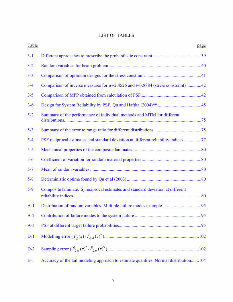
LIST OF TABLES

Table page 3-1 Different approaches to prescribe the probabilistic constraint ..........................................39

3-2 Random variables for beam problem.................................................................................40

3-3 Comparison of optimum designs for the stress constraint .................................................41

3-4 Comparison of inverse measures for w=2.4526 and t=3.8884 (stress constraint) .............42

3-5 Comparison of MPP obtained from calculation of PSF.....................................................42

3-6 Design for System Reliability by PSF, Qu and Haftka (2004)** ......................................45

5-2 Summary of the performance of individual methods and MTM for different distributions........................................................................................................................75

5-3 Summary of the error to range ratio for different distributions .........................................75

5-4 PSF reciprocal estimates and standard deviation at different reliability indices ...............77

5-5 Mechanical properties of the composite laminates............................................................80

5-6 Coefficient of variation for random material properties ....................................................80

5-7 Mean of random variables .................................................................................................80

5-8 Deterministic optima found by Qu et al (2003) .................................................................80

5-9 Composite laminate. rS reciprocal estimates and standard deviation at different reliability indices................................................................................................................80

A-1 Distribution of random variables. Multiple failure modes example ..................................95

A-2 Contribution of failure modes to the system failure ..........................................................95

A-3 PSF at different target failure probabilities........................................................................95

D-1 Modelling error ( ( )gF z - *,

ˆ ( )F zξ σ ). .................................................................................102

D-2 Sampling error ( *,

ˆ ( )F zξ σ - $,

ˆ ( )F zξ σ )................................................................................102

E-1 Accuracy of the tail modeling approach to estimate quantiles. Normal distribution.......104

8

E-2 Accuracy of the tail modeling approach to estimate quantiles. LogNormal distribution .......................................................................................................................105

E-3 Accuracy of the tail modeling approach to estimate quantiles. Higher thresholds. LogNormal distribution ...................................................................................................106

9

LIST OF FIGURES

Figure page 2-1 Reliability analysis and MPP. Subscript refers to iteration number ..................................25

3-1 Schematic probability density of the safety factor S. ........................................................46

3-2 Schematic probability density of the limit state function. .................................................46

3-3 Illustration of the calculation of PPM with Monte Carlo Simulation for the linear performance function .........................................................................................................47

3-4 Inverse reliability analysis and MPP for target failure probability 0.00135 (β = 3)........47

3-5 Cantilever beam subjected to horizontal and vertical loads...............................................47

4-1 Tail modeling of F(u) using the threshold u. The region of y>0 is failure ........................64

4-2 Convergence of PSF at different thresholds. A) MLE B)Regression. Cantilever beam system failure mode. 500 Samples. 100 repetitions...........................................................65

4-3 Tuned vibration absorber ...................................................................................................66

4-4 Normalized amplitude vs r1 and r2.....................................................................................66

4-5 Contour of the normalized amplitude ................................................................................67

4-6 Convergence of PSF at different thresholds. Tuned Mass Damper...................................68

4-7 Tuned Mass Damper. Comparison of tail models using regression and ML method........69

4-8 Transformation of the CDF of PSF reciprocal (Sr). A) CDF of Sr. B) Inverse Standard normal cumulative distribution function applied to the CDF. C ) Logarithmic transformation applied to the reliability index. .............................................70

5-1 Lognormal distribution. Classical tail modeling techniques – MLE and Regression........81

5-2 Lognormal distribution. Linear fit to tail (LT) and Quadratic fit to half of the data (QH) ...................................................................................................................................82

5-3 Lognormal distribution. Quadratic fit to the tail (QT).......................................................83

5-4 Lognormal distribution. Multiple tail models....................................................................84

5-5 Lognormal distribution. Multiple tail models-extrapolation region ..................................85

5-6 Normal distribution. 1000 repetitions. Boxplot comparison of eind and eMTM at different reliability indices.................................................................................................86

10

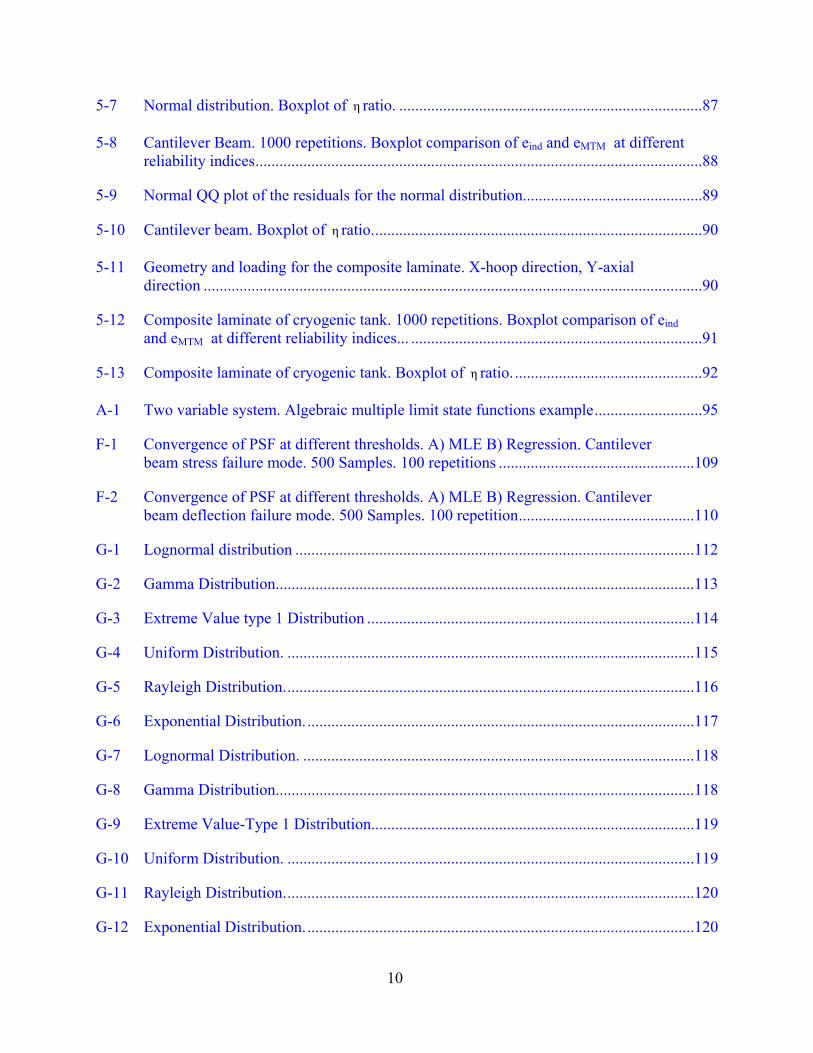
5-7 Normal distribution. Boxplot of η ratio. ............................................................................87

5-8 Cantilever Beam. 1000 repetitions. Boxplot comparison of eind and eMTM at different reliability indices................................................................................................................88

5-9 Normal QQ plot of the residuals for the normal distribution.............................................89

5-10 Cantilever beam. Boxplot of η ratio...................................................................................90

5-11 Geometry and loading for the composite laminate. X-hoop direction, Y-axial direction .............................................................................................................................90

5-12 Composite laminate of cryogenic tank. 1000 repetitions. Boxplot comparison of eind and eMTM at different reliability indices... .........................................................................91

5-13 Composite laminate of cryogenic tank. Boxplot of η ratio. ...............................................92

A-1 Two variable system. Algebraic multiple limit state functions example...........................95

F-1 Convergence of PSF at different thresholds. A) MLE B) Regression. Cantilever beam stress failure mode. 500 Samples. 100 repetitions .................................................109

F-2 Convergence of PSF at different thresholds. A) MLE B) Regression. Cantilever beam deflection failure mode. 500 Samples. 100 repetition............................................110

G-1 Lognormal distribution ....................................................................................................112

G-2 Gamma Distribution.........................................................................................................113

G-3 Extreme Value type 1 Distribution ..................................................................................114

G-4 Uniform Distribution. ......................................................................................................115

G-5 Rayleigh Distribution.......................................................................................................116

G-6 Exponential Distribution..................................................................................................117

G-7 Lognormal Distribution. ..................................................................................................118

G-8 Gamma Distribution.........................................................................................................118

G-9 Extreme Value-Type 1 Distribution.................................................................................119

G-10 Uniform Distribution. ......................................................................................................119

G-11 Rayleigh Distribution.......................................................................................................120

G-12 Exponential Distribution..................................................................................................120

11

NOMENCLATURE

A Cross sectional area

C Capacity

C Scaling factor

CDF Cumulative Density Function

DUU Design Under Uncertainties

FORM First Order Reliability Method

G Limit state function

GPD Generalized pareto distribution

M Number of failure modes

MCS Monte Carlo Simulation

MPP Most Probable Point

MPPIR MPP Inverse Reliability

MPTP Minimum Performance Target Point

MSE Mean square error

PMA Performance Measure Approach

PPM Probabilistic Performance Measure

PSF Probabilistic Sufficiency Factor

R Response

RBDO Reliability based Design Optimization

RIA Reliability Index Approach

RSA Response Surface Approximation

U Variables in standard normal space

u Threshold value

t Thickness

12

w Width

X Load in x direction

Y Load in Y direction

β Reliability Index

Φ Standard Normal Cumulative Density Function

σ Scale parameter

ξ Shape parameter

z Exceedance data

Fu(z) Conditional CDF

( ),F̂ zξ σ Conditional CDF approximated by GPD

targetfP Target probability of failure

13

Abstract of Dissertation Presented to the Graduate School of the University of Florida in Partial Fulfillment of the Requirements for the Degree of Doctor of Philosophy

MULTIPLE TAIL MODELS INCLUDING INVERSE MEASURES FOR STRUCTURAL

DESIGN UNDER UNCERTAINTIES

By

Palaniappan Ramu

December 2007 Chair: Nam Ho Kim Cochair: Raphael T. Haftka Major: Aerospace Engineering

Sampling-based reliability estimation with expensive computer models may be

computationally prohibitive due to a large number of required simulations. One way to alleviate

the computational expense is to extrapolate reliability estimates from observed levels to

unobserved levels. Classical tail modeling techniques provide a class of models to enable this

extrapolation using asymptotic theory by approximating the tail region of the cumulative

distribution function (CDF). This work proposes three alternate tail extrapolation techniques

including inverse measures that can complement classical tail modeling. The proposed approach,

multiple tail models, applies the two classical and three alternate extrapolation techniques

simultaneously to estimate inverse measures at the extrapolation regions and use the median as

the best estimate. It is observed that the range of the five estimates can be used as a good

approximation of the error associated with the median estimate. Accuracy and computational

efficiency are competing factors in selecting sample size. Yet, as our numerical studies reveal,

the accuracy lost to the reduction of computational power is very small in the proposed method.

The method is demonstrated on standard statistical distributions and complex engineering

examples.

14

CHAPTER 1 INTRODUCTION

Uncertainty is an acknowledged phenomenon in the process of structural design. In an

optimization framework design under uncertainties refers to a safe design that not only needs to

be optimal but should also warrant survivability against uncertainties. Traditionally safety factors

were used to account for the uncertainties. However, use of safety factors does not usually lead

to minimum cost designs for a given level of safety because different structural members or

different failure modes require different safety factors. Alternately, probabilistic approaches offer

techniques to characterize the uncertainties using a statistical method and have the potential to

provide safer designs at a given cost. However, the probabilistic approaches require solving an

expensive, complex optimization problem that needs robust formulations and efficient

computational techniques for stable and accelerated convergence. In addition, they also require

statistical information which may be expensive to obtain.

Structural reliability analysis requires the assessment of the performance function which

dictates the behavior of the structure. The performance function is called the limit state function

which is typically expressed as the difference between the capacity (e.g, yield strength, allowable

vibration level) and the response of the system (e.g, stress, actual vibration). Approaches

available for reliability assessment and analysis can be widely classified as analytical and

simulation approaches. Analytical approaches are simple to implement but are mostly limited to

single failure modes, whereas simulation methods like Monte Carlo simulation (MCS) are

computationally intensive but can handle multiple failure modes. Moreover, they can handle any

type of limit state functions unlike analytical approaches which are mostly appropriate for linear

limit state functions. Most real life applications exhibit multiple failure modes and the limit state

function is not available explicitly in closed form. Since there is no information on nonlinearity

15

of the limit state function, MCS is the obvious choice in such situations. In reliability-based

design optimization, a widely used probabilistic optimization approach (Rackwitz, 2000) in

structural engineering, reliability analysis is an iterative process and using crude MCS is

computationally prohibitive. Researchers develop variants of MCS or other approximation

methods like response surface that replaces the reliability analysis and obviate the need to

repeatedly access the expensive computer models

In reliability based design context, high reliability, typical of aerospace applications

translates to small probability in the tails of the statistical distributions. Reliability analysis when

dealing with high reliability (or low failure probability) designs is mostly dependent on how the

tails of the random variables behave. In few cases, the safety levels can vary by an order of

magnitude with slight modifications in the tails of the response variables (Caers and Maes,

1998). Therefore, the tails need to be modeled accurately. Limitations in computational power

prevent us in employing direct simulation methods to model the tails. One way to alleviate the

computational expense is to extrapolate into high reliability levels with limited data at lower

reliability levels. Statistical techniques from extreme value theory referred to as classical tail

modeling techniques here are available to perform this extrapolation. They are based on the

concept of approximating the tail portion of the cumulative distribution function (CDF) with a

generalized pareto distribution (GPD).

In structural engineering, reliability is measured by quantities like probability of failure or

reliability index. Recently, alternate safety measures like the inverse measures in performance

space have cornered enough interest because of their multifaceted advantages (Ramu et al,

2006). The inverse measures in performance space ties the concepts of safety factor and target

failure probability. The inverse measures translate the deficiency in failure probability to

16

deficiency in performance measure and hence provide a more quantitative measure of the

resources needed to satisfy safety requirements. Among the several advantages they exhibit,

inverse measures like probabilistic sufficiency factor (PSF) help in stable and accelerated

convergence in optimization, better response surface approximations compared to surfaces fit to

other reliability measures. Since inverse measure exhibit several advantages, its usefulness in tail

modeling is explored in this work. Here we develop 3 alternate tail extrapolation schemes

including inverse measures that can complement the classical tail modeling techniques. The

alternate extrapolation schemes are based on variable transformations and approximating the

relationship between the inverse measure and transformed variable.

The primary motivation of this work is to develop an efficient reliability estimation

procedure employing tail modeling techniques including inverse measures that can estimate

reliability measures corresponding to high reliability with samples that are only sufficient to

assess reliability measure corresponding to low reliability levels. This is a tradeoff between

accuracy and computational power. Yet, as the studies reveal, the accuracy lost to the reduction

of computational power is very reasonable. The reduction in computational cost is about a

minimum of 3 orders of magnitude for the same level of accuracy.

Goel et al., (2006) developed a method to extend the utility of an ensemble of surrogates.

When faced with multiple surrogates, they explored the possibility of using the best surrogate or

a weighted average surrogate model instead of individual surrogate models. In a similar fashion,

in order to take advantage of both the classical tail modeling techniques and alternate

extrapolation schemes and still come up with the best prediction, we propose to apply all the

techniques simultaneously and use the median of the five estimates as the best estimate. Here, we

call using all the techniques simultaneously as multiple tail models (MTM). In addition to

17

arriving at the estimate, the range of the five techniques can be used to approximate the error

associated with the median estimate. Moreover, the MTM approach can be used to replace the

reliability analysis in reliability based design framework.

.

18

CHAPTER 2 RELIABILITY BASED DESIGN OPTIMIZATION

Introduction

Optimization is the process of minimizing a cost which is a function of design variables

(and other variables) subject to constraints that prescribe the design requirement. Often times, the

variables involved are uncertain and probabilistic approaches are called for to account for the

uncertainty as an alternate to the traditional safety factor approach, to obtain better designs.

Several probabilistic approaches has been proposed in the last decade like Robust Design

Optimization (Phadke, 1989, Gu, 2000), Reliability-based Design Optimization(Frangopal, 1985,

Tu, 1999), Fuzzy optimization (Sakawa 1993, Maglaras et al, 1997), Reliability design using

evidence theory (Soundappan et al., 2004). Reliability-based Design Optimization (RBDO) is

widely used because it allows the designer to prescribe the level of reliability required. This

section presents a review of the standard reliability-based design formulations and reliability

estimation methods.

Standard Formulations

Primarily, reliability-based design consists of minimizing a cost function while satisfying

reliability constraints. The reliability constraints are based on the failure probability

corresponding to each failure mode or a single failure mode describing the system failure. The

estimation of failure probability is usually performed by reliability analysis.

In structural engineering, the system performance criterion is described by the limit state

function which is typically expressed as the difference between the capacity of the system and

the response of the system, which is expressed as:

( ) ( ) ( )c rG G G= −x x x (2-1) where, G is the limit state function and GC, Gr are the capacity and the response respectively. All

the three quantities are functions of a vector x which consists of design (and random) variables

19

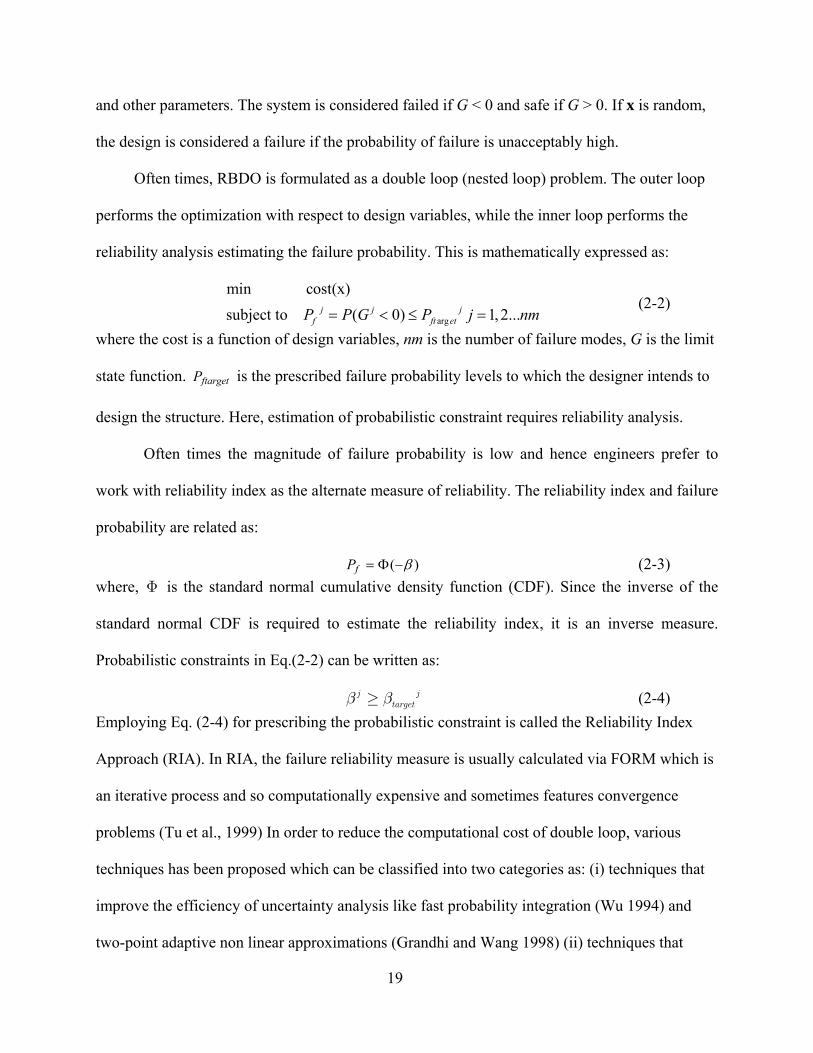
and other parameters. The system is considered failed if G < 0 and safe if G > 0. If x is random,

the design is considered a failure if the probability of failure is unacceptably high.

Often times, RBDO is formulated as a double loop (nested loop) problem. The outer loop

performs the optimization with respect to design variables, while the inner loop performs the

reliability analysis estimating the failure probability. This is mathematically expressed as:

arg

min cost(x)subject to ( 0) 1, 2...j j j

f ft etP P G P j nm= < ≤ = (2-2)

where the cost is a function of design variables, nm is the number of failure modes, G is the limit

state function. ftargetP is the prescribed failure probability levels to which the designer intends to

design the structure. Here, estimation of probabilistic constraint requires reliability analysis.

Often times the magnitude of failure probability is low and hence engineers prefer to

work with reliability index as the alternate measure of reliability. The reliability index and failure

probability are related as:

( )fP β= Φ − (2-3) where, Φ is the standard normal cumulative density function (CDF). Since the inverse of the

standard normal CDF is required to estimate the reliability index, it is an inverse measure.

Probabilistic constraints in Eq.(2-2) can be written as:

≥j jtargetβ β (2-4)

Employing Eq. (2-4) for prescribing the probabilistic constraint is called the Reliability Index

Approach (RIA). In RIA, the failure reliability measure is usually calculated via FORM which is

an iterative process and so computationally expensive and sometimes features convergence

problems (Tu et al., 1999) In order to reduce the computational cost of double loop, various

techniques has been proposed which can be classified into two categories as: (i) techniques that

improve the efficiency of uncertainty analysis like fast probability integration (Wu 1994) and

two-point adaptive non linear approximations (Grandhi and Wang 1998) (ii) techniques that

20

modify the formulation of the probabilistic constraints, for instance, using inverse reliability

measures in the probabilistic constraint. Sometimes, researchers formulate a single loop RBDO

that avoids nested loops. The idea of single loop formulations rests on the basis of formulating

the probabilistic constraint as deterministic constraints by either approximating the Karush-

Kuhn-Tucker conditions at the MPP or approximating the relationship between probabilistic

design and deterministic design safety factors. A detailed survey of both single and double loop

methods in RBDO is presented in the literature survey of Chapter 3.

Kharmanda et al (2002, 2004, and 2007) developed RBDO solution procedures relative to two

views points: reliability and optimization. From an optimization view point, Kharmanda et al

(2002) developed a hybrid method based on simultaneous application of the reliability and the

optimization problem that reduced the computational time. The hybrid method, compared to

classical RBDO, minimizes a new form of the objective function which is expressed as the

product of the original objective function and the reliability index in the hybrid space. Since the

minimization of the objective function is carried out in both the deterministic variables and

random variable space, it is referred to as hybrid design space. The reliability index in the hybrid

space is the distance between the optimum point and the design point in the hybrid space

However, the hybrid RBDO problem was more complex than that of the deterministic design and

may not lead to local optima In order to address both the challenges, Kharmanda et al (2004)

propose an optimum safety factor approach that computes safety factors satisfying a reliability

level without demanding additional computing cost for the reliability evaluation. Kharmanda et

al (2007) developed the hybrid design spaces and optimal safety factor equations for three

distributions namely, the normal, lognormal and uniform. The optimal safety factors are

computed by sensitivity analysis of the limit state function with respect to the random variables.

21

They report that the optimal safety factor approach has several advantages like smaller number

of optimization variables, good convergence stability, lower computing time and satisfaction of

required reliability levels. In order to estimate the reliability measure for reliability analysis, one

need to use analytical or simulation approaches which are described below.

Moment-Based Methods

In standard reliability techniques, an arbitrary random vector x is mapped to an

independent standard normal vector U (variables with normal distribution of zero mean and unit

variance). This transformation is known as Rosenblatt transformation (Rosenblatt, 1952,

Melchers, 1999, pp.118-120). The limit state function in the standard normal space can be

obtained as G(U) =G(T(X)) where T is the transformation. If the limit state function in the

standard normal space is affine, i.e., if (U) UTG α ψ= + , then failure probability can be exactly

calculated as fP ψα

⎛ ⎞= Φ −⎜ ⎟⎜ ⎟

⎝ ⎠ . This is the basis for moment based methods.

Moment-based methods provide for less expensive calculation of the probability of failure

compared to simulation methods, although they are limited to a single failure mode. The First

Order Reliability Method (FORM) is the most widely used moment-based technique. FORM is

based on the idea of the linear approximation of the limit state function and is accurate as long as

the curvature of the limit state function is not too high. In the standard normal space the point on

the first order limit state function at which the distance from the origin is minimum is the MPP.

When the limit state has a significant curvature, second order methods can be used. The

Second Order Reliability Method (SORM) approximates the measure of reliability more

accurately by considering the effect of the curvature of the limit state function (Melchers, 1999,

pp 127-130).

22

Figure 2-1 illustrates the concept of the reliability index and MPP search for a two variable

case in the standard normal space. In reliability analysis, concerns are first focused on the

( ) 0G =U curve. Next, the minimum distance to the origin is sought. The corresponding point is

the MPP because it contributes most to failure. This process can be mathematically expressed as:

To find *Uβ =

Minimize Subject to ( )

TU UG U = 0

(2-5)

Where U* is the MPP. The calculation of the failure probability is based on linearizing the limit

function at the MPP. It is to be noted that reliability index is the distance to the limit state

function from the origin in the standard normal space. That is, it is an inverse measure in the

input space (standard normal).

Monte Carlo Simulation

Variants of Monte Carlo methods were originally practiced under more generic names such

as statistical sampling. The name and the method were made famous by early pioneers such as

Stainslaw Ulam and John von Neumann and is a reference to the famous casino in Monaco. The

methods use of randomness and repetitive nature is similar to the casino’s activities. It is

discussed in Metropolis (1987) that the method earns its name from the fact that Stainslaw Ulam

had an uncle who would borrow money from relative just to go to Monte Carlo.

Monte Carlo integration is essentially numerical quadrature using random numbers. Monte

Carlo integration methods are algorithms for the approximate evaluation of definite integrals,

usually multidimensional ones. The usual algorithms evaluate the integrand at a regular grid.

Monte Carlo methods, however, randomly choose the points at which the integrand is evaluated.

Monte Carlo Methods are based on the analogy between volume and probability. Monte Carlo

calculates the volume of a set by interpreting the volume as probability. Simply put, it means,

23

sampling from all the possible outcomes and considering the fraction of random draws that in a

given set as an estimate of the set’s volume. The law of large numbers ensures that this estimate

converges to the correct value as the number of draws increases. The central limit theorem

provides information about the likely magnitude of the error in the estimate after finite number

of draws.

For example, consider estimating the integral of a function f over a unit interval. The

( )f x dxα1

0

= ∫ (2-6)

integral can be expressed as an expectation [ ]( )E f U , with U uniformly distributed between 0

and 1. The Monte Carlo estimate for the integral can be obtained as:

ˆ ( )n

ii

f Un

α=1

1= ∑ (2-7)

If f is continuous and integrable over [0, 1], then, by the strong law of large numbers, the

estimate in Eq. (2-7) converges to the actual value with probability 1 as n ∞. In fact, if f is

square integrable and we set

( ( ) )f f x dxσ α1

2 2

0

= −∫ (2-8)

then the error α̂ α− in the Monte Carlo estimate is approximately normally distributed with zero

mean and standard deviation of /f nσ , the quality of this approximation improving as n

increases. The parameter fσ in Eq.(2-8) will not be known in a real setting but can be

approximated by the sample standard deviation. Thus, we not only obtain the estimate but also

the error contained in the estimate. The form of the standard error is the main feature of the

MCS. Reducing this error to half require about increasing the number of points by four;

increasing the precision by one decimal point requires 100 times as many points. Yet, the

advantage of MCS lies in the fact that its /( )O n−1 2 convergence rate is not restricted to integrals

24

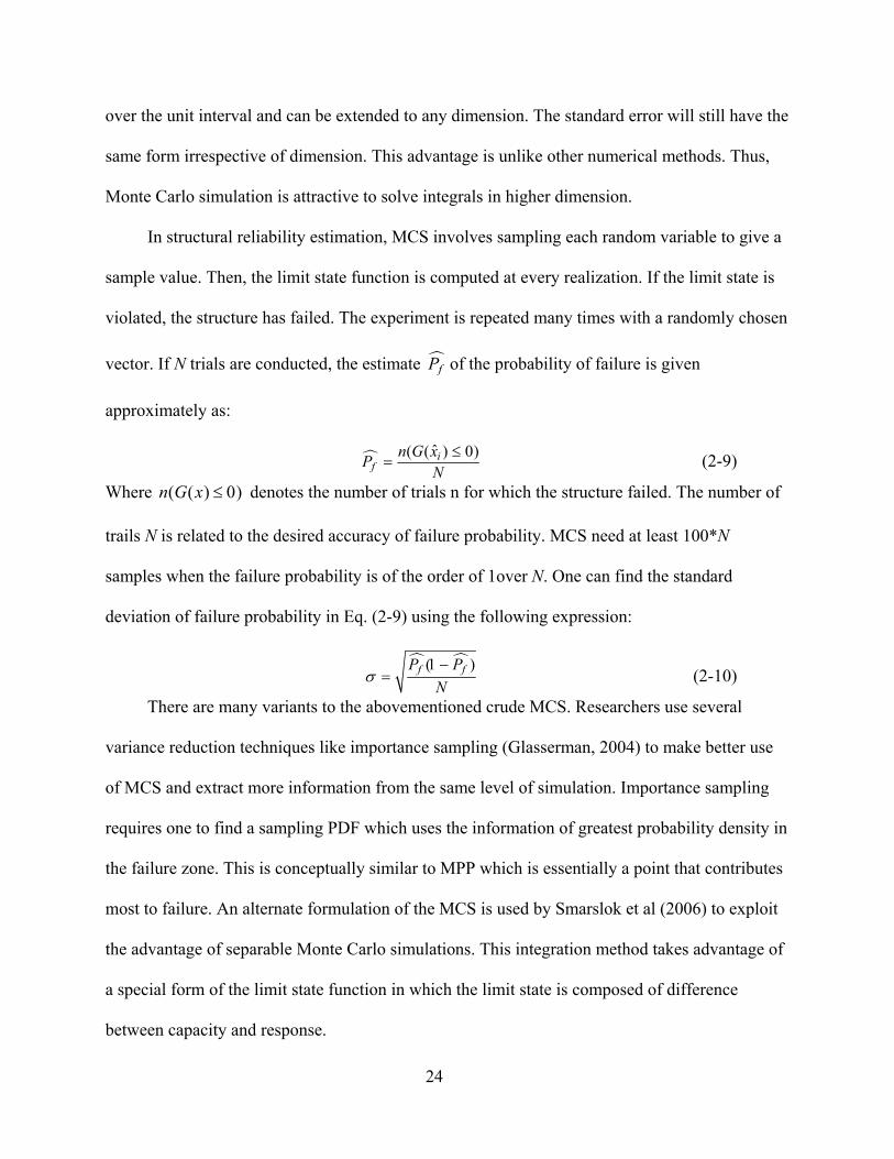
over the unit interval and can be extended to any dimension. The standard error will still have the

same form irrespective of dimension. This advantage is unlike other numerical methods. Thus,

Monte Carlo simulation is attractive to solve integrals in higher dimension.

In structural reliability estimation, MCS involves sampling each random variable to give a

sample value. Then, the limit state function is computed at every realization. If the limit state is

violated, the structure has failed. The experiment is repeated many times with a randomly chosen

vector. If N trials are conducted, the estimate fP of the probability of failure is given

approximately as:

ˆ( ( ) )if

n G xPN

≤ 0= (2-9)

Where ( ( ) )n G x ≤ 0 denotes the number of trials n for which the structure failed. The number of

trails N is related to the desired accuracy of failure probability. MCS need at least 100*N

samples when the failure probability is of the order of 1over N. One can find the standard

deviation of failure probability in Eq. (2-9) using the following expression:

( )f fP P

Nσ

1−= (2-10)

There are many variants to the abovementioned crude MCS. Researchers use several

variance reduction techniques like importance sampling (Glasserman, 2004) to make better use

of MCS and extract more information from the same level of simulation. Importance sampling

requires one to find a sampling PDF which uses the information of greatest probability density in

the failure zone. This is conceptually similar to MPP which is essentially a point that contributes

most to failure. An alternate formulation of the MCS is used by Smarslok et al (2006) to exploit

the advantage of separable Monte Carlo simulations. This integration method takes advantage of

a special form of the limit state function in which the limit state is composed of difference

between capacity and response.

25

Figure 2-1. Reliability analysis and MPP. Subscript refers to iteration number

26

.CHAPTER 3 INVERSE RELIABILITY MEASURES

In probabilistic approaches the difference between the computed probability of failure or

reliability index and their target values does not provide the designer with easy estimates of the

change in the design cost needed to achieve these target values. Alternately, inverse reliability

measures are capable of providing this information. Several inverse reliability measures (e.g.,

probabilistic performance measure and probabilistic sufficiency factor) that are essentially

equivalent have been introduced in recent years. The different names for essentially the same

measure reflect the fact that different researchers focused on different advantages of inverse

measures. This chapter reviews the various inverse measures and describes their advantages

compared to the direct measures of safety such as probability of failure and reliability index.

Methods to compute the inverse measures are also described. Reliability-based design

optimization with inverse measure is demonstrated with a beam design example.

Literature Review

In deterministic approaches, a safety factor is defined as the ratio of the capacity to

resistance of a system, typically calculated at the mean values. However, in probabilistic

approaches, as both capacity and response are random, the safety factor is also a random number.

One safety measure that combines the advantages of the safety factor and probability of failure

was proposed by Birger (1970, as reported by Elishakoff, 2001). Birger relates the safety factor

and the fractile of the safety factor distribution corresponding to a target probability of failure. It

belongs to a class of inverse reliability measures, which carry that name because they require use

of the inverse of the cumulative distribution function. Several researchers developed equivalent

inverse reliability methods (Lee and Kwak 1987; Kiureghian et al. 1994; Li and Foschi 1998; Tu

et al. 1999; Lee et al. 2002; Qu and Haftka 2003; Du et al. 2003) that are closely related to the

27

Birger measure. These measures quantify the level of safety in terms of the change in structural

response needed to meet the target probability of failure.

Lee and Kwak (1987) used the inverse formulation in RBDO and showed that it is preferable for

design when the probability of failure is very low in some region of the design space so that the

safety index approaches infinity. Kiureghian et al. (1994) addressed the inverse reliability

problem of seeking to determine one unknown parameter in the limit state function such that a

prescribed first order reliability index is attained. To solve the inverse reliability problem, they

proposed an iterative algorithm based on the Hasofer-Lind-Rackwitz-Fiessler algorithm. Li and

Foschi (1998) employed the inverse reliability strategy in earthquake and offshore applications to

solve for multiple design parameters. They show that it is an efficient method to estimate design

parameters corresponding to target reliabilities. Kirjner-Neto et al. (1998) reformulated the

standard RBDO formulation similar to Lee and Kwak (1987) except that they use an inequality

constraint. They developed a semi-infinite optimization algorithm to solve the reformulated

problem. This formulation does not require second order derivatives of the limit state functions

and obviates the need for repeated reliability indices computation. However, they found that the

approach can result in conservative design. Royset et al. (2001) extended the reformulation

technique discussed in Kirjner-Neto et al. (1998) for reliability-based design of series structural

systems. The required reliability and optimization calculations are completely decoupled in this

approach. Tu et al. (1999) dubbed the inverse measure approach the Performance Measure

Approach (PMA) and called the inverse measure probability performance measure (PPM). Lee

et al. (2002) adopted the same procedure as Tu et al. (1999) and named it target performance

based approach, calling the inverse measure the target performance. They compared the

reliability index approach and inverse measure based approach and found that the latter was

28

superior in both computational efficiency and numerical stability. Youn et al. (2003) showed that

PMA allows faster and more stable RBDO compared to the traditional Reliability Index

Approach (RIA).

When accurate statistical information is not available for input data, it is not appropriate to

use probabilistic method for stochastic structural analysis and design optimization and

researchers resort to possibility based design optimization (PBDO) methods in such situations.

Mourelatos and Zhou, 2005, discuss a PMA based PBDO. They formulate the inverse possibility

analysis problem for the possibilistic constraint. Unlike FORM based RBDO which is based on

linear approximation, the PBDO is exact. To perform the inverse possibility analysis, Du et al

(2006b) proposes a maximal possibility search (MPS) method with interpolation to address the

challenges of accuracy and computational expense exhibited by traditional methods like the

multilevel cut and alpha level optimization method respectively. They report that the MPS

evaluates possibility constraint efficiently and accurately for nonlinear structural applications.

Often times industry design problems deal with uncertainties with sufficient data and

uncertainties with insufficient data simultaneously. To address such situations Du et al., (2006a)

extend the possibility-based design optimization (PBDO) method. They propose a two step

approach to generate membership function from the available data. Initially, they develop a

temporary PDF using the available data and then generate a membership function from the

temporary PDF. They report that PMA based PBDO combined with MPS method can adequately

address design problems with mixed input variables and demonstrates that it evaluates possibility

constraint efficiently, stably and accurately for nonlinear structural applications.

Qu and Haftka (2003, 2004) called the inverse measure probability sufficiency factor

(PSF) and explored its use for RBDO with multiple failure modes through Monte Carlo

29

Simulation (MCS) and response surface approximation (RSA). They showed that PSF leads to

more accurate RSA compared to RSA fitted to failure probability, provides more effective

RBDO, and that it permits estimation of the necessary change in the design cost needed to meet

the target reliability. Moreover, PSF enables performing RBDO in variable-fidelity fashion and

sequential deterministic optimization fashion to reduce the computational cost (Qu and Haftka,

2004a and 2004b). An initial study of using PSF to convert RBDO to sequential deterministic

optimization was performed to solve problems with reliability constraints on individual failure

modes (Qu and Haftka, 2003). An improved version for system reliability problems with

multiple failure modes was developed for reliability-based global optimization of stiffened

panels (Qu and Haftka, 2004b).

Du et al. (2003, 2004) employed PMA to formulate RBDO, but used percentile levels of

reliability (1 minus failure probability) in the probabilistic constraint and called the inverse

measure as percentile performance. Traditionally, design for robustness involves minimizing the

mean and standard deviation of the performance. Here, Du et al. (2003) proposed to replace the

standard deviation by percentile performance difference, which is the difference between the

percentile performance corresponding to the left tail of a CDF and the right tail of that CDF.

They demonstrated increased computational efficiency and more accurate evaluation of the

variation of the objective performance. In an effort to address reliability-based designs when

both random and interval variables are present, Du and Sudijianto (2003) proposed the use of

percentile performance with worst-case combination of the interval variables for efficient RBDO

solutions.

Du and Chen (2004) developed the sequential optimization and reliability assessment

(SORA) to improve the efficiency of the probabilistic optimization. The method is a serial single

30

loop strategy, which employs percentile performance and the key is to establish equivalent

deterministic constraints from probabilistic constraints. This method is based on evaluating the

constraint at the most probable point of the inverse measure in Section IV below) based on the

reliability information from the previous cycle. This is referred to as “design shift”

(Chiralaksanakul and Mahadevan 2004; Youn et al. 2004). They show that the design quickly

improves in each cycle and is computationally efficient. The sequential optimization and

reliability assessment, however, is not guaranteed to lead to an optimal design. Single-level (or

unilevel) techniques that are equivalent to the standard RBDO formulation are based on

replacing the RIA or PMA inner loop by the corresponding Karush-Kuhn-Tucker conditions.

Here again, Agarwal et al. (2004) showed that the PMA approach is more efficient than the

unilevel RIA approach due to Kuschel and Rackwitz (2000). Since most commercial optimizers

are numerically unreliable when applied to problems accompanied by many equality constraints,

Agarwal et al (2007) use homotopy methods for constraint relaxation and to obtain a relaxed

feasible design. They solve a series of optimization problem as the relaxed optimization problem

is transformed via a homotopy to the original problem. They show that it is easier to solve the

relaxed problem and make a gradual progress towards the solution than solve the original

problem directly.

The several inverse measures discussed above are all based on the common idea of using

the inverse of the cumulative distribution function. The numerous names for the inverse

measures contemplate that they were developed by different researchers for different

applications. Since these inverse measures come under various names, it is easy to fail to notice

the commonality among them.

31

Birger Safety Factor

The safety factor, S is defined as the ratio of the capacity of the system cG (e.g.,

allowable strength) to the response rG with a safe design satisfying r cG G≤ . To account for

uncertainties, the design safety factor is greater than one. For example, a load safety factor of 1.5

is mandated by FAA in aircraft applications. To address the probabilistic interpretation of the

safety factor, Birger (1970) proposed to consider its cumulative distribution function (CDF) SF :

( ) Prob( )cS

r

GF s sG

= ≤ (3-1)

Note that unlike the deterministic safety factor, which is normally calculated for the mean

value of the random variables, c rG G in Eq.(3-1) is a random function. Given a target

probability, ftargetP , Birger suggested a safety factor s* (which we call here the Birger safety

factor) defined in the following equation

Prob( ) Prob( )cS ftarget

r

GF (s*) s* S s* PG

= ≤ = ≤ = (3-2)

That is, the Birger safety factor is found by setting the value of cumulative distribution

function (CDF) of the safety factor equal to the target probability. That is, we seek to find the

value of the safety factor that makes the CDF of the safety factor equal to the target failure

probability. This requires the inverse transformation of the CDF, hence the terminology of

inverse measure.

Probabilistic Sufficiency Factor

Qu and Haftka (2003, 2004) developed a similar measure to the Birger safety factor,

calling it first the probabilistic safety factor and then the probabilistic sufficiency factor (PSF).

They obtained the PSF by Monte Carlo simulation and found that the response surface for PSF

was more accurate than the response surface fitted to failure probability. Later, they found the

32

reference to Birger’s work in Elishakoff’s review (2001) of safety factors and their relations to

probabilities. It is desirable to avoid the term safety factor for this entity because the common

use of the term is mostly deterministic and independent of the target safety level. Therefore,

while noting the identity of the Birger safety factor and the probabilistic sufficiency factor, we

will use the latter term in the following.

Failure happens when the actual safety factor S is less than one. The basic design

condition that the probability of failure should be smaller than the target probability for a safe

design may then be written as:

Prob( 1) (1)f S ftargetP S F P= ≤ = ≤ (3-3) Using inverse transformation, Eq.(3-3) can be expressed as:

11 ( )S ftargetF P s*−≤ = (3-4) The concept of PSF is illustrated in Figure. 3-1. The design requirement ftargetP is known

and the corresponding area under the probability density function of the safety factor is the

shaded region in Figure.3-1.The upper bound of the abscissa s* is the value of the PSF. The

region to the left of the vertical line 1S = represents failure. To satisfy the basic design condition

s* should be greater than or equal to one. In order to achieve this, it is possible to either increase

cG or decrease rG . The PSF s* , represents the factor that has to multiply the response rG or

divide the capacity cG , so that the safety factor be raised to 1.

For example, a PSF of 0.8 means that rG has to be multiplied by 0.8 or cG be divided by

0.8 so that the safety factor ratio increases to one. In other words, this means that rG has to be

decreased by 20 % (1-0.8) or cG has to be increased by 25% ((1/0.8)-1) in order to achieve the

target failure probability. It can be observed that PSF is a safety factor with respect to the target

failure probability and is automatically normalized in the course of its formulation.

33

PSF is useful in estimating the resources needed to achieve the required target probability

of failure. For example, in a stress-dominated linear problem, if the target probability of failure is

10-5 and a current design yields a probability of failure of 10-3, one cannot easily estimate the

change in the weight required to achieve the target failure probability. Instead, if the failure

probability corresponds to a PSF of 0.8, this indicates that maximum stresses must be lowered by

20% to meet the target. This permits the designers to readily estimate the weight required to

reduce stresses to a given level.

Probabilistic Performance Measure

In probabilistic approaches, instead of the safety factor it is customary to use a

performance function or a limit state function to define the failure (or success) of a system. For

example, the limit state function is expressed as in Eq(2-1). In terms of safety factor S, another

form of the limit state function is:

( )( )

( ) 1 1 0c

r

GG S

G= − = − ≥

XX

X (3-5)

Here, ( )G X and ( )G X are the ordinary and normalized limit state functions, respectively. Failure

happens when ( )G X or ( )G X is less than zero, so the probability of failure fP is:

Prob( ( ) 0)fP G= ≤X (3-6) Prob( ( ) 0)fP G= ≤X (3-7) Using Eq. (3-6), Eq. (3-7) can be rewritten as:

Prob( ( ) 0) (0)f G ftargetP G F P= ≤ = ≤X (3-8) Prob( ( ) 0) (0)f ftargetGP G F P= ≤ = ≤X (3-9)

where GF and GF are the CDF of ( )G X and ( )G X , respectively. Inverse transformation allows

us to write Eqs. (3-8) and (3-9) as:

34

10 ( )G ftargetF P g*−≤ = (3-10) 10 ( )ftargetGF P g*−≤ = (3-11)

Here, g* and g* are the ordinary and normalized Probabilistic Performance Measure (PPM, Tu

et al, 1999), respectively. PPM can be defined as the solution to Eqs. (3-8) and (3-9). That is, the

value in (•) (instead of zero) which makes the inequality an equality. Hence PPM is the value of

the limit state function that makes its CDF equals the target failure probability. Figure 3-2

illustrates the concept of PPM. The shaded area corresponds to the target failure probability. The

area to the left of the line 0G = indicates failure. g* is the factor that has to be subtracted from

Eq. (3-6) in order to make the vertical line g* move further to the right of the 0G = line and

hence facilitate a safe design.

For example, a PPM of -0.8 means that the design is not safe enough, and -0.8 has to be

subtracted from ( )G X in order to achieve the target probability of failure. A PPM value of 0.3

means that we have a safety margin of 0.3 to reduce while improving the cost function to meet

the target failure probability.

Considering g* as the solution for Eq.(3-11), it can be rewritten in terms of the safety

factor as:

Prob( ( ) 1 ) ftargetG S g* P= − ≤ =X (3-12)

Comparing Eqs. (15), (23) and (24), we can observe a relationship between s* and g* . PSF

( s* ) is related to the normalized PPM ( g* ) as:

1s* = g* + (3-13) This simple relationship between PPM and PSF shows that they are closely related, and the

difference is only in the way the limit state function is written. If the limit state function is

expressed as the difference between capacity and response as in Eq.(3-6), failure probability

35

formulation allows us to define PPM. Alternatively, if the limit state function is expressed in

terms of the safety factor as in Eq. (3-7), the corresponding failure probability formulation allows

us to define PSF. PSF can be viewed as PPM derived from the normalized form of Eq. (3-6). The

performance-measure approach (PMA) notation may appeal because of its generality, while the

PSF notation has the advantage of being automatically scaled and being expressed in terms that

are familiar to designers who use safety factors.

The PPM can be viewed as the distance from the G = 0 to target failure probability line, in

the performance function space. This is analogical to reliability index being a measure of

distance in the input variable space. The major difference is the measurement of distance in

different spaces, the performance function (or output) space and the input space.

Inverse Measure Calculation

Simulation Approach- Monte Carlo Simulation

Conceptually, the simplest approach to evaluate PSF or PPM is by Monte Carlo simulation

(MCS), which involves the generation of random sample points according to the statistical

distribution of the variables. The sample points that violate the safety criteria in Eq. (3-6) are

considered failed. Figure.3-3 illustrates the concept of MCS. A two-variable problem with a

linear limit state function is considered. The straight lines are the contour lines of the limit state

function and sample points generated by MCS are represented by small circles, with the

numbered circles representing failed samples. The zero value of the limit state function divides

the distribution space into a safe region and a failure region. The dashed lines represent failed

conditions and the continuous lines represent safe conditions.

The failure probability can be estimated using Eq.(2-9) In Figure. 3-3, the number of

sample points that lie in the failure region above the 0G = curve is 12. If the total number of

36

samples is 100,000, the failure probability is estimated at 1.2x10-4. For a fixed number of

samples, the accuracy of MCS deteriorates with the decrease in failure probability.

For example, with only 12 failure points out of the 100,000 samples, the standard deviation

of the probability estimate is 3.5x10-5, more than a quarter of the estimate. When the probability

of failure is significantly smaller than one over the number of sample points, its calculated value

by MCS is likely to be zero.

PPM is estimated by MCS as the thn smallest limit state function among the N sampled

functions, where ftargetn N P= × . For example, considering the example illustrated in Figure. 3-3,

if the target failure probability is 10-4, to satisfy the target probability of failure, no more than 10

samples out of the 100,000 should fail. So, the focus is on the two extra samples that failed.

PPM is equal to the value of the highest limit state function among the n (in this case, n = 10)

lowest limit state functions. The numbered small circles are the sample points that failed. Of

these, the three highest limit states are shown by the dashed lines. The tenth smallest limit state

corresponds to the sample numbered 8 and has a limit state value of -0.4, which is the value of

PPM. Mathematically this is expressed as:

ii = 1( ( ))

Nthg* n min G= X (3-14)

where, thn min is the thn smallest limit state function. So, the calculation of PPM in MCS

requires only sorting the lowest limit state function in the MCS sample. Similarly, PSF can be

computed as the nth smallest factor among the N sampled safety factors and is mathematically

expressed as **:

ii = 1( ( ))

Nths* n min S= X (3-15)

** A more accurate estimate of PPM or PSF will be obtained from the average of the nth and (n+1)th smallest values. So in the case of Figure. 4, PPM is more accurately estimated as 0.35.

37

Finally, probabilities calculated through Monte Carlo Simulation (MCS) using a small

sample size are computed as zero in the region where the probability of failure is lower than one

over the number of samples used in MCS. In that region, no useful gradient information is

available to the optimization routine. On the other hand, PSF value varies in this region and thus

provides guidance to optimization.

MCS generates numerical noise due to limited sample size. Noise in failure probability

may cause RBDO to converge to a spurious minimum. In order to filter out the noise, response

surface approximations are fitted to failure probability to create a so-called design response

surface. It is difficult to construct a highly accurate design response surface because of the huge

variation and uneven accuracy of failure probability. To overcome these difficulties, Qu and

Haftka (2003, 2004) discuss the usage of PSF to improve the accuracy of the design response

surface. They showed that design response surface based on PSF is more accurate compared to

design response surface based on failure probability and this accelerates the convergence of

RBDO. For complex problems, response surface approximations (RSA) can also be used to

approximate the structural response in order to reduce the computational cost. Qu and Haftka

(2004b) employ PSF with MCS based on RSA to design stiffened panels under system reliability

constraint.

Analytical Approach- Moment-based Methods

Inverse reliability measures can be estimated using moment based methods like FORM.

The FORM estimate is good if the limit state is linear but when the limit state has a significant

curvature, second order methods can be used. The Second Order Reliability Method (SORM)

approximates the measure of reliability more accurately by considering the effect of the

curvature of the limit state function (Melchers, 1999, pp 127-130).

38

Figure 3-4. illustrates the concept of inverse reliability analysis and MPP search. The

circles represent the β curves with the target β curve represented by a dashed circle. Here,

among the different values of limit state functions that pass through the targetβ curve, the one

with minimum value is sought. The value of this minimal limit state function is the MPP as

shown by Tu et al. 1999. The point on the target circle with the minimal limit state function is

sought. This point is also an MPP and in order to avoid confusion between the usual MPP and

MPP in inverse reliability analysis, Du et al. (2003) coined the term most probable point of

inverse reliability (MPPIR) and Lee et al. (2002) called it the minimum performance target point

(MPTP). Du et al. (2003) developed the sequential optimization and reliability analysis method

in which they show that evaluating the probabilistic constraint at the design point is equivalent to

evaluating the deterministic constraint at the most probable point of the inverse reliability. This

facilitates in converting the probabilistic constraint to an equivalent deterministic constraint. That

is, the deterministic optimization is performed using a constraint limit which is determined based

on the inverse MPP obtained in the previous iteration. Kiureghian et al. (1994) proposed an

extension of the Hasofer-Lind-Rackwitz-Fiessler algorithm that uses a merit function and search

direction to find the MPTP. In Figure 3-4, the value of the minimal limit state function or the

PPM is -0.2. This process can be expressed as:

Minimize : ( )

Subject to : U Ttarget

G U

U U β= = (3-16)

In reliability analysis the MPP is on the ( ) 0G =U failure surface. In inverse reliability

analysis, the MPP search is on the targetβ curve. One of the main advantages when inverse

measures are used in the FORM perspective is that, the formulation of the optimization problem

is as expressed in Eq. (3-16) where the constraint has a simple form (circle) compared to the cost

function. The cost function has in general a complicated expression due to the nonlinear

39

transformation between physical random variable X to the standard random variable U. It is well

known that it is easy to satisfy a simple constraint compared to a complicated constraint

irrespective of the cost function. On comparing the formulation in Eq.(2-5) with the formulation

in Eq.(3-16), it is evident that it is easier to solve the latter because of the simpler constraint.

Reliability – Based Design Optimization with Inverse Measures

The probabilistic constraint in RBDO can be prescribed by several methods like the

Reliability Index Approach (RIA), the Performance Measure Approach (PMA), the Probability

Sufficiency Factor approach (PSF), see Table3-1.

Table 3-1. Different approaches to prescribe the probabilistic constraint Method RIA PMA PSF Probabilistic constraint targetβ β≥ 0g* ≥ 1s* ≥ Quantity to be computed Reliability index (β ) PPM ( g* ) PSF ( s* )

In RIA, β can be computed as the product of reliability analysis as

discussed in the previous section. The PPM or PSF can be computed through inverse reliability

analysis or as a byproduct of reliability analysis using MCS.

To date, most researchers have used RIA to prescribe the probabilistic constraint.

However, the advantages of the inverse measures, illustrated in the next section, have led to its

growing popularity.

Beam Design Example

The cantilever beam shown in Figure. 3-5, taken from Wu et al. (2001), is a commonly

used demonstration example for RBDO methods. The length L of the beam is 100". The width

and thickness is represented by w and t. It is subjected to end transverse loads X and Y in

orthogonal directions as shown in the Figure 3-51. The objective of the design is to minimize the

1 For this example, the random variables are shown in bold face

40

weight or equivalently the cross sectional area: A=wt subject to two reliability constraints, which

require the safety indices for strength and deflection constraints to be larger than three. The first

two failure modes are expressed as two limit state functions:

Stress limit: sG R R Y Xwt w t

σ 2 2600 600⎛ ⎞= − = − +⎜ ⎟

⎝ ⎠ (3-17)

Tip displacement limit: - -d O OL Y XG D D D

Ewt t w

3 2 2

2 2

⎛ ⎞4 ⎛ ⎞ ⎛ ⎞= = +⎜ ⎟⎜ ⎟ ⎜ ⎟⎝ ⎠ ⎝ ⎠⎝ ⎠

(3-18)

where R is the yield strength, E is the elastic modulus, D0 the displacement limit, and w and t are

the design parameters. R, X, Y and E are uncorrelated random variables and their means and

standard deviations are defined in Table 3-2.

Table 3-2. Random variables for beam problem Random Variables

X (lb)

Y (lb)

R (psi)

E (psi)

Distribution (μ, σ)

Normal (500,100)

Normal (1000,100)lb

Normal (40000,2000)

Normal (29×106,1.45×106)

Design for Stress Constraint

The design with strength reliability constraint is solved first, followed by the design with a

system reliability constraint. The results for the strength constraint are presented in Table 3-3.

For the strength constraint, the limit state is a linear combination of normally distributed random

variables, and FORM gives accurate results for this case. The MCS is performed with 100,000

samples. The standard deviation in the estimated failure probability is calculated by MCS as:

p1f fP ( P )N

σ−

= (3-19)

In this case, the failure probability of 0.0013 calculated from 100,000 samples has a

standard deviation of 1.14×10-4. It is seen from Table 3-3 that the designs obtained from RIA,

PMA and PSF match well. Since the stress in Eq. (3-17)is a linear function of random variables,

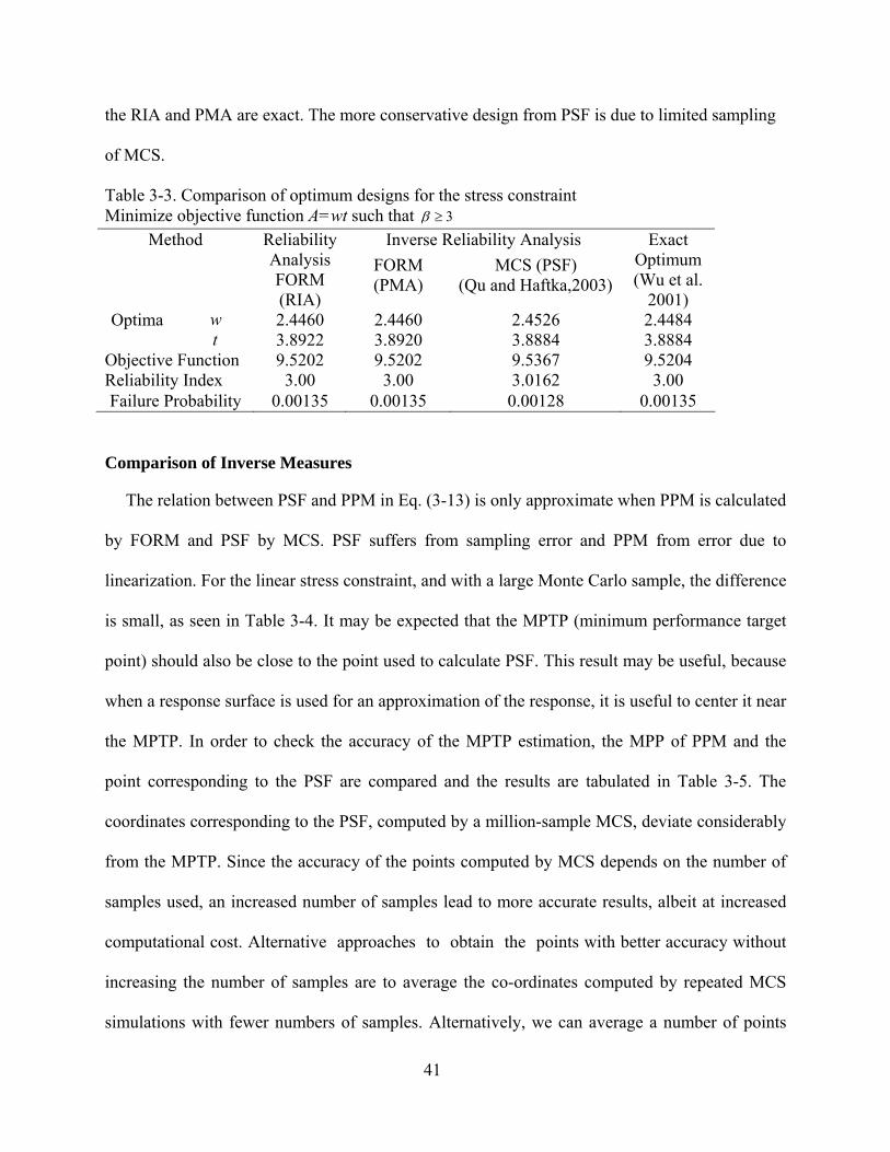
41

the RIA and PMA are exact. The more conservative design from PSF is due to limited sampling

of MCS.

Table 3-3. Comparison of optimum designs for the stress constraint Minimize objective function A=wt such that 3β ≥

Inverse Reliability Analysis Method Reliability Analysis FORM (RIA)

FORM (PMA)

MCS (PSF) (Qu and Haftka,2003)

Exact Optimum (Wu et al.

2001) w 2.4460 2.4460 2.4526 2.4484 Optima t 3.8922 3.8920 3.8884 3.8884

Objective Function 9.5202 9.5202 9.5367 9.5204 Reliability Index 3.00 3.00 3.0162 3.00 Failure Probability 0.00135 0.00135 0.00128 0.00135

Comparison of Inverse Measures

The relation between PSF and PPM in Eq. (3-13) is only approximate when PPM is calculated

by FORM and PSF by MCS. PSF suffers from sampling error and PPM from error due to

linearization. For the linear stress constraint, and with a large Monte Carlo sample, the difference

is small, as seen in Table 3-4. It may be expected that the MPTP (minimum performance target

point) should also be close to the point used to calculate PSF. This result may be useful, because

when a response surface is used for an approximation of the response, it is useful to center it near

the MPTP. In order to check the accuracy of the MPTP estimation, the MPP of PPM and the

point corresponding to the PSF are compared and the results are tabulated in Table 3-5. The

coordinates corresponding to the PSF, computed by a million-sample MCS, deviate considerably

from the MPTP. Since the accuracy of the points computed by MCS depends on the number of

samples used, an increased number of samples lead to more accurate results, albeit at increased

computational cost. Alternative approaches to obtain the points with better accuracy without

increasing the number of samples are to average the co-ordinates computed by repeated MCS

simulations with fewer numbers of samples. Alternatively, we can average a number of points

42

that are nearly as critical as the PSF point. That is, instead of using only the iX corresponding to

the nS in Eq (3-15), we use also the points corresponding to ...,n p n p n pS S S− − +1 + in computing the

PSF, where 2p is the total number of points that is averaged around the PSF. It can be observed

from Table 3-5 that averaging 11 points around the PSF matches well with the MPTP, reducing a

Euclidean distance of about 0.831 for the raw PSF to 0.277 with 11-point average. The values of

X, Y and R presented in Table 3- 5 are in the standard normal space

Table 3-4. Comparison of inverse measures for w=2.4526 and t=3.8884 (stress constraint) Method FORM MCS (1×107samples)Pf 0.001238 0.001241 Inverse Measure PPM: 0.00258 PSF: 1.002619 Table 3-5. Comparison of MPP obtained from calculation of PSF for w=2.4526 and t=3.8884

(stress constraint)

Use of PSF in Estimating the Required Change in Weight to Achieve a Safe Design

The relation between the stresses, displacement and weight for this problem is presented to

demonstrate the utility of PSF in estimating the required resources to achieve a safe design.

Consider a design with the dimensions of A0= w0 t0 with a PSF of 0s * less than one. The

structure can be made safer by scaling both w and t by the same factor c. This will change the

stress and displacement expressed in Eq.(3-17) and Eq. (3-18) by a factor of c3 and c4,

respectively, and the area by a factor of c2. If stress is most critical, it will scale as c3 and the PSF

will vary with the area, A as:

Co-ordinates X Y R MPTP 2.1147 1.3370 -1.6480 PSF 1)106 samples 2.6641 1.2146 -1.0355 2)Average:10 runs of each 105samples 2.1888 1.8867 -1.1097 3)Average:11 points around PSF of 106 Samples 2.0666 1.5734 -1.5128

43

1 5.

*0

0

As* sA

⎛ ⎞= ⎜ ⎟

⎝ ⎠ (3-20)

Equation (3-20) indicates that a one percent increase in area will increase the PSF by 1.5

percent. Since non-uniform scaling of width and thickness may be more efficient than uniform

scaling, this is a conservative estimate. Thus, for example, considering a design with a PSF of

0.97, the safety factor deficiency is 3% and the structure can be made safer with a weight

increase of less than two percent, as shown by Qu and Haftka (2003). For a critical displacement

state, s* will be proportional to 2A and a 3% deficit in PSF can be corrected in under 1.5%

weight increase. While for more complex structures we do not have analytical expressions for

the dependence of the displacements or the stresses on the design variables, designers can

usually estimate the weight needed to reduce stresses or displacements by a given amount.

System Reliability Estimation Using PSF and MCS

System reliability arises when the failure of a system is defined by multiple failure modes.

Here, the discussion is limited to series systems. The estimation of system failure probability

involves estimating the failure due to individual modes and failure due to the interaction between

the modes. This is mathematically expressed for a system with n failure modes as:

1 2

1 2 1 3 1

1 2 3 2 1

( ) ( ) ... ( )

( ) ( ) ... ( ) + ( ) ... ( ) ...Higher order terms

sys n

n n

n n n

P P F P F P F

P F F P F F P F FP F F F P F F F

−

− −

= + + +

− ∩ − ∩ − − ∩

∩ ∩ + + ∩ ∩ − (3-21)

It is easy to employ MCS to estimate system failure, as the methodology is a direct extension of

failure estimation for single modes. In the context of employing analytical methods like FORM,

estimation of failure regions bounded by single modes are easy to estimate but estimating the

probability content of odd shaped domains created because of the intersection of two or more

modes is challenging. Techniques are available to estimate the probability content at the

intersection regions but require evaluating multiple integrals (Melchers, pp: 386-400). Since the

44

number of multiple integrals that has to be evaluated depends on the number of variables, the

task becomes arduous when more variables are involved. Instead, an alternate technique is to

develop upper and lower bounds on the failure probability of the structural system. Considering

the terms in the first and the third rows (positive contributions) in Eq. (3-21) permits us to

estimate the upper bound. When the terms in first and second rows (negative contributions) are

considered, the lower bounds can be estimated. Improved bounds for the system reliability are

available in the literature.

Owing to these challenges, MCS is mostly used when system reliability is to be estimated.

As discussed earlier, MCS is computationally prohibitive when the failure probability to be

estimated is low, because of the number of samples required. PSF can be used to estimate system

reliability. The method is an extension of the PSF estimation for single failure mode. When M

failure modes are considered, the most critical safety factor is calculated for each sample. Then

the sorting of the thn minimum safety factor can proceed as in Eq.(3-15). This process is

explained in the flow chart in Figure 3-6. The estimation of PSF for a system reliability case is

demonstrated with an example in Appendix A

Design for System Reliability by MCS and PSF

Monte Carlo simulation is a good method to use for system reliability analysis with

multiple failure modes. For the cantilever beam discussed in the earlier section, the allowable

deflection was chosen to be 2.25" in order to have competing constraints (Wu et al., 2001). The

results are presented in Table 3-6. It can be observed that the contribution of the stress mode to

failure probability dominates the contribution due to displacement and the interaction between

the modes. The details of the design process are provided in Qu and Haftka (2004). They

demonstrated the advantages of using PSF as an inverse safety measure over probability of

failure or the safety index as a normal safety measure. They showed that the design response

45

surface (DRS) of the PSF was much more accurate than the DRS for the probability of failure.

For a set of test points the error in the probability of failure was 39.11% from the DRS to the

PSF, 96.49% for the DRS to the safety index, and 334.78% for the DRS to the probability of

failure.

Table 3-6. Design for System Reliability by PSF, Qu and Haftka (2004)** Optima Objective

Function Pf Safety

Index Pf1 Pf2 Pf1 ∩ Pf2 PSF

*s w = 2.6041 t = 3.6746

9.5691 0.001289 3.01379 0.001133 0.000208 0.000052 1.0006

**100,000 samples, Pf1, Pf2, Pf1 ∩ Pf2 - Failure probabilities due to stress constraint, displacement constraint, and intersection between the modes, respectively.

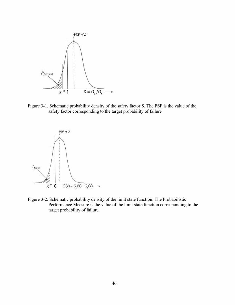
46

Figure 3-1. Schematic probability density of the safety factor S. The PSF is the value of the safety factor corresponding to the target probability of failure

Figure 3-2. Schematic probability density of the limit state function. The Probabilistic

Performance Measure is the value of the limit state function corresponding to the target probability of failure.

47

Figure 3-3. Illustration of the calculation of PPM with Monte Carlo Simulation for the linear performance function

Figure 3-4. Inverse reliability analysis and MPP for target failure probability 0.00135 (β = 3)

Figure 3-5. Cantilever beam subjected to horizontal and vertical loads

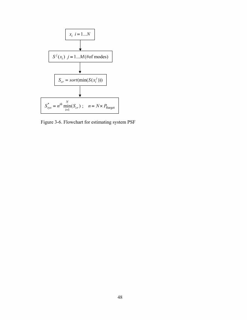
48

Figure 3-6. Flowchart for estimating system PSF

1...ix i N=

( ) 1... (#of modes)jiS x j M=

(min( ( )))jcr iS sort S x=

*ftarget1

min( ) ; N

thsys cri

S n S n N P=

= = ×

49

CHAPTER 4 TAIL MODELLING AND RELIABILITY ANALYSIS

Low failure probability problems (extreme value) require one to have sufficient data in the

tails of the distribution which represent the extremes. But this is seldom possible and instead

researchers use tail modeling techniques based on extreme value theory to predict the probability

of extreme events. The theory comprises a principle for model extrapolation based on the

implementation of mathematical limits as finite level approximations. Since several advantages

are reported by working with inverse measures, it is logical to justify an attempt to perform tail

modeling in the performance space along with inverse measures to estimate quantities at

unobserved levels. This section discusses the tail modeling technique and how to apply it to find

inverse measures.

Tail Equivalence and Generalized Extreme Value Theory

Tail modeling is based on the concept of approximating the tail distribution of the variable

of interest by associating it with the tail of already known distribution and using the parameters

and characteristics therein for further analysis. This criterion is adequately defined by tail

equivalence. That is, two CDFs ( )F x and ( )Q x can be called tail equivalent (Maes and Breitung,

1993) at the right tails when:

1 ( )lim 11 ( )x

F xQ x→ ∞

−=

− (4-1)

This reveals that the error in approximating the small probability of 1- ( )F x by 1- ( )Q x tends to

zero as x →∞ .

The extremal theorem by Fisher and Tippet (1928) states that, if nM is the maximum of a

sequence of ‘n’ independent random variables having a common distribution function and if

there exists sequences of constants { }0na > and{ }nb such that

50

{ }Pr ( ) / ( ) as n n nM b a z H z n− ≤ → →∞ (4-2) for a non-degenerate distribution function H, then H belongs to one of the extreme value

distribution families namely, the Gumbel, Frechet and Weibull families. It is to be noted that

regardless of the distribution for the population, the three types of the extreme value distributions

are the only possible limits for the distribution of the normalized maxima. In this respect, this

theorem is to extreme value theory what central limit theorem is to central statistics. The central

limit theorem states that the approximating distribution of the sample mean is normal regardless

of the parent distribution.

The three families of distributions can be combined into a single family of models having

distribution function of the form

1/

( ) exp 1 zH zξ

μξσ

−⎧ ⎫⎡ − ⎤⎪ ⎪⎛ ⎞= − +⎨ ⎬⎜ ⎟⎢ ⎥⎝ ⎠⎣ ⎦⎪ ⎪⎩ ⎭ (4-3)

such that { }:1 ( ) / 0z zξ μ σ+ − > , where the parameters satisfy μ−∞ < < ∞ , 0σ > and

ξ−∞ < < ∞ . This is the generalized extreme value (GEV) family of distributions. Here, μ is the

location parameter, σ is the scale parameter, ξ is the shape parameter. A more detailed

discussion of the generalized extreme value distributions is presented in Appendix B

Generalized Pareto Distribution

In engineering applications, rather than maxima, the interest is to address the excesses over

threshold. In these situations, the generalized pareto distribution (GPD) arises as the limiting

distribution. The concept of GPD is presented in Figure 4-1. Let y be a model output which is

random and u be a large threshold of y. The observations of y that exceed u are called

exceedance. The conditional distribution ( )uF z of the exceedance given that the data y is greater

than the threshold u, is modeled fairly well by the GPD. Here, z y u= − . Let approximation of

51

( )uF z using GPD be denoted by ,ˆ ( )F zξ ψ . and ξ ψ are the shape and scale parameters

respectively. For a large enough u, the distribution function of ( )y u− , conditional on y > u, is

approximately written as (Coles, 2001):

( )

1

,

1 1 if 0ˆ

1 exp if =0

zF z

z

ξ

ξ σ

ξ ξψ

ξψ

−

+

⎧⎪ − + ≠⎪

= ⎨⎪ ⎛ ⎞

− −⎪ ⎜ ⎟⎝ ⎠⎩

(4-4)

In Eq (4-4), max(0, )A A+= and 0z > .ξ plays a key role in assessing the weight of the

tail. Eq (4-4) can be justified as a limiting distribution as u increases (Coles, 2001, pp:75-76).

Tails can be classified based on ξ as:

0, heavy tail (pareto type tail)0, medium tail (exponential type tail)0, light tail (Beta-type tails)

ξξξ

>=<

There are several parameter estimation methods to estimate the parameters and ξ ψ .It is to be

noted that conditional excess CDF ( )uF z is related to the CDF of interest ( )F y through the

following expression:

( ) ( )( )1 ( )u

F y F uF zF u−

=−

(4-5)

From Eq (4-5), the CDF of y can be expressed as:

( ) (1 ( )) ( ) ( )uF y F u F z F u= − + (4-6) When Eq (4-4) is substituted for ( )uF z in the above expression, Eq (4-6) becomes:

( )1

( ) 1 1 ( ) 1 ( )F y F u y uξξ

ψ

−

+

= − − + − (4-7)

For simplicity of presentation, only the case of 0ξ ≠ is considered here. Once we obtain

estimates of the parameters as and ξ ψ using some parameter estimation method like maximum

52

likelihood estimation method, least square regression that are discussed later in the chapter, it is

possible to estimate the pth quantile by inverting Eq.(4-7) :

1 1 ( )( ) 11 ( )p

F py F p uF u

ξψξ

−

−⎛ ⎞⎛ ⎞−⎜ ⎟= = + −⎜ ⎟−⎜ ⎟⎝ ⎠⎝ ⎠

(4-8)

In order to extend the concept to structural applications, if the output y is replaced by the

limit state in Eq (3-5) then the interest is to model the lower tail rather than the upper tail.

However, modeling the upper tail of y is equivalent to modeling the lower tail of –y. Therefore,

an equivalent way of expressing Eq.(3-5) is:

1( ) 1 ( )rG x S x= − (4-9) where rS is the reciprocal of the safety factor. Failure occurs when G1 > 0. rS at any required

target reliability index can be estimated using Eq(4-8). If targetfP refers to the target failure

probability that we wish to design the structure, PSF can be obtained as:

( )ˆ

target1 target

ˆ1 1ˆ 1 ( )

fr f

PS F P u

F u

ξψξ

−

−⎡ ⎤⎛ ⎞⎢ ⎥= − = + −⎜ ⎟−⎢ ⎥⎝ ⎠⎣ ⎦

(4-10)

Coles (2001) opines that it is easy to object to the procedure of tail modeling on the

grounds that even with the support of asymptotic argument, there is an implicit assumption that

the underlying stochastic mechanism of the process being modeled is sufficiently smooth to

enable extrapolation. However no credible alternative has been proposed to date.

Threshold Selection

The theory of excess over threshold is referred to as peaks over threshold method also.

Performance of this approach is based on the choice of the threshold value u. The basic theory

identified by Pickands (1975) states that the pareto distribution will be a practical family for

statistical estimation of the tails, provided that the threshold is taken sufficiently high. The CDF

is composed of 3 portions, the lower tail, upper tail and the central portion. In theory, the

53

threshold should be selected where the actual upper tail starts. But there is no straightforward

globally accepted method to select threshold.

Selection of threshold is a tradeoff between bias and variance. If the threshold selected is

low, then some data points belong to the central part of the distribution and do not provide a

good approximation to the tails. On the other hand, if the threshold selected is too high, the

number of data available for the tail approximation is much less and this might lead to excessive

scatter in the final estimate. The proper selection of threshold is very important because it has

important repercussions on the estimated value of the shape factor (Caers and Maes, 1998,

McNeil and Saladin, 1997) and hence on the final estimates such as the quantile, extreme values

etc.

There are many exploratory techniques like the mean excess plot which help in selecting

the threshold. But in a simulation study, it is impractical to perform interactive data analysis

required by the exploratory techniques to choose the threshold. The mean excess plot is the

sample mean excess function defined as the sum of the excesses over the threshold divided by

the number of the data points which exceed the threshold plotted with respect to the threshold. A

reasonable choice of the optimal threshold is where this plot becomes linear. For further reading

the reader is referred to Coles (2001).

Boos (1984) suggests that the ratio of Nex (number of tail data) over N (total number

data) should be 0.02 (50<N<500) and the ratio should be 0.1 for 500<N<1000. Hasofer (1996)

suggests using 1.5Nex N= . Caers and Maes (1998) propose to use a finite sample mean square

error (MSE) as a criterion for estimating the threshold. They use the threshold value that

minimizes the MSE. In a similar fashion Beirlant et al (1996) find an optimal threshold by

minimizing an approximate expression for asymptotic mean square error. The other methods

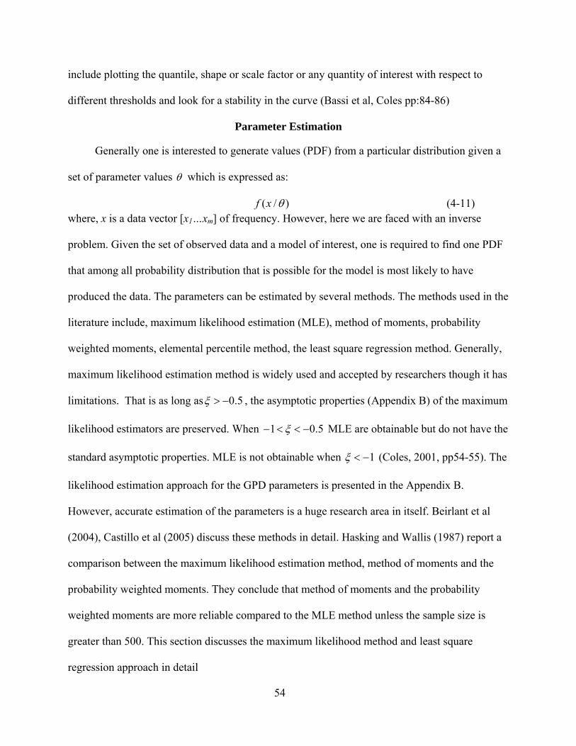
54

include plotting the quantile, shape or scale factor or any quantity of interest with respect to

different thresholds and look for a stability in the curve (Bassi et al, Coles pp:84-86)

Parameter Estimation

Generally one is interested to generate values (PDF) from a particular distribution given a

set of parameter values θ which is expressed as:

( / )f x θ (4-11) where, x is a data vector [x1…xm] of frequency. However, here we are faced with an inverse

problem. Given the set of observed data and a model of interest, one is required to find one PDF

that among all probability distribution that is possible for the model is most likely to have

produced the data. The parameters can be estimated by several methods. The methods used in the

literature include, maximum likelihood estimation (MLE), method of moments, probability

weighted moments, elemental percentile method, the least square regression method. Generally,

maximum likelihood estimation method is widely used and accepted by researchers though it has

limitations. That is as long as 0.5ξ > − , the asymptotic properties (Appendix B) of the maximum

likelihood estimators are preserved. When 1 0.5ξ− < < − MLE are obtainable but do not have the

standard asymptotic properties. MLE is not obtainable when 1ξ < − (Coles, 2001, pp54-55). The

likelihood estimation approach for the GPD parameters is presented in the Appendix B.

However, accurate estimation of the parameters is a huge research area in itself. Beirlant et al

(2004), Castillo et al (2005) discuss these methods in detail. Hasking and Wallis (1987) report a

comparison between the maximum likelihood estimation method, method of moments and the

probability weighted moments. They conclude that method of moments and the probability

weighted moments are more reliable compared to the MLE method unless the sample size is

greater than 500. This section discusses the maximum likelihood method and least square

regression approach in detail

55

Maximum Likelihood Estimation

MLE is a popular statistical method that is used to make inferences about the parameters of

the underlying probability distribution of a given data set. There is nothing visual about the MLE

method but it is very powerful and is precise for large samples. The likelihood of a set of data is

the probability of obtaining that particular set of data, given the chosen probability distribution

model. ML estimation starts with writing the likelihood function which contains the unknown

distribution parameters. The values of these parameters that maximize the likelihood function are

called the maximum likelihood estimators.

In order to estimate the parameters, the likelihood function has to be constructed by

reversing the roles of the data and parameter in Eq (4-11), i.e.,

( / ) ( / )L x f xθ θ= (4-12) Thus L represent the likelihood of the parameter θ given the observed data x and is a function

ofθ . For a model with k parameters, the likelihood function takes the shape of k-dim geometrical

surface sitting above a k-dim hyperplane spanned by the parameter vector (Myung, 2003).

Both f and L are PDFs but the major difference lies in the fact that they are defined in two

different axes and are not directly comparable to each other. PDF f is a function of data given a

particular set of parameter values defined on the data scale. The likelihood function L is the

function of parameter given a particular set of observed data defined on the parameter scale.

ML approach is totally analytical in concept. MLE's generally have very desirable large

sample properties (Appendix C) However, MLE cannot be adopted in all situations. There are

some limitations when small numbers of failures (less than 5, and sometimes less than 10 is

small), MLE's can be heavily biased and the large sample asymptotic properties do not apply

56

Least Square Regression

The method of least squares assumes that the best-fit curve of a given type is the curve that

has the minimal sum of the deviations squared (least square error) from a given set of data. The

parameters are obtained by solving the following minimization problem

( )2

,,ˆ ( )

u

N

ii N

Min F z Pξ ψξ ψ=

−∑ (4-13)

The GPD CDF can be obtained by using Eq. (4-4). The empirical CDF are plotting positions

which are computed as:

,i=1...1i

iP NN

=+

(4-14)

where N is the total number of samples, Nu is the index corresponding to the threshold u and P is

the plotting position. Since it is a minimum finding, it can be seen as an optimization technique

similar to maximum likelihood estimate method where we try to maximize the likelihood

function. Least square regression requires no or minimal distributional assumptions. Unlike

MLE, there is no basis for testing hypotheses or constructing confidence intervals.

Accuracy and Convergence Studies for the Quantile Estimation

In order to understand the capability of GPD to model the tails of the distribution, an error

analysis in terms of modeling and sampling error was performed on the probability content

estimation using tail modeling approach. A detailed discussion of this is presented in Appendix

D. Based on the results, it can be concluded that the sampling error is high compared to the

modeling error. If the sampling error is accounted for, tail modeling has a fairly good capacity to

estimate extreme probabilities with good accuracy. . In structural reliability studies, one is

required to model the tails of the response which might follow some standard statistical

distributions. Normal and Lognormal distributions are widely used to model physical quantities

in structural reliability studies. Therefore, an investigation was done to study the accuracy and

57

convergence capabilities of tail modeling approach to model the tails of normal and lognormal

distribution which is discussed in detail in Appendix E. Then, the approach is demonstrated on a

cantilever beam example and a tuned mass damper example to estimate the failure probability.

The simulation studies (Appendix E) help us to conclude that based on the target quantile

value we wish to estimate, the threshold and number of exceedance data need to be chosen. In

the context of structural analysis, the interest is to address the response function. The failure

probability is based on the response. If we wish to design a system with a low failure probability

of the order of 1e-4 or higher, then we are required to estimate quantiles of 0.9999 or higher. So,

if the response follows a distribution close to normal, and we wish to estimate a quantile of

0.9999, a quantile of 0.95 and 100 exceedance data would enable us to estimate the quantile

under 3% error. On the other hand, if the response follows more of a lognormal distribution

(heavy tailed), then one is required to choose a higher threshold of the order of 0.99 or 0.995

with 100 or more exceedance data to be guaranteed to have a bias error of less than one percent

and a RMSE error of less than 5 percent. However, it is not possible to come up with a table that

explains the minimum exceedance data required for a level of quantile and required accuracy

level because, in practical situations the distribution of the response is not known. Moreover, the

challenge is to develop methodologies that can estimate the inverse measure corresponding to

high reliability, with limited samples.

Cantilever Beam Example

The beam example that was considered in Chapter 3 is treated here also. Though

simulating the beam example is not very expensive, we pretend that we have limited computer

resources and are restricted to use a maximum of 500 simulations. We are interested in

estimating the PSF for low failure probabilities with only 500 response data. Three different

cases are discussed. Case 1 discusses the estimation of PSF for the strength failure mode using

58

the tail modeling approach at different threshold values. Similarly the PSF estimation for the

deflection failure mode is investigated in Case 2 and the system failure case where both the

failure modes are considered simultaneously is discussed in Case 3. Case 1 and Case 2 are

presented in Appendix F. For all the cases, the convergence of PSF with respect to different

thresholds and accuracy of PSF at different number of samples are investigated. Two methods,

namely the maximum likelihood method and the least square regression methods are used to

estimate the parameters. The results from these methods are compared.

In the system failure mode, both the failure modes are considered simultaneously. The safety

factor for each failure mode is evaluated. For each realization, the critical of the two safety factor

is considered the system safety factor. Once, the system safety factor is obtained for 100

simulations, the tail modeling approach is carried out and the corresponding system PSF is

estimated. Here the design variables are w=2.6041; t=3.6746 and the allowable deflection

D0=2.145. This combination of the variables allows equal contribution of the modes to the total

failure. The contribution of the modes are: 1 0.00099fP = ; 2 0.00117fP = ; 1 2 0.00016f fP P∩ = .

The convergence plots of PSF for the system failure case is presented in Figure 4-2. Figure 4-2

shows that the PSF estimated through parameters estimated by the regression method is unstable

in contrast to the PSF estimated through parameters from the ML method. This behavior was

observed in the other two cases too. The PSF estimate at a threshold of 0.9 is 0.99 with a

standard deviation of 0.003. The corresponding failure probability estimate is 0.0017 with a

standard deviation of 0.0002 which is about 10% of the estimate. The number of samples used in

the above studies is 500. The PSF is expected to converge to the actual value when the number

of samples is increased.

59

Tuned Mass-Damper Example

The tail modeling approach to estimate the failure probability is demonstrated here with

the help of a tuned mass-damper example. The tuned mass-damper problem in Figure 4-3 is

taken from Chen et al (1999). The problem involves the failure probability estimation of a

damped single degree of freedom system with dynamic vibration absorber. Figure 4-3 illustrates

the tuned damper system consisting of the single degree of freedom system and a dynamic

vibration absorber to reduce the vibrations. The original system is externally excited by a

harmonic force. The absorber serves to reduce the vibration. The amplitude of vibration depends

on

mRM

= , the mass ratio of the absorber to the original system

ζ, the damping ratio of the original system

11

nr ωω

= , ratio of the natural frequency of the original system to the excitation frequency

22

nr ωω

= , ratio of the natural frequency of the absorber to the excitation frequency

The amplitude of the original system y is normalized by the amplitude of its quasi static

response and is a function of four variables expressed as:

2

2

2 22 2 22

2 2 21 1 2 1 2 1 1 2

11

1 1 1 1 1 11 4

ry

Rr r r r r r r r

ζ

⎛ ⎞− ⎜ ⎟⎝ ⎠

=⎡ ⎤ ⎡ ⎤⎛ ⎞ ⎛ ⎞ ⎛ ⎞ ⎛ ⎞− − − + + −⎢ ⎥ ⎢ ⎥⎜ ⎟ ⎜ ⎟ ⎜ ⎟ ⎜ ⎟

⎢ ⎥⎝ ⎠ ⎝ ⎠ ⎝ ⎠ ⎝ ⎠⎣ ⎦⎣ ⎦

(4-15)

This example treats 1 2 and r r as random variables. They follow a normal distribution

N(1,0.025) and 0.01, =0.01R ζ= . The normalized amplitude of the original system is plotted in

60

Figure 4-4. There are two peaks where the normalized amplitude reached undesirable vibration

levels. The corresponding contour plot is presented in Figure 4-5. The failure region is denoted

by the red band. This failure region is an island. That is, the failure region has safe regions on

either side of it. This introduces additional challenges of not being able to use analytical

approaches like FORM because the failure region is not a half plane. The objective of the

problem is to reduce the risk of the normalized amplitude being larger than a certain value. The

limit state for this case is expressed as:

1 2 1 2 0( , ) ( , )g r r y r r y= − (4-16) where 0y can be considered as the allowable level of vibration. When the limit state in Eq.

(4-16) is greater than 0, failure is said to occur. Increasing or decreasing 0y will help in

decreasing or increasing the failure probability respectively. 0y =27 is considered for the

discussion. The corresponding failure probability with 1e7 sample MCS is estimated to be

0.01031. The tail modeling approach with 500 samples and 100 repetitions are used to study the

convergence and accuracy estimates of PSF. The plot for PSF at various thresholds is presented

in Figure 4-6. From the plots, it seems that regression behaves better compared to the ML

method. There is a discrepancy in the plot corresponding to the ML method. The PSF estimated

at 0.96 threshold is more accurate than the PSF estimate at a threshold of 0.98. In order to

understand the behavior of the tail of the tuned mass damper, a log plot of the CDF with 1e5

samples is examined. The plot is presented in Figure 4-7. It is evident from the plot that there are

two curvatures in the tail which are difficult to model. The GPD has to capture this shape with

less exceedance data. This is the reason for the discrepancy in the ML plot, the shape of the tail

at the area of interest (Sr=1) modeled by ML with a threshold of 0.96 was better than the tail

model with a threshold of 0.98.

61

In order to further explore the tail models from each method, the tail model from each

method is superimposed on each other and the comparative plots are presented in Figure 4-7. It is

clearly observed that the tail modeled based on ML approach denoted by the dashed line

attempts to capture the second curvature and in the process introduces error in the PSF value

corresponding to a failure probability level of 0.01. On the other hand, the model obtained based

on regression parameters represented by the solid line, approximates the tail in a linear fashion

and is accurate compared to the tail based on ML method for a failure probability of 0.01.

However, the ML method is expected to perform better when the failure probability to be

estimated is low. When the failure probability is low, it becomes necessary to model the second

curvature adequately to estimate the PSF with reasonable accuracy. The ML method can perform

better than the regression approach in modeling the second curvature. Such types of CDF with

double curvature might not be encountered in structural applications often and solving this

problem with less number of samples is very challenging. With more insight on the problem, it is

possible to select the suitable parameter estimation method depending on the requirements. Here,

if one needs to estimate PSF corresponding to failure probabilities lesser than 1e-3, then the

second curvature has to be modeled well and hence ML method is a good choice. Else, for higher

failure probabilities, regression can perform better.

Alternate Tail Extrapolation Schemes

In this section, simple tail extrapolation techniques are developed to estimate the PSF for

low target failure probability using MCS that is sufficient only to estimate the PSF for

substantially higher failure probability (lower target reliability index). Failure probability can be

transformed to reliability index by using Eq. (2-3). The same transformation is applied here to

the CDF of the reciprocal of inverse measure. Since we are modeling the upper tail, reciprocal of

the inverse measure is of interest here. The tail portion of the resulting transformed CDF

62

(relationship between inverse measure and reliability index) is approximated by a linear

polynomial in order to take advantage of fact that normally distributed inverse measure is

linearly related to the reliability index. Since this approximation will not suffice if the inverse

measure follows distributions other than normal, a logarithmic transformation is then applied to

the reliability index which tends to linearize the tail of the transformed CDF. This tail is

approximated using a quadratic polynomial. Since both these techniques use only data from the

tail, another technique that approximates the relationship between inverse measure and reliability

index from the mean to the maximum data using a quadratic polynomial is developed. The three

extrapolation techniques discussed are described with the help of a figure. A data set of size 500

with a mean of 10 and variance 9 following a lognormal distribution is used to illustrate the three

techniques.

Figure 4-8, A) shows the general relationship between PSF reciprocal and 1-Pf. Applying

the transformation modifies the CDF as in B). If the PSF reciprocal follows a normal

distribution, this curve will be linear. Therefore, the first technique approximates the tail of the

curve in B) by a linear polynomial. In order to take advantage of the remaining data, half of the

curve in B) is approximated by a quadratic polynomial. It is sufficient to consider only half of the

data because of the symmetry in reliability index. The third technique applies a logarithmic

transformation to the reliability index and approximates the tail of the curve shown in C) by a

quadratic polynomial. In all the above three techniques, once the coefficients of the polynomial

are obtained, the PSF reciprocal corresponding to any higher reliability index can be found. It is

to be noted that with 500 samples, it is possible to estimate only PSF reciprocal at reliability

levels less than 3. Classical tail models discussed in the previous chapter and the alternate

63

extrapolation techniques discussed in this chapter allow predicting PSF reciprocal at much higher

reliability indices without additional reliability analysis.

The alternative extrapolation techniques and classical tail modeling techniques are

conceptually the same. The major difference in perceiving the two classes is that the classical tail

modeling techniques model the CDF of PSF reciprocal, whereas the extrapolation schemes

approximates the trend of PSF reciprocal in terms of reliability index.

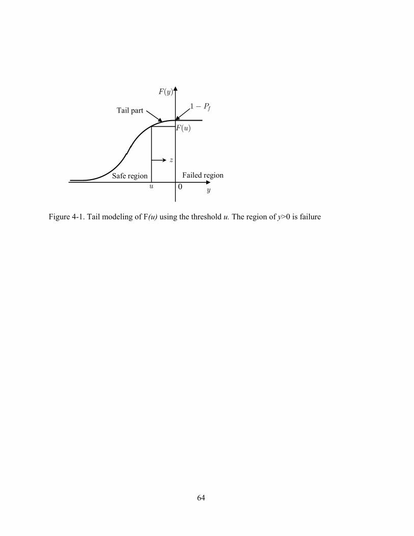
64

0

Tail part

( )F y

( )F u

u y

z

Failed regionSafe region

1 fP−

Figure 4-1. Tail modeling of F(u) using the threshold u. The region of y>0 is failure

65

0.8 0.82 0.84 0.86 0.88 0.9 0.92 0.94 0.96 0.980.95

0.96

0.97

0.98

0.99

1

1.01

1.02

1.03

1.04

1.05

Fu

1/P

SF

LCIUCIMeanMedian

102030405060708090100Nex

A

0.8 0.82 0.84 0.86 0.88 0.9 0.92 0.94 0.96 0.980.9

0.935

0.97

1.005

1.04

1.075

1.11

1.145

1.18

1.215

1.25

Fu

1/P

SF

LCIUCIMeanMedian

102030405060708090100Nex

B Figure 4-2 Convergence of PSF at different thresholds. A) MLE B)Regression. Cantilever beam

system failure mode. 500 Samples. 100 repetitions

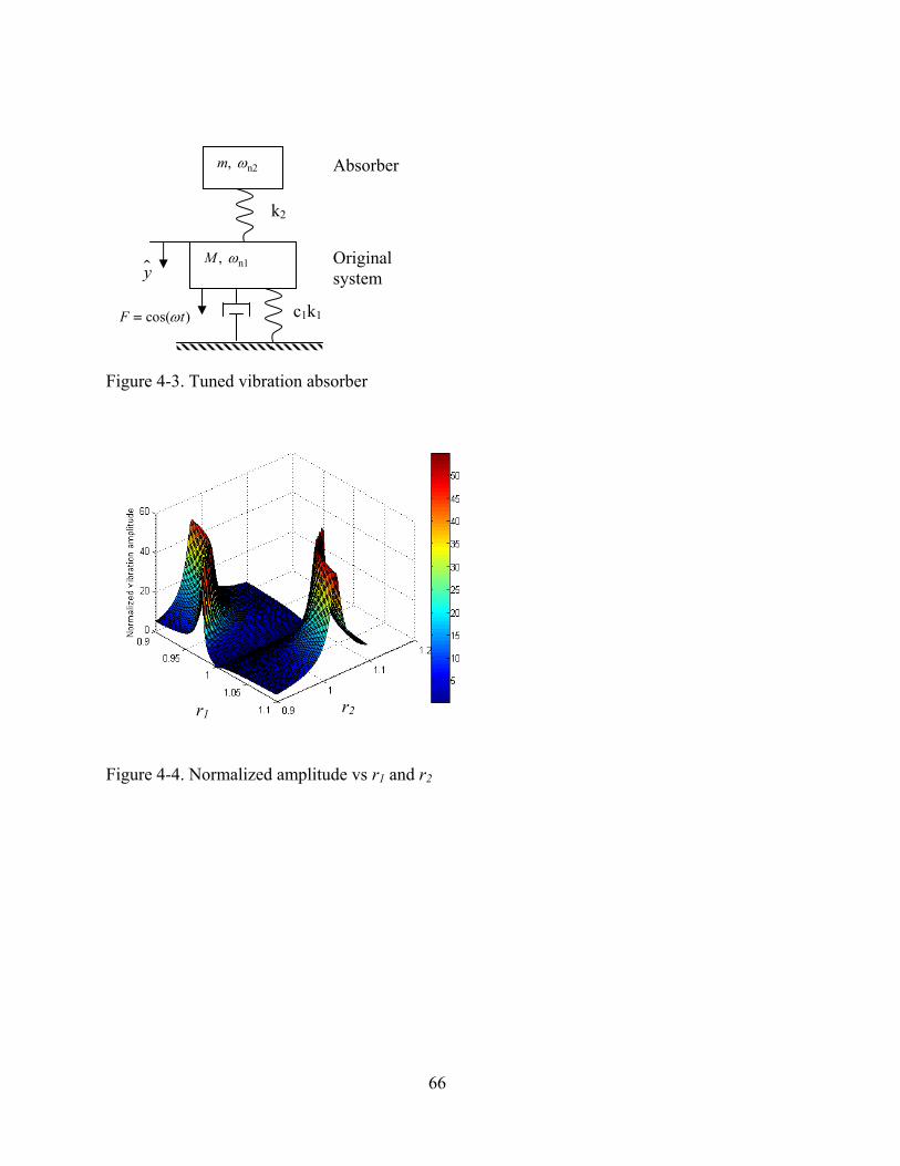
66

Figure 4-3. Tuned vibration absorber

Figure 4-4. Normalized amplitude vs r1 and r2

r1 r2

n2, m ω

n1, M ω

Absorber

Original system

c1k1

y

cos( )F tω=

k2

67

Figure 4-5. Contour of the normalized amplitude

68

0.8 0.82 0.84 0.86 0.88 0.9 0.92 0.94 0.96 0.98 10.6

0.7

0.8

0.9

1

1.1

1.2

1.3

1.4

1.5

1.6

Fu

1/PS

F

Actual PSFLCIUCIMeanMedian

0102030405060708090100Nex

A

0.8 0.82 0.84 0.86 0.88 0.9 0.92 0.94 0.96 0.98 10.6

0.74

0.88

1.02

1.16

1.3

1.44

1.58

1.72

1.86

2

Fu

1/P

SF

Actual PSFLCIUCIMeanMedian

0102030405060708090100Nex

B Figure 4-6. Convergence of PSF at different thresholds. Tuned Mass Damper. A) MLE.

B)Regression. 500 samples. 100 repetitions. LCI – Lower Confidence Interval. UCI- Upper Confidence Interval

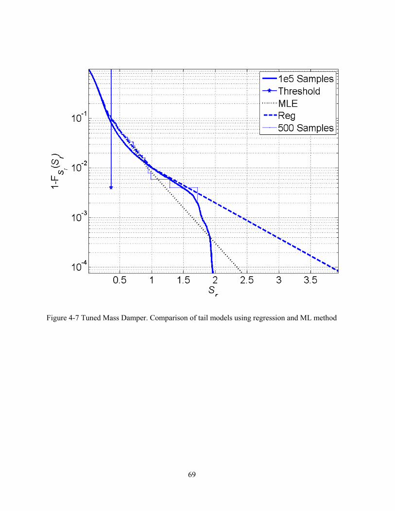
69

Figure 4-7 Tuned Mass Damper. Comparison of tail models using regression and ML method

70

0 0.2 0.4 0.6 0.8 110

−3

10−2

10−1

100

Pf

Sr A

0 0.2 0.4 0.6 0.8 1−3

−2

−1

0

1

2

3

β=φ−1

(1−P

f )

Sr B

0.4 0.5 0.6 0.7 0.8 0.9 1−6

−5

−4

−3

−2

−1

0

1

2

log

(β)

Sr C

Figure 4-8. Transformation of the CDF of PSF reciprocal (Sr). A) CDF of Sr. B) Inverse Standard

normal cumulative distribution function applied to the CDF. C ) Logarithmic transformation applied to the reliability index.

71

CHAPTER 5 MULTIPLE TAIL MODELS

Multiple Tail Model A total of five methods to model the tails of data were discussed in the previous two

sections. However, in practical applications where there is no information on the form of the

output distribution, there is no way to explore which technique performs better. A single

technique that performs well for a particular example might not perform the best for another

example. In fact, a single method that performs the best at a particular reliability index might not

perform the best at a different reliability index for the same example, as will be shown in the

numerical examples. In addition, there are no known straight forward ways to quantify the error

in the estimates.

In order to take advantage of all the techniques and still come up with the best prediction,

we propose to apply the five techniques simultaneously and use the median of the five estimates.

It is observed that the median is a robust estimate than the mean. This method is demonstrated

first on seven different statistical distributions followed by two engineering examples. In all

examples, it is observed that the median of the five estimates is at least the second best compared

to estimates from individual techniques. Moreover, the range of the five estimates closely

approximates the error in the median. Thus using multiple tail models not only ensures to choose

a good estimate and buys insurance against bad predictions but also provides an error of the

estimate. Figures 5.1 to 5.5 show the various tail modeling techniques for a lognormal

distribution with a data mean of 10 and standard deviation of 3. In each case, the 1e5 sample

curve and 500 sample curve are superimposed to highlight the extrapolation. The Sr is computed

as discussed in the implementation in next section. Figure 5.4 shows the multiple tail model

approach (MTM). In order to understand to clearly see the range of the five methods, the region

beyond the threshold is zoomed and presented in Figure 5.5. The range of the five methods at

72

three different reliability indices is marked by double headed arrows. Mean of these ranges

computed over the entire extrapolation zone are capable of representing the error associated with

the median estimate from MTM.A representative actual error is presented in the plot. The QH is

the median and overlaps with the MTM curve.

Numerical Examples

Standard Statistical Distributions

The standard statistical distributions that are discussed in this section are presented in

Table 5-1. A data set with mean 10 and standard deviation 3 is considered. In order to compare

the performance of the proposed method on different distributions, a common target failure

probability is used to find the capacity which is in turn is used to normalize the parameters.

Implementation of this exercise is as follows:

target target0.00135 ( =3), =10, 0.3, =fP x COV COV xβ σ= = ×

1. Use x and COV to estimate parameters ( 0a and 0b ) for each distribution from Table 5-1 . These parameters can be used to generate random numbers.

2. Find capacity C as ( )target1th

fP− quantile. Inverse cumulative distribution functions (icdf) can be used for this. In the case of single parameter distributions, add shift factor to the C.

3. Find normalized mean using xxC

= . We are interested in the safety factor reciprocal , rS

following different statistical distributions. The normalized mean is the mean of the rS . 4. Use x̂ and COV to find new parameters ( a and b ) for all the distributions. 5. Generate N = 500 Latin hypercube samples in [0,1] 6. Find rS at each sample using (a, b) and inverse icdf 7. Use Eq (4-14) to estimate plotting positions 8. Plotting rS and P provides the empirical CDF of rS . It is to be noted that the ordinate is

(1-Pf). That is, we are interested in the upper tail. As Pf decreases, 1- Pf increases, reliability index increases, S decreases and rS increase.

9. A threshold of 0.9 is considered for classical tail modeling techniques and the parameters of GPD that approximates the conditional CDF beyond the threshold are estimated using Maximum Likelihood and least square regression approaches.

10. The transformations discussed in the previous section can be applied to the CDF of rS and rS at higher reliability indices can be estimated directly from the approximated

relationships.

73

11. There are totally five estimates (steps 9 and 10) of rS denoted by indrS in the extrapolated

regions. Record the median and range of indrS .as 5m and 5Ra respectively. 12. Exact values of rS can be obtained using icdf functions.

13. Compute error in the estimate of individual methods eind as abs ( rS - indrS ). 14. Compute error in multiple tail model (MTM) estimate eMTM as abs( rS - 5m) 15. Compute the ratio of mean of eMTM to mean of 5Ra over the entire extrapolation zone and

denote it as η 16. Repeat steps 5 to 15, 1000 times for each distribution. 17. Record the median, mean of eind and eMTM over 1000 repetition as 1000

indm , 1000indμ and

1000MTMm , 1000

MTMμ 18. Record the median and mean of the ratio in step 15 over 1000 repetition as 1000

ηm

For each distribution, boxplots of eind and eMTM are presented. 1000indm and 1000

MTMm compared

at three reliability indices between 3 and 4.2. The results for the normal distribution are

presented in Figure 5-6. The objective of this plot is to see how well the 5m estimate compares to

the indrS . For 1000 repetitions, only the median and the mean can be compared because the range

is volatile. It was observed that the median was a robust estimate compared to the mean. It is

evident that the median is less sensitive to the outliers compared to the mean. At β =3, the

regression (Rg) performs the best followed by the linear tail (LT). The MTM performs as good

as the second best. At β =3.6, the LT performs the best followed by the regression (Rg) and

MTM performs as well as LT. At β =4.2, the LT performs the best followed by the quadratic tail

(QT) and MTM’s performance is as good as LT. It is to be noted that the individual techniques

that provided the best estimate differed at different reliability indices. However, the MTM

estimate was consistent and it performed at least as good as the second best estimate from the

individual techniques. This approach serves as an insurance against bad predictions, if we were

to use a single technique.

74

Box plots of η ratio are presented to see how well the range of the methods compares to

the mean of the eMTM over the entire extrapolation region. The results for the normal distribution

are presented in Figure 5-7. It is clearly observed that the ratio of the mean of the error to the

mean of the range in the entire extrapolation region is around 1. If the ratio is 1, then the range

captures the error in the median perfectly. Here, the range provides an estimate of eMTM that

might slight over or under estimate the actual error. The boxplots for the remaining distributions

are presented in the Appendix G. Table 5-2 provides a summary of the performance of the

individual methods and the MTM for all the distributions. Table 5-2 shows that not a particular

technique was the best for all the distributions and the technique that provided the best estimate

for a particular distribution varied as the reliability indices changed. However, the MTM

estimate was mostly close to the 2nd best available estimate. The summary of η ratio is presented

in Table5-3. It is observed that other than uniform distribution, the ratio varies between 0.15 to

Table 5-1. 7 standard statistical distributions and their parameters

Distribution Parameters a b Normal x σ LogNormal ( ) ( )2ln 0.5x b− 2

ln 1xσ⎡ ⎤⎛ ⎞+⎢ ⎥⎜ ⎟⎝ ⎠⎢ ⎥⎣ ⎦

Gamma 2xσ⎛ ⎞⎜ ⎟⎝ ⎠

aσ

Extreme Type 1

0.577xb

− 6

πσ

Uniform 12

2x σ− 12

2x σ+

Single parameter distributions Exponential x σ− x Rayleigh

( )2

x bπ−

22

σπ

−

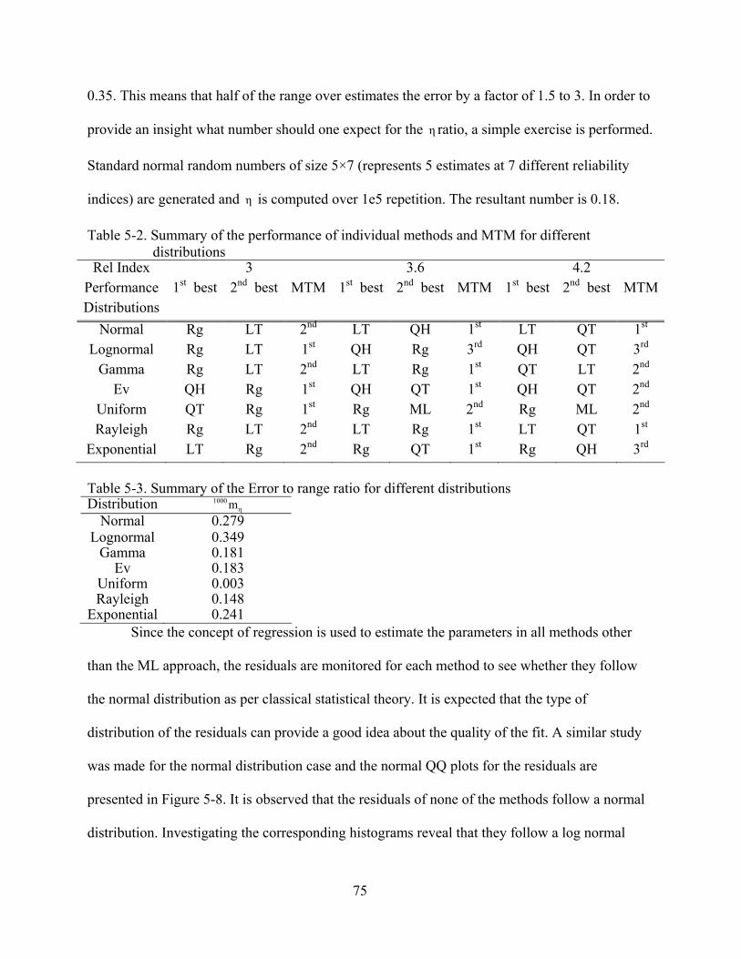
75

0.35. This means that half of the range over estimates the error by a factor of 1.5 to 3. In order to

provide an insight what number should one expect for the η ratio, a simple exercise is performed.

Standard normal random numbers of size 5×7 (represents 5 estimates at 7 different reliability

indices) are generated and η is computed over 1e5 repetition. The resultant number is 0.18.

Table 5-2. Summary of the performance of individual methods and MTM for different distributions

Rel Index 3 3.6 4.2 Performance 1st best 2nd best MTM 1st best 2nd best MTM 1st best 2nd best MTMDistributions

Normal Rg LT 2nd LT QH 1st LT QT 1st Lognormal Rg LT 1st QH Rg 3rd QH QT 3rd

Gamma Rg LT 2nd LT Rg 1st QT LT 2nd Ev QH Rg 1st QH QT 1st QH QT 2nd

Uniform QT Rg 1st Rg ML 2nd Rg ML 2nd Rayleigh Rg LT 2nd LT Rg 1st LT QT 1st

Exponential LT Rg 2nd Rg QT 1st Rg QH 3rd Table 5-3. Summary of the Error to range ratio for different distributions Distribution 1000

ηm Normal 0.279

Lognormal 0.349 Gamma 0.181

Ev 0.183 Uniform 0.003 Rayleigh 0.148

Exponential 0.241 Since the concept of regression is used to estimate the parameters in all methods other

than the ML approach, the residuals are monitored for each method to see whether they follow

the normal distribution as per classical statistical theory. It is expected that the type of

distribution of the residuals can provide a good idea about the quality of the fit. A similar study

was made for the normal distribution case and the normal QQ plots for the residuals are

presented in Figure 5-8. It is observed that the residuals of none of the methods follow a normal

distribution. Investigating the corresponding histograms reveal that they follow a log normal

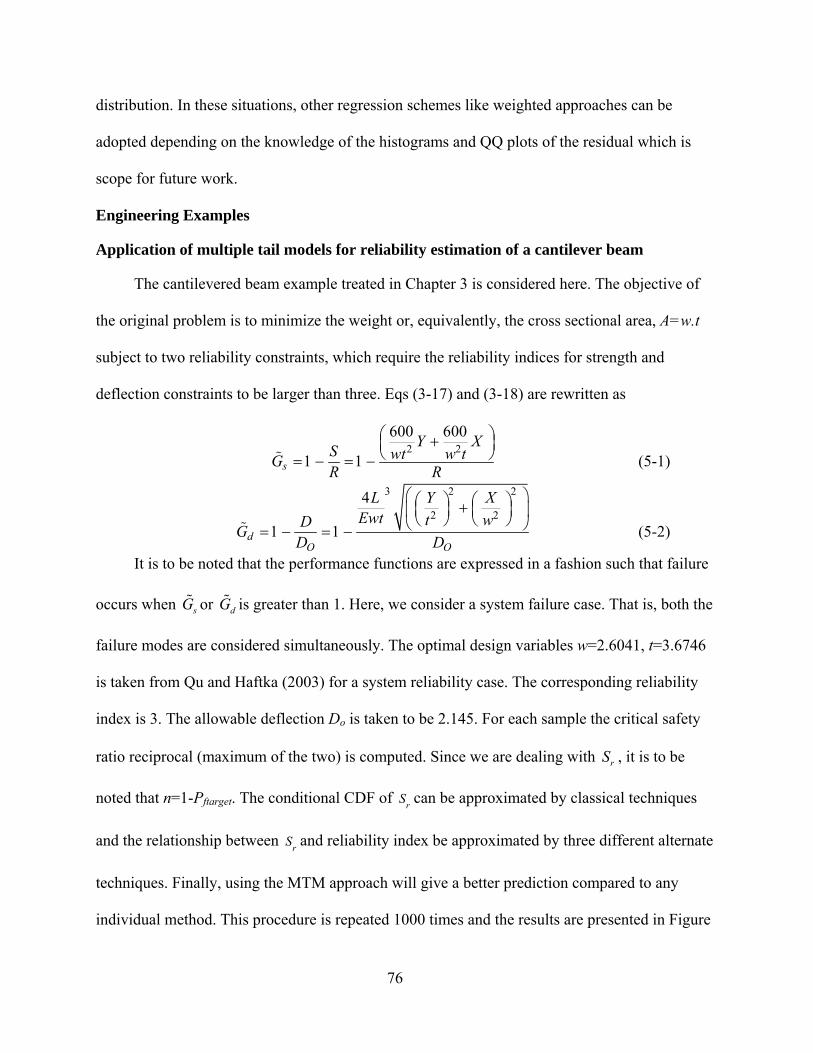
76

distribution. In these situations, other regression schemes like weighted approaches can be

adopted depending on the knowledge of the histograms and QQ plots of the residual which is

scope for future work.

Engineering Examples

Application of multiple tail models for reliability estimation of a cantilever beam

The cantilevered beam example treated in Chapter 3 is considered here. The objective of

the original problem is to minimize the weight or, equivalently, the cross sectional area, A=w.t

subject to two reliability constraints, which require the reliability indices for strength and

deflection constraints to be larger than three. Eqs (3-17) and (3-18) are rewritten as

s

Y XS wt w tGR R

2 2600 600⎛ ⎞+⎜ ⎟

⎝ ⎠= 1− = 1− (5-1)

dO O

L Y XEwt t wDG

D D

3 2 2

2 2

⎛ ⎞4 ⎛ ⎞ ⎛ ⎞+⎜ ⎟ ⎜ ⎟⎜ ⎟⎝ ⎠ ⎝ ⎠⎝ ⎠= 1− = 1− (5-2)

It is to be noted that the performance functions are expressed in a fashion such that failure

occurs when sG or dG is greater than 1. Here, we consider a system failure case. That is, both the

failure modes are considered simultaneously. The optimal design variables w=2.6041, t=3.6746

is taken from Qu and Haftka (2003) for a system reliability case. The corresponding reliability

index is 3. The allowable deflection Do is taken to be 2.145. For each sample the critical safety

ratio reciprocal (maximum of the two) is computed. Since we are dealing with rS , it is to be

noted that n=1-Pftarget. The conditional CDF of rS can be approximated by classical techniques

and the relationship between rS and reliability index be approximated by three different alternate

techniques. Finally, using the MTM approach will give a better prediction compared to any

individual method. This procedure is repeated 1000 times and the results are presented in Figure

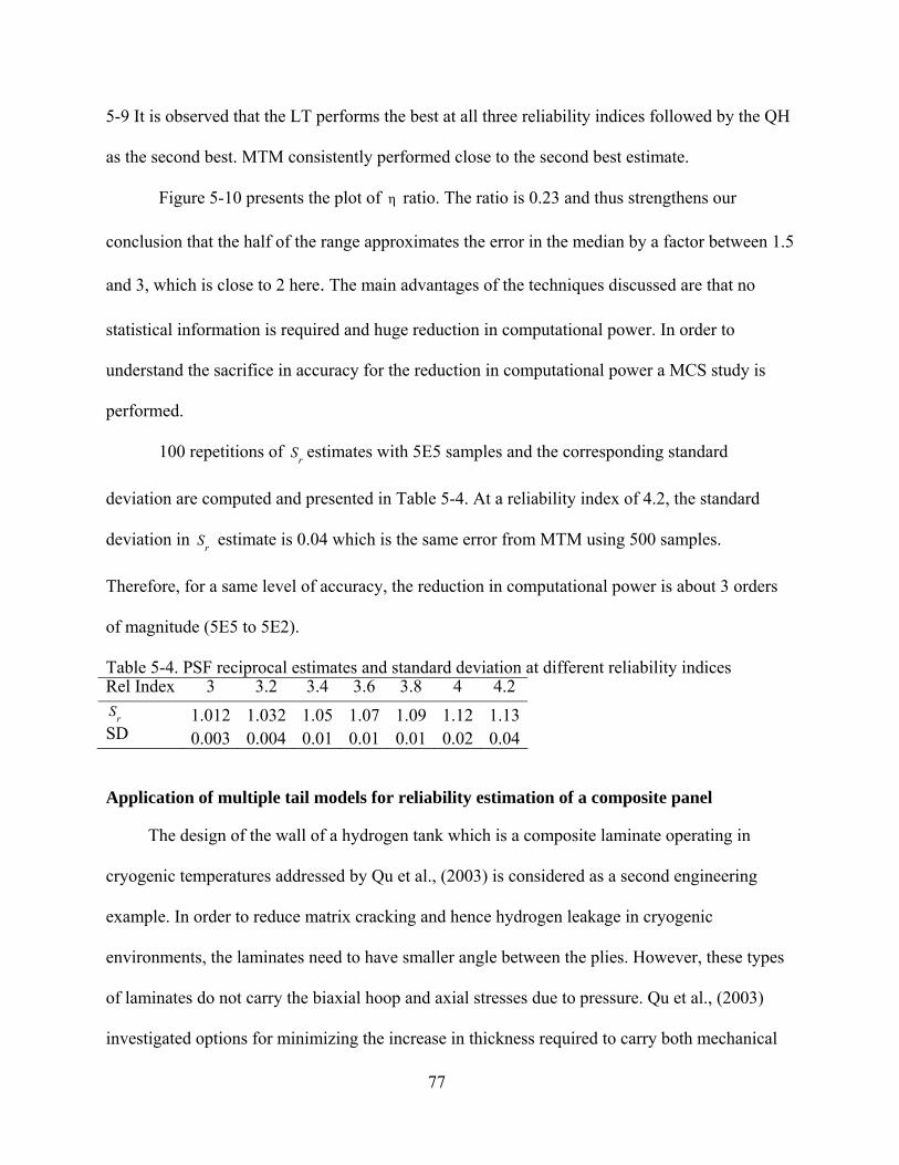
77

5-9 It is observed that the LT performs the best at all three reliability indices followed by the QH

as the second best. MTM consistently performed close to the second best estimate.

Figure 5-10 presents the plot of η ratio. The ratio is 0.23 and thus strengthens our

conclusion that the half of the range approximates the error in the median by a factor between 1.5

and 3, which is close to 2 here. The main advantages of the techniques discussed are that no

statistical information is required and huge reduction in computational power. In order to

understand the sacrifice in accuracy for the reduction in computational power a MCS study is

performed.

100 repetitions of rS estimates with 5E5 samples and the corresponding standard

deviation are computed and presented in Table 5-4. At a reliability index of 4.2, the standard

deviation in rS estimate is 0.04 which is the same error from MTM using 500 samples.

Therefore, for a same level of accuracy, the reduction in computational power is about 3 orders

of magnitude (5E5 to 5E2).

Table 5-4. PSF reciprocal estimates and standard deviation at different reliability indices Rel Index 3 3.2 3.4 3.6 3.8 4 4.2

rS 1.012 1.032 1.05 1.07 1.09 1.12 1.13SD 0.003 0.004 0.01 0.01 0.01 0.02 0.04

Application of multiple tail models for reliability estimation of a composite panel

The design of the wall of a hydrogen tank which is a composite laminate operating in

cryogenic temperatures addressed by Qu et al., (2003) is considered as a second engineering

example. In order to reduce matrix cracking and hence hydrogen leakage in cryogenic

environments, the laminates need to have smaller angle between the plies. However, these types

of laminates do not carry the biaxial hoop and axial stresses due to pressure. Qu et al., (2003)

investigated options for minimizing the increase in thickness required to carry both mechanical

78

and thermal residual strains. The geometry and loading conditions of the problem is presented in

Figure 5-11. The laminate is subject to mechanical (Nx and Ny) load and thermal loading due to

operating temperature -423oF where the stress free temperature is 300oF. The objective of the

actual problem was to optimize the weight of laminate with two ply angles [ ]1 2,θ θ± ± . The ply

angles and ply thickness ( 1 2 and t t ) are the design variables. The material used is IM600/133

graphite epoxy of ply thickness 0.005 inch. Qu et al., (2003) performed the deterministic design

optimization using continuous design variables. In order to account for the uncertainties and

make the deterministic optimal design comparable to probabilistic optimal design, they used a

safety factor of 1.4. For further details, the reader is referred to Qu et al., (2003). The mechanical

properties are presented in Table 5-5.

The deterministic optimization problem is formulated as

1 2

1 2

1 1 1 2 2 2 12 12

Minimize 4( )Such that , 0.005

, , L U L U UF F F

h t tt t

S S Sε ε ε ε ε ε γ γ

= +≥

≤ ≤ ≤ ≤ ≤

(5-3)

All material properties are assumed to be random, uncorrelated and follow normal

distributions. The coefficient of variation is presented in Table 5-6. Here, thickness is in inches

and h is the laminate thickness. Superscripts U and L represent upper and lower limits of the

associated quantities. 1 2 12, , and ε ε γ are the ply strains along fiber direction, transverse to fiber

direction, and shear strain, respectively. 2 12 1 2, , and E G α α are functions of temperature. Qu et al

(2001) show that at 20.2K (-423 ˚ F) the thickness of the optimum laminates obtained by using

temperature dependent material properties is 80% less than that using constant material

properties at 298 K (77˚ F ). Qu et al (2003) observed that 2Uε is the active constraint. For a

feasible design, 21 different temperatures uniformly distributed between 20oK and 300oK is

79

considered and the strain constraints are applied to these temperatures. The mean is computed at

a particular temperature and random numbers generated based on coefficient of variation. The

mean for other parameters are presented in Table 5-7. The deterministic optimal design obtained

by Qu et al (2003) is presented in Table 5-8.

The transverse strain on the first ply (direction 2) is the critical strain. The limit state is

defined as the difference between the critical strain and the upper bound of the allowable strain.

2 1UG ε ε= − (5-4)

Failure is said to occur if Eq. (5-4)> 0. In order to extend this example for demonstrating the

multiple tail models approach, the second optimal design in Table 5-8 is considered. The loads

are increased by a factor of 1.1 (Nx -5280 lb/inch and Ny -2640 lb/inch) so that the failure

probability is of the order of 1e-3.

500 random critical strain values are generated. Similar to the previous examples, 5

different techniques are used to fit the tail of the response distribution. The results are presented

in Figures 5-12 and 5-13. As observed in other examples the MTM compared at least close to the

second best in estimates from individual methods. However, the ratio of mean error to mean

range is 0.22 which means that half of the range overestimates the error by a factor of around

2.which falls within the range of 1.5 and 3 that was observed earlier in section. The 1e7 sample

based PSF reciprocal estimation and the corresponding standard deviation is presented in Table

5-9. At reliability index of 4.2, it is seen that the standard deviation is 0.0063 and the multiple

tail model provides an estimate with an error of 0.05 which is off by a factor of 8. The number of

samples used for this estimation is 500, which is about 4 orders of magnitude less than 1e7 Due

to the prohibitive computational power required, an exercise similar to the previous example is

80

not performed here. Instead the estimate from 500 samples and 1e7 samples are compared

directly.

Table 5-5. Mechanical properties of the composite laminates Elastic properties 1 2 12 12, , and E E G ν Coefficients of thermal expansion

1 2 and α α

Stress-free temperature zeroT Failure strains 1 1 2 2 12, , , and L U L U Uε ε ε ε γ Safety factor FS Table 5-6: Coefficient of variation for random material properties

1 2 12 12, , ,E E G ν 1 2,α α zeroT 1 1,L Uε ε 2 2 12, ,L U Uε ε γ 0.035 0.035 0.03 0.06 0.09 Table 5-7: Mean of random variables

1E 12ν zeroT 1Lε 1

Uε 2Lε 2

Uε 12Uγ

21.5x106 0.359 300 -0.0109 0.0103 -0.013 0.0154 0.0138 Table 5-8: Deterministic optima found by Qu et al (2003) θ1 (deg) θ2 (deg) t1 (in) t2 (in) h (in) 0.00 28.16 0.005 0.02 0.1 27.04 27.04 0.01 0.015 0.1 25.16 27.31 0.005 0.020 0.1

Table 5-9: Composite laminate. rS reciprocal estimates and standard deviation at different

reliability indices Rel Index 3 3.2 3.4 3.6 3.8 4 4.2

1E+07 1.0043 1.0304 1.0579 1.0862 1.1157 1.1480 1.1824 SD 0.0007 0.0009 0.0015 0.0021 0.0025 0.0046 0.0063

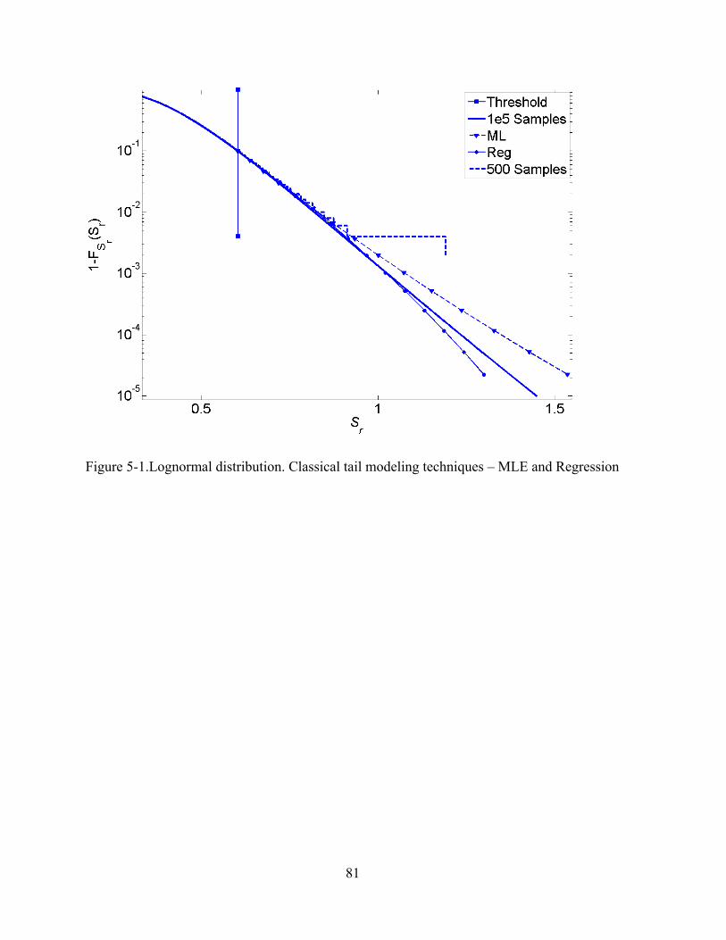
81

Figure 5-1.Lognormal distribution. Classical tail modeling techniques – MLE and Regression

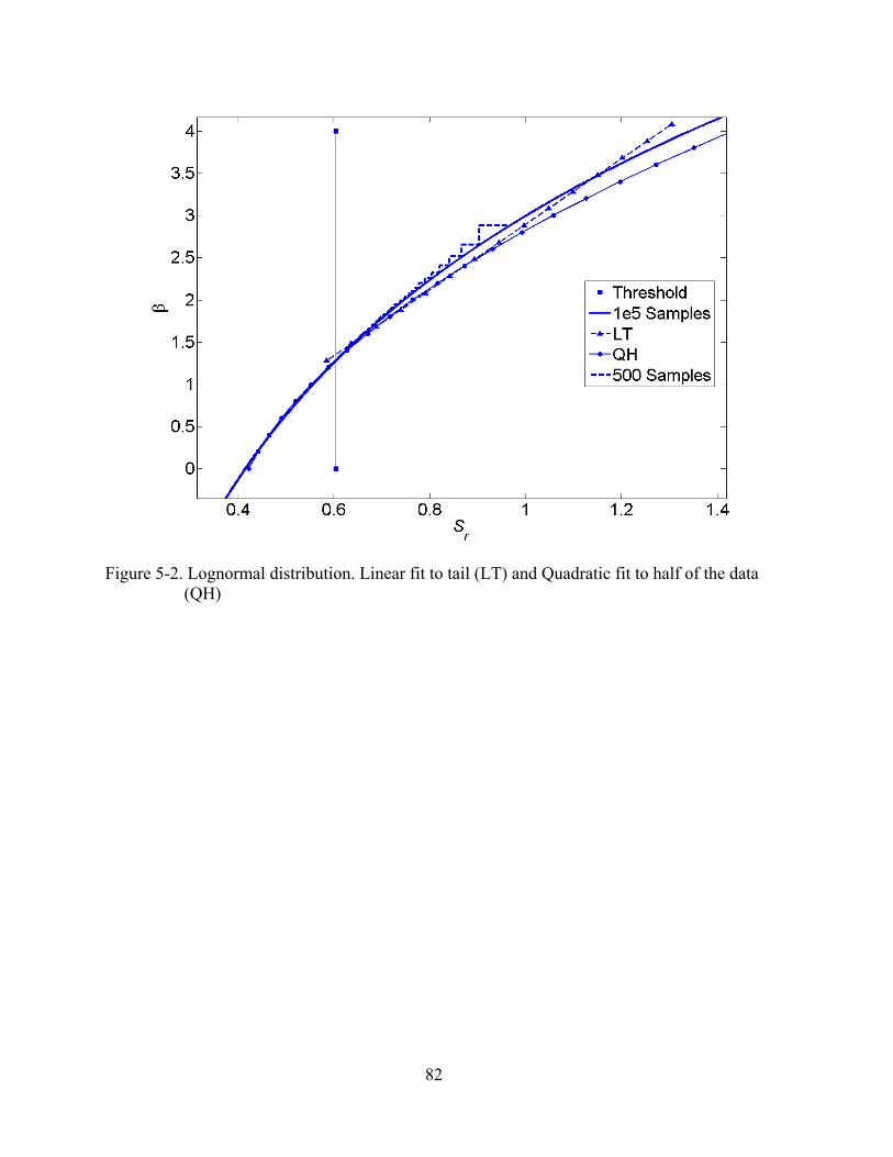
82

Figure 5-2. Lognormal distribution. Linear fit to tail (LT) and Quadratic fit to half of the data (QH)

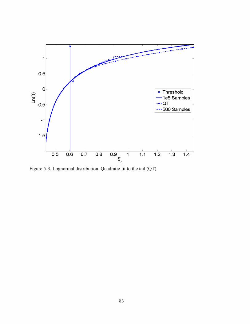
83

Figure 5-3. Lognormal distribution. Quadratic fit to the tail (QT)

84

Figure 5-4.Lognormal distribution. Multiple tail models

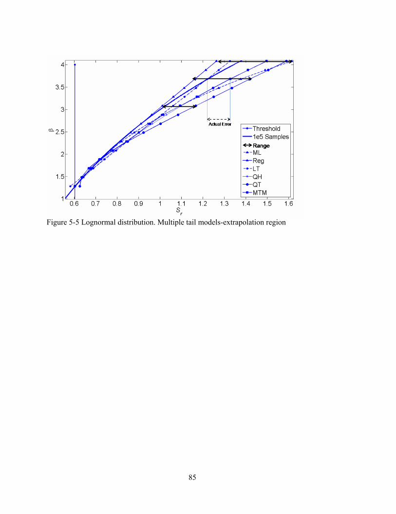
85

Figure 5-5 Lognormal distribution. Multiple tail models-extrapolation region

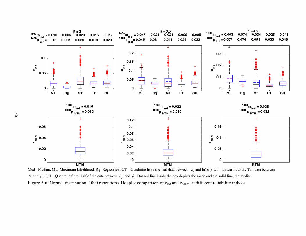
86

Med= Median. ML=Maximum Likelihood, Rg- Regression, QT – Quadratic fit to the Tail data between rS and ln( β ), LT – Linear fit to the Tail data between

rS and β , QH – Quadratic fit to Half of the data between rS and β . Dashed line inside the box depicts the mean and the solid line, the median.

Figure 5-6. Normal distribution. 1000 repetitions. Boxplot comparison of eind and eMTM at different reliability indices

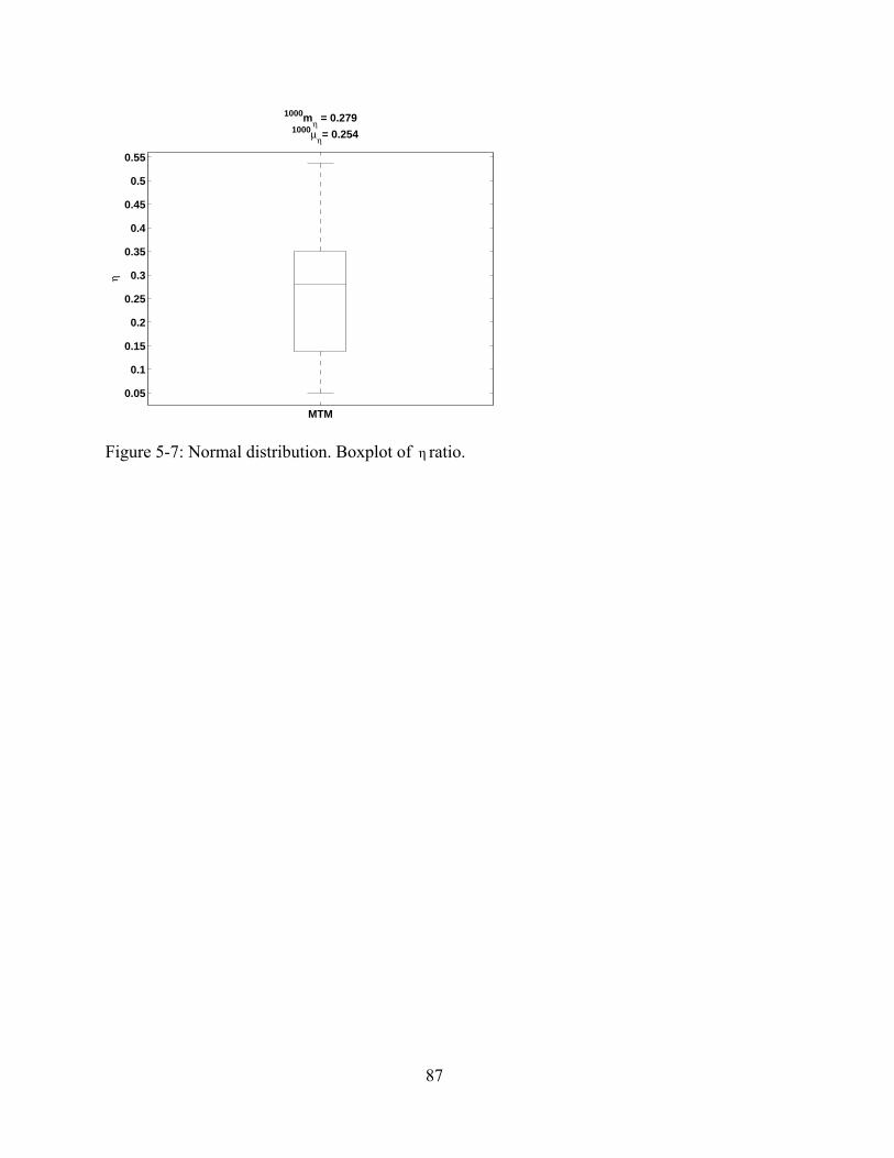
87

MTM

0.05

0.1

0.15

0.2

0.25

0.3

0.35

0.4

0.45

0.5

0.55

η1000mη = 0.279

1000μη= 0.254

Figure 5-7: Normal distribution. Boxplot of η ratio.

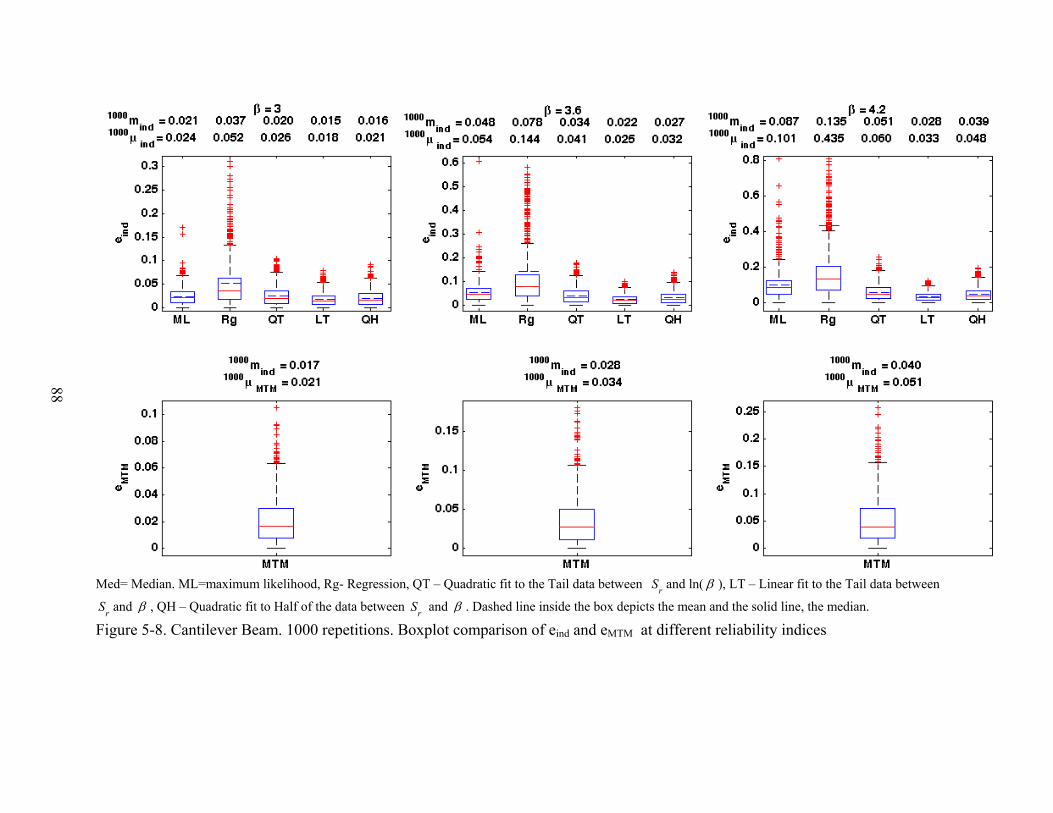
88

Med= Median. ML=maximum likelihood, Rg- Regression, QT – Quadratic fit to the Tail data between rS and ln( β ), LT – Linear fit to the Tail data between

rS and β , QH – Quadratic fit to Half of the data between rS and β . Dashed line inside the box depicts the mean and the solid line, the median.

Figure 5-8. Cantilever Beam. 1000 repetitions. Boxplot comparison of eind and eMTM at different reliability indices

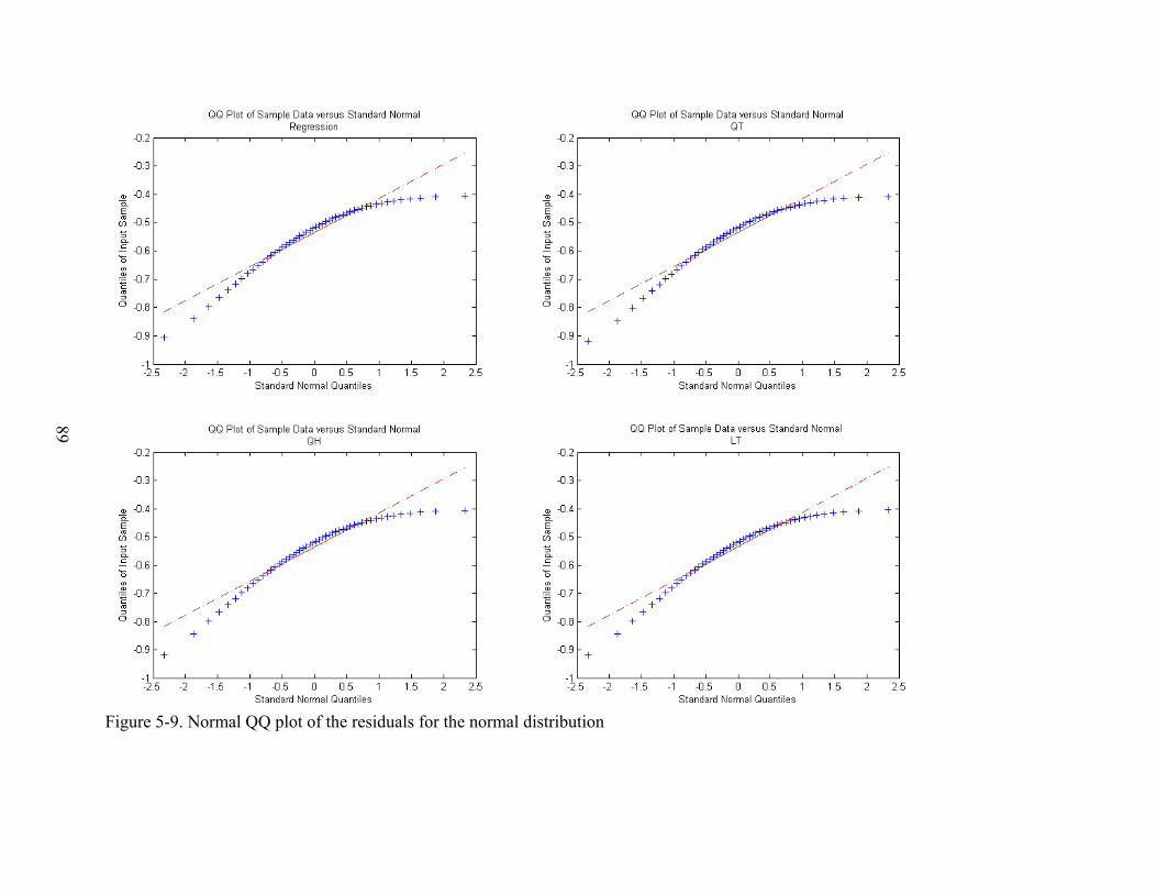
89

Figure 5-9. Normal QQ plot of the residuals for the normal distribution

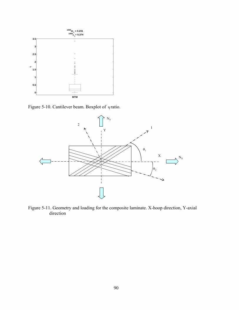
90

MTM

0

0.5

1

1.5

2

2.5

3

3.5

η1000mη = 0.231

1000μη= 0.374

Figure 5-10. Cantilever beam. Boxplot of η ratio.

NX

θ2

X

Y1

2

θ1

NY

NX

θ2

X

Y1

2

θ1

NY

Figure 5-11. Geometry and loading for the composite laminate. X-hoop direction, Y-axial direction

91

ML=Maximum Likelihood, Rg- Regression, QT – Quadratic fit to the Tail data between rS and ln( β ), LT – Linear fit to the Tail data between rS and β , QH – Quadratic fit to half of the data between rS and β .Dashed line inside the box depicts the mean and the solid line, the median Figure 5-12. Composite laminate of cryogenic tank. 1000 repetitions. Boxplot comparison of eind and eMTM at different reliability

indices...

92

MTM

0

0.5

1

1.5

2

2.5

3η

1000mη = 0.220

1000μη= 0.356

Figure 5-13. Composite laminate of cryogenic tank. Boxplot of η ratio.

93

CHAPTER 6 CONCLUSIONS

High reliability estimations with expensive computer models pose a challenge because of

the high computational expense. Extrapolating into higher reliability indices with information

from lower reliability indices can be one solution to this problem. In order to do this, the tails of

the distribution are to be modeled well. Inverse reliability measures feature several advantages

and is widely used by researchers in structural reliability. This work explores the usefulness of

inverse measures in tail modeling. Two classical tail modeling techniques were discussed.Three

extrapolation techniques that can complement the classical tail modeling techniques were

developed. This work proposes to use a multiple tail model approach in which all the five

techniques are applied simultaneously to estimate the inverse measure, and the median is taken

to be the best estimate. It is shown that the range of the five methods can be utilized to

approximate the error associated with the estimate. The proposed method was demonstrated on

seven statistical distributions and engineering examples. It was shown that the sacrifice in

accuracy compared to the crude MCS is relatively small compared to the immense reduction in

computational power.

94

APPENDIX A PSF ESTIMATION FOR A SYSTEM RELIABILITY

The estimation of PSF for a system reliability case is demonstrated with an example. This

example is artificial and is an illustration of a case with multiple limit state functions. The

example is presented in Figure A1.The limit state functions are:

3 2

115

40x xG y

⎛ ⎞− += −⎜ ⎟

⎝ ⎠ (A1)

2 2

2( 5) ( 12) 0.8

30 140x y x yG

⎛ ⎞+ − − −= + −⎜ ⎟⎝ ⎠

(A2)

380 20G yx

⎛ ⎞= − −⎜ ⎟⎝ ⎠

(A3)

The limit states are functions of two random variables x and y. The distributions of the random

variables are presented in Table A-1. The example has been created in such a fashion that each

limit state and its intersection with other limit states contributes significantly to the total failure.

It should be noted that non linear functions are used to emphasize the advantage of using MCS

and a PSFbased approach to estimate failure probability. Using FORM in these circumstances

might introduce huge error due to linearizing the limit state function at the most probable point

of failure. The contributions of failure modes to the total failure are listed in Table A-2. The

system PSF can be estimated as described in the flowchart in Figure A-1. The limit states are

functions of two random variables x and y. The PSF estimated for different target failure

probabilities are listed in Table A-3. For a target failure probability of 0.557 which is the actual

failure probability as listed in Table A-3, the PSF is estimated as 1. When a lower target failure

probability of 0.5 is used, the PSF is estimated to be 0.844 indicating that the system is unsafe

and when a larger target failure probability of 0.6 is used, the PSF is found to be 1.12 showing

that the system is over safe. This shows that PSF based approach can adequately address system

reliability case accounting for the interactions between the modes.

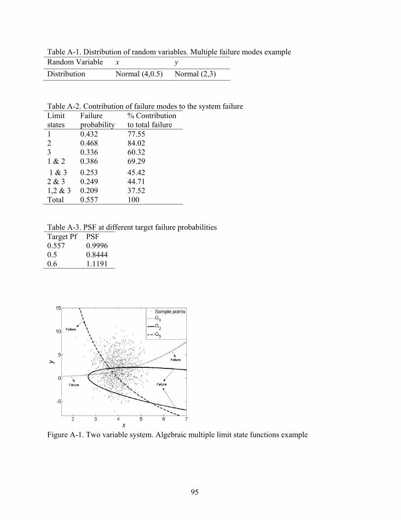
95

Table A-1. Distribution of random variables. Multiple failure modes example

Table A-2. Contribution of failure modes to the system failure Limit states

Failure probability

% Contribution to total failure

1 0.432 77.55 2 0.468 84.02 3 0.336 60.32 1 & 2 0.386 69.29 1 & 3 0.253 45.42 2 & 3 0.249 44.71 1,2 & 3 0.209 37.52 Total 0.557 100 Table A-3. PSF at different target failure probabilities Target Pf PSF 0.557 0.9996 0.5 0.8444 0.6 1.1191

Figure A-1. Two variable system. Algebraic multiple limit state functions example

Random Variable x y Distribution Normal (4,0.5) Normal (2,3)

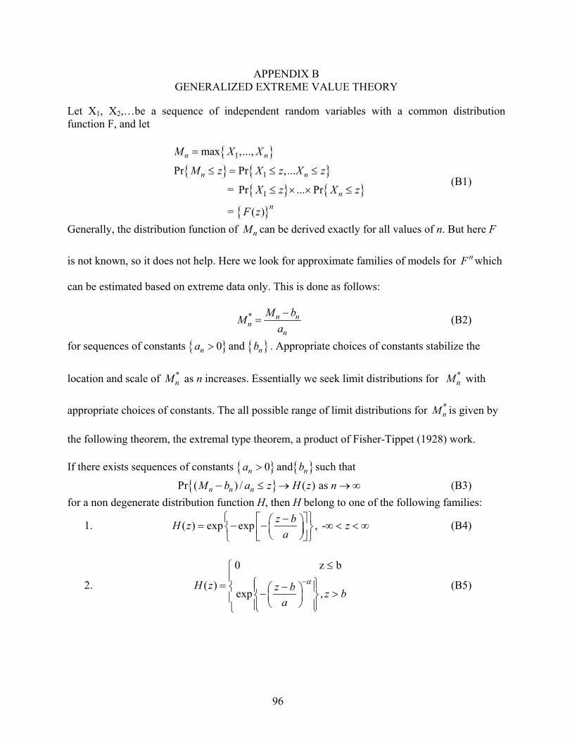
96

APPENDIX B GENERALIZED EXTREME VALUE THEORY

Let X1, X2,…be a sequence of independent random variables with a common distribution function F, and let

{ }{ } { }

{ } { }{ }

1

1

1

max ,...,

Pr Pr ,...

= Pr ... Pr

= ( )

n n

n n

nn

M X X

M z X z X z

X z X z

F z

=

≤ = ≤ ≤

≤ × × ≤ (B1)

Generally, the distribution function of nM can be derived exactly for all values of n. But here F

is not known, so it does not help. Here we look for approximate families of models for nF which

can be estimated based on extreme data only. This is done as follows:

* n nn

n

M bMa−

= (B2)

for sequences of constants { }0na > and { }nb . Appropriate choices of constants stabilize the

location and scale of *nM as n increases. Essentially we seek limit distributions for *

nM with

appropriate choices of constants. The all possible range of limit distributions for *nM is given by

the following theorem, the extremal type theorem, a product of Fisher-Tippet (1928) work.

If there exists sequences of constants { }0na > and{ }nb such that

{ }Pr ( ) / ( ) as n n nM b a z H z n− ≤ → →∞ (B3) for a non degenerate distribution function H, then H belong to one of the following families:

1. ( ) exp exp , -z bH z za

⎧ ⎫−⎡ ⎤⎛ ⎞= − − ∞ < < ∞⎨ ⎬⎜ ⎟⎢ ⎥⎝ ⎠⎣ ⎦⎩ ⎭ (B4)

2.

0 z b

( )exp ,

H z z b z ba

α−

≤⎧⎪ ⎧ ⎫= −⎪ ⎪⎨ ⎛ ⎞− >⎨ ⎬⎜ ⎟⎪ ⎝ ⎠⎪ ⎪⎩ ⎭⎩

(B5)

97

3. exp , ,

( )

1 z b,

z b z bH z a

α⎧ ⎧ ⎫⎡ ⎤−⎪ ⎪⎛ ⎞⎪ − − <⎢ ⎥⎪ ⎨ ⎬⎜ ⎟= ⎝ ⎠⎨ ⎢ ⎥⎪ ⎪⎣ ⎦⎩ ⎭⎪≥⎪⎩

(B6)

Here, a and b are the scale and location parameters. α is the shape parameter. These three classes

of distributions are called the extreme value distributions with types I, II and III, widely known

as Gumbel, Frechet and Weibull families respectively. The above theorem implies that the

normalized maxima have a limiting distribution that must be one of the three types of extreme

value distribution. The three families of distributions can be combined into a single family of

models having distribution function of the form

1/

( ) exp 1 zH zξμξ

σ

−⎧ ⎫−⎡ ⎤⎪ ⎪⎛ ⎞= − +⎨ ⎬⎜ ⎟⎢ ⎥⎝ ⎠⎣ ⎦⎪ ⎪⎩ ⎭ (B7)

such that { }:1 ( ) / 0z zξ μ σ+ − > , where the parameters satisfy μ−∞ < < ∞ , 0σ > and

ξ−∞ < < ∞ . This is the generalized extreme value (GEV) family of distributions. Here, μ is the

location parameter, σ is the scale parameter, ξ is the shape parameter. Type II and III families

correspond to 0ξ > and 0ξ < cases in (9). 0ξ = can be interpreted as the Gumbel family with

distribution function:

( ) exp exp zH z μσ

⎡ ⎤−⎧ ⎫⎛ ⎞= − −⎨ ⎬⎜ ⎟⎢ ⎥⎝ ⎠⎩ ⎭⎣ ⎦ (B8)

98

APPENDIX C MAXIMUM LIKELIHOOD ESTIMATION

The PDF of the Pareto Distribution is given by:

111 1 0( )

1 = 0

i

z

z

f x

e

ξ

σ

ξ ξσ σ

ξσ

⎛ ⎞− +⎜ ⎟⎝ ⎠

−

⎧⎧ ⎫⎪ + ≠⎨ ⎬⎪ ⎩ ⎭= ⎨

⎪⎪⎩

(C1)

Here, the z represents the exceedances. ξ and σ are the shape and scale parameters respectively.

The likelihood function for a sample of z1…zn of iid GP random variables is given by:

( )

11

11

1

1 1 0, ,

1 = 0

n

ini

in

ni

zL z

e

ξ

σ

ξ ξσσξ σ

ξσ

⎛ ⎞− +⎜ ⎟⎝ ⎠

=

−

=

⎧⎛ ⎞⎪ + ≠⎜ ⎟⎪⎪ ⎝ ⎠= ⎨

⎪⎪⎪⎩

∏

∏ (C2)

The log likelihood function is expressed as:

1

1

1log 1 log 1 1+ 0log ( , )

1log = 0

ni

ii

n

ii

zn zL

n z

ξξσξ σ σ

ξ σσ ξ

σ

=

=

⎧ ⎛ ⎞ ⎛ ⎞− − + + >⎪ ⎜ ⎟⎜ ⎟⎝ ⎠⎝ ⎠⎪= ⎨

⎪− −⎪⎩

∑

∑ (C3)

The maximization of (C3) is best made by reparametrization:

( ) ( ), ,σ ξ τ ξ→ with ξτσ

=

yielding

( ) ( )1

1log , log 1 log 1n

ii

h L n zξτ ξ ττ ξ =

⎛ ⎞⎛ ⎞= = − − + +⎜ ⎟ ⎜ ⎟⎝ ⎠ ⎝ ⎠

∑ (C4)

( )1

1log log 1 log 1n

ii

n n zξ τ τξ =

⎛ ⎞= − + − + +⎜ ⎟

⎝ ⎠∑ (C5)

The max of (C5) is found as the minimum of the negative of(C5). The MLE are given by

differentiating (C5) and equating to zero.

99

21

1 ˆlog(1 ) 0ˆ ˆn

ii

h n zτξ ξ ξ =

∂= − + + =

∂ ∑ (C6)

1

1 11 0ˆ ˆ ˆ1

n

iii

h n zzτ τ τ τ=

∂ ⎛ ⎞= + + =⎜ ⎟∂ +⎝ ⎠∑ (C7)

(C6) yields 1

1ˆ ˆlog(1 )n

ii

zn

ξ τ=

= +∑ and (C7)can be solved for τ̂ . Numerical techniques are used for

the maximization of h in (C5) using algorithms that are available in standard software packages.

In most situations estimation is done using iid samples. In such cases, the interst is to

determine the behavior of the estimator as a sample size ∞ . This is referred to as asymptotic

behavior. Under certain regularity conditions like: the first and second derivatives of the log

likelihood function must be defined., the fisher information matrix must not be equal to zero,

MLEs exhibit following properties

• Asymptotically unbiased (i.e.,) its bias tends to zero as the number of samples increases to infinity.

• MLE is asymptotically guassian. That is, as sample increases the distribution of MLE tends to normal distribution. Here, the covariance matrix can be obtained as the inverse of the fisher information matrix.

100

APPENDIX D ERROR ANALYSIS FOR GPD

This appendix describes the error analysis for the probability content estimated using tail

modeling. When the distribution of exceedance is approximated using GPD, there are two

sources of error:

1. Modelling error

2. Sampling component of the total error

The modelling error refers to the capacity of the GPD model to accurately represent the

distribution of exceedance data or the tail of the CDF. If the exact CDF is available, the CDF

estimated through GPD can be compared and the resulting error is the modeling error.

Depending on the empirical CDF, the GP fit will vary. This introduces sampling error. The

sampling error comes from the fact that the GPD parameters vary depending on the exceedance.

The input variables generally come from sampling distributions like the LHS or any other

suitable DOE. Depending on these sampling points, the threshold differs. Hence, the exceedance

is affected and therefore the estimated parameters and eventually the fitted GPD.

If we have the privilege to generate large number of samples and use a fraction of it as

exceedance data to fit a GPD, the estimated parameters in the process can be considered as

‘optimal’ parameters since they are based on a large sample size. These parameters can be used

to estimate probability contents at certain levels and can be compared with the probability

content estimated by a GPD with small sample size. This difference will dictate the sampling

error contribution to the total error.

In an attempt to study the modeling and sampling error, an example problem is treated

here. The example under investigation is Y =exp(x) and x~N(0,1). The modeling error is studied

comparing the estimated probability content using a GPD with a large sample size and the exact

101

probability content generated by analytical expression of the lognormal distribution. The

parameters for the GPD are obtained by MLE method.

Let the conditional CDF ( )/P Y u z Y u> + > be represented by ( )uF z . In this example, it

is possible to estimate this quantity exactly. Using extreme value theory for exceedances,

( )uF z can be approximated by a GP distribution denoted by ,ˆ ( )F zξ σ . Let the estimated CDF be

denoted by $,

ˆ ( )F zξ σ . Let the GPD which is based on the optimal parameters be denoted

by *,

ˆ ( )F zξ σ .

1e6 samples based on LHS design are generated. The Y’s are sorted

as: (1) (2) (1 6).... eY Y Y≤ ≤ ≤ . This is called the order statistics of Y. Choosing the appropriate ‘u’,

the threshold value is very critical. u defines the beginning of the upper tail. The uF is chosen to

be 0.90 and the corresponding value of Y is chosen as u. Once u is chosen, the exceedance data

is formed and the ML estimates are obtained for the parameters. These estimates are used to

estimate the probability content at different levels of Y. The results are presented in Table D-1.

Five repetitions of 1e6 samples are used for each level. The mean and standard deviation of the

CDF estimates based on GPD are presented. The error refers to the total error in percentage. The

sampling error component of the total error is extracted using estimated optimal parameters. The

optimal parameters were obtained based on a million samples. Here, 3 percent of the data was

considered as exceedance. The results are presented in Table D- 2. From Tables D-1 and D-2, it

can be clearly seen that the sampling error is high compared to the modeling error. So, if we can

account for the sampling errors, tail modeling has a fairly good capacity to model the tails of the

distribution to estimate probability contents.

102

TableD-1. Modelling error ( ( )gF z - *,

ˆ ( )F zξ σ ). The standard deviation is very low that it is not presented.

TableD-2: Sampling error ( *,

ˆ ( )F zξ σ - $,

ˆ ( )F zξ σ )

Y Exact ( )gF z GPD *,

ˆ ( )F zξ σΑ Error%

4 0.08283 0.07988 3.56 5 0.05376 0.05299 1.43 6 0.03659 0.03647 0.33 7 0.02583 0.02587 -0.16 8 0.01879 0.01884 -0.28 9 0.01400 0.01403 -0.19 10 0.01065 0.01065 0.00 11 0.00824 0.00822 0.24 12 0.00648 0.00645 0.49

Y GPD- 1e6 samples *,

ˆ ( )F zξ σΑ GPD- 1e2 samples $

,ˆ ( )F zξ σ Error

% 4 0.07988 0.08710 -9.04 5 0.05299 0.05797 -9.39 6 0.03647 0.03997 -9.61 7 0.02587 0.02824 -9.15 8 0.01884 0.02039 -8.20 9 0.01403 0.01503 -7.17 10 0.01065 0.01135 -6.53 11 0.00822 0.00877 -6.69 12 0.00645 0.00696 -7.95

103

APPENDIX E ACCURACY AND CONVERGENCE STUDIES FOR NORMAL AND LOGNORMAL

DISTRIBUTIONS

The quantile of a probability distribution can be estimated using Eq.(4-8). The quantile2

can be related to the inverse measure in the structural reliability context where the probability

content is expressed as the target failure probability. Due to the various advantages of using

inverse measures in RBDO, we are interested in estimating them using tail modeling approach.

Here, we study the accuracy of the tail model to capture the quantile in the tails of the normal

distribution. In the following simulation study a y=x example where x ~N (0, 1) is treated. The

error metrics that are monitored are:

a) Bias error: Bias( )=Ep p px x x⎡ ⎤−⎣ ⎦ (E1)

1

1 Ns

p pi

x xNsim =

= −∑ (E2)

where,

: Estimated quantile

: Actual quantile

: Number of simulations

p

p

x

x

Nsim

b) RMSE error:

2 2

1

1( ) ( )Ns

p p p pi

x x x xNs =

⎡ ⎤− = −⎣ ⎦ ∑ (E3)

Here, we set out to study the effects of the threshold value, the number of exceedance data

on the accuracy of the quantile estimate. For each threshold value, four different exceedances are

tested. Since the exceedances vary, the number of samples used in each case varies. The results

are presented in Table E-1.The overall capacity of the tail modeling approach to capture the

quantiles in the tails of the normal distribution seems to be pretty good. For all the four threshold

2 A p quantile of a random variable X is any value x such that Pr(X≤ xp) = p

104

values, the % Bias error for the 25 exceedance data seem to be very less compared to higher

exceedance data. But, it is to be noted that the corresponding %RMSE errors are high

emphasizing the fact that the estimates from low number of exceedance data could be highly

unreliable. 25 exceedance data is considered low to estimate quantiles. 50 to 100 data is

considered realistic and 200 ideal. It can be clearly observed that the accuracy of the % Bias

increases as the threshold increases for the

Table E-1. Accuracy of the tail modeling approach to estimate quantiles. Normal distribution y = x. x~N(0,1). 500 simulations. ML estimated parameters

% Bias % RMSE Fu Nex NS 0.999 0.9999 0.99999 0.999 0.9999 0.99999

25 125 -8 -9 -5 48 98 216 50 250 -6 -10 -14 22 34 46 100 500 -3 -7 -11 11 16 22

0.8

200 1000 -2.5 -7.3 -12.5 5.1 8.5 12.0 25 166 -6 -7 -2 37 81 211 50 333 -4 -8 -11 17 28 44 100 666 -2 -6 -10 8 13 18

0.85

200 1333 -2.1 -6.1 -10.6 4.1 6.9 9.8 25 250 -3 -2 3 25 51 107 50 500 -4 -7 -10 11 18 25 100 1000 -2.2 -5.7 -9.4 5.4 9.3 13.1

0.9

200 2000 -0.8 -3.5 -6.8 2.6 4.8 7.1 25 500 -3 -3 0 12 26 57 50 1000 -2 -4 -5 6 11 17 100 2000 -0.8 -2.5 -4.5 2.8 5.5 8.5

0.95

200 4000 -0.4 -2.4 -5.2 1.3 2.6 4.0 Fu – Threshold in the CDF. Nex – Number of exceedance data. NS- Number of total samples used. 0.999, 0.9999, 0.99999 Quantiles required to be estimated. For a threshold of 0.85 and Nex=100, the -2,-6,-10 % Bias error in quantile translates to -27.6, -139.9 and -524.12% error in probability content same number of exceedance data. The threshold values, number of exceedance data is dependent

on the level of target quantile we wish to estimate. It can be observed that for a quantile of 0.999,

reasonably low quantiles such as 0.8 perform well enough with 50 to 100 exceedance data, if 5%

bias error is allowable. For a 0.9999 quantile, a threshold of 0.9 with 100 exceedance data

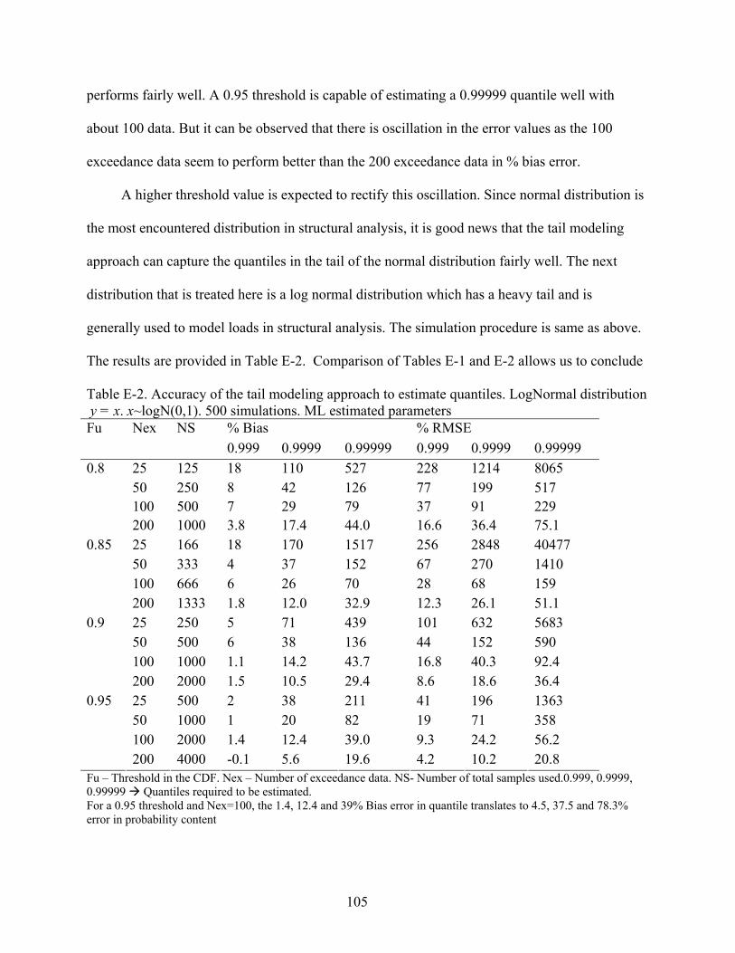
105

performs fairly well. A 0.95 threshold is capable of estimating a 0.99999 quantile well with

about 100 data. But it can be observed that there is oscillation in the error values as the 100

exceedance data seem to perform better than the 200 exceedance data in % bias error.

A higher threshold value is expected to rectify this oscillation. Since normal distribution is

the most encountered distribution in structural analysis, it is good news that the tail modeling

approach can capture the quantiles in the tail of the normal distribution fairly well. The next

distribution that is treated here is a log normal distribution which has a heavy tail and is

generally used to model loads in structural analysis. The simulation procedure is same as above.

The results are provided in Table E-2. Comparison of Tables E-1 and E-2 allows us to conclude

Table E-2. Accuracy of the tail modeling approach to estimate quantiles. LogNormal distribution y = x. x~logN(0,1). 500 simulations. ML estimated parameters

% Bias % RMSE Fu Nex NS 0.999 0.9999 0.99999 0.999 0.9999 0.99999

25 125 18 110 527 228 1214 8065 50 250 8 42 126 77 199 517 100 500 7 29 79 37 91 229

0.8

200 1000 3.8 17.4 44.0 16.6 36.4 75.1 25 166 18 170 1517 256 2848 40477 50 333 4 37 152 67 270 1410 100 666 6 26 70 28 68 159

0.85

200 1333 1.8 12.0 32.9 12.3 26.1 51.1 25 250 5 71 439 101 632 5683 50 500 6 38 136 44 152 590 100 1000 1.1 14.2 43.7 16.8 40.3 92.4

0.9

200 2000 1.5 10.5 29.4 8.6 18.6 36.4 25 500 2 38 211 41 196 1363 50 1000 1 20 82 19 71 358 100 2000 1.4 12.4 39.0 9.3 24.2 56.2

0.95

200 4000 -0.1 5.6 19.6 4.2 10.2 20.8 Fu – Threshold in the CDF. Nex – Number of exceedance data. NS- Number of total samples used.0.999, 0.9999, 0.99999 Quantiles required to be estimated. For a 0.95 threshold and Nex=100, the 1.4, 12.4 and 39% Bias error in quantile translates to 4.5, 37.5 and 78.3% error in probability content

106

that estimating quantiles in lognormal distribution is more challenging than normal distribution.

For a 0.999 quantile, 0.8 and 0.85 thresholds perform fairly well with 200 samples. Above a 0.9

threshold, 100 samples seem to render very good results. There is considerable difficulty in

estimating 0.9999 quantile with even a 100 exceedance data and a 0.95 threshold value. Needless

to mention, trying to estimate 0.99999 quantile deteriorates the accuracy of the estimation only.

In order to test whether higher threshold values enable us to estimate the extreme quantiles

accurately, simulation is conducted for threshold values ranging from 0.96 to 0.99 and results are

presented in Table E-3.

Table E-3. Accuracy of the tail modeling approach to estimate quantiles. Higher thresholds. LogNormal distribution

y = x. x~logN(0,1). 500 simulations. ML estimated parameters % Bias % RMSE Fu Nex NS

0.9999 0.99999 0.9999 0.9999925 625 50 254 171 958 50 1250 16 61 46 160

100 2500 9 30 18 42

0.96

200 5000 4 16 8 16 25 834 20 135 102 693 50 1667 12 49 35 98

100 3334 7 29 16 43

0.97

200 6667 3 13 6 12 25 1250 17 126 74 563 50 2500 6 29 19 49

100 5000 4 20 10 22

0.98

200 10000 1 8 4 8 25 2500 5 65 30 225 50 5000 2 19 10 25

100 10000 0.9 10 5 12

0.99

200 20000 0.2 6 2 5 Fu – Threshold in the CDF. Nex – Number of exceedance data. NS- Number of total samples used. 0.9999, 0.99999

Quantiles required to be estimated

Results from Table 4-3 clearly show that as the threshold is increased, the extreme quantiles are

also captured fairly well. With a 0.99 threshold and 100 exceedance data, we can achieve less

107

than one percent error in bias for estimating 0.9999 quantile. This requires 10000 samples.

Similarly the accuracy in estimating 0.99999 quantile is also better with 0.99 threshold and 200

exceedance data. A more accurate estimate can be expected if we raise the threshold to 0.999 or

higher.

108

APPENDIX F ACCURACY AND CONVERGENCE STUDIES FOR THE CANTILEVER BEAM

Stress Failure Mode

The stress failure mode for the cantilever beam discussed in Chapter 3 is considered here.

The optimal design variables w=2.4526; t=3.8884 for a target failure probability of 0.00125 (1e7

Samples) are adopted from (Qu and Haftka, 2004). The corresponding value of PSF for this

design is 1. For the optimal combination of the design variables, 500 samples based on the

distribution of the random variables are generated and the PSF is estimated for different

thresholds as discussed in Chapter 3. This procedure is repeated 100 times and the mean, 5%,

95% confidence intervals are estimated. The results are presented in Figure E-1. It can be

observed from the figure that the PSF estimated by regression approach is very unstable whereas

the median of PSF estimated by the ML approach is relatively stable. There is instability towards

higher threshold like 0.98 but the corresponding exceedance data are very less, which explains

the instability. The estimated mean of the PSF in the ML approach is close to 0.99 which is about

1% bias error in estimating the actual value of the PSF. The standard deviation of the PSF

estimate at a threshold of 0.9 with ML approach is about 0.003 which is 0.3% of the estimate.

The corresponding estimate of failure probability is 0.0011 with a standard deviation of 0.0001

which is about 10% of the estimate.

Deflection Failure Mode

The allowable deflection is chosen to be D0=2.25. Similar to the stress failure case, the

PSF is estimated at different thresholds for the optimal combination of the design variables. The

results are presented in Figure E-2. At a threshold of 0.9 and ML approach, the PSF is estimated

to be 0.99 with a standard deviation of 0.004. The corresponding failure probability estimate is

0.0013 with a standard deviation of 0.0001 which is about 8% of the estimate itself.

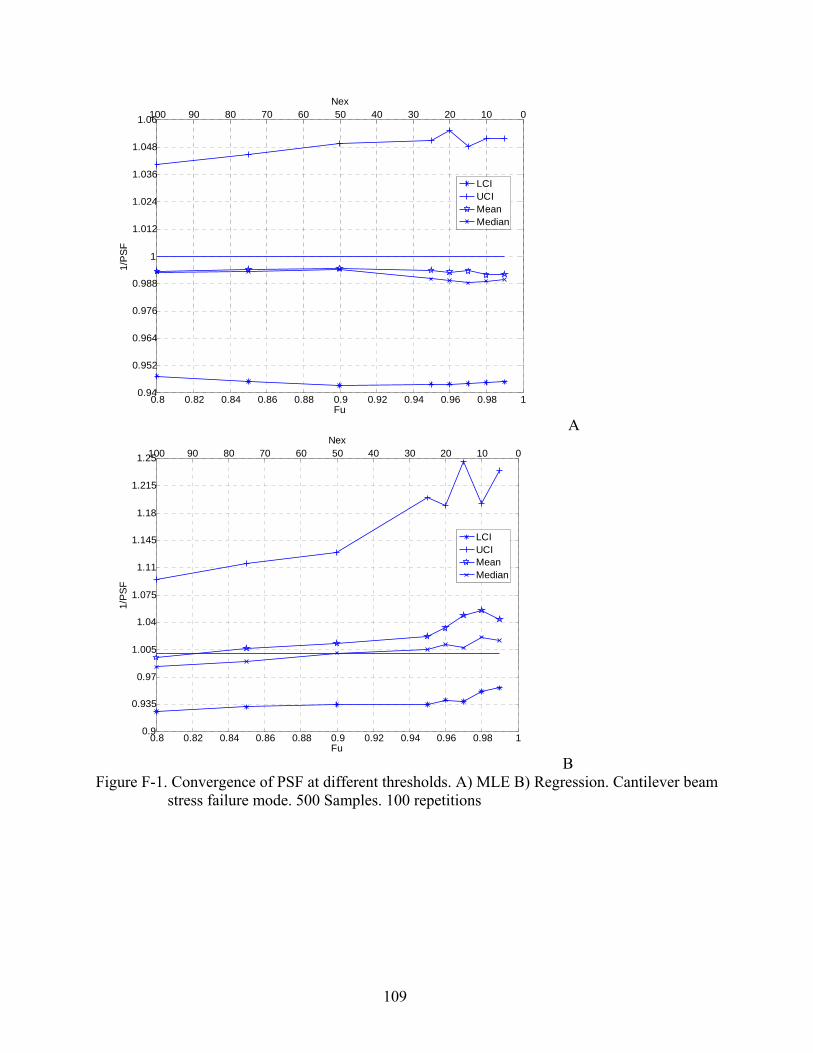
109

0.8 0.82 0.84 0.86 0.88 0.9 0.92 0.94 0.96 0.98 10.94

0.952

0.964

0.976

0.988

1

1.012

1.024

1.036

1.048

1.06

Fu

1/P

SF

LCIUCIMeanMedian

0102030405060708090100Nex

A

0.8 0.82 0.84 0.86 0.88 0.9 0.92 0.94 0.96 0.98 10.9

0.935

0.97

1.005

1.04

1.075

1.11

1.145

1.18

1.215

1.25

Fu

1/P

SF

LCIUCIMeanMedian

0102030405060708090100Nex

B Figure F-1. Convergence of PSF at different thresholds. A) MLE B) Regression. Cantilever beam

stress failure mode. 500 Samples. 100 repetitions

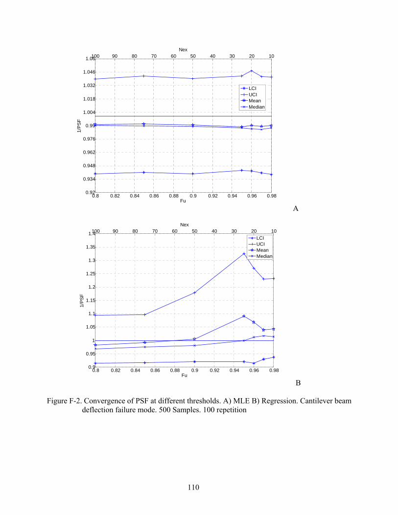
110

0.8 0.82 0.84 0.86 0.88 0.9 0.92 0.94 0.96 0.980.92

0.934

0.948

0.962

0.976

0.99

1.004

1.018

1.032

1.046

1.06

Fu

1/PS

F

LCIUCIMeanMedian

102030405060708090100Nex

A

0.8 0.82 0.84 0.86 0.88 0.9 0.92 0.94 0.96 0.980.9

0.95

1

1.05

1.1

1.15

1.2

1.25

1.3

1.35

1.4

Fu

1/PS

F

LCIUCIMeanMedian

102030405060708090100Nex

B

Figure F-2. Convergence of PSF at different thresholds. A) MLE B) Regression. Cantilever beam deflection failure mode. 500 Samples. 100 repetition

111

APPENDIX G STATISTICAL DISTRIBUTIONS ERROR PLOTS

Boxplot comparison of eind and eMTM at different reliability indices. ML=Maximum

Likelihood, Rg- Regression, QT – Quadratic fit to the Tail data between rS and ln( β ), LT –

Linear fit to the Tail data between rS and β , QH – Quadratic fit to half of the data between rS

and β .Dashed line inside the box depicts the mean and the solid line, the median. 1000

repetition

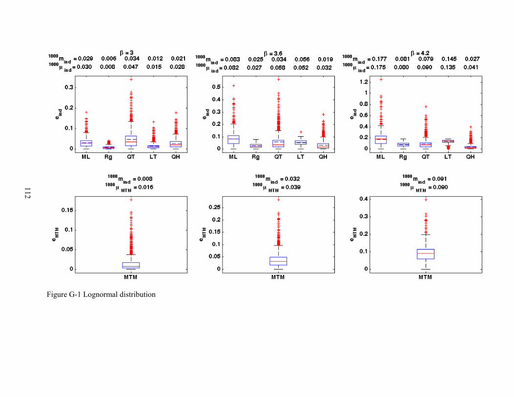
112

Figure G-1 Lognormal distribution

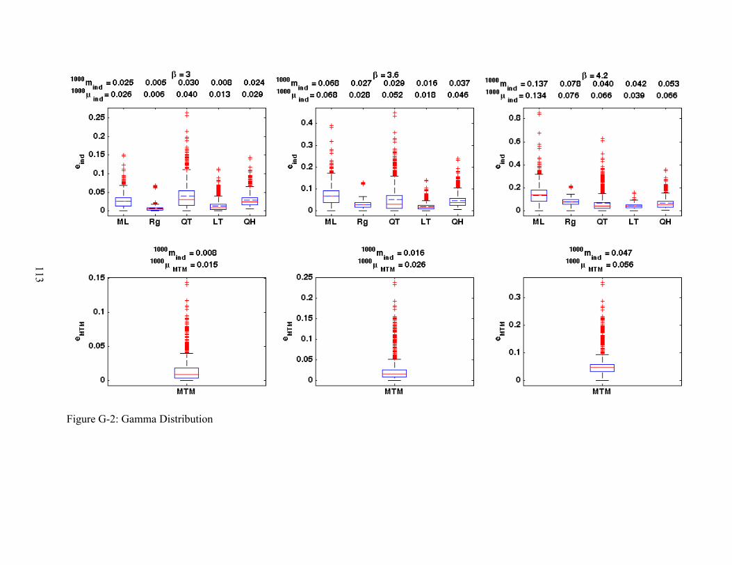
113

Figure G-2: Gamma Distribution

114

Figure G-3. Extreme Value type 1 Distribution

115

Figure G-4. Uniform Distribution.

116

Figure G-5. Rayleigh Distribution.

117

Figure G-6. Exponential Distribution.

118

Boxplot of η ratio. Different distributions

Figure G-7. Lognormal Distribution.

MTM

0.1

0.2

0.3

0.4

0.5

0.6

0.7

0.8

η

1000mη = 0.181

1000μη= 0.220

Figure G-8. Gamma Distribution.

MTM

0.1

0.2

0.3

0.4

0.5

0.6

0.7

0.8

η1000mη = 0.349

1000μη= 0.340

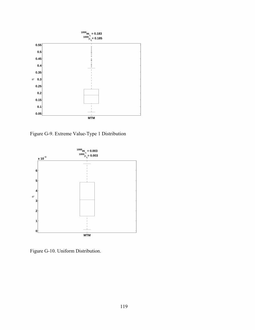
119

MTM0.05

0.1

0.15

0.2

0.25

0.3

0.35

0.4

0.45

0.5

0.55

η1000mη = 0.183

1000μη= 0.185

Figure G-9. Extreme Value-Type 1 Distribution

MTM0

1

2

3

4

5

6

x 10−3

η

1000mη = 0.003

1000μη= 0.003

Figure G-10. Uniform Distribution.

120

MTM0

0.2

0.4

0.6

0.8

1

η1000mη = 0.146

1000μη= 0.185

Figure G-11. Rayleigh Distribution.

MTM

0

0.1

0.2

0.3

0.4

0.5

0.6

0.7

η

1000mη = 0.241

1000μη= 0.276

Figure G-12. Exponential Distribution.

121

REFERENCES

Agarwal, H.; Lee, J.C.; Watson, L.T.; Renaud, J.E. 2004: A unilevel method for reliability based design optimization, Proceedings of the 45th AIAA/ASME/ASCE/AHS/ASC Structures, Structural Dynamics, and Material Conference, Palm Springs, CA, April 19-22, AIAA Paper 2004-2029. Agarwal H., Shawn E.G., Renaud J.E., Perez V.M., Watson. L.T. 2007: Homotopy Methods for Constraint Relaxation in Unilevel Reliability-based Design Optimization, Submitted to the ASME Journal of Mechanical Design Bassi, F.; Embrechts, P.; Kafetzaki, M. 1998: Risk Management and Quantile Estimation In: A Practical Guide to Heavy Tails, Edited by Adler, R. J., et al., Boston, Birkhaeuser, pp. 111-130 Beirlant, J.; Goegebeur, Y.; Segers, J.; Teugels, J. 2004: Statistics of Extremes: Theory and Applications, John Wiley & Sons Beirlant, J.; Vynckier, P.; Teugels, J.L. 1996: Excess Functions and Estimation of Extreme Value Index. Bernoulli, 2, pp:293-318 Boos, D.D. 1984: Using Extreme Value Theory to Estimate Large Percentiles, Technometrics, 26, pp:33-39 Caers, J.; Maes, M.A. 1998: Identifying Tails, Bounds and End-points of Random Variables. Structural Safety, Vol 20, pp 1-23 Castillo, E.; Hadi, A.S.; Balakrishnan, N.; Sarabia, J.M. 2005: Extreme Value and Related Models with Applications in Engineering and Science, Hoboken, New Jersey:Wiley Interscience Chen, S.; Nikolaidis, E.; Cudney, H. H. 1999: Comparison of Probabilistic and Fuzzy Set Methods for Designing under Uncertainty. Proceedings, AIAA/ASME/ASCE/AHS/ASC Structures, Structural dynamics, and Materials Conference and Exhibit, 2860-2874. Chiralaksanakul, A.; Mahadevan, S. 2005: Multidisciplinary Design Optimization Under Uncertainty, in press, Optimization and Engineering. Coles, S. 2001: An Introduction to Statistical Modeling of Extreme Values, London, England: Springer-Verlag Du, X.; Chen, W. 2004: Sequential Optimization and Reliability Assessment Method for Efficient Probabilistic Design,” Journal of Mechanical Design, Vol 126, No. 2, pp. 225 – 233. Du, X.; Sudjianto, A.; and Chen, W. 2004: An Integrated Framework for Optimization under Uncertainty Using Inverse Reliability Strategy, ASME Journal of Mechanical Design, Vol.126, No.4, pp. 561-764. Elishakoff, I. 2001: Interrelation between Safety Factors and Reliability, NASA report CR-2001-211309

122

Elishakoff, I. 2004: Safety Factors and Reliability: Friends or Foes? Kluwer Academic Publishers, Dordrecht, The Netherlands Frangopol, D.M. 1985: Structural Optimization Using Reliability Concepts. Journal of Structural Engineering. Vol. 111, no. 11, pp. 2288-2301 Frangopol, D. M.; Maute, K. 2003: Life-cycle Reliability-based Optimization of Civil and Aerospace Structures, Computers and Structures, Vol. 81, No. 7, pp. 397-410. Glasserman, P. 2004: Monte Carlo Methods in Financial Engineering. Springer Verlag Goel, T., Haftka, R.T., Shyy, W., Queipo, N.V.(2006) “Ensemble of Multiple Surrogates”, Structural and Multidisciplinary Optimization, 33(3) Gu, X.; Renaud, J.E.; Batill, S.M.; Brach, R.M.; Budhiraja, A.S. 2000: Worst Case Propagated Uncertainty of Multidisciplinary Systems in Robust Design Optimization. Structural and Multidisciplinary Optimization, 20(3), 190-213. Gurdal, Z.; Haftka, R.T.; Hajela, P. 1988: Design and Optimization of Laminated Composite Structures. New York: Wiley Hasofer, A.M. 1996: Parametric Estimation of Failure Probabilities. In: Mathematical Models for Structural Reliability Analysis. Edited by Casicati, F.; Roberts, B. Boca Raton, FL: CRC Press Hosking, J.R.M.; Wallis, J.R. 1987: Parameter and Quantile Estimation for the Generalized Pareto Distribution. Technometrics, Vol 29, no.3., pp. 339-349 Kharmanda. G and Olhoff N, 2007: Extension of Optimum Safety Factor Method to Nonlinear Reliability-based Design Optimization, Journal of Structural and Multidisciplinary Optimization, Vol. 34, No.5, pp. 367-380. Kharmanda. G., Olhoff N.,El-Hami .A. 2004: Optimum Values of Structural Safety Factors for a Predefined Reliability Level with Extension to Multiple Limit States, Journal of Structural and Multidisciplinary Optimization, Vol. 26, No.6, pp. 421-434. Kharmanda. G., Mohamed A., Lemaire M. 2002: Efficient Reliability-based Design Optimization Using Hybrid Space with Application to Finite Element Analysis, Journal of Structural and Multidisciplinary Optimization, Vol. 24, No.3, pp. 233-245. Kirjner-Neto, C.; Polak, E.; Kiureghian, A. D. 1998: An Outer Approximations Approach to Reliability-based Optimal Design of Structures, Journal of Optimization Theory and Applications, Vol. 98, No. 1, pp 1-16. Kiureghian, A. D.; Zhang, Y.; Li, C. C. 1994: Inverse Reliability Problem, Journal of Engineering Mechanics, Vol. 120, No. 5, pp. 1154-1159.

123

Kuschel, N.; and Rackwitz, R. 2000: A new approach for structural optimization of series systems, Applications of Statistics and Probability,Vol.2, No 8, pp987-994 Lee, J. O.; Yang, Y. S.; Ruy, W. S. 2002: A Comparative Study on Reliability-index and Target-performance-based Probabilistic Structural Design Optimization, Computers and Structures, Vol. 80, No. 3-4, pp. 257-269. Li, H.; Foschi, O. 1998: An Inverse Reliability Measure and Its Application, Structural Safety, Vol. 20, No. 3, pp. 257-270. Liu. D., Choi. K. K., Youn .B. D., Gorsich. D. 2006: Possibility-based Design Optimization Method for Design Problems with Both Statistical and Fuzzy Input Data, Journal of Mechanical Design, Vol 128, pp. 928-935. Liu. D., Choi. K. K., Youn .B. D. 2006: An Inverse Possibility Analysis Method for Possibility-Based Design Optimization, AIAA Journal, Vol 44, No. 11, pp. 2682-2689 Madsen, H. O.; Krenk, S.; Lind, N. C. 1986: Methods of Structural Safety, NJ: Prentice-Hall Maes, M.A.; Breitung, K. 1993: Reliability-Based Tail Estimation. Proceedings, IUTAM Symposium on Probabilistic Structural Mechanics (Advances in Structural Reliability Methods), San Antonio, Texas, 335-346 Maglaras, G.; Nikolaidis, E.; Haftka, R.T.; Cudney, H.H. 1997: Analytical-Experimental Comparison of Probabilistic methods and Fuzzy Set based Methods for Designing under Uncertainty, Structural Optimization, 13(2/3), pp. 69-80. Melchers, R. E. 1999: Structural Reliability Analysis and Prediction, New York: Wiley Metropolis, N. 1987: The Beginning of Monte Carlo Method, Los Alamos Science, Special Issue dedicated to Stanislaw Ulam: 125-130 Moore, G.E. 1965: Cramming More Components onto Integrated Circuits, Electronics, 38, (8). Mourelatos. Z.P., and Zhou, J. 2005: Reliability Estimation and Design with Insufficient Data Based on Possibility Theory, AIAA Journal, Vol 43, No. 8, pp 1696-1705 Myung J.I. 2003: Tutorial on Maximum Likelihood Estimation, Journal of Mathematical Psychology, 47, 90-100 Phadke M.S. 1989: Quality Engineering Using Robust Design, Englewood Cliffs, NJ: Prentice Hall Pickands, J. 1975: Statistical Inference Using Extreme Order Statistics. Annals of Statistics. Vol 3,119-131

124

Qu, X.; Haftka, R. T. 2004: Reliability-based Design Optimization Using Probabilistic Sufficiency Factor, Journal of Structural and Multidisciplinary Optimization, Vol. 27, No.5, pp. 314-325. Qu, X.; Haftka, R. T., Venkataraman, S., Johnson, T.F.2003: Deterministic and Reliability-Based Optimization of Composite Laminates for Cryogenic Environments, AIAA Journal, Vol 41, No.10, pp 2029-2036 Qu, X.; Singer, T.; Haftka, R. T. 2004:Reliability-based Global Optimization of Stiffened Panels Using Probabilistic Sufficiency Factor, Proceedings of the 45th AIAA/ASME/ASCE/AHS/ASC Structures, Structural Dynamics, and Material Conference, Palm Springs, CA, April 19-22,AIAA Paper 2004-1898. Qu,.X.,Venkataraman, S., Haftka, R T., Johnson, T.F. 2001: Reliability, Weight and Cost Tradeoffs in the Design of Composite Laminates for Cryogenic Environments, AIAA Paper 2001-1327, April 2001 Rackwitz, R.2000: Reliability Analysis – Past, Present and Future. 8th ASCE Speciality Conference on Probabilsitic Mechanics and Structural Reliability, 24-26 July, Notre Dame, IN, USA. Ramu, P.; Qu, X.; Youn, B.; Haftka, R.T.; Choi, K.K. 2006: Safety Factors and Inverse Reliability Measures, Int. J. Reliability and Safety, Vol. 1, Nos. 1/2 Rosenblatt, M. 1952: Remarks on a Multivariate Transformation, The Annals of Mathematical Statistics, 23(3), 470 – 472 Royset, J.O.; Kiureghian, A. D.; Polak, E. 2001: Reliability-based Optimal Structural Design by the Decoupling Approach,” Reliability Engineering and System Safety,Vol 73, No. 3, 2001, pp.213-221 Sakawa, M. 1993: Fuzzy sets and Interactive Multiobjective Optimization. Plenum press Smarslok, B. P.; Haftka, R. T.; Kim, N.H. 2006: Taking Advantage of Separable Limit States in Sampling Procedures. 47th AIAA/ASME/ASCE/AHS/ASC Structures, Structural Dynamics, and Materials Conference, AIAA 2006-1632, Newport, RI, May, Soundappan, P.; Nikolaidis, E.; Haftka, R.T.; Grandhi, R.; Canfield, R. 2004: Comparison of evidence theory and Bayesian Theory for Uncertainty Modeling, Reliability Engineering & System Safety, 85 (1-3): 295-311 Tu, J.; Choi, K. K.; Park, Y. H. 1999: A New Study on Reliability Based Design Optimization, Journal of Mechanical Design, ASME, Vol 121, No. 4, 557-564

125

Wu, Y T.; Shin Y.; Sues, R.; Cesare, M. 2001: Safety Factor Based Approach for Probability–based Design Optimization, Proceedings of 42nd AIAA/ ASME/ ASCE/AHS/ASC Structures, Structural Dynamics and Materials Conference, Seattle, WA, AIAA Paper 2001-1522. Youn B. D.; Choi K. K.; Du. L. 2005: Enriched Performance Measure Approach (PMA +) for Reliability-based Design Optimization,” AIAA Journal, Vol. 43, No. 4, pp. 874-884. Youn, B. D.; Choi, K. K.; Park, Y. H. 2003: Hybrid Analysis Method for Reliability-based Design Optimization, Journal of Mechanical Design, ASME, Vol. 125, No. 2, pp. 221-232.

126

BIOGRAPHICAL SKETCH

Palani Ramu was born in Chennai, India in 1978. He earned his BEng in Mechanical from

Madurai Kamaraj University, India in 1999. He worked at the Indian Institute of Technology,

Bombay and InfoTech - Pratt & Whitney Center of Excellence as Research Assistant and Design

Engineer respectively till 2002. In 2003, he started his graduate studies at the University of

Florida, Gainesville and worked towards a Ph.D in Aerospace Engineering. During his graduate

studies, he was a visiting researcher at the Leonardo Da Vinci University, Paris, France and was

awarded a summer fellowship at the Center for Space Nuclear Research – Idaho National Labs,

Idaho. His areas of interest include application of probability and statistical methods to design

aerospace structures, specifically highly reliable designs.

MULTIPLE TAIL MODELS INCLUDING INVERSE …plaza.ufl.edu/palramu/PalaniRamuDissertation.pdf · 1...

Documents

Transcript of MULTIPLE TAIL MODELS INCLUDING INVERSE …plaza.ufl.edu/palramu/PalaniRamuDissertation.pdf · 1...