Multiple Regression, Experimental Design and ANOVA · EMBnet Course – Introduction to Statistics...

EMBnet Course – Introduction to Statistics for Biologists 7 Mar 2007

Linear Models II

http://www.isrec.isb-sib.ch/~darlene/EMBnet/

Multiple Regression, Experimental Design and ANOVA

age

0.0 0.2 0.4 0.6 0.8 1.0

1015

20

0.0

0.2

0.4

0.6

0.8

1.0

sex

10 15 20 110 130 150 170

110

130

150

170

height


(Simple) Linear Regression (Review)Refers to drawing a (particular, special) line through a scatterplotUsed for 2 broad purposes:– Explanation– Prediction

Equation for a line to predict y knowing x (in slope-intercept form) looks like:

y = a + b*xa is called the intercept ; b is the slope


Regression PredictionThe regression prediction says:

when X goes up by 1 SD, predicted Y goes up **NOT by 1 SD**, but by only r SDs

This prediction can be expressed as a formula for a line in slope-intercept form:

predicted y = intercept + slope * x,

with slope = r * SD(Y)/SD(X)

intercept = mean(Y) – slope * mean(X)


Least Squares

Q: Where does this equation come from?

A: It is the line that is ‘best’ in the sense that it minimizes the sum of the squared errors in the vertical (Y) direction

*

*

*

*

*

errors

X

Y


Interpretation of parametersThe regression line has two parameters: the slope and the interceptThe regression slope is the average change in Y when X increases by 1 unitThe intercept is the predicted value for Y when X = 0If the slope = 0, then X does not help in predicting Y (linearly)


Multiple linear regressionYou can also use more than one ‘X ’ variable to predict Y : predicted y = a + b1x1 + b2x2Example : predict ventricular shortening velocity (Y) from blood glucose (X1) and age (X2)The ‘slopes’ b1 and b2 are called coefficientsThe prediction function for Y is still linear in the parameters (a, b1, b2)As in simple regression, minimize total squared deviation from the prediction surface (instead of a line it’s a plane or higher dim. hyperplane)


Example: cystic fibrosis> library(ISwR)

> data(cystfibr)

> round(cor(cystfibr),2)

age sex height weight bmp fev1 rv frc tlc pemax

age 1.00 -0.17 0.93 0.91 0.38 0.29 -0.55 -0.64 -0.47 0.61

sex -0.17 1.00 -0.17 -0.19 -0.14 -0.53 0.27 0.18 0.02 -0.29

height 0.93 -0.17 1.00 0.92 0.44 0.32 -0.57 -0.62 -0.46 0.60

weight 0.91 -0.19 0.92 1.00 0.67 0.45 -0.62 -0.62 -0.42 0.64

bmp 0.38 -0.14 0.44 0.67 1.00 0.55 -0.58 -0.43 -0.36 0.23

fev1 0.29 -0.53 0.32 0.45 0.55 1.00 -0.67 -0.67 -0.44 0.45

rv -0.55 0.27 -0.57 -0.62 -0.58 -0.67 1.00 0.91 0.59 -0.32

frc -0.64 0.18 -0.62 -0.62 -0.43 -0.67 0.91 1.00 0.70 -0.42

tlc -0.47 0.02 -0.46 -0.42 -0.36 -0.44 0.59 0.70 1.00 -0.18

pemax 0.61 -0.29 0.60 0.64 0.23 0.45 -0.32 -0.42 -0.18 1.00


Pairwise plots of cystic fibrosis vars> pairs(cystfibr)


R: multiple regression using lm> attach(cystfibr)> summary(lm(pemax~age+sex+height+weight))Call:lm(formula = pemax ~ age + sex + height + weight)Residuals:

Min 1Q Median 3Q Max -47.791 -18.683 2.747 13.413 43.190 Coefficients:

Estimate Std. Error t value Pr(>|t|)(Intercept) 70.66072 82.50906 0.856 0.402age 1.57395 3.13953 0.501 0.622sex -11.54392 11.23902 -1.027 0.317height -0.06308 0.80183 -0.079 0.938weight 0.79124 0.86147 0.918 0.369Residual standard error: 27.38 on 20 degrees of freedomMultiple R-Squared: 0.4413, Adjusted R-squared: 0.3296F-statistic: 3.949 on 4 and 20 DF, p-value: 0.01604


Model formulas in RA simple model formula in R looks something like: yvar ~ xvar1 + xvar2 + xvar3

We could write this model (algebraically) asY = a + b1*x1 + b2*x2 + b3*x3

By default, an intercept is included in the model - you don’t have to include a term in the model formulaIf you want to leave the intercept out:yvar ~ -1 + xvar1 + xvar2 + xvar3


Experimental Design – why do we care?Poor design costs:– time, money, ethical considerations

To ensure relevant data are collected, and can be analyzed to test the scientific hypothesis/ question of interest– Decide in advance how data will be analyzed– ‘Designing the experiment’ = ‘Planning the

analysis’The design is about the science (biology)


Variables (I)Statisticians call characteristics which can differ across individuals variablesTypes of variables– Categorical (also called qualitative)

• Examples: eye color, favorite television program

– Numerical (also called quantitative)• Examples: height, number of children,

fluorescence intensity


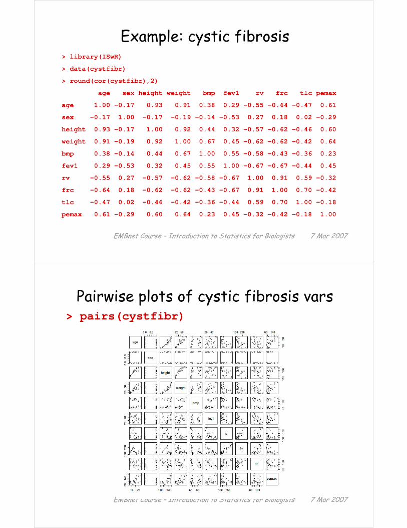
Variables (II)Categorical variables may be– Nominal – the categories have names, but no ordering

(e.g. eye color)

– Ordinal – categories have an ordering (e.g. `Always’, `Sometimes’, ‘Never’)

Numerical variables may be – Discrete – possible values can differ only by fixed

amounts (most commonly counting values)

– Continuous – can take on any value within a range (e.g. any positive value)


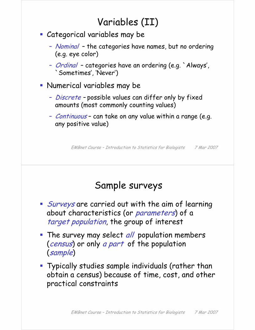
Sample surveys

Surveys are carried out with the aim of learning about characteristics (or parameters) of a target population, the group of interest

The survey may select all population members (census) or only a part of the population (sample)

Typically studies sample individuals (rather than obtain a census) because of time, cost, and other practical constraints


Random Variation

Also called ‘noise’How much do individuals in the sample differHere, ‘individuals’ could refer to:– animals– plants– people– plots of land– tissues


Sampling variability

Say we sample from a population in order to estimate the population mean of some (numerical) variable of interest (e.g. weight, height, number of children, etc.)We could use the sample mean as our guess for the unknown value of the population meanOur (observed) sample mean is very unlikely to be exactly equal to the (unknown) population mean just due to chance variation in samplingThus, it is useful to quantify the likely size of this chance variation (also called ‘chance error’ or ‘sampling error’, as distinct from ‘nonsampling errors’ such as bias)


The research process

Scientific question of interest

Decision on what data to collect (and how)

Collection and analysis of data

Conclusions, generalization

Communication and dissemination of results


Generic Question : Does a ‘treatment’ have an ‘effect’?

Examples :Does smoking cause cancer, heart disease, etc?

Does oat bran lower cholesterol?

Does echinacea prevent illness?

Does exercise slow the aging process?


Addressing the questionA basic means to address this type of question involves comparing two groups of study subjects – Control group: provides a baseline for

comparison

– Treatment group: group receiving the ‘treatment’


Experimental vs. Observational studiesControlled experiment : subjects assigned to groups by the investigator– randomization: protects against bias in assignment

to groups– blind, double-blind : protects against bias in

outcome assessment/measurement– placebo : fake ‘treatment’

Observational study : subjects ‘assign’ themselves to groups – confounder : associated with both group

membership and the outcome of interest


Observational studiesAdvantages– often easier to carry out – don’t ‘interfere’ with the system, what you see is

‘natural ’ rather than ‘artificial’– variation is biologically relevant, as it has been

unaltered– sometimes manipulation is not possible

Drawbacks– confounders– association (correlation) is NOT causation –

‘reverse’ causation


Confounding factors

Ideally, both the treatment and control groups are exactly alike in all respects (except for group membership)A confounding factor (or confounder) is associated with both the group membership and the responseCan you think of some examples ??


Replication, Randomization, Blocking

Replication – to reduce random variation of the test statistic, increases generalizabilityRandomization – to remove biasBlocking – to reduce unwanted variationIdea here is that units within a block are similar to each other, but different between blocks‘Block what you can, randomize what you cannot’


Focusing the study

Create a well-defined hypothesis– Does the question make sense?

Design a study that will test the hypothesisSatisfy sceptics


Three decisions

What measurements to make (response)

What conditions to study (treatments)

What experimental material to use (units)


Pilot StudyMaking sure the question makes sense in the system you will be studyingMaking sure the techniques work– practice – you don’t want to be learning the

technique in the real study!– identify problems and look for solutions– standardize techniques

Obtaining preliminary data– practice for statistical analyses– see if planned experiment size sufficient


A few commentsWith a well-planned and carried out controlled experiment, it is possible to infer causalityThis is not possible with observational studies due to the presence of confoundersWith confounding, it is not possible to tell whether the observed difference between groups is due to the treatment or to the confounder

Not always possible to carry out an experiment, due to practical and ethical reasons


Generic Question : Does a ‘treatment’ have an ‘effect’?

Does smoking cause cancer, heart disease, etc?Does oat bran lower cholesterol?Does echinacea prevent illness?Does exercise slow the aging process?Let’s think of how each of these might be examined experimentally and observationally (even if not practical) ...


Hibernation exampleGeneral question: How do changes in an animal’s environment cause the animal to start hibernating?What changes should be studied ??– temperature– photoperiod (day length)What measurement(s) to take?– nerve activity enzyme (Na+K+ATP-ase)What animal to study– golden hamster, 2 organs


Specific question

General question : How do changes in an animal’s environment cause the animal to start hibernating?=> Specific question : What is the effect of changing day length on the concentration of the sodium pump enzyme in two golden hamster organs?


Sources of variabilityVariability due to conditions of interest (wanted)– Day length (long vs. short)– Organ (heart vs. brains)

Variability in the response (NOT wanted): measurement error– Preparation of enzyme suspension– Instrument calibration

Variability in experimental units (NOT wanted)– Biological differences among hamsters– Environmental differences


Types of variability

Planned systematic (wanted)Chance variation (can handle this) Unplanned systematic (NOT wanted)– Can bias results– e.g. time of measurements


Hibernation questionsLong vs. short days : (How much) does day length affect enzyme concentrations?Hearts vs. brains : Different concentrations?Interaction : Is the difference in enzyme concentrations different for hearts and brains?Hamsters : How much variability between them?Measurement error : How big is the chance error of the enzyme concentration measurement process?


Basic designs: Completely randomizedFocus on 1 organ (heart, say)Random assignment: use chance to assign hamsters to long and short days‘Random’ is not the same as ‘haphazard’For balance, assign same number to short and longExample (8 hamsters):Long: 4, 1, 7, 2Short: 3, 8, 5, 6


Basic designs: Factorial crossingCompare 2 (or more) sets of conditions in the same experiment : Long vs. Short and Heart vs. BrainIn this example, there are 4 combinations of conditions: – Long/Heart, Long/Brain, Short/Heart,

Short/BrainExample (2 coin flips, say):

L/H: 7, 2 L/B: 4, 1S/H: 3, 5 S/B: 8, 6


Basic designs: Split plot/repeated measures

First, randomly assign Long days to 4 hamsters and Short days to the other 4Then, use each hamster twice : once to get Heart conc, and once to get Brain concThis design has units of different sizes for each factor– for day length, the unit is a hamster– for organ, the unit is a part of a hamster


SummaryOptimize precision of the estimates among main comparisons of interestMust satisfy scientific and physical constraints of the experimentYou can save a lot of time, money and heart-ache by consulting with an experienced analyst on design issues before any steps of the experiment have been carried out


(BREAK)


Brief review of hypothesis testing2 ‘competing theories’ regarding a population parameter:– NULL hypothesis H (‘straw man’)– ALTERNATIVE hypothesis A (‘claim’, or

theory you wish to test)H: NO DIFFERENCE – any observed deviation from what we expect

to see is due to chance variabilityA: THE DIFFERENCE IS REAL


Basic designs: Randomized blockSuppose that the hamsters came from 4 different litters, with 2 hamsters per litterExpect hamsters from the same litter to be more similar than hamsters from different littersCan take each pair of hamsters and randomly assign short or long to one member of each pairExample (coin flip, say):

S, L // L, S // S, L // S, L


Test statisticMeasure how far the observed data are from what is expected assuming the NULL H by computing the value of a test statistic (TS) from the dataThe particular TS computed depends on the parameter For example, to test the population mean μ, the TS is the sample mean (or standardized sample mean)


ExampleAn experiment is conducted to study the effect of exercise on the reduction of the cholesterol level in slightly obese patients considered to be at risk for heart attack. 80 patients are put on a specified exercise plan while maintaining a normal diet. At the end of 4 weeks the change in cholesterol level will be noted. It is thought that the program will reduce the average cholesterol reading by more than 25 points. Data:– sample mean = 27– sample SD = 18


Steps in hypothesis testing (I)1. Identify the population parameter being tested

Here, the parameter being tested is the population mean cholesterol reading μ

2. Formulate the NULL and ALT hypotheses

H: μ = 25 (or μ ≤ 25)A: μ > 25

3. Compute the TS

t = (27 – 25)/(18/√ 80) = .99


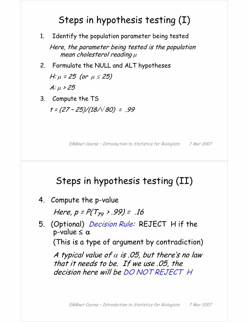
Steps in hypothesis testing (II)

4. Compute the p-valueHere, p = P(T79 > .99) = .16

5. (Optional) Decision Rule: REJECT H if thep-value ≤ α(This is a type of argument by contradiction)

A typical value of α is .05, but there’s no law that it needs to be. If we use .05, the decision here will be DO NOT REJECT H


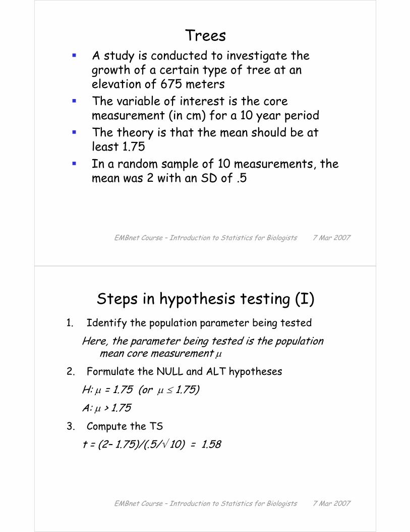
TreesA study is conducted to investigate the growth of a certain type of tree at an elevation of 675 metersThe variable of interest is the core measurement (in cm) for a 10 year periodThe theory is that the mean should be at least 1.75In a random sample of 10 measurements, the mean was 2 with an SD of .5


Steps in hypothesis testing (I)1. Identify the population parameter being tested

Here, the parameter being tested is the population mean core measurement μ

2. Formulate the NULL and ALT hypotheses

H: μ = 1.75 (or μ ≤ 1.75)A: μ > 1.75

3. Compute the TS

t = (2– 1.75)/(.5/√ 10) = 1.58


Steps in hypothesis testing (II)

4. Compute the p-valueHere, p = P(T9 > 1.58) = .07

5. (Optional) Decision Rule: REJECT H if thep-value ≤αIf we use α = .05, the decision here will beDO NOT REJECT H (but just barely!)


More treesNow say we are interested in whether the mean core measurement is the same in trees at 675 meters and trees at 825 meters

Now say we have a random sample also of size 10 of trees at 825 meters, with a mean core measurement of 2.65 cm and SD 1.15 cm

How might we test the null that the means are the same, against the alternative that they are different? ...


2-sample (z or t) test

(let’s think...)


Even more treesYou guessed it! Now say we are also interested in trees at 975 meters as well

Want to make a three-way comparison

Have a random sample (size 10 again) and find the mean is 2.5 and the SD is 1

How might we test the null that all three means are the same, against the alternative that they are different? (Pretend that we didn’t just make the two-way test ☺) ...


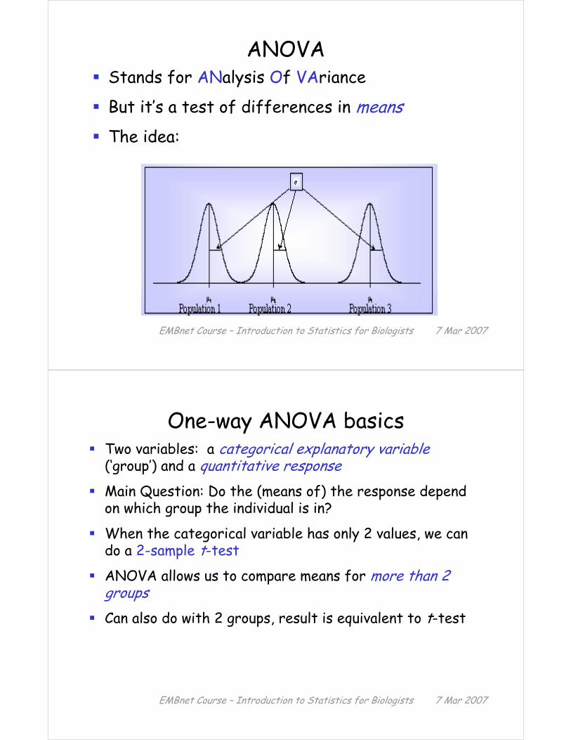
ANOVAStands for ANalysis Of VAriance

But it’s a test of differences in meansThe idea:


One-way ANOVA basicsTwo variables: a categorical explanatory variable(‘group’) and a quantitative responseMain Question: Do the (means of) the response depend on which group the individual is in?

When the categorical variable has only 2 values, we can do a 2-sample t-test

ANOVA allows us to compare means for more than 2 groupsCan also do with 2 groups, result is equivalent to t-test


The Observations yij

Treatment group

i = 1 i = 2 … i = k

means: m1 m2 … mk

yk, nk…y2, n2y1, n1

…………

yk,2…y22y12

yk,1…y21y11


How ANOVA worksANOVA measures two sources of variation in the data and compares their relative sizes

– Between group variation: for each data value look at the (squared) difference between its group mean mi and the overall mean m

– Within group variation: for each data value look at the (squared) difference between that value yij and its group mean mi


The ANOVA tableThe analysis is usually laid out in a table

For a one-way layout (where the response is assumed to vary according to grouping on one factor):

Σij(yij-m)2n-1Total

SSE/(n-k)Σij(yij-mi)2n-kError

*MST/MSESST/(k-1)Σi(mi-m)2k-1Treatment

p-valFMSSSdfSource

m = overall mean, mi = mean within group i


Assumptions

Have random samples from each separate population

The variance is the same in each treatment group

The samples are sufficiently large that the CLT holds for each sample mean (or the individual population distributions are normal)


EDA for ANOVA

Graphical investigation of group means– side-by-side box plots– multiple histograms

Check for normality– within group QQ plots

Within group summary statistics– group means, SDs

Assess variance ratio– usually done informally, could also do formal test

(R: var.test)


What does it mean when we reject H?

The null hypothesis H is a joint one: that all population means are equal

When we reject the null, that does NOT mean that the means are all different!

It means that at least one is different

To find out which is different, can do post hoctesting (pairwise t-tests, for example)


Additional aspectsWhy not start off doing separate (z or t) tests for each pair of samples? ...Testing the assumptions

Which mean(s) is/are not equal

– can do post hoc testing (pairwise t-tests, for example)

Multiple comparisons (multiple testing)

‘Data snooping’


Multiple ComparisonsIf the null is rejected, usually want to identify whichones are differentCan compare pairs of means using the 2-sample t-testNeed to adjust p-value threshold since we are doing multiple tests with the same data Several methods for doing this (e.g. Tukey)If a priori interested only in the difference between one pair of treatments, the study should be set up that way


Factorial crossingCompare 2 (or more) sets of conditions in the same experimentDesigns with factorial treatment structure allow you to measure interaction between two (or more) sets of conditions that influence the response – you will look at this in more detail during the exercises todayFactorial designs may be either observational or experimental


3 types of 2-factor factorial designs 2 experimental factors – you randomize treatments to each unit2 observational factors – you cross-classifyyour populations into groups and get a sample from each population1 experimental and 1 observational factor – you get a sample of units from each population, then use randomization to assign levels of the experimental factor (treatments), separately within each sample


InteractionInteraction is very common (and very important) in science Interaction is a difference of differencesInteraction is present if the effect of one factor is different for different levels of the other factorMain effects can be difficult to interpret in the presence of interaction, because the effect of one factor depends on the level of the other factor


Interaction plotno interaction interaction


More on model formulasWe can also include interaction terms in a model formula:

yvar ~ xvar1 + xvar2 + xvar3

Examples

– yvar ~ xvar1 + xvar2 + xvar3 + xvar1:xvar2

– yvar ~ (xvar1 + xvar2 + xvar3)^2

– yvar ~ (xvar1 * xvar2 * xvar3)


More on model formulasThe generic form is response ~ predictorsThe predictors can be numeric or factorOther symbols to create formulas with combinations of variables (e.g. interactions)

+ to add more variables- to leave out variables: to introduce interactions between two terms* to include both interactions and the terms

(a*b is the same as a+b+a:b)^n adds all terms including interactions up to order nI() treats what’s in () as a mathematical expression


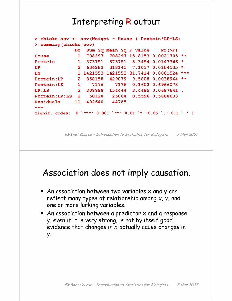
Interpreting R output

> chicks.aov <- aov(Weight ~ House + Protein*LP*LS)> summary(chicks.aov)

Df Sum Sq Mean Sq F value Pr(>F) House 1 708297 708297 15.8153 0.0021705 ** Protein 1 373751 373751 8.3454 0.0147366 * LP 2 636283 318141 7.1037 0.0104535 * LS 1 1421553 1421553 31.7414 0.0001524 ***Protein:LP 2 858158 429079 9.5808 0.0038964 ** Protein:LS 1 7176 7176 0.1602 0.6966078 LP:LS 2 308888 154444 3.4485 0.0687641 . Protein:LP:LS 2 50128 25064 0.5596 0.5868633 Residuals 11 492640 44785 ---Signif. codes: 0 `***' 0.001 `**' 0.01 `*' 0.05 `.' 0.1 ` ' 1


Association does not imply causation.

An association between two variables x and y can reflect many types of relationship among x, y, and one or more lurking variables.An association between a predictor x and a response y, even if it is very strong, is not by itself good evidence that changes in x actually cause changes in y.


Causal graphs

Dotted lines denote association. Solid lines denote causation. Solid lines are unidirectional (directed causal graph). Graphs are acyclic if no directed graph forms a loop (no variable can cause itself).

Z is a lurking variable in these schematics: a possibly unmeasured variable that may influence interpretation of the data

Reverse causation refers to erroneous conclusion that X causes Y when in fact Y causes X


Multiple Regression vs Causal Modeling

Multiple Regression

X1

X2

X3

X4

X5

Y

Q: How well do predictors predict (explain variances) in Y? What are independent effects when effects of other variables are controlled?

X1

X3 X4

X2 X5

Y

•• Causal ModelingCausal Modeling

Q: How well do predictorsrelate with regard to ultimateprediction of Y?


Multiple Regression

X1

X2

X3

X4

X5

Y

Y = a +β1X1 +β2X2 + β3X3 + β4X4 + β5X5 + e

•Y viewed as a linear function of combination of Xi

βi represent partial regression coefficients

•Only one Dependent Variable (Y)

•Hierarchical Regression: Subsets of predictors, added sequentially to identify the “best model” for the chosen dependent variable


Structure Modelsnn NonNon--significant predictors may not have significant predictors may not have ‘‘direct effectsdirect effects’’ on on DVDV

uuMay not be proximal causesMay not be proximal causes

uuMay be distal causes via May be distal causes via ‘‘indirect effectsindirect effects’’

n Causal modeling can be viewed as series of MR analyses Structural Structural

EquationsEquations::

XX33 = X= X11 + X+ X22

XX44 = X= X22 + X+ X33

XX55 = X= X22

Y = XY = X44 + X+ X55

X1

X3 X4

X2 X5

Y

Multiple Regression, Experimental Design and ANOVA · EMBnet Course – Introduction to Statistics...

Documents

Transcript of Multiple Regression, Experimental Design and ANOVA · EMBnet Course – Introduction to Statistics...