Noname manuscript No.(will be inserted by the editor)

Multiple Instance Learning via Gaussian Processes

Minyoung Kim and Fernando De la Torre

Received: date / Accepted: date

Abstract Multiple instance learning (MIL) is a binary classificationproblem withloosely supervised data where a class label is assigned onlyto a bag of instancesindicating presence/absence of positive instances. In this paper we introduce a novelMIL algorithm using Gaussian processes (GP). The bag labeling protocol of the MILcan be effectively modeled by the sigmoid likelihood through the max function overGP latent variables. As the non-continuous max function makes exact GP inferenceand learning infeasible, we propose two approximations: the soft-max approximationand the introduction of witness indicator variables. Compared to the state-of-the-artMIL approaches, especially those based on the Support Vector Machine (SVM), ourmodel enjoys two most crucial benefits: (i) the kernel parameters can be learned ina principled manner, thus avoiding grid search and being able to exploit a varietyof kernel families with complex forms, and (ii) the efficientgradient search for ker-nel parameter learning effectively leads to feature selection to extract most relevantfeatures while discarding noise. We demonstrate that our approaches attain superioror comparable performance to existing methods on several real-world MIL datasetsincluding large-scale content-based image retrieval problems.

Keywords Multiple Instance Learning· Gaussian Processes· Kernel Machines·Probabilistic Models

Minyoung KimDepartment of Electronics and IT Media Engineering,Seoul National University of Science & TechnologyTel.: +82-2-970-9020Fax: +82-2-970-7903E-mail: mikim21@gmail.com

Fernando De la TorreThe Robotics Institute,Carnegie Mellon University, Pittsburgh, PA 15213, USATel.: +1-412-268-4706Fax: +1-412-268-5571E-mail: ftorre@cs.cmu.edu

2

1 Introduction

The paper deals with the multiple instance problem, a very important topic in ma-chine learning and data mining. We begin with its formal definition. In the standardsupervised classification setup, we have training data{(xi ,yi)}ni=1 which are labeledat the instance level. In the binary classification setting,yi ∈ {+1,−1}. In multipleinstance learning (MIL) (Dietterich et al, 1997) problem, on the other hand, the as-sumption is rather loosen in the following manner: (i) one isgivenB bags of instances{Xb}Bb=1 where each bag,Xb = {xb,1, . . . ,xb,nb}, consists ofnb instances (∑bnb = n),and (ii) the labels are provided only at the bag-level in a waythat for each bagb,Yb = −1 if yi = −1 for all i ∈ Ib, andYb = +1 if yi = +1 for some i∈ Ib, whereIbindicates the index set for instances in bagb.

The MIL is considered to be more realistic than standard classification setup dueto its notion of bag in conjunction with the bag labeling protocol. Two most typi-cal applications are image retrieval (Zhang et al, 2002; Gehler and Chapelle, 2007)and text classification (Andrews et al, 2003). For instance,the content-based imageretrieval fits well the MIL framework as an image can be seen asa bag comprisedof smaller regions/patches (i.e., instances). Given a query for a particular object, onemay be interested in deciding only whether the image contains the queried object(Yb = +1) or not (Yb =−1), instead of solving the more involved (and probably lessrelevant) problem of labeling every single patch in the image. In text classification,one is more concerned with the concept/topic (i.e., bag label) of an entire paragraphthan labeling each of the sentences that comprise the paragraph. The MIL frameworkis also directly compatible with other application tasks including the object detec-tion (Viola et al, 2005) and the identification of proteins (Tao et al, 2004).

Although we only consider the original MIL problem defined asabove, thereare other alternative problems and generalization. For instance, themultiple instanceregressiondeals with the real-valued outputs instead of binary labels(Dooly et al,2002; Ray and Page, 2001), and themultiple instance clusteringtackles the multipleinstance problems in unsupervised situations (Zhang and Zhou, 2009; Zhang et al,2011). The MIL problem can be extended to more generalized forms. One typicalgeneralization is to modify the bag positive condition to bedetermined by somecol-lection of positive instances, instead of a single one (Scott et al, 2003). Essentiallyand more generally, one can obtain other types of generalized MIL problems by spec-ifying how the collection of underlying instance-level concepts is combined to formthe label of the bag (Weidmann et al, 2003).

Traditionally, the MIL problem was tackled by specially tailored algorithms; forexample, the hypothesis class of axis-parallel rectanglesin the feature space has beenintroduced in (Dietterich et al, 1997), which is iteratively estimated to contain in-stances from positive bags. In (Maron and Lozano-Perez, 1998), the so-called di-verse density (DD) is defined to measure proximity between a bag and a positiveintersection point. Another line of research considers theMIL problem as a standardclassification problem at a bag-level via proper development of kernels or distancemeasures on the bag space (Wang and Zucker, 2000; Gartner etal, 2002; Tao et al,2004; Chen et al, 2006). Particularly it subsumes the set kernels for SVMs (Gartner

3

et al, 2002; Tao et al, 2004; Chen et al, 2006) and the Hausdorff set distances (Wangand Zucker, 2000).

A different perspective that regards the MIL as a missing-label problem was re-cently emerged. Unlike the negative instances which are alllabeled negatively, thelabels of instances in the positive bags are considered as latent variables. The latentlabels have additional positive bag constraints, namely that at least one of them ispositive, or equivalently,∑i

yi+12 ≥ 1 for i ∈ Ib such thatYb = +1. In this treatment,

a fairly straightforward approach would be to formulate a standard (instance-level)classification problem (e.g., SVM) that can be optimized over the model and thelatent variables simultaneously. Themi-SVMapproach of (Andrews et al, 2003) isderived in this manner.

More specifically, the following optimization problem is solved for both the hy-perplane parameter vectorw and the output variables{yi}:

min{yi},w,{ξi}

12||w||2 +C

n

∑i=1

ξi

s.t. ξi ≥ 1−yiw>xi, ξi ≥ 0 for all i,

yi =−1 for all i ∈ Ib s.t. Yb =−1.

∑i∈Ib

yi +12≥ 1 for all b s.t.Yb = +1. (1)

Although the latent instance label treatments are mathematically appealing, adrawback of such approaches is that they involve a (mixed) integer programmingwhich is generally difficult to solve. There have been several heuristics or approxi-mate solutions such as those proposed in (Andrews et al, 2003). Recently, the deter-ministic annealing (DA) algorithm has been employed (Gehler and Chapelle, 2007),which approximates the original problem to a continuous optimization by introducingbinary random variables in conjunction with the temperature-scaled (convex) entropyterm. The DA algorithm begins with a high temperature to solve a relatively easyconvex-like problem, and iteratively reduces the temperature with the warm starts(initialized at the solution obtained from the previous iteration).

Instead of dealing with all instances in a positive bag individually, a more in-sightful strategy is to focus on themost positiveinstance, often referred to as thewitness, which is responsible for determining the label of a positive bag. In the SVMformulation, theMI-SVMof (Andrews et al, 2003) directly aims at maximizing themargin of the instance with the most positive confidence w.r.t. the current modelw(i.e., maxi∈Ib〈w,xb,i〉). An alternative formulation has been introduced in theMICAalgorithm (Mangasarian and Wild, 2008), where they indirectly form a witness us-ing convex combination over all instances in a positive bag.TheEM-DD algorithmof (Zhang et al, 2002) extends the diverse density frameworkof (Maron and Lozano-Perez, 1998) by incorporating the witnesses. In (Gehler andChapelle, 2007) the DAalgorithms have also been applied to the witness-identifying SVMs, exhibiting supe-rior prediction performance to existing approaches.

Even though some of these MIL algorithms, especially the SVM-based discrim-inative methods, are quite effective for a variety of situations, most approaches are

4

non-probabilistic, thus unable to capture the underlying generative process of the MILdata formation. In this paper1 we introduce a novel MIL algorithm using the Gaus-sian process (GP), which we callGPMIL. Motivated from the fact that a bag label issolely determined by the instance that has the highest confidence toward the positiveclass, we design the bag class likelihood as the sigmoid function over the maximumGP latent variables on the instances. By marginalizing out the latent variables, wehave a nonparametric, nonlinear probabilistic modelP(Yb|Xb) that fully respects thebag labeling protocol of the MIL.

Dealing with a probabilistic bag class model is not completely new. For instance,the Noisy-OR model suggested by (Viola et al, 2005) represents a bag label prob-ability distribution, where the learning is formulated within the functional gradi-ent boosting framework (Friedman, 1999). A similar Noisy-OR modeling has re-cently been proposed with Bayesian treatment by (Raykar et al, 2008). In their ap-proaches, however, the bag class model is built from theinstance-levelclassifica-tion modelsP(yi |xi), more specifically,P(Yb = −1|Xb) = ∏i∈Ib P(yi = −1|xi) andP(Yb = +1|Xb) = 1−P(Yb = −1|Xb), which may incur several drawbacks. First ofall, it involves additional modeling effort for the instance-level classifiers, which maybe unnecessary, or only indirectly relevant to the bag classdecision. Moreover, theNoisy-OR model combines the instance-level classifiers in aproduct form, treatingeach instance independently. This ignores the impact of potential interaction amongthe neighboring instances, which may be crucial for the accurate bag class predic-tion. On the other hand, our GPMIL represents the bag class model directly with-out employing probably unnecessary instance-level classifiers. The interaction amongthe instances is also incorporated through the GP prior thatessentially enforces thesmoothness regularization along the neighboring structure of the instances.

In addition to the above-mentioned advantages, the most important benefit of theGPMIL, especially contrasted with the SVM-based approaches, is that the kernel hy-perparameters can be learned in a principled manner (e.g., empirical Bayes), thusavoiding grid search and being able to exploit a variety of kernel families with com-plex forms. Another promising aspect is that the efficient gradient search for kernelparameter learning effectively leads to feature selectionto extract most relevant fea-tures while discarding noise. One caveat of the GPMIL is thatit is intractable toperform exact GP inference and learning due to the non-continuous max function.We remedy it by proposing two approximation strategies: thesoft-max approxima-tion and the use of witness indicator variables which can be further optimized bythe deterministic annealing schedule. Both approaches often exhibit more accurateprediction than most recent SVM variants.

The paper is organized as follows. After briefly reviewing the Gaussian processand introducing notations used throughout the paper in Sec.2, our GPMIL frameworkis introduced in Sec. 3 with the soft-max approximation for inference and learning.The witness variable based approximation for GPMIL is described in Sec. 4, while we

1 It is an extension of our earlier work (conference paper) published in (Kim and De la Torre, 2010). Weextend the previous work broadly in two aspects: i) More technical details and complete derivations areprovided for Gaussian process and our approaches based on it, which makes the manuscript comprehensiveand self-contained, and ii) The experimental evaluation includes more extensive multiple instance learningdatasets including the SIVAL image retrieval database and the drug activity datasets.

5

also suggest the deterministic annealing optimization. After discussing relationshipwith existing MIL approaches in Sec. 5, the experimental results of the proposedmethods on both synthetic data and real-world MIL benchmarkdatasets are providedin Sec. 6. We conclude the paper in Sec. 7.

2 Review on Gaussian Processes

In this section we briefly review the Gaussian process model.The Gaussian processis a nonparametric, nonlinear Bayesian regression model. For the expositional con-venience, we first consider alinear regression from inputx ∈ R

d to output f ∈ R:

f = w>x+ ε, where w ∈ Rd is the model parameter andε ∼N (0,η2). (2)

Given n i.i.d. data points{(xi, fi)}ni=1, where we often use vector notations,f =[ f1, . . . , fn]> andX = [x1, . . . ,xn]

>, we can express the likelihood as:

P(f|X,w) =n

∏i=1

P( fi |xi ,w) = N (f;Xw,η2I). (3)

We then turn this into a Bayesian nonparametric model by placing prior onw andmarginalizing it out. With a Gaussian priorP(w) = N (0, I), it is easy to see that

P(f|X) =∫

P(f|X,w)P(w)dw = N (f;0,XX>+ η2I) N (f;0,XX>). (4)

Here, we letη → 0 to have a noise-free model. Although we restrict ourselvesto thetraining data, adding a new test pair(x∗, f∗) immediately leads to the following jointGaussian by concatenating the test point with the training data, namely

P(

[f∗f

]|[

x∗X

]) = N

([f∗f

];

[00

],

[x>∗ x∗ x>∗ X>

Xx∗ XX>

]). (5)

From (5), the predictive distribution forf∗ is analytically available as a conditionalGaussian:

P( f∗|x∗, f,X) = N ( f∗;x>∗ X>(XX>)−1f,x>∗ x∗−x>∗ X>(XX>)−1Xx∗). (6)

A nonlinear extension of (4) is straightforward by replacing the finite dimensionalvectorw by an infinite dimensional nonlinear functionf (·) 2. TheGaussian process(GP) is a particular choice of prior distribution on functions, which is characterizedby thecovariance function(i.e., the kernel function)k(·, ·) defined on the input space.Formally, a GP withk(·, ·) satisfies:

Cov( f (xi), f (x j )) = k(xi ,x j), for anyxi andx j . (7)

2 We abuse the notationf to indicate either a function or a response variable evaluated atx (i.e., f (x)interchangeably.

6

In fact, any distribution onf that satisfies (7) is a GP. Forf that follows the GP priorwith k(·, ·), marginalizing outf produces a nonlinear version of (4),

P(f|X) = N (f;0,K β ), (8)

whereK β is the kernel matrix on the input dataX (i.e.,[K β ]i, j = kβ (i, j)). Here,β inthe subscript indicates the (hyper)parameters of the kernel function (e.g., for the RBFkernel,β includes the length scale, the magnitude, and so on). As the dependencyon β is clear, we will sometimes drop the subscript for notational convenience. For anew test inputx∗, by lettingk(x∗) = [k(x1,x∗), . . . ,k(xn,x∗)]>, we have a predictivedistribution for a test responsef∗, similar to (6). That is,

P( f∗|x∗, f,X) = N ( f∗;k(x∗)>K−1f,k(x∗,x∗)−k(x∗)>K−1k(x∗)). (9)

When the GP is applied for regression or classification problems, we often treatf aslatentrandom variables indexed by the training data samples, and introduce theactual (observable) output variablesy = [y1, . . . ,yn]

> which are linked tof through alikelihood modelP(y|f)= ∏n

i=1P(yi | fi). In the Appendix, we review in greater detailstwo most popular likelihood models that yield GP regressionand GP classification.

3 Gaussian Process Multiple Instance Learning (GPMIL)

In this section we introduce a novel Gaussian process (GP) model for the MIL prob-lem, which we denote byGPMIL. Our approach builds a bag class likelihood modelfrom the GP latent variables, where the likelihood is the sigmoid of themaximumlatent variables.

Note that the bagb is comprised ofnb points Xb = {xb,1, . . . ,xb,nb}. Accord-ingly, we assign the GP latent variables to the instances in the bagb, and we denotethem byFb = { fb,1, . . . , fb,nb}. One can regardfi (∈ Fb) as aconfidencescore to-ward the (instance-level) positive class forxi (∈ Xb). That is, the sign offi indicatesthe (instance-level) class labelyi , and its magnitude implies how confident it is. Inthe MIL, our goal is to devise a bag class likelihood modelP(Yb|Fb) instead of theinstance-level modelP(yi | fi). Note that the latter is a special case of the former sincean instance can be seen as a singleton bag. Once we have the bagclass likelihoodmodel, we can then marginalize out all the latent variablesF = {Fb}Bb=1 under theBayesian formalism using the GP priorP(F|X) given the entire inputX = {Xb}Bb=1.

Now, consider the situation where the bagb is labeled as positive (Yb = +1). Thechance is determined solely by the single point that is themost likely positive(i.e., thelargestf ). The larger the confidencef , the higher the chance is. The other instancesdo not contribute to the bag label prediction no matter what their confidence scoresare3. Hence, we can let:

P(Yb = +1|Fb) ∝ exp(maxi∈Ib

fi). (10)

3 We provide a better insight about our argument here. It is true that any other instances can make abag positive, but it is the instance with the highest confidence score (what we calledmost likely positiveinstance) that solely determines the bag label. In other words, to have an effect on the label of a bag, aninstance needs to get the largest confidence score. In formalprobability terms, the instancei can determinethe bag label only for the events that assign the highest confidence toi. It is also important to note that eventhough maxi∈B fi indicates a single instance, max function examinesall instances in the bag to find it.

7

Similarly, the odds of the bagb being labeled as negative (Yb =−1) is affected solelyby the single point which is theleast likely negative. As far as that point has a negativeconfidencef , the label of the bag is negative, and the larger the confidence− f , thehigher the chance is. This leads to the model:

P(Yb =−1|Fb) ∝ exp(mini∈Ib− fi). (11)

Combining (10) and (11), we have the following bag class likelihood model:

P(Yb|Fb) =1

1+exp(−Ybmaxi∈Ib fi). (12)

Note also that (12), in the limiting case where all the bags become singletons (i.e.,classical supervised classification), is equivalent to thestandard Gaussian processclassification model with the sigmoid link4.

When incorporating the likelihood model (12) into the GP framework, one bot-tleneck is that we have non-differentiable formulas due to the max function. We ap-proximate it by the soft-max5: max(z1, . . . ,zm)≈ log∑i exp(zi). This leads to the ap-proximated bag class likelihood model:

P(Yb|Fb) ≈1

1+exp(−Yb log∑i∈Ib efi )

=1

1+(∑i∈Ib efi )−Yb. (13)

Whereas the soft-max is often good approximation to the max function, it shouldbe noted that unlike the standard GP classification with the sigmoid link, the neg-ative log-likelihood− logP(Yb|Fb) = log(1+ (∑i∈Ib efi )−Yb) is not a convex func-tion of Fb for Yb = +1 (although it is convex forYb = −1). This corresponds to anon-convex optimization in the approximated GP posterior computation and learningwhen the Laplace or variational approximation methods are adopted. However, usingthe (scaled) conjugate gradient search with different starting iterates, one can properlyobtain a well-approximated posterior with a meaningful setof hyperparameters.

Before we proceed further to the details of inference and learning, we briefly dis-cuss the benefits of the GPMIL compared to the existing MIL methods. As mentionedearlier, the GPMIL directly models the bag class distribution, without suboptimallyintroducing instance-level models such as the Noisy-OR model of (Viola et al, 2005).Also, framed in the GP framework, the posterior estimation and the hyperparame-ter learning can be accomplished by simple gradient search with similar complexityas the standard GP classification, while it enables probabilistic interpretation (e.g.,uncertainty in prediction). Moreover, we have a principledway to learn the kernelhyperparameters under the Bayesian formalism, which is notproperly handled byother kernel-based MIL methods.

4 So, it is also possible to have a probit version of (12), namely P(Yb|fb) = Φ(Ybmaxi∈Ib fi ), whereΦ(·)is the cumulative normal function.

5 It is well known that the soft-max provides relatively tightbounds for the max, maxmi=1 zi ≤

log∑mi=1 exp(zi)≤maxmi=1 zi + logm. Another nice property is that the soft-max is a convex function.

8

f*,n *f*,1 f*,2

x*,n *x*,2x*,1

*Y

...

...

F* =

* =X

fb,n bfb,1

bY

fb,2

xb,n bxb,2xb,1

...

...

Fb =

b =X

1Y

1F

1X

bY

bF

bX

*Y

*F

*X

BY

BF

BX......

......

... ...

||| |||

Test DataTrain Data

Fig. 1 Graphical model for GPMIL.

3.1 Posterior, Evidence, and Prediction

From the latent-to-output likelihood model (13), our generative GPMIL model canbe depicted in a graphical representation as Fig. 1. Following the GP framework, allthe latent variablesF = {F1, . . . ,FB}= { fb,i}b,i are dependent on one another as wellas on all the training input pointsX = {X1, . . . ,XB} = {xb,i}b,i , conforming to thefollowing distribution:

P(F|X) = N (F;0,K), (14)

Similarly, for a new test bagX∗ = {x∗,1, . . . ,x∗,n∗} together with the correspondinglatent variablesF∗ = { f∗,1, . . . , f∗,n∗}, we have a joint Gaussian prior on the concate-nated latent variables,{F∗,F}, from which the predictive distribution onF∗ can be

9

derived as (by conditional Gaussian):

P(F∗|X∗,F,X) = N

(F∗; k(X∗)>K−1F, k(X∗,X∗)−k(X∗)>K−1k(X∗)

), (15)

wherek(X∗) is the(n×n∗) train-test kernel matrix whosei j -th element isk(xi ,x∗, j),andk(X∗,X∗) is the(n∗×n∗) test-test kernel matrix whosei j -th element isk(x∗,i ,x∗, j).

Under the usual i.i.d. assumption, the entire likelihoodP(Y = [Y1, . . . ,YB]|F) isthe product of the individual bag likelihoodsP(Yb|Fb) in (13). That is,

P(Y|F) =B

∏b=1

P(Yb|Fb)≈B

∏b=1

11+(∑i∈Ib efi )−Yb

. (16)

Equipped with (14) and (16), one can compute the posterior distributionP(F|Y,X) ∝P(F|X)P(Y|F) and the evidence (or the data likelihood)P(Y|X) =

∫F P(F|X)P(Y|F),

where the GP learning maximizes the evidence w.r.t. the kernel hyperparameters (alsoknown as the empirical Bayes). However, similar to the GP classification cases, thenon-Gaussian likelihood term (16) causes intractability in the exact computation, andwe resort to some approximation. Here we focus on the Laplaceapproximation6

where its application to standard GP classification is very popular and reviewed inAppendix.

The Laplace approximation essentially replaces the product P(Y|F)P(F|X) by aGaussian with the mean equal to the mode of the product, and the covariance equal tothe inverse Hessian of the product evaluated at the mode. Forthis purpose, we rewrite

P(Y|F)P(F|X) = exp(−S(F)) · |K |−1/2 · (2π)−n/2,

where S(F) =B

∑b=1

l(Yb,Fb)+12

F>K−1F,

l(Yb,Fb) =− logP(Yb|Fb)≈ log(

1+(∑i∈Ib

efi )−Yb

). (17)

We first find the minimum ofS(F), namely

F = argminF

S(F), (18)

where the optimum is denoted byF. Solving (18) can be done by gradient searchas usual. Unlike the standard GP classification, however, notice thatS(F) is a non-convex function ofF since the Hessian ofS(F), H + K−1, is generally not positivedefinite, whereH is the block diagonal matrix whoseb-th block has thei j -th entry

[Hb]i j = ∂ 2l(Yb,Fb)∂ fi∂ f j

for i, j ∈ Ib. Although this may hinder obtaining the global mini-

mum easily,S(F) is bounded below by 0 (from (17)), and the (scaled) conjugateor

6 Although it is feasible, here we do not take the variational approximation into consideration for sim-plicity. Unlike the standard GP classification, it is difficult to perform, for instance, the Expectation Prop-agation (EP) approximation since the moment matching, the core step in EP that minimizes the KL diver-gence between the marginal posteriors, requires the integration over the likelihood function in (13), whichrequires further elaboration.

10

Newton-type gradient search with different initial iterates can yield a reliable solu-tion.

We then approximateS(F) by a quadratic function using its Hessian evaluated atF, namelyH(F)+K−1. Yet, in order to enforce a convex quadratic form, we need toaddress the case thatH +K−1 is not positive definite, which although very rare, couldhappen as gradient search only discovers a point close (not exactly the same) to localminima. We approximate it to the closest positive definite matrix by projecting it ontothe PSD cone. More specifically, we letQ ≈ H +K−1, with Q = ∑i max(λi ,ε)viv>i ,whereλ andv are the eigenvalues/vectors ofH +K−1, andε is a small positive con-stant. In this wayQ is a positive definite matrix closest to the Hessian with precisionε. Letting Q beQ evaluated atF, we approximateS(F) by the following quadraticfunction (i.e., using the Taylor expansion)

S(F)≈ S(F)+12(F− F)>Q(F− F), (19)

which leads to Gaussian approximation forP(F|Y,X)

P(F|Y,X)≈N (F; F,Q−1). (20)

The data likelihood (i.e., evidence) immediately follows from the similar approx-imation,

P(Y|X,θ )≈ exp(−S(F))|Q|−1/2|K |−1/2. (21)

We then maximize (21) (so-calledevidence maximizationorempirical Bayes) w.r.t. thekernel parametersθ by gradient search.

More specifically, the negative log-likelihood,NLL = − logP(Y|X,θ ), can beapproximately written as:

NLL =B

∑b=1

l(Yb, Fb)+12

F>K−1F+12

log|I +KH |. (22)

The gradient of the negative log-likelihood with respect toa (scalar) kernel parameterθm (i.e.,θ = {θm}) can then be derived easily as follows:

∂NLL∂θm

=−12

α>( ∂K

∂θm

)α +

12

tr

((H−1 +K)−1

( ∂K∂θm

))+

12

tr

((H +K−1)−1

( ∂H∂θm

)),

(23)

where

α = K−1F and( ∂H

∂θm

)

i, j= tr

((∂H i, j

∂F

)>(I +KH )−1

( ∂K∂θm

)α

). (24)

Here,tr(A) is the trace of the matrixA. In the implementation, one can exploit the

fact that∂H i, j

∂F is highly sparse (only the corresponding block ofFb can be non-zero).The overall learning algorithm is depicted in Algorithm 1.Given a new test bagX∗ = {x∗,1, . . . ,x∗,n∗}, it is easy to derive the predictive

distribution for the corresponding latent variablesF∗ = { f∗,1, . . . , f∗,n∗}. Using the

11

Algorithm 1 GPMIL LearningInput: Initial guessθ , the tolerance parameterτ .Output: Learned hyperparametersθ .(a) FindF from (18) for currentθ .(b) ComputeQ using the PSD cone projection.(c) Maximize (21) w.r.t.θ .if ||θ −θold||> τ then

Go to (a).else

Returnθ .end if

Gaussian approximated posterior (20) together with the conditional Gaussian prior(15), we have:

P(F∗|X∗,Y,X) =∫

P(F∗|X∗,F,X)P(F|Y,X)dF

≈∫

P(F∗|X∗,F,X)N (F; F,Q−1)dF

= N

(F∗; k(X∗)>K−1F, k(X∗,X∗)+k(X∗)>(K−1Q−1K−1−K−1)k(X∗)

).

(25)

Finally, the predictive distribution for the test bag classlabelY∗ can be obtained bymarginalizing outF∗, namely

P(Y∗|X∗,Y,X) =

∫P(F∗|X∗,Y,X)P(Y∗|F∗)dF∗. (26)

The integration in (26) generally needs further approximation. If one is only inter-ested in the mean prediction (i.e., the predicted class label), it is possible to approx-imate P(F∗|X∗,Y,X) by a delta function at its mean (mode),µ := k(X∗)>K−1F,which yields the test prediction:

Class(Y∗)≈ sign

(1

1+(∑i∈∗eµi )−1 −0.5

). (27)

4 GPMIL using Witness Variables

Although the approach in Sec. 3 is reasonable, one drawback is that the target func-tion we approximate (i.e.,S(F)) is not in general a convex function (due to the non-convexity of− logP(Yb|Fb)), where we perform the PSD projection step to find theclosest convex function in the Laplace approximation. In this section, we address thisissue in a different way by introducing the so-calledwitness latent variableswhichindicate the most probably positive instances in the bags.

For each bagb, we introduce the witness indicator random variablesPb = [pb,1, . . . , pb,nb]>,

wherepb,i represents the probability thatxb,i is considered as awitnessof the bagb.We call an instance awitnessif it contributes to the likelihoodP(Yb|Fb). Note that∑i pb,i = 1, andpb,i ≥ 0 for all i ∈ Ib. In the MIL, asP(Yb|Fb) is solely dependent on

12

the most likely positive instance, it is ideal to put all the probability mass to a singleinstance as:

pb,i =

{1 if i = argmaxj fb, j

0 otherwise(28)

Alternatively, it is also possible to define a soft witness assignment7 using a sigmoidfunction:

pb,i =exp(λ fb,i)

∑ j∈Ib exp(λ fb, j), (29)

whereλ is the parameter that controls the smoothness of the assignment.OncePb is given, we then define the likelihood as a sigmoid of the weighted sum

of fi ’s with weightspi ’s:

P(Yb|Fb,Pb) =1

1+exp(−Yb ∑i pb,i fb,i). (30)

The aim here is to replace themaxor thesoft-maxfunction in the original derivationby theexpectation, ∑i pb,i fb,i , a linear function ofFb given the witness assignmentPb. Notice that givenPb, the negative log-likelihood of (30) is a convex function ofFb.

In the full Bayesian treatment, one marginalizes outPb, namely

P(Yb|Fb) =∫

P(Yb|Fb,Pb)P(Pb|Fb)dPb, (31)

whereP(Pb|Fb) is a Dirac’s delta function with the point support given as (28) or(29). However, this simply leads to the very non-convexity raised by the originalversion of our GPMIL. Rather we pursue the coordinate-wise convex optimizationby separating the process of approximatingP(Yb|Fb) into two individual steps: (i)find the witness indicatorPb from Fb using (28) or (29), and (ii) (while fixingPb)represent the likelihood as the sigmoid of the weighted sum (30), and perform poste-rior approximation. We alternate these two steps until convergence. Note that in thissetting the Laplace approximation becomes quite similar tothat of the standard GPclassification, having the additional alternating optimization as an inner loop.

4.1 (Optional) Deterministic Annealing

When we adopt the soft witness assignment in the above formulation, it is easy to seethat (29) is very similar to the probability assignment in the deterministic annealing(i.e., Eq. (11) of (Gehler and Chapelle, 2007)) while the smoothness parameterλnow acts as the inverse temperature in the annealing schedule. Motivated by this, wecan have a annealed version of posterior approximation. More specifically, it initiallybegins with a smallλ (large temperature) corresponding to a uniform-likePb, andrepeats the followings: perform a posterior approximationstarting from the optimumFb in the previous stage to get a newFb, then increaseλ to reduce the entropy ofPb.

7 This has a close relation to (Gehler and Chapelle, 2007)’s deterministic annealing approach to SVM.Similar to (Gehler and Chapelle, 2007), one can also consider a scheduled annealing, where the inverse ofthe smoothness parameterλ in (29) serves as the annealing temperature. See Sec. 4.1 forfurther details.

13

5 Related Work

This section briefly reviews/summarizes some typical approaches to MIL problemsthat are related to our models.

The pioneering work by (Dietterich et al, 1997) introduces the multiple instanceproblem, where they suggest a specific type of hypothesis class that can be learnediteratively to meet the positive bag/instance constraints. Since this work, there havebeen considerable research results on MIL problems. Most ofthe existing approachescan roughly belong to one of two different techniques: 1) directly learning a dis-tance/similarity metric between bags, and 2) learning a predictor model while prop-erly dealing with missing labels.

The former category includes: the diverse density (DD) of (Maron and Lozano-Perez, 1998) that aims to estimate proximity between a bag and a positive intersectionpoint, the EM-DD of (Zhang et al, 2002) that extends the DD by introducing wit-ness variables, and several kernel/distance measures proposed by (Wang and Zucker,2000; Gartner et al, 2002; Tao et al, 2004; Chen et al, 2006).In the other category, themost popular and sophisticated SVM framework has been exploited to find reason-able predictors. Themi-SVM(Andrews et al, 2003) is derived by formulating SVM-like optimization with the MIL’s bag constraints. The difficult integer programminghas been mitigated by the technique of deterministic annealing (Gehler and Chapelle,2007).

Apart from instance-level predictors, the idea of focusingon themost positiveinstance or thewitness, has been studied considerably. In the SVM framework,MI-SVMof (Andrews et al, 2003) directly maximizes the margin of theinstance with themost positive confidence. Alternatively, theMICA algorithm (Mangasarian and Wild,2008) parameterized witnesses as linear weighted sums overall instances in positivebags. Our GPMIL model can also be seen as a witness-based approach as the bagclass likelihood is dominated by the maximally confident instance either via sigmoidsoft-max modeling or via introducing witness random variables.

Some of the recent multiple instance algorithms have close relationships withthe witness technique similar to ours. We briefly discuss twointeresting approaches.In (Li et al, 2009), the CBIR problem is particularly considered where the regionsof interest can be seen as witnesses or key instances in positive bags. They formed aconvex optimization problem iteratively by finding violated key instances and com-bining them via multiple kernel learning. The optimizationinvolves a series of stan-dard SVM subproblems, and can be solved efficiently by a cutting plane algorithm.In (Liu et al, 2012), the key instance detection problem is tackled/formulated withina graph-based voting framework, which is formed either by a random walk or aniterative rejection algorithm.

We finally list some of more recent MIL algorithms. In (Anticand Ommer, 2012),a MIL problem is tackled by two alternating tasks of learningregular classifiers andimputing missing labels. They introduced the so-calledsuperbags, a random ensem-ble of sets of bags, aimed for decoupling two tasks to avoid overfitting and improverobustness. Instead of building bag-level distance measures, (Wang et al, 2011) pro-poses a new approach of forming aclass-to-bagdistance metric. The goal is to reflect

14

the semantic similarities between class labels and bags. The maximum margin opti-mization is formulated and solved by parameterizing the distance metrics.

Apart from typical treatments that consider bags having a finite number of in-stances, the approach in (Babenko et al, 2011) regards bags as low dimensional man-ifolds embedded in high dimensional feature space. The geometric manifold struc-ture of the manifold bags is then learned from data. This can be essentially seenas employing a particular bag kernel that preserves the geometric constraints thatreside in data. In (Fu et al, 2011), they focus on the problem of efficient instanceselection under large instance spaces. An adaptive instance selection algorithm is in-troduced, which alternates between instance selection andclassifier learning in aniterative manner. In particular, the instance selection isseeded by a simple kerneldensity estimator on negative instances.

There are several unique benefits of having the GP framework in MIL problems.First, by using GP, choosing parameters of the kernel/modelcan be done in a princi-pled manner (e.g., empirical Bayes of maximizing data likelihood) unlike some ad-hoc methods by SVM. Also, the parameters in GP models are random variables, andhence can be marginalized out within the Bayesian probabilistic framework to yieldmore flexible models. Furthermore, apart from other non-parametric kernel machines,one can interpret the underlying kernels more directly as the covariance functions,for which certain domain knowledge can be effectively exploited. In our MIL for-mulation, the bag label scoring model process is specifically treated as a covariancefunction over the input instance space. More importantly, we have observed empiri-cally that the proposed GPMIL approaches achieve often times much more accurateprediction than existing methods including recent SVM-based MIL algorithms.

6 Experiments

In this section we conduct experimental evaluation for bothartificially generated dataand several real-world benchmark datasets. The latter includes the MUSK datasets (Di-etterich et al, 1997), image annotation, and text classification datasets traditionallywell-framed in multiple instance learning setup. Furthermore, we test the proposedalgorithms on the large-scale content-based image retrieval task using the SIVALdataset (Rahmani and Goldman, 2006).

We run two different approximation schemes for our GPMIL, which are denotedby: (a)GP-SMX = the soft-max approximation with the PSD projection described inSec. 3, and (b)GP-WDA = the approximation using the witness indicator variableswith the deterministic annealing optimization discussed in Sec. 4. In theGP-SMX, theGP inference/learning optimization is done by the (scaled)conjugate gradient searchwith different starting iterates. In theGP-WDA, we start from a large temperature (e.g.,λ = 1e−1), and decrease it in log-scale (e.g.,λ ← 10·λ ) until there is no significantchange in the quantities to be estimated. For both methods, we first estimate kernelhyperparameters by empirical Bayes (i.e., maximizing the evidence likelihood), thenuse the learned hyperparameters to the test prediction. TheGPMIL is implementedin Matlab based on the publicly available GP codes from (Rasmussen and Williams,2006).

15

−30 −20 −10 0 10 20 30−2.5

−2

−1.5

−1

−0.5

0

0.5

1

1.5

2

2.5

input (x)

outp

ut (

f and

y)

f(x)y(x)

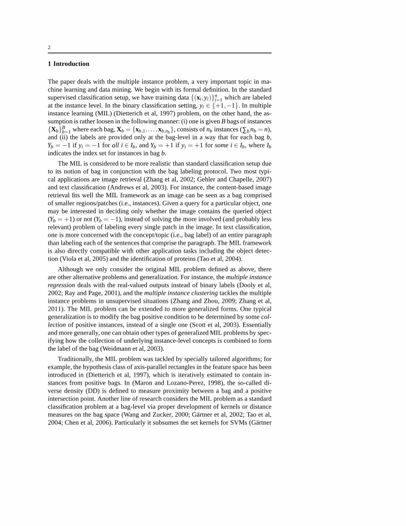
Fig. 2 Visualization of the synthetic 1D dataset. It depicts the instance-level input and output samples,where the bag formation is done by randomly grouping the instances. See text for details.

In the following section, we first demonstrate the performance of the proposedalgorithms on artificially generated data.

6.1 Synthetic Data

In this synthetic setup, we test the capability of the GPMIL on estimating the kernelhyperparameters accurately from data. We construct the synthetic 1D dataset gener-ated by a GP prior with random formation of the bags. The first step is to samplethe input data pointsx uniformly from the real line[−30,30]. For the 1000 sam-ples generated, the latent variablesf are randomly generated from the GP prior dis-tribution with the covariance matrix set equal to the(1000× 1000) kernel matrixfrom the input samples. The kernel has a particular form, specifically the RBF kernelk(x,x′) = exp(−||x− x′||2/2σ2), where the hyperparameter is set toσ = 3.0. TheRBF kernel form is assumed known to the algorithms, and the goal is to estimateσas accurately as possible. Given the sampledf , the actual instance-level class out-put y is then determined by:y = sign( f ). Fig. 2 depicts the instance-level input andoutput samples (i.e.,f (andy) vs.x).

To form the bags, we perform the following procedure. For each bagb, we ran-domly assign the bag labelYb uniformly from{+1,−1}. The number of instancesnb

is also chosen uniformly at random from{1, . . . ,10}. WhenYb = −1, we randomlyselectnb instances from the negative instances of the 1000-sample pool. On the otherhand, whenYb = +1, we flip the 10-side fair coin to decide the positive instanceportion pp∈ {0.1,0.2, . . . ,1.0}, with which the bag is constructed fromdpp× nbeinstances selected randomly from the positive instances and the rest (also randomly)from the negative instance pool. We generate 100 bags. We repeat the above proce-dure randomly 20 times.

We then perform the GPMIL hyperparameter learning startingfrom the initialguessσ = 1.0. We compute the averageσ estimated for 20 trials. The results are:3.2038±0.2700 for the GP-SMX approach, and3.0513±0.2149 for the GP-WDA,

16

which are very close to the true valueσ = 3.0. This experimental result highlightsunique benefit of our GPMIL algorithms, namely that we can estimate the kernel pa-rameters precisely in a principled manner, which is difficult to be achieved by otherexisting MIL approaches that rely on heuristic grid search on the hyperparameterspace.

6.2 Competing Approaches

In this section we perform extensive comparison study of ourGPMIL approachesagainst the state-of-the-art MIL algorithms. The competing algorithms are summa-rized below. The datasets, evaluation setups, and prediction results are provided inthe following sections.

– GP-SMX: The proposed GPMIL algorithm that implements the soft-maxapprox-imation with the PSD projection.

– GP-WDA: The proposed GPMIL algorithm that incorporates the witness indica-tor random variables optimized by deterministic annealing.

– mi-SVM: The instance-level SVM formulation by treating the labelsof instancesin positive bags as missing variables to be optimized (Andrews et al, 2003).

– MI-SVM : The bag-level SVM formulation that aims to maximize the margin ofthe most positive instance (i.e., witness) with respect to the current model (An-drews et al, 2003).

– AL-SVM : The deterministic annealing extension of the instance-level mi-SVMby introducing binary random variables that indicate the positivity/negativity ofthe instances (Gehler and Chapelle, 2007).

– ALP-SVM : Further extension ofAL-SVM by incorporating extra constraints onthe expected number of positive instances per bag (Gehler and Chapelle, 2007).

– AW-SVM : The deterministic annealing extension of the witness-basedMI-SVMapproach (Gehler and Chapelle, 2007).

– EMDD: Probabilistic approach to find witnesses of the positive bags to estimatediverse densities (Zhang et al, 2002). We use Jun Yang’s implementation, referredto asMultiple Instance Learning Library8.

– MICA : SVM formulation that indirectly represents the witnessesusing convexcombination over instances in positive bags (Mangasarian and Wild, 2008). Thelinear program formulation for the MICA has been implemented in MATLAB.

Unless stated otherwise, all the kernel machines includingour GPMIL algorithmsemploy the RBF kernel. For the SVM-based methods, the scale parameter of the RBFkernel is chosen as the median of the pairwise pattern distances. The hyperparametersare optimized using cross validation. Other parameters areselected randomly.

8 Available at http://www.cs.cmu.edu/∼juny/MILL.

17

6.3 Standard Benchmark Datasets

6.3.1 The MUSK Datasets

The MUSK datasets (Dietterich et al, 1997) have served widely as the benchmarkdataset for demonstrating performance of MIL algorithms. The datasets consist ofthe description of molecules using multiple low-energy conformations. The featurevectorx is of 166-dimensional. There are two different types of bag formation de-noted by MUSK1 and MUSK2, where the MUSK1 has approximatelynb = 6 con-formations (instances) per bag, while the MUSK2 takesnb = 60 instances per bag onaverage.

For comparison with the existing MIL algorithms, we follow the experimentalsetting similar to that of (Andrews et al, 2003; Gehler and Chapelle, 2007), wherewe conduct 10-fold cross validation. This is further repeated 5 times with different(random) partitions, and the average accuracies are reported. The test accuracies areshown in Table 1.

Our GPMIL algorithms, for both approximation strategiesWDA andSOFT-MAX,exhibit superior classification performance to the existing approaches for the twoMUSK datasets. One exception is the MICA where their reported error is the smalleston the MUSK2 dataset. This can be mainly due to the use of L1-regularizer in theMICA that yields a sparse solution suitable for the large-scale MUSK2 dataset. As isalso alluded in (Gehler and Chapelle, 2007), it may not be directly comparable withthe other methods.

6.3.2 Image Annotation

We test the algorithms on the image annotation datasets devised by (Andrews et al,2003) from the COREL image database. Each image is treated asa bag comprisedof the segments (instances) that are represented as featurevectors of color, text, andshape descriptors. Three datasets are formed for the objectcategories, tiger, elephant,and fox, regarding images containing the object as positive, and the rest as negative.

We follow the same setting as the original paper: There are 100/100 positive/negativebags, each of which contains 2∼ 13 instances. Similar to (Andrews et al, 2003;Gehler and Chapelle, 2007), we conduct 10-fold cross validation. This is further re-peated 5 times with different (random) partitions. Table 1 shows the test accuracies.The proposed GPMIL algorithms achieve significantly higheraccuracy than the bestcompeting approaches most of the time. Comparing two approximation methods forGPMIL, GP-WDA often outperformsGP-SMX, implying that the approximation basedon witness variables followed by a proper deterministic annealing schedule can bemore effective than the soft-max approximation with the spectral convexification.

6.3.3 Text Classification

We next demonstrate the effectiveness of the GPMIL algorithm on the text categoriza-tion task. We use the MIL datasets provided by (Andrews et al,2003) obtained from

18

Table 1 Test accuracies (%) on MUSK and Image Annotation Datasets. We report the accuracies of theproposed GPMIL algorithms,GP-SMX (soft-max approximation) andGP-WDA (witness variables with de-terministic annealing). In AW-SVM and AL-SVM, for the two annealing schedules suggested by (Gehlerand Chapelle, 2007), we only show the ones with smaller errors. Boldfaced numbers indicate the bestresults.

Dataset GP-SMX GP-WDA mi-SVM MI-SVM AL-SVM ALP-SVM AW-SVM EMDD MICAMUSK1 88.5± 3.5 89.5± 3.4 87.6± 3.5 79.3± 3.7 85.7± 3.0 86.5± 3.4 85.7± 3.1 84.6± 4.2 84.0± 4.4MUSK2 87.9± 3.8 87.2± 3.7 83.8± 4.8 84.2± 4.5 86.3± 4.0 86.1± 4.7 83.4± 4.2 84.7± 3.2 90.3± 5.8TIGER 87.1± 3.6 87.4± 3.6 78.7± 5.0 83.3± 3.3 78.5± 4.8 85.2± 3.2 82.7± 3.5 72.1± 4.0 81.3± 3.1

ELEPHANT 82.9± 4.0 83.8± 3.8 82.7± 3.6 81.5± 3.5 79.7± 2.1 82.8± 3.0 81.9± 3.4 77.5± 3.4 81.7± 4.7FOX 63.2± 4.1 65.7± 4.9 58.7± 5.7 57.9± 5.5 63.7± 5.4 65.7± 4.3 63.3± 4.2 52.2± 5.9 58.3± 6.2

Table 2 Test accuracies (%) on text classification. Boldfaced numbers indicate the best results.

Dataset GP-WDA mi-SVM MI-SVM EMDDTST1 94.4 93.6 93.9 85.8TST2 85.3 78.2 84.5 84.0TST3 86.1 87.0 82.2 69.0TST4 85.3 82.8 82.4 80.5TST7 80.3 81.3 78.0 75.4TST9 70.8 67.5 60.2 65.5TST10 80.4 79.6 79.5 78.5

the well-known TREC9 database. The original data are composed of 54000 MED-LINE documents annotated with 4903 subject terms, each defining a binary concept.Each document (bag) is decomposed into passages (instances) of overlapping win-dows of 50 or less words. Similar to the settings in (Andrews et al, 2003), a smallersubset is used, where the data are publicly available9. The dataset is comprised of 7concepts (binary classification problems), each of which has roughly the same num-ber (about 1600) of positive/negative instances from 200/200 positive/negative bags.

In Table 2 we report the average test accuracies of the GPMIL with theWDA ap-proach, together with those of competing models from (Andrews et al, 2003). ForMI-SVM and mi-SVM, only the linear SVM results are shown since the linear ker-nel outperforms polynomial/RBF kernels most of the time. Inthe GPMIL we alsoemploy the linear kernel. We see that for a large portion of the problem sets, ourGPMIL exhibits significant improvement over the methods provided in the originalpaper (EM-DD, mi-SVM, and MI-SVM).

6.4 Localized Content-Based Image Retrieval

The task of content-based image retrieval (CBIR) is perfectly fit to the MIL formu-lation. A typical setup of the CBIR problem is as follows: oneis given a collectionof training images where each image is labeled as+1 (−1) indicating existence (ab-sence) of a particular concept or object in the image. Treating an entire image as a

9 http://www.cs.columbia.edu/∼andrews/mil/datasets.html.

19

bag, and the regions/patches in the image as instances, it exactly reduces to the MILproblem: we only have bag-level labels where at least one positive region implies thatthe image is positive.

For this task, we use the SIVAL (Spatially Independent, Variable Area, and Light-ing) dataset (Rahmani and Goldman, 2006). The SIVAL datasetis composed of 1500images of 25 different object categories (60 images per category). The images ofsingle objects are photographed with highly diverse backgrounds, while the spatiallocations of the objects within images are arbitrary. This image acquisition setup canbe more realistic and challenging than the popular COREL image database in whichobjects are mostly centered in the images occupying majorities of images.

The instance/bag formation is as follows: Each image is transformed into theYCbCr color space followed by pre-processing using a wavelet texture filter. Thisgives rise to six features (three colors and three texture features) per pixel. Then theimage is segmented by the IHS segmentation algorithm (Zhangand Fritts, 2005).Each segment (instance) of the image is represented by the 30-dim feature vector bytaking averages of color/texture features over pixels in the segment itself as well asthose from its four neighbor segments (N, E, S, W). It ends up with 31 or 32 instancesper bag.

We then form binary MIL problems via one-vs-all strategy (i.e., considering eachof 25 categories as the positive class and the other categories as negative): For eachcategoryc, we take 20 random (positive) images fromc, and randomly select oneimage from each of the classes other thanc (that is, collecting 24 negative images).These 44 images serve as the training set, and all the rest of the images are used fortesting. This procedure is repeated randomly for 5 times, and we report the averageperformance (with standard errors) in Table 3.

Since the label distributions of the test data are highly unbalanced (for each cat-egory, the negative examples take about 97% of the test bags), we used the AUROC(Area-Under ROC) measure instead of the standard error rates. In this result, we ex-cluded MICA not only because its performance is worse than best performing onesfor most categories, but also it often takes a large amount oftime to converge to op-timal solutions. As shown in the results, the proposed GPMILmodels perform bestmost of the problem sets, exhibiting superb or comparable performance to the existingmethods. The Gaussian process priors used in our models haveeffects of smoothingby interpolating the latent score variables across unseen test points, which is shownto be highly useful for improving generalization performance.

20Table 3 Test accuracies (AUROC scores) on the SIVAL CBIR dataset. Boldfaced numbers indicate the best results within the marginof significance.

Category GP-SMX GP-WDA mi-SVM MI-SVM AL-SVM ALP-SVM AW-SVM EMDD

AjaxOrange 90.05± 8.61 94.20± 8.48 75.47± 5.20 63.57± 7.60 87.68± 3.53 83.72± 5.97 86.28± 12.66 56.83± 11.22

Apple 61.69± 2.69 67.43± 3.11 54.70± 4.24 47.20± 3.99 50.77± 4.93 52.45± 2.24 61.26± 6.54 54.63± 2.79

Banana 67.69± 7.05 68.92± 4.51 61.79± 5.72 55.82± 3.45 60.52± 4.62 62.05± 4.63 63.89± 4.87 59.86± 5.18

BlueScrunge 72.04± 6.46 68.13± 1.21 65.04± 7.66 67.17± 9.40 71.94± 5.20 67.65± 5.01 71.82± 7.60 66.04± 3.03

CandleWithHolder 89.49± 3.35 86.58± 7.54 80.85± 2.12 76.73± 4.47 76.81± 5.57 77.67± 5.34 84.70± 2.15 69.36± 5.86

CardboardBox 76.35± 15.89 73.53± 3.81 65.03± 4.03 64.93± 5.32 68.86± 4.26 67.31± 4.72 68.04± 3.33 58.42± 1.12

CheckeredScarf 94.85± 5.36 92.29± 8.52 81.44± 1.28 80.01± 2.27 88.04± 2.06 90.93± 2.93 88.63± 1.31 89.90± 2.37

CokeCan 96.55± 3.14 95.14± 3.30 93.61± 0.86 79.07± 6.74 92.49± 2.94 88.39± 4.32 92.45± 1.16 72.59± 5.20

DataMiningBook 77.07± 11.68 72.82± 5.40 69.82± 9.63 58.13± 2.84 75.25± 6.02 72.95± 6.19 78.86± 6.35 71.75± 7.26

DirtyRunningShoe 79.16± 3.18 82.39± 4.88 74.90± 4.83 67.73± 2.66 77.71± 1.93 81.00± 3.34 82.17± 4.01 80.14± 3.89DirtyWorkGloves 61.32± 4.91 80.96± 3.65 73.86± 3.80 63.07± 4.67 76.77± 4.84 66.59± 3.14 76.96± 6.08 66.11± 3.12

FabricSoftnerBox 96.13± 6.50 94.94± 3.29 95.53± 0.72 83.17± 6.23 96.17± 2.04 93.20± 3.84 97.52± 2.01 75.65± 12.77

FeltFlowerRug 92.98± 8.71 87.80± 7.47 85.91± 2.12 84.52± 1.40 89.40± 1.89 89.39± 3.78 90.75± 3.31 76.42± 7.66

GlazedWoodPot 63.66± 8.42 67.40± 2.68 50.93± 4.34 47.73± 6.49 55.75± 4.40 57.41± 3.58 58.47± 5.69 73.45± 6.68GoldMedal 82.82± 4.20 71.59± 5.19 83.40± 11.63 52.07± 8.25 86.89± 2.79 86.18± 4.75 87.68± 4.06 74.38± 6.90

GreenTeaBox 93.73± 2.79 93.56± 5.00 88.50± 6.93 86.64± 7.17 95.47± 2.75 92.67± 1.00 93.48± 1.55 79.92± 7.70

JuliesPot 87.23± 9.08 91.78± 11.23 82.12± 17.26 51.87± 3.29 84.37± 10.52 80.86± 10.58 88.88± 6.76 83.06± 8.39

LargeSpoon 60.01± 4.74 63.30± 3.46 54.16± 3.73 57.02± 3.18 54.38± 1.53 55.08± 1.81 54.13± 0.76 59.01± 1.49

RapBook 67.43± 3.33 67.73± 6.60 60.33± 3.14 57.18± 2.93 60.80± 4.60 60.59± 1.82 59.31± 3.78 55.78± 3.25

SmileyFaceDoll 80.65± 2.28 75.32± 5.76 75.52± 1.73 74.46± 5.98 81.05± 4.54 68.55± 4.72 81.47± 9.52 65.47± 6.77

SpriteCan 80.31± 9.91 79.84± 7.29 72.75± 3.21 75.38± 7.28 74.07± 5.91 75.99± 7.66 78.57± 7.47 64.36± 5.03

StripedNotebook 89.29± 3.40 90.45± 5.40 70.64± 7.34 63.26± 3.31 88.10± 2.86 81.08± 4.33 88.90± 2.66 61.47± 4.25

TranslucentBowl 79.71± 5.79 72.62± 3.75 79.33± 8.82 62.48± 3.02 78.96± 5.32 74.72± 4.48 77.12± 6.58 75.08± 6.90

WD40Can 90.41± 5.78 79.82± 4.42 88.99± 3.30 83.02± 2.66 92.02± 1.83 88.34± 3.05 94.10± 1.17 70.57± 6.23

WoodRollingPin 71.17± 6.73 75.26± 4.47 54.72± 1.62 61.72± 4.06 57.09± 2.28 59.09± 3.80 64.57± 2.91 58.90± 3.81

21

6.5 Drug Activity Prediction

Next we consider the drug activity prediction task with the publicly available artificialmolecule dataset10. In the dataset, the artificial molecules were generated such thateach feature value represents the distance from the molecular surface when alignedwith the binding sites of the artificial receptor. A moleculebag is then comprised ofall likely low-energy configurations or shapes for the molecule. More details on thedata synthesis can be found in (Dooly et al, 2002).

The data generation process is quite similar to the MUSK datasets, while a notableaspect is that the real-valued labels are introduced. The label for a molecule is the ratioof the binding energy to the maximum possible binding energygiven the artificialreceptor, hence representing binding strength, which is real-valued between 0 and 1.We transform it to a binary classification setup by thresholding the label by 0.5.

We select two different types of datasets: one has 166-dim features and the other283-dim. The former dataset is similar to the MUSK data whilethe latter aims tomimic the proprietary Affinity dataset from CombiChem (Dooly et al, 2002). In eachof the two datasets, there are different setups by having different numbers of relevantfeatures. For the 166-dim dataset, we have two setups ofr = 160 andr = 80 whererindicates the number of relevant features (the rest features can be regarded as noise).For the 283-dim dataset, we consider four setups ofr = 160,120,80,40.

As the features are blend of relevant and noise ones, one can deal with featureselection. In our GP-based models, the feature selection can be gracefully achieved bythe hyperparameter learning with the so-called ARD kernel under the GP framework.The ARD kernel is defined as follows, and allows individual scale parameter for eachfeature dimension.

k(x,x′) = exp(− 1

2(x−x′)>P−1(x−x′)

), whereP = diag(p2

1, . . . , p2d). (32)

Here,d is the feature dimension, anddiag(·) makes a diagonal matrix with its argu-ments. Learning the hyperparameters of the ARD kernel in ourGPMIL models can bedone by efficient gradient search under empirical Bayes (data likelihood maximiza-tion). For the other approaches, however, it should be notedthat it is computationallyinfeasible to perform grid search or cross validation like optimization to select rele-vant features from the large feature dimensions.

For each data setup, we split the data into 180 training bags and 20 test bags,where each bag consists of 3∼ 5 instances. The procedure is repeated randomlyfor 5 times, and we report in Table 4 the means and standard deviations of the testaccuracies. For our GPMIL models, the performance of the GP-WDA models areshown (as GP-SMX performs comparably), where we contrast the ARD kernel withthe standard isotropic RBF kernel (denoted by ISO). To identify the dataset, we usethe notation #-relevant-features/#-features, for instance, the dataset 40/283indicates that only 40 out of 283 features are relevant, and the rest are noise. Forall datasets, each feature vector consists of the relevant features taking the first part,followed by the noise features.

10 http://www.cs.wustl.edu/∼sg/multi-inst-data/.

22

Table 4 Test accuracies (%) on the drug activity prediction dataset.

DatasetGP-WDA GP-WDA

mi-SVM MI-SVM AL-SVM ALP-SVM AW-SVM EMDD(ARD) (ISO)

160/166 100.00± 0.00 97.78± 4.97 100.00± 0.00 97.78± 4.97 97.78± 4.97 100.00± 0.00 100.00± 0.00 82.22± 9.94

80/166 97.78± 4.97 95.56± 6.09 77.78± 7.86 93.33± 6.09 86.67± 9.30 93.33± 6.09 95.56± 6.09 75.56± 9.30

160/283 100.00± 0.00 100.00± 0.00 96.00± 4.18 100.00± 0.00 100.00± 0.00 100.00± 0.00 100.00± 0.00 96.00± 8.94

120/283 100.00± 0.00 99.00± 2.24 88.00± 4.47 100.00± 0.00 100.00± 0.00 100.00± 0.00 100.00± 0.00 86.00± 5.48

80/283 100.00± 0.00 98.00± 2.74 87.00± 6.71 97.00± 2.74 100.00± 0.00 97.00± 2.74 100.00± 0.00 82.00± 8.37

40/283 99.00± 2.24 94.00± 5.48 91.00± 5.48 92.00± 9.08 94.00± 4.18 93.00± 2.74 92.00± 2.74 80.00± 7.07

0 50 100 150 200 250 3000

2

4

6

8

10

12

14

log(

p k2 )

feature dimension k

Fig. 3 Learned ARD kernel hyperparameters, log(p2k), k = 1, . . . ,283, for the 40/283 dataset. From the

definition of ARD kernel (32), a lower value ofpk indicates that the corresponding feature dimensionk ismore informative.

As demonstrated in the results, most approaches perform equally well when thenumber of relevant features is large. On the other hand, as the portion of the relevantfeatures decreases, the test performance degrades, and thefeature selection becomesmore crucial to the classification accuracy. Promisingly our GPMIL model equippedwith the ARD kernel feature selection capability performs outstandingly, especiallyfor the 40/283 dataset. For the GP-WDA (ARD), we also depict in Fig. 3 the learnedARD kernel hyperparameters in log-scale, that is, log(p2

k) for k = 1, . . . ,283 for the40/283 dataset. From the ARD kernel definition (32), a lower value of pk indicatesthat the corresponding feature dimension is more informative. As shown in the figure,the first 40 relevant features are correctly recovered (lowpk values) by the GPMILlearning algorithm.

7 Conclusion

We have proposed novel MIL algorithms by incorporating bag class likelihood mod-els in the GP framework, yielding nonparametric Bayesian probabilistic models thatcan capture the underlying generative process of the MIL data formation. Under theGP framework, the kernel parameters can be learned in a principled manner using

23

efficient gradient search, thus avoiding grid search and being able to exploit a varietyof kernel families with complex forms. This capability has been further utilized forfeature selection, which is shown to yield improved test performance. Moreover, ourmodels provide probabilistic interpretation, informative for better understanding ofthe MIL prediction problem. To address the intractability in the exact GP inferenceand learning, we have suggested several approximation schemes including the soft-max with the PSD projection and the introduction of the witness latent variables thatcan be optimized by the deterministic annealing. For several real-world benchmarkMIL datasets, we have demonstrated that the proposed methods can yield superior orcomparable prediction performance to the existing state-of-the-art approaches.

Unfortunately, the proposed GPMIL algorithms were usuallyslower in runningtime than SVM-based methods, mainly due to the overhead of matrix inversion inGaussian process inference. This is a well-known issue/drawback of most GP-basedmethods nearly all the time, and we do not rigorously deal with the computational ef-ficiency of the proposed methods here. However, there are several recent approachesto reduce computational complexity of GP inference (e.g., sparse GP or pseudo in-put methods (Snelson and Ghahramani, 2006; Lazaro-Gredilla et al, 2010)). Theirapplication to our GPMIL framework is left as our future work.

Appendix: Gaussian Process Models and Approximate Inference

We review the Gaussian process regression and classification models as well as the Laplace method forapproximate inference.

A.1 Gaussian Process Regression

When the output variabley is a real-valued scalar, one natural likelihood model fromf to y is theadditiveGaussian noisemodel, namely

P(y| f ) = N (y; f ,σ2) =1√

2πσ2exp

(− (y− f )2

2σ2

), (33)

whereσ2, the output noise variance, is another set of hyperparameters (together with the kernel parametersβ ). Given the training data{(xi ,yi )}ni=1 and with (33), we can compute the posterior distribution forthetraining latent variablesf analytically, namely

P(f|y,X) ∝ P(y|f)P(f|X) = N (f;K(K +σ2I)−1y,(I −K(K +σ2I)−1)K). (34)

When the posterior off is obtained, we can readily compute the predictive distribution for a test outputy∗ onx∗. We first derive the posterior forf∗, the latent variable for the test point, by marginalizing out f asfollows:

P( f∗|x∗,y,X) =∫

P( f∗|x∗, f,X)P(f|y,X)df

= N ( f∗;k(x∗)>(K +σ2I)−1y,k(x∗,x∗)−k(x∗)>(K +σ2I)−1k(x∗)). (35)

Then it is not difficult to see that the posterior fory∗ can be obtained by marginalizing outf∗, namely

P(y∗|x∗,y,X) =∫

P(y∗| f∗)P( f∗|x∗,y,X)d f∗

= N (y∗;k(x∗)>(K +σ2I)−1y,k(x∗ ,x∗)−k(x∗)>(K +σ2I)−1k(x∗)+σ2). (36)

24

So far, we have assumed that the hyperparameters (denoted byθ = {β ,σ2}) of the GP model areknown. However, it is a very important issue to estimateθ from the data, the task often known as theGPlearning. Following the fully Bayesian treatment, it would be ideal to place a prior onθ and compute aposterior distribution forθ as well, however, due to the difficulty of the integration, itis usually handledby theevidence maximization, also referred to as theempirical Bayes. The evidence in this case is the datalikelihood,

P(y|X,θ ) =∫

P(y|f,σ2)P(f|X,β )df = N (y;0,Kβ +σ2I). (37)

We then maximize (37), which is equivalent to solving the following optimization problem:

θ∗ = argmaxθ

logP(y|X,θ ) = argminθ|Kβ +σ2I |+y>(Kβ +σ2I)−1y. (38)

(38) is non-convex in general, and one can find a local minimumusing the quasi-Newton or the conjugategradient search.

A.2 Gaussian Process Classification

In the classification setting where the output variabley takes a binary11 value from{+1,−1}, we haveseveral choices for the likelihood modelP(y| f ). Two most popular ways to link the real-valued variablefto the binaryy are the sigmoid and the probit.

P(y| f ) =

{1

1+exp(−y f) (sigmoid)

Φ(y f) (probit)(39)

whereΦ(·) is the cumulative normal function. We letl(y, f ;γ ) =− logP(y| f ,γ), whereγ denotes the (hy-per)parameters of the likelihood model12. Likewise, we often drop the dependency onγ for the notationalsimplicity.

Unlike the regression case, it is unfortunate that the posterior distributionP(f|y,X) has no analyticform as it is a product of the non-GaussianP(y|f) and the GaussianP(f|X). One can consider three stan-dard approximation schemes within the Bayesian framework:(i) Laplace approximation, (ii) variationalmethods, and (iii) sampling-based approaches (e.g., MCMC). It is often the cases that the third method isavoided due to the computational overhead (as we samplefs,n-dimensional vectors, wheren is the numberof training samples). In the below, we briefly review the Laplace approximation.

A.3 Laplace Approximation

The Laplace approximation essentially replaces the product P(y|f)P(f|X) by a Gaussian with the meanequal to the mode of the product, and the covariance equal to the inverse Hessian of the product evaluatedat the mode. More specifically, we let

S(f) =− log(P(y|f)P(f|X)

)=

n

∑i=1

l(yi , fi )+12

f>K−1f +12

log|K |+ n2

log2π. (40)

Note that (40) is a convex function off since the Hessian ofS(f), Λ +K−1, is positive definite whereΛ is

the diagonal matrix with entries[Λ ]ii = ∂ 2l (yi , fi )∂ f 2

i. The minimum ofS(f) can be attained by a gradient search.

We denote the optimum byfMAP = argmaxf S(f). LettingΛ MAP beΛ evaluated atfMAP, we approximateS(f) by the following quadratic function (i.e., using the Taylorexpansion)

S(f)≈ S(fMAP)+12(f− fMAP)>(ΛMAP+K−1)(f− fMAP), (41)

11 We only consider binary classification where the extension to multiclass cases is straightforward.12 Although the models in (39) have no parameters involved, we can always consider more general cases.

For instance, one may play with a generalized logistic regression (Zhang and Oles, 2000):P(y| f ,γ) ∝(1

1+exp(γ(1−y f))

)γ .

25

which essentially leads to a Gaussian approximation forP(f|y,X), namely

P(f|y,X)≈N (f; fMAP,(Λ MAP+K−1)−1). (42)

The data likelihood (i.e., evidence) immediately follows from the similar approximation,

P(y|X,θ )≈ exp(−S(fMAP))(2π)n/2|Λ MAP+K−1β |−1/2, (43)

which can be maximized by gradient search with respect to thehyperparametersθ = {β ,γ}.Using the Gaussian approximated posterior, it is easy to derive the predictive distribution forf∗:

P( f∗|x∗,y,X) = N ( f∗;k(x∗)>K−1fMAP,k(x∗,x∗)−k(x∗)>((ΛMAP)−1 +K−1)−1k(x∗)). (44)

Finally, the predictive distribution fory∗ can be obtained by marginalizing outf∗, which has a closed formsolution for the probit likelihood model as follows13:

P(y∗ = +1|x∗,y,X) = Φ( µ√

1+ σ2

), (45)

whereµ andσ2 are the mean and the variance ofP( f∗|x∗,y,X), respectively.

References

Andrews S, Tsochantaridis I, Hofmann T (2003) Support vector machines for multiple-instance learning.Advances in Neural Information Processing Systems

Antic B, Ommer B (2012) Robust multiple-instance learningwith superbags. In Proceedings of the 11thAsian Conference on Computer Vision

Babenko B, Verma N, Dollar P, Belongie S (2011) Multiple instance learning with manifold bags. Interna-tional Conference on Machine Learning

Chen Y, Bi J, Wang JZ (2006) MILES: Multiple-instance learning via embedded instance selection. IEEETransactions on Pattern Analysis and Machine Intelligence28(12):1931–1947

Dietterich TG, Lathrop RH, Lozano-Perez T (1997) Solving the multiple-instance problem with axis-parallel rectangles. Artificial Intelligence 89:31–71

Dooly DR, Zhang Q, Goldman SA, Amar RA (2002) Multiple-instance learning of real-valued data. Jour-nal of Machine Learning Research 3:651–678

Friedman J (1999) Greedy function approximation: a gradient boosting machine. Technical Report, Dept.of Statistics, Stanford University

Fu Z, Robles-Kelly A, Zhou J (2011) MILIS: Multiple instancelearning with instance selection. IEEETransactions on Pattern Analysis and Machine Intelligence33(5):958–977

Gartner T, Flach PA, Kowalczyk A, Smola AJ (2002) Multi-instance kernels. International Conference onMachine Learning

Gehler PV, Chapelle O (2007) Deterministic annealing for multiple-instance learning. AI and Statistics(AISTATS)

Kim M, De la Torre F (2010) Gaussian process multiple instance learning. International Conference onMachine Learning

Lazaro-Gredilla M, Quinonero-Candela J, Rasmussen CE, Figueiras-Vidal AR (2010) Sparse spectrumGaussian process regression. Journal of Machine Learning Research 11:1865–1881

Li YF, Kwok JT, Tsang IW, Zhou ZH (2009) A convex method for locating regions of interest with multi-instance learning. In Proceedings of the European Conference on Machine Learning and Principles andPractice of Knowledge Discovery in Databases (ECML PKDD’09), Bled, Slovenia

Liu G, Wu J, Zhou ZH (2012) Key instance detection in multi-instance learning. In Proceedings of the 4thAsian Conference on Machine Learning (ACML’12), Singapore

Mangasarian OL, Wild EW (2008) Multiple instance classification via successive linear programming.Journal of Optimization Theory and Applications 137(3):555–568

13 For the sigmoid model, the integration overf∗ cannot be done analytically, and one needs to do furtherapproximation.

26

Maron O, Lozano-Perez T (1998) A framework for multiple-instance learning. Advances in Neural Infor-mation Processing Systems

Rahmani R, Goldman SA (2006) MISSL: Multiple-instance semi-supervised learning. International Con-ference on Machine Learning

Rasmussen CE, Williams CKI (2006) Gaussian Processes for Machine Learning. The MIT PressRay S, Page D (2001) Multiple instance regression. International Conference on Machine LearningRaykar VC, Krishnapuram B, Bi J, Dundar M, Rao RB (2008) Bayesian multiple instance learning: Auto-

matic feature selection and inductive transfer. International Conference on Machine LearningScott S, Zhang J, Brown J (2003) On generalized multiple instance learning. Technical Report UNL-CSE-

2003-5, Department of Computer Science and Engineering, University of Nebraska, Lincoln, NESnelson E, Ghahramani Z (2006) Sparse Gaussian processes using pseudo-inputs. Advances in Neural

Information Processing SystemsTao Q, Scott S, Vinodchandran NV, Osugi TT (2004) SVM-based generalized multiple-instance learning

via approximate box counting. International Conference onMachine LearningViola PA, Platt JC, Zhang C (2005) Multiple instance boosting for object detection. Advances in Neural

Information Processing SystemsWang H, Huang H, Kamangar F, Nie F, Ding C (2011) A maximum margin multi-instance learning frame-

work for image categorization. Advances in Neural Information Processing SystemsWang J, Zucker JD (2000) Solving the multiple-instance problem: A lazy learning approach. International

Conference on Machine LearningWeidmann N, Frank E, Pfahringer B (2003) A two-level learning method for generalized multi-instance

problem. Lecture Notes in Artificial Intelligence 2837Zhang D, Wang F, Luo S, Li T (2011) Maximum margin multiple instance clustering with its applications

to image and text clustering. IEEE Transactions on Neural Networks 22(5):739–751Zhang H, Fritts J (2005) Improved hierarchical segmentation. Technical Report, Washington University in

St LouisZhang ML, Zhou ZH (2009) Multi-instance clustering with applications to multi-instance prediction. Ap-

plied Intelligence 31(1):47–68Zhang Q, Goldman SA, Yu W, Fritts JE (2002) Content-based image retrieval using multiple-instance

learning. International Conference on Machine LearningZhang T, Oles FJ (2000) Text categorization based on regularized linear classification methods. Informa-

tion Retrieval 4:5–31