171

Multiple-Fluid SPH Simulation Using a Mixture Model

BO RENTsinghua UniversityCHENFENG LISwansea UniversityXIAO YANTsinghua UniversityMING C. LINUniversity of North Carolina at Chapel HillJAVIER BONETSwansea UniversityandSHI-MIN HUTsinghua University

This article presents a versatile and robust SPH simulation approach formultiple-fluid flows. The spatial distribution of different phases or compo-nents is modeled using the volume fraction representation, the dynamicsof multiple-fluid flows is captured by using an improved mixture model,and a stable and accurate SPH formulation is rigorously derived to re-solve the complex transport and transformation processes encounteredin multiple-fluid flows. The new approach can capture a wide range of

This work is supported by the National Basic Research Project of China(project no. 2011CB302205), the Natural Science Foundation of China(project no. 61120106007), and the National High Technology Researchand Development Program of China (project no. 2012AA011503). The au-thors would also like to acknowledge the financial support provided bythe National Science Foundation (NFS IIS-1320644) and UNC CarolinaDevelopment Foundation, and Ser Cymru National Research Network inAdvanced Engineering and Materials.Authors’ addresses: B. Ren, Beijing Higher Institution Engineering Re-search Center of Intelligent Processing of Visual Media and Content Se-curity at Tsinghua University, Haidian, Beijing, China; C. Li, College ofEngineering, Swansea University, Singleton Park, Swansea SA2 8PP, UK;X. Yan, Beijing Higher Institution Engineering Research Center of Intelli-gent Processing of Visual Media and Content Security at Tsinghua Univer-sity, Haidian, Beijing, China; M. C. Lin, Department of Computer Science,University of North Carolina at Chapel Hill, Chapel Hill, NC; J. Bonet,College of Engineering, Swansea University, Singleton Park, Swansea SA28PP, UK; S.-M. Hu (corresponding author), Beijing Higher Institution En-gineering Research Center of Intelligent Processing of Visual Media andContent Security at Tsinghua University, Haidian, Beijing, China; email:shimin@tsinghua.edu.cn.Permission to make digital or hard copies of all or part of this work forpersonal or classroom use is granted without fee provided that copies are notmade or distributed for profit or commercial advantage and that copies bearthis notice and the full citation on the first page. Copyrights for componentsof this work owned by others than ACM must be honored. Abstracting withcredit is permitted. To copy otherwise, or republish, to post on servers or toredistribute to lists, requires prior specific permission and/or a fee. Requestpermissions from permissions@acm.org.c© 2014 ACM 0730-0301/2014/08-ART171 $15.00

DOI: http://dx.doi.org/10.1145/2645703

real-world multiple-fluid phenomena, including mixing/unmixing of mis-cible and immiscible fluids, diffusion effect and chemical reaction, etc.Moreover, the new multiple-fluid SPH scheme can be readily integratedinto existing state-of-the-art SPH simulators, and the multiple-fluid simu-lation is easy to set up. Various examples are presented to demonstrate theeffectiveness of our approach.

Categories and Subject Descriptors: I.3.7 [Computer Graphics]: Three-Dimensional Graphics and Realism—Animation; I.6.8 [Simulation andModeling]: Types of Simulation—Animation

General Terms: Algorithms, Theory

Additional Key Words and Phrases: Physically based animation, fluid simu-lation, multiphase and multicomponent flow, miscible and immiscible fluids,smoothed particle hydrodynamics, volume fraction model, mixture model

ACM Reference Format:

Bo Ren, Chenfeng Li, Xiao Yan, Ming C. Lin, Javier Bonet, and S.-M. Hu.2014. Multiple-fluid SPH simulation using a mixture model. ACM Trans.Graph. 33, 5, Article 171 (August 2014), 11 pages.DOI: http://dx.doi.org/10.1145/2645703

1. INTRODUCTION

Over the past decade, multiple-fluid simulation has received con-siderable attention in the graphics community. Much of these worksfocused on inter-facial flows (e.g., [Losasso et al. 2006; Hong et al.2008; Boyd and Bridson 2012; Misztal et al. 2012]), a special classof multiple-fluid systems where the fluids are immiscible with eachother and clear interfaces exist between different phases or compo-nents. Another category of multiple-fluid flows involves miscibleor dispersed fluid mixtures where interfaces can be difficult to trackcontinuously, or even do not exist. Like inter-facial flows, mod-eling miscible or dispersed fluids is also important for the visualplausibility of graphic applications, such as water-spray dynamics[Nielsen and Osterby 2013] used in modeling of waterfalls, waterjets, and stormy seas. Miscible flows are more flexible to achievepolytropic appearances featuring continuously varying color de-tails, as in colloidal dispersions or dissolving mixtures, which islargely different in visual effect from the surface-rich inter-facialflow. However, very little work has involved this aspect. Meanwhile,

ACM Transactions on Graphics, Vol. 33, No. 5, Article 171, Publication date: August 2014.

171:2 • B. Ren et al.

the majority of the research on multiple-fluid simulation use Eule-rian methods, and simulating multiple-fluid flows with Lagrangianmethods remains a challenging task. We propose a robust SmoothedParticle Hydrodynamics (SPH) approach to simulate multiple-fluidflows. A special focus is placed on multiple-fluid flows that donot necessarily have (or are difficult to track) clear and persistentinterfaces.

Inter-facial flows can be solved in a similar way as the single-phase flow, with the main modeling challenge arising from contin-uous tracking of fluids’ interfaces. However, when different phasesor components can mix with each other, that is, are miscible witheach other, whether in a continuous manner (such as water solution)or dispersed manner (such as slurry flows), the motion and distri-bution of different phases or components cannot be captured by thesingle-phase fluid simulation. Different phases or components ina multiple-fluid flow have different fluid properties (e.g., density,viscosity, etc.) and as a result move at different velocities, causingrelative motions between phases or components. The various visu-ally interesting mixing/unmixing processes are the combined resultof the advection driven by the fluid’s bulk motion, the turbulencecaused by fluids’ instability, the diffusion driven by concentrationdifference, and, most dominantly, the relative motion determinedby the interactions between phases or components. The major chal-lenge in modeling multiple-fluid flow is to resolve the aforesaiddynamic interactions between phases or components [Yeoh and Tu2009; Crowe et al. 2011].

We introduce a mixture model for simulating multiple-fluid flows,in which the distribution of different phases or components is rep-resented by their volume fractions and does not rely on continuoustracking of fluids’ interfaces. Also, we compute analytically thedrift velocities defined as the phase (or component) velocities rel-ative to the mixture average. As a result, the governing equationsof multiple-fluid flow are retained similar to the single-phase flow,even for mixtures consisting of an arbitrary number of phases orcomponents. This SPH multiple-fluid simulation method has thefollowing properties.

—Versatile Mathematical Model. The mathematical model is aimedto simultaneously capture a whole range of multiple-fluid phe-nomena, including mixing and unmixing effects between mis-cible and immiscible phases or components, diffusion effects,chemical reaction, etc. The model should also enable flexible in-clusion/exclusion of different mixing/unmixing phenomena andmultiphysics interactions.

—Robust Numerical Scheme. The numerical simulation scheme isaimed to be robust and stable under widely varying parametersettings for animators and game designers, without requiringthem to understand Computational Fluid Dynamics (CFD).

—Practical Implementation. The new method is designed to beeasy to implement as an extension to existing single-phase fluidsimulators, without adding high computational cost. The simula-tion of multiple-fluid flow should be simple and intuitive to setup and should not require excessive parameter tuning.

The rest of the article is organized as follows. The related work isreviewed in Section 2, where we also further discuss the relation anddifference between our work and previous research. In Section 3,we introduce the mixture model of multiple-fluid flow, as well ashow we improve it to better suit graphics applications. Based on themixture model, a novel SPH simulation scheme is presented in Sec-tion 4, after which implementation details are given in Section 5. Anumber of multiple-fluid flow examples are illustrated in Section 6,which include mixing of miscible and immiscible liquids,

unmixing due to centrifugal force, chemical reaction and phasetransition, etc.

2. PREVIOUS WORK

In computer graphics, multiple-fluid simulation has received in-creasing attention in the past decade. Most notably, inter-facial flowshave been extensively studied. Following the Lagrangian approach,Premoze et al. [2003] presented the Moving-Particle Semi-implicit(MPS) method to simulate immiscible fluids, and Solenthaler andPajarola [2008] employed an improved SPH scheme to deal withhigh-density contrast between immiscible fluids. Many more workshave been done using grid-based fluid solvers, including gas bub-bles in liquid [Kim et al. 2007; Hong et al. 2008; Busaryev et al.2012] and interacting fluids [Hong and Kim 2005; Losasso et al.2006; Kim 2010; Boyd and Bridson 2012; Misztal et al. 2012]. Con-tinuously tracking the interfaces between different phases or com-ponents is essential for inter-facial flow simulations. Many of theseinterface tracking techniques are related to the level-set methodand the volume-of-fluid method (see, e.g., Hong and Kim [2005],Mihalef et al. [2006], Losasso et al. [2006], Kim [2010], and Boydand Bridson [2012]), while the finite element method has also beenused recently to directly capture the interface with a moving mesh[Misztal et al. 2012].

For multiple-fluid systems involving miscible fluids, the conceptof volume fraction was first introduced into the graphics communityby Muller et al. [2005] to represent the spatial distribution of dif-ferent phases or components. Both grid-based solvers [Kang et al.2010; Bao et al. 2010] and the SPH solver [Liu et al. 2011] havebeen coupled with the volume fraction representation to simulatemultiple-fluid flows. All of these works assumed different phasesor components move at the same bulk velocity as the mixture andmixing is only caused by the diffusion effect due to concentrationdifference. Doing so completely ignores the mixing and unmixingeffects in multiple fluid that are primarily driven by flow motions andforce distributions. At the cost of increased memory requirement,the Lattice Boltzmann Method (LBM) has also been adapted to dealwith multiple-fluid flows without clear interfaces [Zhu et al. 2006;Park et al. 2008]. Recently, Nielsen and Osterby [2013] adapted atwo-phase flow model to simulate water spray. In contrast to ear-lier works, our volume-fraction-based SPH formulation, while easyto implement, can faithfully capture complex mixing and unmix-ing phenomena due to relative motions, turbulent interactions, andvarying force distribution among multiple fluids.

The following is also relevant to this work in the general con-text of multiple-fluid phenomena: Mullen et al. [2007] presented aEulerian geometry processing technique that can mimic certain ef-fects of miscible fluids. Cleary et al. [2007] presented a particle-based method to generate realistic visual effects of bubbles. Kimet al. [2010] modeled the dispersed bubble flow using a continuousfraction field. Ihm et al. [2004] and Kang et al. [2007] consideredflow phenomena coupled with chemical reactions using molar con-centration description to simulate gaseous chemical kinetics. Keiseret al. [2005] and Solenthaler et al. [2007] addressed the visual effectsof melting and solidification. Ando and Tsuruno [2010] describedthe simulation of 2D multiphase flows using vector graphs. Kimet al. [2012] used SPH particles in grid-based liquid simulation tocontrol bubble shapes. Ihmsen et al. [2012] proposed a postprocess-ing method to add spray, foam, and air bubbles to particle-basedfluids. Other than simulation, Gregson et al. [2012] introduced a 3Dimaging method based on stochastic tomography to capture real-world liquid mixing and dye immersion. Their results captured fromreal-world fluids can have much higher resolutions than graphics

ACM Transactions on Graphics, Vol. 33, No. 5, Article 171, Publication date: August 2014.

Multiple-Fluid SPH Simulation Using a Mixture Model • 171:3

Table I. Definition of SymbolsSymbol Meaning

αk volume fraction of phase k

ck mass fraction of phase k

ρk, ρm rest density of phase k and the mixtureuk, um velocity of phase k and the mixturepk, pm pressure acting on phase k and the mixtureTk, Tm stress tensor on phase k and the mixture

umk drift velocityg gravity

ρmj , mj rest density and rest mass of particle j

ρj interpolated density of particle j

W (r, h) smoothing kernel function∇Wij short for ∇iW (ri − rj , h)

αki , αkj αk value of the i-th, j -th particleumi, umj um value of the i-th, j -th particle

umki , umkj umk value of the i-th, j -th particleri , rj position of the i-th, j -th particleμk viscosity of phase k

μi, μj aggregate viscosity of particles i,jκ, τ, σ constant coefficients

simulation, but application of such methods may be limited by itsinflexibility in scene construction and tuning.

Multiple-fluid flows have been extensively studied in the con-text of computational fluid dynamics (CFD) for several decades,primarily driven by oil and gas, chemical engineering, and nuclearpower industries. Most commercial CFD packages for multiphase ormulticomponent flows are based on grid-based fluid solvers while,more recently, the SPH approach has been applied to simulateinter-facial flows [Colagrossi and Landrini 2003; Hu and Adams2006; Monaghan and Rafiee 2013]. Various mathematical modelshave been developed to quantitatively describe multiple-fluid flows[Kolev 2005; Yeoh and Tu 2009; Crowe et al. 2011], mainly in-cluding the homogeneous model, the mixture model, and the fullmultiphase model. We introduce the concept of “drift velocity”from the grid-based mixture model and adapt it for SPH formula-tions by incorporating appropriate pressure relationships and mod-ifications, thereby achieving stable and efficient SPH multiple-fluidsimulation.

3. THE MIXTURE MODEL OF MULTIPLE-FLUIDFLOW

In this section we briefly recap the mixture model [Manninen et al.1996; Yeoh and Tu 2009], the most widely used mathematical modelin engineering for grid-based multiple-fluid flows. Section 3.1 sum-marizes the governing equations of the mixture model, while Sec-tion 3.2 describes the drift velocity required in the model. Later inSection 4, we describe how we extend this mixture model usingSPH formulations to more efficiently support visual applications.For simplicity, individual phases or components in a multiple-fluidflow are uniformly referred to as phases for the rest of the article.

3.1 Governing Equations

In the mathematical theory of multiple-fluid flow, the presence of aphase k is represented by its own volume fraction αk (the relativefraction of an infinitesimal volume it occupies) and velocity uk , andthe continuity and momentum equations for each phase k are

∂

∂t(αkρk) + ∇ · (αkρkuk) = 0, (1)

Fig. 1. Suppose a mixture has three phases with unit density, the multiple-fluid variables are illustrated above. (a) Volume fraction αk , and relationshipbetween the phase velocities uk and the mixture velocity um; (b) obtainingdrift velocities umk from uk and um; (c) drift velocities umk .

∂

∂t(αkρkuk) +∇ · (αkρkukuk) = αkρkg −αk∇pk +∇ · (αkTk) + Fk,

(2)where ρk is the rest density of phase k (assumed as constant), pk

the pressure, g the external body forces such as gravity, Tk theviscous stress tensor, and Fk the inter-facial momentum source.The preceding equations are similar to that of the single-phase flow,except for the last term in Eq. (2). The term Fk accounts for theinteractions between phases, such as drag and frictional forces. Inthe graphics community, the multiple-fluid flow model defined inEqs. (1) and (2) was recently adopted by Nielsen and Osterby [2013]in the case of a two-phase flow to simulate water spray. The volumefractions αk are bounded between 0 and 1 and must add up to 1:∑

k

αk = 1, αk ≥ 0. (3)

The continuity and momentum equations for the mixture followfrom Eqs. (1) and (2) by summing over the phases

∂

∂tρm + ∇ · (ρmum) = 0, (4)

∂

∂t(ρmum)+∇·(ρmumum)=−∇pm+ρmg+∇·Tm+∇·TDm, (5)

where ρm = ∑k αkρk is the mixture density, um = 1

ρm

∑k αkρkuk

is the mixture velocity (i.e., the velocity at the mass center), themixture’s pressure pm is defined by the relation ∇pm = ∑

k αk∇pk ,the mixture’s viscous stress tensor Tm is defined to satisfy ∇ ·Tm =∑

k ∇ · (αkTk), and the term TDm = −∑k αkρkumkumk is derived

from the left-hand side of the momentum equation, representingthe convective momentum transfer between phases. Here, the driftvelocity umk is defined as

umk = uk − um. (6)

The drift velocity umk denotes the velocity of phase k relative to thecentre of the mixture mass. The interaction forces Fk do not appearexplicitly in the momentum equation (5) because they are canceledwhen summing over all phases. Using a simple case with threephases of unit density (i.e., ρk = 1 for all three phases), Figure 1

ACM Transactions on Graphics, Vol. 33, No. 5, Article 171, Publication date: August 2014.

171:4 • B. Ren et al.

illustrates the concepts and relationships of the multiple-fluidvariables.

Substituting Eq. (6) into Eq. (1), the phase velocity uk can beeliminated from the continuity equation of phase k:

∂αk

∂t+ (um · ∇)αk = −αk∇ · um − ∇ · (αkumk). (7)

Substituting Eq. (4) into Eq. (5), the momentum equation of mixturecan be reorganized as

∂

∂tum + (um · ∇)um = −∇pm

ρm

+ g + ∇ · Tm

ρm

+ ∇ · TDm

ρm

. (8)

Defined in Eqs. (7) and (8) are the governing equations of themixture model for multiple-fluid flows. Here, the spatial distributionof each phase k is fully represented by its volume fraction αk , henceit is not necessary to track the interfaces between different phases.

3.2 Drift Velocity

It is clear from Eq. (7) that the nonuniform distribution of velocityfields will lead to changes in the volume fraction of each phase. Ina multiple-fluid flow, this motion-induced mixing effect is quite in-tuitive: different phases move at different velocities in the mixture,and their discrepant motions will naturally result in relative massmigration. The drift velocities umk play a key role in this interac-tion mechanism responsible for various miscible and immisciblephenomena.

Based on the assumption of local equilibrium and appropriatedrag force approximations, the drift velocities umk defined in Eq. (6)can be solved analytically; the rigorous mathematical derivation canbe found in Manninen et al. [1996]. For simplicity, the analyticalexpression of drift velocities is directly given as

umk = τ

(ρk −

∑k′

ck′ρk′

)a − τ

(∇pk −

∑k′

ck′∇pk′

)

−σ

(∇αk

αk

−∑k′

ck′∇αk′

αk′

), (9)

where τ and σ are user-defined constant coefficients to be discussedlater and ck = αkρk

ρmis the mass fraction of the k-th component. The

acceleration a is

a = g − (um · ∇)um − ∂um

∂t, (10)

which denotes the difference between the gravity acceleration andthe substantial derivative of the mixture velocity.

To compute the drift velocities following Eq. (9), the relation be-tween the phase pressure pk and the mixture pressure pm must alsobe provided. The standard mixture model mainly deals with im-miscible fluids and the following pressure relation has been widelyadopted:

pk = pm. (11)

For immiscible fluids, the phase pressure pk is identical to themixture pressure pm such that the second term in Eq. (9) vanishes.The intuitive explanation of it is that, for immiscible fluids wherepressure equilibrium is established between phases, the uniformpressure shared with the mixture does not cause the immisciblephases to move into each other. To cope with totally miscible fluidsin graphics applications, we extend the standard mixture model byincorporating the following pressure relation [Kolev 2005]:

pk = αkpm. (12)

For miscible fluids, phase pressures pk differ from each other depen-dent on their volume fractions, thus miscible phases are acceleratedwithin the mixture mass to move into each other.

Determined in Eq. (9), the drift velocity umk contains three terms.The first term accounts for the inertia effect, and in particular thevelocity differences caused by body forces are modeled by this term.The second term accounts for the pressure effect, that is, within themixture mass a phase accelerates in the direction from high pressureto low pressure. The third term accounts for the diffusion effect,that is, a phase tends to move from more concentrated regionsto less concentrated regions. The constant coefficients τ and σare essentially the strength factors of these fluid-dynamics effects.Specifically, higher τ values will cause stronger inertia and pressureeffects (thus faster unmixing and mixing speeds due to these twoeffects), higher σ values will cause stronger diffusion effects (thusfaster mixing speed due to the diffusive effect), and vice versa. Inour work τ varies between 10−8 and 10−6, and σ is around 10−4 to10−3. Further discussions of these three multiphase transportationeffects are provided in Section 5.3.

Once the drift velocities umk are determined following Eq. (9), thesolution of the governing Eqs. (7) and (8) is reduced to solving forthe mixture velocity um (instead of all phase velocities uk) and phasevolume fractions αk . This significantly reduces the computationalcost of solving multiple-fluid flows. Owing to the high efficiency andversatility of the mixture model, it is widely adopted in commercialCFD packages for multiple-fluid flows, including Eulerian fluidsolvers ANSYS CFX and FLUENT.

4. SPH FORMULATION

In contrast to the grid-based formulations presented in Manninenet al. [1996], we use SPH particles to discretize the multiple-fluidsystem such that the SPH particles carry the mixture mass and moveat the mixture velocity um. These mixture particles also carry all thephysical quantities associated with individual phases.

In the governing equations of the mixture model, namely Eqs. (7)and (8), the left-hand side of Eq. (8) denotes the substantial deriva-tive of the mixture velocity um, while the left-hand side of Eq. (7)represents the substantial derivative of the volume fraction of phasek, also with respect to the mixture velocity um. In addition, it is notedthat after the drift velocities umk are computed following the analyt-ical solution in Eq. (9), the solutions to Eq. (7) and Eq. (8) can bedecoupled if an explicit time-integration scheme is adopted. Thesefavorable Lagrangian properties of the mixture model fit nicely intothe SPH approach.

In this section we provide the SPH formulation of the governingEqs. (7) and (8), for which we start from the drift velocity solutionin Eq. (9). For each mixture particle i, we have

(∇pk)i =∑

j

mj

ρj

(pkj − pki)∇Wij , (13)

(∇αk)i =∑

j

mj

ρj

(αkj − αki)∇Wij , (14)

where the summation is performed over all neighborhood particlesj and ∇Wij = ∇iW (ri − rj , h) is the gradient of the smoothingkernel function with support h. Adopting the formulation in Mulleret al. [2003], we use the poly6 kernel for density interpolation andthe spiky kernel for all other calculations involving the derivativeof the smoothing kernel function. In Eqs. (13) and (14), and allequations thereafter, mj and ρj in the summation over particles jrepresent the mass and interpolated density of the mixture particlej , respectively. Eqs. (13) and (14) are standard symmetric SPH

ACM Transactions on Graphics, Vol. 33, No. 5, Article 171, Publication date: August 2014.

Multiple-Fluid SPH Simulation Using a Mixture Model • 171:5

formulations for gradient terms of scalars. Using the ∇pk and ∇αk

expressions, the drift velocity umk can be computed from Eq. (9).Then we examine Eqs. (7) and (8). First, for Eq. (7), it should be

noted that we cannot assume ∇ · um = 0 here. For multiple-fluidflows, volume fractions αk change both over time and over space,and phase velocities uk also differ from each other. Therefore, nei-ther the divergence of the mixture velocity nor that of the phasevelocity is zero, even when all phases are incompressible. To de-scribe the continuity of multiple-fluid flows we must refer to thefundamental mass conservation law in Eq. (1).

For each mixture particle i, directly applying the SPH approxi-mation rule to the right-hand-side terms in Eq. (7) yields

(αk∇ · um)i = αki

∑j

mj

ρj

umj · ∇Wij , (15)

(∇ · (αkumk))i =∑

j

mj

ρj

αkj umkj · ∇Wij . (16)

However, the previous SPH approximations are not symmetric anddo not lead to stable simulation. Based on previous SPH stabiliza-tion techniques, we modify them and propose to use the followingsymmetric formulations (see Appendix A for derivation):

(αk∇ · um)i =∑

j

mj

ρj

αkj + αki

2(umj − umi) · ∇Wij , (17)

(∇ · (αkumk))i =∑

j

mj

ρj

(αkj umkj + αkiumki) · ∇Wij . (18)

Intuitively, Eq. (17) reflects the change of volume fraction due tothe aggregate motion of the mixture, namely the relative motion ofthe mixture particles, while Eq. (18) reflects the change of volumefraction due to the discrepancy between phase velocities, that is, thedifference of drift fluxes αkumk between particles.

Second, we examine the last term in Eq. (8). It represents theconvective momentum change due to the drift velocities. We di-rectly list next its symmetric formulation, and provide the detailedderivation in Appendix A:

(∇ · TDm)i = −∑

j

mj

ρj

∑k[ρk(αkj umkj (umkj · ∇Wij )

+αkiumki(umki · ∇Wij ))]. (19)

Finally, we deal with the remaining terms in Eq. (8). These termsare similar to those of the single-phase flow and hence their treat-ments are essentially no different to the single-phase SPH formula-tion. The pressure gradient in Eq. (8) can be expressed by

(∇pm)i =∑

j

mj

pmi + pmj

2 ρj

∇Wij . (20)

The formulation proposed in Cleary [1996] and Gonzalez et al.[2009] is adopted to compute the divergence of viscosity tensor

(∇ ·Tm)i =∑

j

mj

ρj

(μi +μj )(umj −umi)(rj − ri) · ∇Wij

(rj − ri)2, (21)

where μj = ∑k αkjμk is the aggregate viscosity of particle j . This

formulation is obtained from the integral representation of second-order derivatives of the viscosity term.

Defined in Eqs. (7) and (8), the governing equations of the mixturemodel share a similar format as the single-phase flow, with theinclusion of the drift velocity term. This similarity allows us to

easily apply the state-of-the-art techniques developed for single-phase flow. For the calculation ρi , the interpolated density of themixture particles, the standard SPH formulation is

ρi =∑

j

mj∇Wij . (22)

Recently, Solenthaler and Pajarola [2008] proposed to use a modi-fied density calculation method for immiscible multiple-fluid sim-ulations with high density ratio. Their method changes the densityinterpolation equation to

ρi =∑

j

mi∇Wij , (23)

and then substitutes it into the standard formulation to achieve de-sired simulation results. Both Eq. (22) and Eq. (23) can be used inour SPH framework. In our experiments, for miscible fluid simula-tions featuring smooth changes of particle rest densities and withoutinterfaces, the standard approach produces better results, especiallyin cases with relatively low-density contrast ratios.

In SPH simulations, the pressure value of each particle is relatedto the interpolated particle density through the equation of state. Inthe standard SPH scheme, the following linear relation is adopted

pmi = κ(ρi − ρmi), (24)

where κ is the gas constant. In more recent simulation methods suchas the Weakly Compressible SPH (WCSPH) [Becker and Teschner2007], the Tait equation is usually adopted to enhance incompress-ibility of the fluid appearance

pmi = κρmi

γ

((ρi

ρmi

)γ

− 1

), (25)

where γ = 7. Compared to the standard approach, the Tait equationeffectively results in much higher pressure changes with the sameamount of density variation. Again, both state equations can be usedin our approach to remain compatible with the standard simulationmethod and the WCSPH scheme.

5. IMPLEMENTATION

This section further explains the implementation issues for theSPH formulation of multiple-fluid flows, after which the algorithmframework is summarized.

5.1 Volume Fraction Correction

The bound of αk described in Eq. (3) is not automatically satisfiedwhen solving Eq. (7). It is necessary to introduce a correction stepafter advancing the volume fraction.

(1) If αk < 0, set αk = 0.

(2) Rescale αk values for all components such that∑

k αk = 1.

In order to ensure equilibrium after correcting the volume frac-tion, it is also necessary to perform a pressure adjustment for allphases. Intuitively, the occupance of a volume fraction exceedingone (i.e., αk > 1) means that, in the current time step, the flux ofthe k-th phase entering the mixture particle is larger than allowedand the fluid is overcompressed. However, if the time step is setsufficiently small, the pressure computed from the particle densityas Eq. (24) or Eq. (25) will raise and sequentially stop the k-th phasefrom entering the mixture particle, so that the αk value remains be-low one. Hence, the adjustment of the αk value at the next time step

ACM Transactions on Graphics, Vol. 33, No. 5, Article 171, Publication date: August 2014.

171:6 • B. Ren et al.

should relate to a pressure adjustment for the current time step aswell.

For a quantitative formulation, we should calculate the derivativeof pressure with respect to volume fraction. Eq. (24) can be rewrittenas

pmi = κ

⎛⎝∑

j

mjWij −∑

k

αkiρk

⎞⎠ . (26)

The derivative of pressure with respect to volume fraction is

∂pmi

∂αki

= −κρk (27)

and this leads to the following relation that links the change ofvolume fraction to the change of pressure

pmi =∑

k

−κρkαki . (28)

Similarly, for the Tait equation in the WCSPH approach, taking thepartial derivative of Eq. (25) over αki yields

∂pmi

∂αki

= −κρk

γ

((γ − 1)

(ρi

ρmi

)γ

+ 1

), (29)

giving a different form of pressure adjustment:

pmi =∑

k

−κρk

γ

((γ − 1)

(ρi

ρmi

)γ

+ 1

)αki . (30)

The minus sign in Eqs. (28)–(30) assures correct direction ofadjustment. The adjusted pressure is then given by

pmi = pmi + pmi. (31)

We then use the adjusted pressure pmi for gradient calculation inEq. (20).

The purpose of the preceding correction step is to ensure thatEq. (3) holds in line with the underlying physics. There may beother, more sophisticated correction approaches, however, in prac-tice we found simulations with the proposed correction steps givegood results while keeping the physical meaningfulness required byEq. (3).

5.2 Chemical Reaction

One advantage of combining the volume fraction representationwith the SPH representation is the convenience of being able todeal with chemical reactions between phases by simply adding anin-particle rebalance step at the end of each simulation loop. Forillustration, a simple case of reactants A and B reacting to produceresultant C is considered here. For all particles carrying both phasesA and B, the masses of A and B are decreased by a controlledamount at the end of each simulation loop, while at the same timethe mass of C is accordingly rebalanced. That is,

(mC) = −(mA)−(mB ) = −(αA)ρAV −(αB )ρBV, (32)

where V is the volume of the mixture particle before reaction. Ateach time step, the amount of reactants αA and αB is set pro-portionally to the volume fractions of both source phases. Specif-ically, for the reaction xA + yB = zC, the reactants are set asαA = xCrαAαB and αB = yCrαAαB , where Cr is a coeffi-cient controlling the reaction speed. We also ensure that the reactedamount of reactants does not exceed the current volume fractionvalue of each phase. This chemical rebalance procedure can also

involve total rest volume change to the mixture particle. Since thenew phase masses are known, the new volume fraction value of eachphase within the mixture particle is recalculated after the rebalanc-ing, as well as the aggregate rest density of the mixture particle. Themomentum is automatically preserved, since both particle mass andaggregate velocity of the mixture particle are not affected.

5.3 Mixing and Unmixing of Immiscibleand Miscible Fluids

Uniform Particle Description. Various mixing and unmixing effectsare captured by the drift velocity solved in Eq. (9). For immisci-ble fluids, the second term in Eq. (9) automatically vanishes bysetting pk = pm, and the inertia effect modeled by the first termwill separate different phases as the mixture flows. Note that thisdoes not mean immiscible fluids will always have a sharp interfacebetween phases, since in reality even immiscible phases can gettemporarily mixed in a vibrantly flowing mixture, such as in theform of dispersed phases in a suspension. Such temporary mixingof vibrant immiscible fluids is not an artificial smoothing and it isthe natural reflection of the real world, where sharp interfaces willbegin to appear once the flow motion is no longer violent. The in-ertia term provides an unmixing mechanism for the multiple-fluidflow. For miscible fluids, the second term in Eq. (9) is nonzero andthe pressure effect will work against the unmixing trend caused bythe inertia effect and keep the phases mixed. This pressure-drivenmixing mechanism should not be confused with diffusion, which ismodeled separately by the third term in Eq. (9). The diffusion effectis purely driven by concentration difference and will monotonouslyeliminate any volume fraction difference across the space. The mix-ing caused by the pressure effect is, however, related to the flow mo-tion. In particular, when the flow motion stops, the inertia term andthe pressure term cancel each other, thus sequentially terminatingthe pressure-driven mixing. Under this framework, purely immis-cible fluids are simulated by setting the pressure relation pk = pm,while purely miscible fluids are simulated by setting pk = αkpm.

Particle Labeling Approach. Our approach can also treat the mis-cible/immiscible behaviors in a slightly different manner, whendealing with a simulation that contains groups of phases that aremiscible within the same group but are immiscible between differ-ent groups, or when it is desired to forbid volume fraction transferbetween different groups that are immiscible to each other. In suchcases, the traditional assumption that immiscible phases cannot ex-ist together within a mixture particle is used and the particles arelabeled into different “miscible groups”. The calculation of relatedterms will then be limited to particles within the same group. That is,in the calculation of Eqs. (17) and (18), the summation should onlybe performed for the set of particles j that are in the same misciblegroup as the current particle i, eliminating the volume fraction tran-sition between different groups; and in the calculation of Eq. (19),the summation should also be limited to the set of particles j thatare in the same miscible group as the current particle i, eliminatingthe momentum transition due to the volume fraction transition be-tween different groups. If desired, one can also use Eq. (22) withinthe same miscible group and Eq. (23) between particles in differentgroups.

5.4 Algorithm Framework

The multiple-fluid system is represented by a set of mixture parti-cles, each mixture particle i carrying aggregate values (mi , ρmi , um,μi) and component-wise values (αki). During each simulation loop,the SPH simulator sequentially performs the following tasks.

ACM Transactions on Graphics, Vol. 33, No. 5, Article 171, Publication date: August 2014.

Multiple-Fluid SPH Simulation Using a Mixture Model • 171:7

(1) Compute the drift velocity of each phase according to Eq. (9)using pk calculated from Eq. (11) or Eq. (12). The SPH for-mulation of the gradient terms is given in Eqs. (13) and (14).The diffusion effect can be switched on by assigning a positivevalue to the constant σ , and off by setting σ to zero.

(2) Advect volume fraction values according to Eq. (7), where therelevant SPH formulations are given in Eqs. (17) and (18).

(3) Check the bound of volume fraction according to Eq. (3) and, ifthe bound is invalidated, correct the volume fraction within theparticle and calculate the pressure adjustment accordingly asdescribed in Section 5.1. For particles with a corrected volumefraction, update into the pressure term the pressure adjustmentas Eq. (31).

(4) Calculate the acceleration of the mixture particle according toEq. (8). SPH formulations of the related terms are provided inEqs. (19)–(21).

(5) Advect mixture particles using their accelerations andvelocities.

(6) In the event of chemical reaction, rebalance the phase masswithin each involved particle as in Eq. (32) and recalculate thevolume faction value of each phase, as well as the aggregaterest density.

Essentially, this algorithm framework is very similar to that of thesingle-phase fluid simulation. The main difference is that multiple-fluid simulation involves volume fraction advance/correction.Moreover, a new term on the right-hand side of the governing equa-tions requires the drift velocities to be calculated in advance, whichis given in an analytical form. The runtime of each step depends onthe number of particles and the number of phases; we discuss hisaspect in detail in Section 6.1.

5.5 Time Stepping

The Courant-Friedrichs-Lewy (CFL) condition is adopted for de-termining the time step. Similar to Monaghan [1992], Desbrun andpaule Gascuel [1996], and Becker and Teschner [2007], the timestep is controlled by

t = min

{min

i

(0.25h

|fi |)

,0.4h

cs + 0.6(cs + 2 · maxi μi)

}, (33)

where fi denotes external forces acting on the mixture particle and cs

is the sound speed denoting the maximum possible particle speedin the fluid motion, which is related to the gas constant κ in theequations of state and has cs ∝ √

κ . Simply speaking, the CFLcondition requires that a particle should not travel more than acertain fraction of its smoothing radius in one time step. In Desbrunand paule Gascuel [1996] and Dagenais et al. [2012] the time stepcan be bounded using t = 0.3h

| maxi umi | , which is a simpler form ofthe second term in Eq. (33).

In multiple-fluid simulation, the drift velocity also adds a con-straint to the time step following the CFL condition:

t = 0.3h

| maxi(maxk umki)| . (34)

Then we choose the smaller t computed from Eqs. (33) and(34) as the upper bound of time steps. The examples in Section 6typically run at time steps around 10−3 second. The viscous ar-madillo example runs at time steps around 10−5 second because itslarge viscosity dominates the calculation of the time step.

Fig. 2. Performance under different particle numbers and phase numbers.Results are separated into two subdiagrams to avoid overcompression in thevertical axis. The runtime of each step is linear to the total particle numberand, given fixed particle number, the runtime is sublinear to the number ofphases. (a) blue: 48,000 particles; red: 239,000 particles; (b) blue: 476,000particles; red: 2,368,000 particles.

Table II. Performanceaverage time

Example Name Phase Number Particle Number (second/step)Dam-breaking 3 344,000 0.477

Armadillo 2 313,000 0.339Reacting Swirl 4 198,000-418,000 0.247-0.579

Unmixing 4 231,000 0.376Vaporization 4 402,000 0.382

Rainbow Wave 8 756,000 1.889

6. PERFORMANCE AND RESULTS

6.1 Performance Analysis

GPU parallelization of standard SPH simulators is quite straight-forward. A simple scheme uses a uniform grid structure to simplifyand accelerate the neighbor search in the GPU. At the start of eachtime step, SPH particles are assigned into the grid structure andsorted based on their positions. The neighbor search only needs toconsider particles in adjacent grids afterwards, which can be con-tinuously traversed in the sorted order. Then all computational taskscan be parallelly executed over the particles. The GPU implemen-tation of the mixture model follows exactly the same procedure.The proposed SPH multiple-fluid simulator has been implementedusing CUDA 5. Each step described in Section 5.4 is executed bya CUDA kernel function that parallels the computing task overeach fluid particle. All the variables including property values (e.g.,aggregate velocity) and intermediate values (e.g., drift velocity ofeach phase) related to each particle are stored and updated in thegraphical memory during the simulation loops in order to minimizethe CPU-GPU communication.

The computational efficiency is mainly determined by the num-ber of mixture particles and the number of phases adopted in thesimulation. Typically, for a three-phase flow simulated by using344,000 mixture particles and the simulation runs at 0.477 secondper time step on a NVIDIA GeForce GTX 680 4GB GPU. Weanalyze runtime under different particle numbers and phase num-bers. The performance is shown in Figure 2. The runtime of eachstep is linear to the total particle number and, given a fixed particlenumber, the runtime is sublinear to the number of phases, that is,each extra phase will increase the runtime by approximately 50%of the single-phase runtime. The performance data of examples inthe article are provided in Table II.

ACM Transactions on Graphics, Vol. 33, No. 5, Article 171, Publication date: August 2014.

171:8 • B. Ren et al.

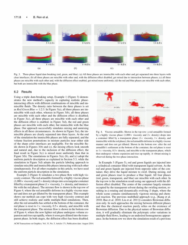
Fig. 3. Three-phase liquid dam breaking (red, green, and blue). (a) All three phases are immiscible with each other and get separated into three layers withclear interfaces; (b) all three phases are miscible with other and, with the diffusion effect disabled, get mixed due to interaction between phases; (c) all threephases are miscible with each other and, with the diffusion effect enabled, get mixed more uniformly; (d) the red and blue phases are miscible with each other,but both are immiscible with the blue phase.

6.2 Results

Using a triple dam-breaking setup, Example 1 (Figure 3) demon-strates the new method’s capacity in capturing realistic phase-interacting effects with different combinations of miscible and im-miscible fluids. The density ratio between the three phases is setas Red:Green:Blue = 1:2:3. In Figure 3(a), all three phases are im-miscible with each other, whereas in Figure 3(b), all three phasesare miscible with each other and the diffusion effect is disabled;in Figure 3(c), all three phases are miscible with each other andthe diffusion effect is enabled; in Figure 3(d), the red and greenphases are miscible with each other, but immiscible with the bluephase. Our approach successfully simulates mixing and unmixingeffects in all these circumstances. As shown in Figure 3(a), the im-miscible phases are clearly separated into three layers. At the endof the simulation the immiscible phases are fully separated, and thevolume fraction penetrations in mixture particles near either sideof the sharp color interfaces are negligible. For the miscible flu-ids shown in Figures 3(b) and (c), the mixing effects look smoothand natural and, due to the inclusion of the diffusion effect, thefinal result in Figure 3(c) is mixed more uniformly than that inFigure 3(b). The simulations in Figures 3(a), (b), and (c) adopt theuniform particle description as explained in Section 5.3, while thesimulation in Figure 3(d) adopts the particle labeling approach tosimulate miscible and immiscible phases interacting with each othersimultaneously. For all other examples in this article, we have usedthe uniform particle description in the simulation.

Example 2 (Figure 4) simulates a two-phase flow with high vis-cosity contrast. The red armadillo formed by a highly viscous phase(1,000× viscosity and 2× density) drops into a rectangular containerfilled by a transparent phase (1× viscosity, 1× density, and immisci-ble with the red phase). The mixture flow is shown in the top row ofFigure 4, where the red armadillo deforms in a highly viscous man-ner and does not get diluted by the transparent phase. This exampleshows our method can cope with very high viscosity contrast andstill achieve realistic and stable multiple-fluid simulations. Then,after the red armadillo has settled at the bottom of the container, thered phase is reset to 1× viscosity, 0.5× density, and miscible withthe transparent phase. The mixture flow is shown in the bottom rowof Figure 4, where the now lighter red phase undergoes volume ex-pansion and rises up rapidly, where it soon gets diluted into the trans-parent phase. In both stages, the diffusion effect has been disabled.

Fig. 4. Viscous armadillo. Shown in the top row: a red armadillo formedby a highly viscous phase (1,000× viscosity and 2× density) drops intoa container filled by a transparent phase (1× viscosity, 1× density, andimmiscible with the red phase); the red armadillo deforms in a highly viscousmanner and does not get diluted. Shown in the bottom row: after the redarmadillo’s settlement at the bottom of the container, the red phase is resetto 1× viscosity, 0.5× density, and miscible to the transparent phase, whichthen undergoes volume expansion and rises up rapidly. A vibrant mixing isobserved during the two-phase interaction.

In Example 3 (Figure 5), red and green liquids are injected intoa cylindrical container filled with transparent liquid solvent. As thered and green liquids are injected from opposite sides of the con-tainer, they drive the liquid mixture to swirl. During mixing, redand green phases react to produce a blue liquid. All four phases(red, green, transparent, and blue) are miscible with each other. Inthe top row is the simulation result using our approach with the dif-fusion effect disabled. The center of the container largely remainsoccupied by the transparent solvent during the swirling motion, re-sulting in a rotating and dynamically evolving S shape, where thewhole scene contains simultaneously vigorous mixing and chem-ical reaction. The previous multifluid approach (e.g., [Kang et al.2010; Bao et al. 2010; Liu et al. 2011]) considers Brownian diffu-sion only. In such approaches the mixing between different phasesand thus the chemical reaction purely relies on the existence ofBrownian diffusion. Due to the physical nature of Brownian diffu-sion, it will gradually eliminate the polytropic color variations inmultiple-fluid flows, leading to an undesired homogeneous appear-ance. In the bottom row we show the simulation result of a previous

ACM Transactions on Graphics, Vol. 33, No. 5, Article 171, Publication date: August 2014.

Multiple-Fluid SPH Simulation Using a Mixture Model • 171:9

Fig. 5. Reacting swirl. Red and green liquids are injected from opposite sides into the container filled with transparent solvent, causing the mixture to swirl.Upon meeting, the red and green liquids react to produce a blue liquid. All four phases are miscible with each other. Top row: Our method, with the diffusioneffect disabled, forms a rotating and dynamically evolving S symbol at the centre of the container, while the whole scene contains simultaneously vigorousmixing and chemical reaction. Bottom row: Using only Brownian diffusion to simulate mixing [Kang et al. 2010; Bao et al. 2010; Liu et al. 2011] results in ahomogeneous appearance.

Fig. 6. Unmixing. Four immiscible liquids (red, yellow, green, and blue)are artificially set to a “fully mixed” state in a circular container with arotating turbine at the centre. During spinning they get “fully separated” dueto the centrifugal effect. Top: perspective view. Bottom: top view.

multifluid approach, where the polytropic color variations graduallyattain a homogeneous appearance. It is clear in this example thatour approach is able to avoid the undesired variation eliminatingeffect and the homogeneous appearance due to Brownian diffu-sion, while simultaneously keeping vigorous mixing and reactionfeaturing polytropic colors throughout the whole simulation.

Example 4 (Figure 6) demonstrates an unmixing process takingplace in a disk-shaped container that has a spinning turbine installedat its centre. The container is filled with four immiscible phaseswith the density ratio Red:Yellow:Green:Blue = 1:1.5:2.5:3, and themixture occupies about 3/4 of the volume. Initially, the four phasesare set at a “fully mixed” state, resulting in a greyish color, andare unmixed due to the centrifugal effect during spinning, resultingin a colorful ring-shaped pattern. The top row in Figure 6 shows aperspective view of this unmixing process, while the bottom rowshows the top view. The gravity force is not considered in thisexample. This unmixing effect cannot be captured by multiple-fluidsimulations where only the diffusion effect is modeled, and also it ishard to achieve through the inter-facial-flow simulation approach.

Example 5 (Figure 7) simulates a four-phase vaporization processwith high-density contrast. A dome is filled with transparent air andtwo liquids (red and green) are injected into the dome from twomagic sources. The red and green liquids meet at the centre of thefloor and react to produce a vapor phase that rises up towards the

Fig. 7. Vaporization. The dome is filled with transparent air and, fromtwo magic sources, red and green liquids are injected into the dome. Thetwo liquids meet at the centre of the floor and react to produce a vaporphase that rises towards the ceiling. The density ratio is Red liquid:Greenliquid:Transparent air:Vapor phase = 1000:1000:2:1.

ceiling. In this example, all four phases are immiscible with eachother and their density ratio is Red liquid:Green liquid:Transparentair:Vapor phase = 1000:1000:2:1. Under high-density contrast, thevaporization process is successfully simulated.

In Example 6 (Figure 8), a tank with a movable wall on the leftis filled with transparent liquid. To the left of the tank, there arefour “reacting regions” marked in red, yellow, blue, and purple.Upon entering these reacting regions, the transparent liquid reactsto produce a new liquid with the color of the region. The wall on theleft moves back and forth periodically to drive the liquid mixtureto flow in the tank. Three more chemical reactions are introduced:the red liquid reacting with the yellow liquid to produce an orangeliquid, the yellow liquid reacting with the blue liquid to producea green liquid, and the blue liquid reacting with the purple liquidto produce an indigo liquid. All eight phases are set as misciblewith each other, thus the mixing flow in the tank creates a livelyrainbow wave with seven naturally colored streams adjacent to each

ACM Transactions on Graphics, Vol. 33, No. 5, Article 171, Publication date: August 2014.

171:10 • B. Ren et al.

Fig. 8. Rainbow wave. The transparent liquid is propelled by the periodically moving wall on the left and, when the transparent liquid passes over the fourmagic regions in the left of the tank, it reacts to produce four new phases (red, yellow, blue, and purple). The adjacent new phases can also react with eachother to produce another three phases (orange, green, and indigo). All eight phases are miscible with each other and the diffusion effect is disabled. A livelyrainbow wave is formed in the tank.

other: red, orange, yellow, green, blue, indigo, and purple. Again,the diffusion effect is disabled in this example to avoid a stiff anduniform appearance.

7. CONCLUSION AND DISCUSSION

By combining the mixture model in computational fluid dynam-ics and the SPH method, we have developed a novel simulationapproach for multiple-fluid flows. Verified in various numericalexperiments, the new approach is versatile and can simultane-ously capture a wide range of multiple-fluid phenomena, includingmixing/unmixing of miscible and immiscible fluids, diffusion andchemical reaction, etc. The new method is robust and can achievestable and realistic simulation under widely varying parameter set-tings, including high viscosity and density contrast. Implementa-tion of our new scheme is straightforward as an extension to ex-isting single-phase fluid simulators. Moreover, the multiple-fluidsimulation can be easily set up with a minimum requirement ofmultiple-fluid information and without unnecessary parameter tun-ing. Compared to the simple diffusion model (e.g., [Kang et al.2010; Bao et al. 2010; Liu et al. 2011]), the proposed approachcaptures a wider range of multiple-fluid phenomena, thus allow-ing efficient production of various interesting and visually real-istic multiple-fluid results with fine details throughout the wholesimulation.

SPH simulations commonly assume constant particle mass overtime and in cases of vaporization this can lead to dramatic increasesof the effective volume of particles due to large density drop, whichsequentially degrades the simulation resolution. To maintain thesimulation resolution, one possible extension to this work wouldbe to introduce an efficient, adaptive refinement strategy to splitthe SPH particles. Another possible future work is to incorporate theenergy equation into the current theoretical framework to simulaterelatively less commonly observed energy-related effects, such asextraction in chemistry.

Previous numerical strategies that enforce the incompressibilitybased on the divergence-free property of the flow field cannot bedirectly applied to the multiple-fluid simulation, since neither thedivergence of the mixture velocity nor that of the phase velocityis zero, even when all phases are incompressible. At the cost ofsmaller time steps, this limitation can be partially overcome by in-creasing the gas constant in the equations of state to a higher value,but it will be beneficial to investigate new pressure correction meth-ods enforcing incompressibility of the multiple-fluid simulation atlarger time steps, where component-wise incompressibility rela-tions should be taken into account. Another challenge is that incor-porating the mixture model with the Predictive-Corrective Incom-pressible SPH (PCISPH) is not straightforward. PCISPH presumes

uniform particle mass and rest density between particles, how-ever, these properties usually vary between particles in the mixturemodel. This makes the precomputation in the pressure correctionof PCISPH impossible, resulting in erroneous values where there isparticle deficiency.

APPENDIX

APPENDIX A. DERIVATION OF EQNS. (17–19)

This appendix shows the detailed derivations of Eqs. (17)–(19). TheSPH approximation for the divergence operator can be expressed as[Colagrossi and Landrini 2003]

(∇ · A)i =∑

j

dVj Aj · ∇Wij =∑

j

dVj (Aj ± Ai) · ∇Wij . (35)

Eq. (18) and Eq. (19) are direct results following Eq. (35).The derivation of Eq. (17) is more involved. Applying standard

SPH formulation to the right-hand side of the following identity

(αk∇ · um)i = (∇ · (αkum))i − (um · ∇αk)i (36)

leads to

(αk∇ · um)i =∑

j

dVjαkj (umj − umi) · ∇Wij . (37)

However, applying Eq. (35) to the left-hand side of Eq. (36) yields:

(αk∇ · um)i =∑

j

dVjαki(umj − umi) · ∇Wij . (38)

The two preceding equations are almost the same, and directlyaveraging the right-hand side yields Eq. (17).

ACKNOWLEDGMENTS

The authors would like to thank the anonymous reviewers for theirconstructive comments.

REFERENCES

R. Ando and R. Tsuruno. 2010. Vector fluid: A vector graphics depictionof surface flow. In Proceedings of the 8th International Symposium onNon-Photorealistic Animation and Rendering (NPAR’10). ACM Press,New York, 129–135.

K. Bao, X. Wu, H. Zhang, and E. Wu. 2010. Volume fraction based miscibleand immiscible fluid animation. Comput. Animat. Virtual Worlds 21, 3–4,401–410.

ACM Transactions on Graphics, Vol. 33, No. 5, Article 171, Publication date: August 2014.

Multiple-Fluid SPH Simulation Using a Mixture Model • 171:11

M. Becker and M. Teschner. 2007. Weakly compressible SPH for free surfaceflows. In Proceedings of the ACM SIGGRAPH/Eurographics Symposiumon Computer Animation (SCA’07). Eurographics Association, 209–217.

L. Boyd and R. Bridson. 2012. Multiflip for energetic two-phase fluid sim-ulation. ACM Trans. Graph. 31, 2, 16:1–16:12.

O. Busaryev, T. K. Dey, H. Wang, and Z. Ren. 2012. Animating bubbleinteractions in a liquid foam. ACM Trans. Graph. 31, 4, 63:1–63:8.

P. W. Cleary. 1996. New implementation of viscosity: Tests with couetteflows. Tech. rep. DMS-C96/32, CSIRO Division of Math and Statistics.

P. W. Cleary, S. H. Pyo, M. Prakash, and B. K. Koo. 2007. Bubbling andfrothing liquids. ACM Trans. Graph. 26, 3.

A. Colagrossi and M. Landrini. 2003. Numerical simulation of interfacialflows by smoothed particle hydrodynamics. J. Comput. Phys. 191, 2,448–475.

C. T. Crowe, J. D. Schwarzkopf, M. Sommerfeld, and Y. Tsuji. 2011. Mul-tiphase Flows with Droplets and Particles. CRC Press, Boca Raton, FL.

F. Dagenais, J. Gagnon, and E. Paquette. 2012. A prediction-correction ap-proach for stable SPH fluid simulation from liquid to rigid. In Proceedingsof the Computer Graphics International.

M. Desbrun and M. Paule Gascuel. 1996. Smoothed particles: A newparadigm for animating highly deformable bodies. In Proceedings ofthe Eurographics Workshop on Computer Animation and Simulation.Springer, 61–76.

L. M. Gonzalez, J. M. Sanchez, F. Macia, and A. Souto-Iglesias. 2009.Analysis of WCSPH laminar viscosity models. In Proceedings of the 4th

ER-COFTAC SPHERIC Workshop on SPH Applications.

J. Gregson, M. Krimerman, M. B. Hullin, and W. Heidrich. 2012. Stochastictomography and its applications in 3D imaging of mixing fluids. ACMTrans. Graph. 31, 4, 52:1–52:10 (to appear).

J.-M. Hong and C.-H. Kim. 2005. Discontinuous fluids. ACM Trans. Graph.24, 3, 915–920.

J.-M. Hong, H.-Y. Lee, J.-C. Yoon, and C.-H. Kim. 2008. Bubbles alive.ACM Trans. Graph. 27, 3, 48:1–48:4.

X. Hu and N. Adams. 2006. A multi-phase {SPH} method for macroscopicand mesoscopic flows. J. Comput. Phys. 213, 2, 844–861.

I. Ihm, B. Kang, and D. Cha. 2004. Animation of reactive gaseousfluids through chemical kinetics. In Proceedings of the ACM SIG-GRAPH/Eurographics Symposium on Computer Animation. EurographicsAssociation, 203–212.

M. Ihmsen, N. Akinci, G. Akinci, and M. Teschner. 2012. Unified spray,foam and air bubbles for particle-based fluids. Vis. Comput. 28, 6–8,669–677.

B. Kang, Y. Jang, and I. Ihm. 2007. Animation of chemically reactive flu-ids using a hybrid simulation method. In Proceedings of the ACM SIG-GRAPH/Eurographics Symposium on Computer Animation. EurographicsAssociation, 199–208.

N. Kang, J. Park, J. Noh, and S. Y. Shin. 2010. A hybrid approach tomultiple fluid simulation using volume fractions. Comput. Graph. Forum29, 2, 685–694.

R. Keiser, B. Adams, D. Gasser, P. Bazzi, P. Dutre, and M. Gross. 2005. Aunified lagrangian approach to solid-fluid animation. In Proceedings ofthe 2nd Eurographics/IEEE/VGTC Conference on Point-Based Graphics(SPBG’05). Eurographics Association, 125–133.

B. Kim. 2010. Multi-phase fluid simulations using regional level sets. ACMTrans. Graph. 29, 6, 175:1–175:8.

B. Kim, Y. Liu, I. Llamas, X. Jiao, and J. Rossignac. 2007. Simulation of bub-bles in foam with the volume control method. ACM Trans. Graph. 26, 3.

D. Kim, O.-Y. Song, and H.-S. Ko. 2010. A practical simulation of dispersedbubble flow. ACM Trans. Graph. 29, 70:1–70:5.

P.-R. Kim, H.-Y. Lee, J.-H. Kim, and C.-H. Kim. 2012. Controlling shapesof air bubbles in a multi-phase fluid simulation. Vis. Comput. 28, 6–8,597–602.

N. I. Kolev. 2005. Multiphase Flow Dynamics 1: Fundamentals. Springer.S. Liu, Q. Liu, and Q. Peng. 2011. Realistic simulation of mixing fluids.

Vis. Comput. 27, 3, 241–248.F. Losasso, T. Shinar, A. Selle, and R. Fedkiw. 2006. Multiple interacting

liquids. ACM Trans. Graph. 25, 3, 812–819.M. Manninen, V. Taivassalo, and S. Kallio. 1996. On the mixture model for

multiphase flow. http://www.vtt.fi/inf/pdf/publications/1996/P288.pdf.V. Mihalef, B. Unlusu, D. Metaxas, M. Sussman, and M. Y. Hussaini.

2006. Physics based boiling simulation. In Proceedings of the ACM SIG-GRAPH/Eurographics Symposium on Computer Animation (SCA’06).Eurographics Association, 317–324.

M. K. Misztal, K. Erleben, A. Bargteil, J. Fursund, B. B. Christensen, J.A. Bærentzen, and R. Bridson. 2012. Multiphase flow of immisciblefluids on unstructured moving meshes. In Proceedings of the ACM SIG-GRAPH/Eurographics Symposium on Computer Animation (SCA’12).Eurographics Association, 97–106.

J. Monaghan. 1992. Smoothed particle hydrodynamics. Ann. Rev. Astron.Astrophys. 30, 543–574.

J. J. Monaghan and A. Rafiee. 2013. A simple sph algorithm for multi-fluidflow with high density ratios. Int. J. Numer. Methods Fluids 71, 5,537–561.

P. Mullen, A. McKenzie, Y. Tong, and M. Desbrun. 2007. A variationalapproach to eulerian geometry processing. ACM Trans. Graph. 26, 3.

M. Muller, D. Charypar, and M. Gross. 2003. Particle-based fluidsimulation for interactive applications. In Proceedings of the ACM SIG-GRAPH/Eurographics Symposium on Computer Animation (SCA’03).Eurographics Association, 154–159.

M. Muller, B. Solenthaler, R. Keiser, and M. Gross. 2005. Particle-based fluid-fluid interaction. In Proceedings of the ACM SIGGRAPH/Eurographics Symposium on Computer Animation (SCA’05). ACMPress, New York, 237–244.

M. B. Nielsen and O. Osterby. 2013. A two-continua approach to euleriansimulation of water spray. ACM Trans. Graph. 32, 4, 67:1–67:10.

J. Park, Y. Kim, D. Wi, N. Kang, S. Y. Shin, and J. Noh. 2008. A unifiedhandling of immiscible and miscible fluids. Comput. Animat. VirtualWorlds 19, 3–4, 455–467.

S. Premoze, T. Tasdizen, J. Bigler, A. E. Lefohn, and R. T. Whitaker.2003. Particle-based simulation of fluids. Comput. Graph. Forum 22, 3,401–410.

B. Solenthaler and R. Pajarola. 2008. Density contrast sph interfaces.In Proceedings of the ACM SIGGRAPH/Eurographics Symposium onComputer Animation (SCA’08). Eurographics Association, 211–218.

B. Solenthaler, J. Schlafli, and R. Pajarola. 2007. A unified particle modelfor fluid-solid interactions: Research articles. Comput. Animat. VirtualWorlds 18, 1, 69–82.

G. H. Yeoh and J. Tu. 2009. Computational Techniques for MultiphaseFlows. Butterworth-Heinemann.

H. Zhu, X. Liu, Y. Liu, and E. Wu. 2006. Simulation of miscible binarymixtures based on lattice boltzmann method: Research articles. Comput.Animat. Virtual Worlds 17, 3–4, 403–410.

Received September 2013; revised March 2014; accepted April 2014

ACM Transactions on Graphics, Vol. 33, No. 5, Article 171, Publication date: August 2014.