1

Multiple Context-Free Grammars: Basic Properties and Complexity

Hiroyuki Seki

NAIST

MCFG+2

Nara, Sept 9, 2011

2

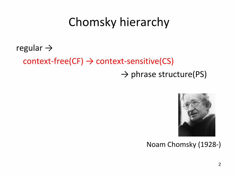
Chomsky hierarchy

regular →

context-free(CF) → context-sensitive(CS)

→ phrase structure(PS)

Noam Chomsky (1928-)

3

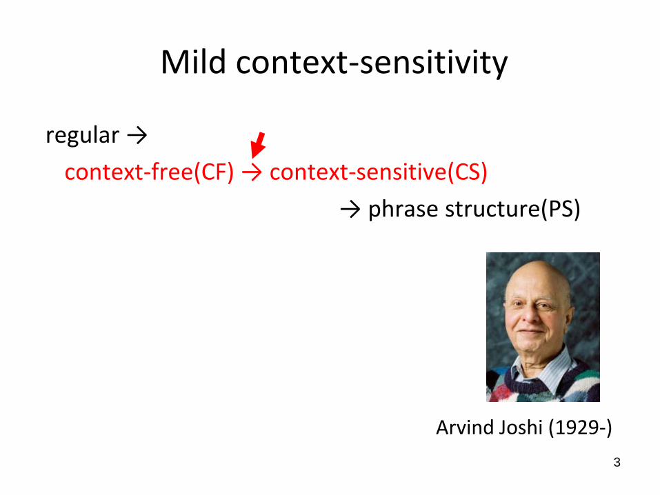
Mild context-sensitivity

regular →

context-free(CF) → context-sensitive(CS)

→ phrase structure(PS)

Arvind Joshi (1929-)

Macro grammar (Fischer 1968) Indexed grammar (Aho 1968) CF tree grammar (Rounds 1970)

Tree Adjoining Grammar (Joshi, Levy & Takahashi 1975)

Tree transducer (Engelfriet+)

Linear CF rewriting system (Vijay-Shanker, Weir & Joshi 1987) = Multiple CF grammar (Kasami, Seki & Fujii 1987),

Crossed interaction grammar (Rivas & Eddy 2000)

… … 1970 1980 1990 2000

Description of Natural Language Syntax

Syntax-Directed Translation

Biological Sequence Analysis

4

5

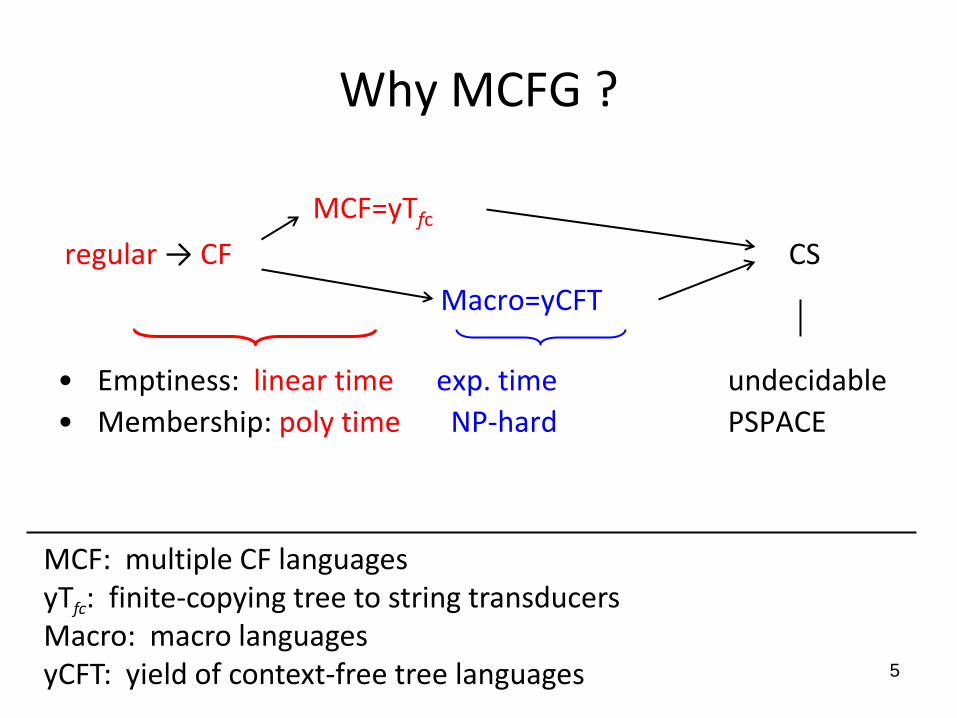
Why MCFG ?

MCF=yTfc regular → CF CS Macro=yCFT

• Emptiness: linear time exp. time undecidable • Membership: poly time NP-hard PSPACE

MCF: multiple CF languages yTfc: finite-copying tree to string transducers Macro: macro languages yCFT: yield of context-free tree languages

MCFG

• Kasami, Seki & Fujii, Tech. Rep., Osaka U. 1987, also in IEICE Trans., J71-D-I(5,6), 1988.

• Seki, Matsumura, Fujii & Kasami, TCS 88(2), 1991.

• Seki, Nakanishi, Kaji, Ando & Kasami, 31st ACL, 130-139, 1993.

• Kaji, Nakanishi, Seki & Kasami, Computational Intelligence, 10(4), 440-452, 1994., etc.

Tadao Kasami (1930-2007)

6

Contents

• Definitions

• Basic properties

• Recognition complexity

• Appendix

7

8

CFG as a set of clauses

CFG DHC (Definite Horn Clause) Nonterminal ⇔ Unary predicate A symbol A A(x) “A can derive x.” rules ⇔ clauses A → B C A(xy) :- B(x), C(y). A → a A(a). (B⇒*u and C⇒*v) ( B(u) and C(v) ) implies A⇒*uv . ⇔ implies A(uv) .

9

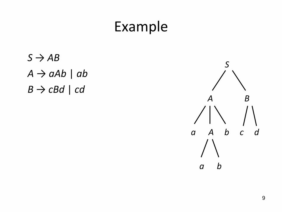
Example

S → AB

A → aAb | ab

B → cBd | cd

S A B a A b c d a b

10

Example

S(xy) :- A(x), B(y).

A(axb) :- A(x). A(ab).

B(cxd) :- B(x). B(cd).

Derivation of aabbcd from S

= Proof of S(aabbcd).

S(aabbcd) A(aabb) B(cd) A(ab)

11

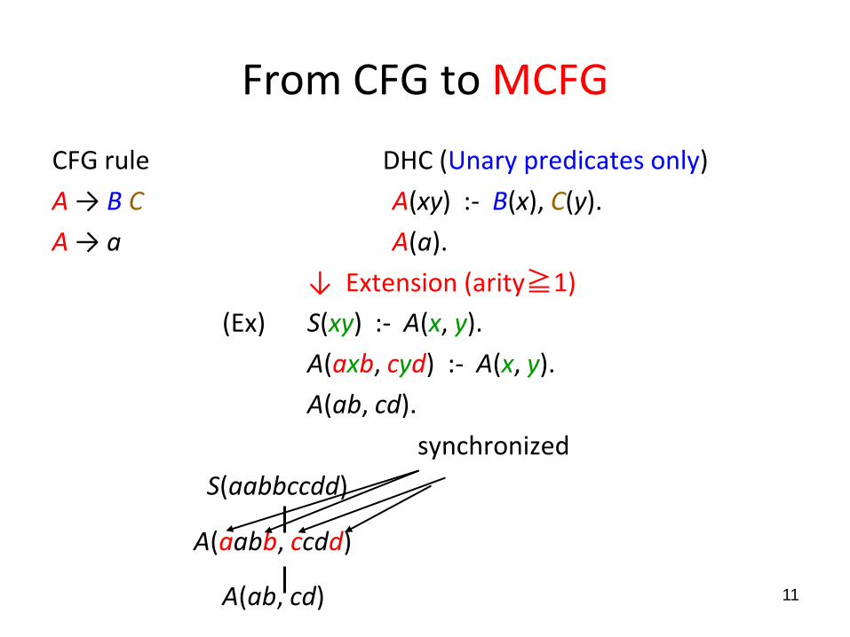
From CFG to MCFG

CFG rule DHC (Unary predicates only)

A → B C A(xy) :- B(x), C(y).

A → a A(a).

↓ Extension (arity≧1) (Ex) S(xy) :- A(x, y).

A(axb, cyd) :- A(x, y).

A(ab, cd).

synchronized S(aabbccdd)

A(aabb, ccdd)

A(ab, cd)

12

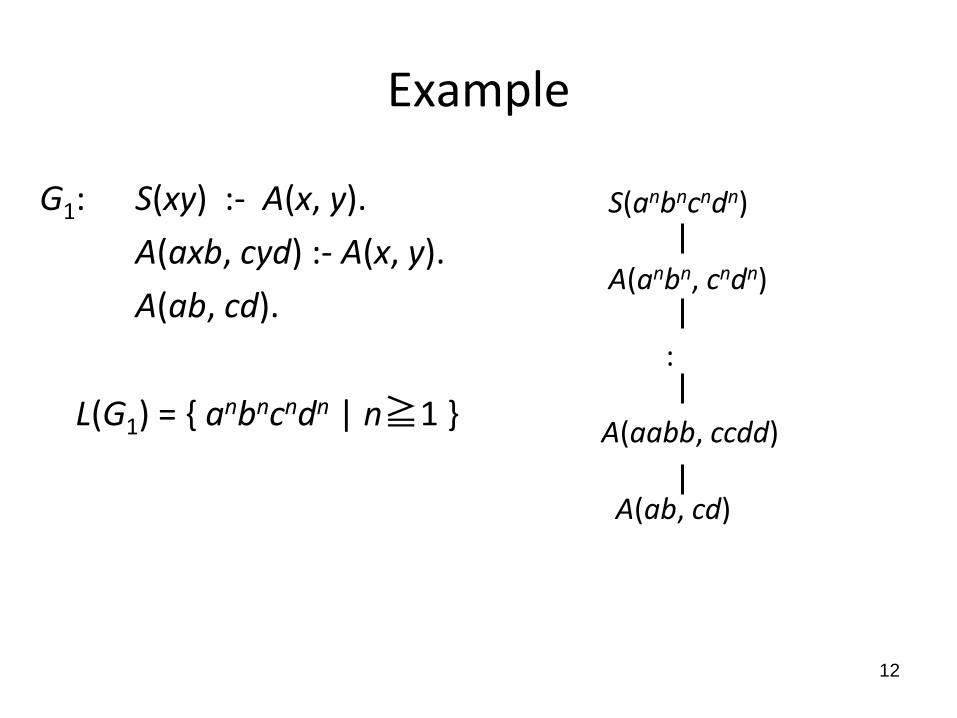
Example

G1: S(xy) :- A(x, y).

A(axb, cyd) :- A(x, y).

A(ab, cd).

L(G1) = { anbncndn | n≧1 }

S(anbncndn) A(anbn, cndn) : A(aabb, ccdd) A(ab, cd)

13

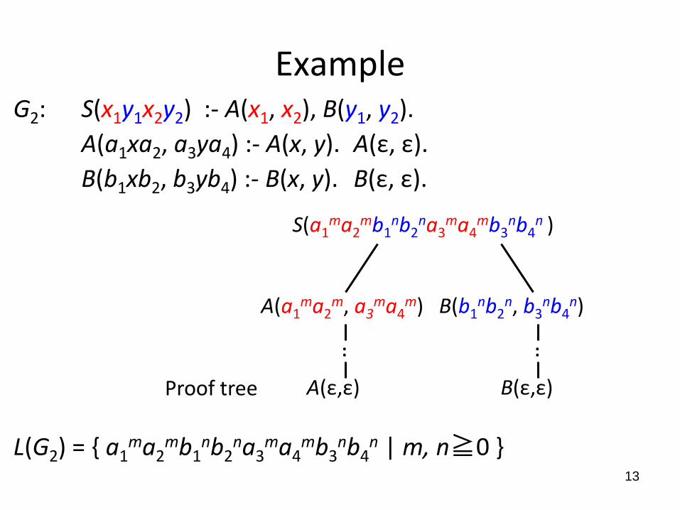
Example G2: S(x1y1x2y2) :- A(x1, x2), B(y1, y2).

A(a1xa2, a3ya4) :- A(x, y). A(ε, ε). B(b1xb2, b3yb4) :- B(x, y). B(ε, ε).

L(G2) = { a1ma2

mb1nb2

na3ma4

mb3nb4

n | m, n≧0 }

S(a1ma2

mb1nb2

na3ma4

mb3nb4

n ) A(a1

ma2m, a3

ma4m) B(b1

nb2n, b3

nb4n)

A(ε,ε) B(ε,ε) Proof tree

: :

14

MCFG

G=(N, T, V, P, S) N: predicates (nonterminals), T: terminals, V: variables, P: rules, S∈N: start predicate • A rule π ∈ P is a definite Horn clause s.t.

– Both head & body are linear (w. r. t. V), – Argument of predicate in body is variable, – Argument of predicate in head is string over T and variables in its body.

(Ex) A(axb, cyd) :- A(x, y). B(x1y1, x2y2) :- C(x1, x2), D(y1, y2). NG A(x, ax) :- B(x). NG A(x, y) :- B(x, y), C(x).

15

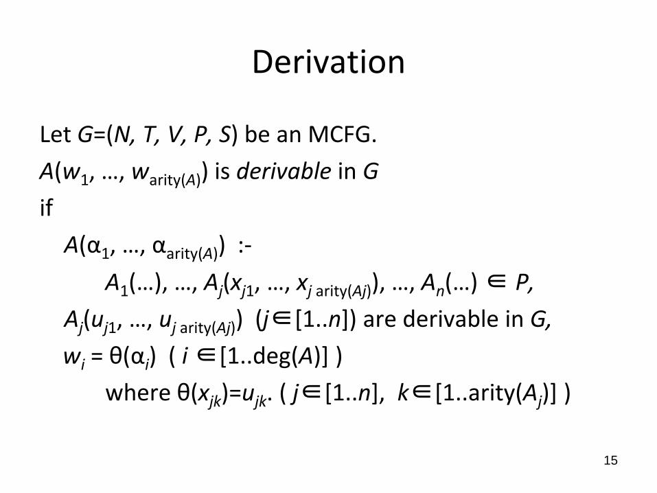
Derivation

Let G=(N, T, V, P, S) be an MCFG.

A(w1, …, warity(A)) is derivable in G

if

A(α1, …, αarity(A)) :-

A1(…), …, Aj(xj1, …, xj arity(Aj)), …, An(…) ∈ P,

Aj(uj1, …, uj arity(Aj)) (j∈[1..n]) are derivable in G,

wi = θ(αi) ( i ∈[1..deg(A)] )

where θ(xjk)=ujk. ( j∈[1..n], k∈[1..arity(Aj)] )

16

MCFG Language

For an MCFG G=(N, T, V, P, S),

L(G) := { w∈T* | S(w) is derivable in G } is the multiple context-free language (mcfl) generated

by G.

17

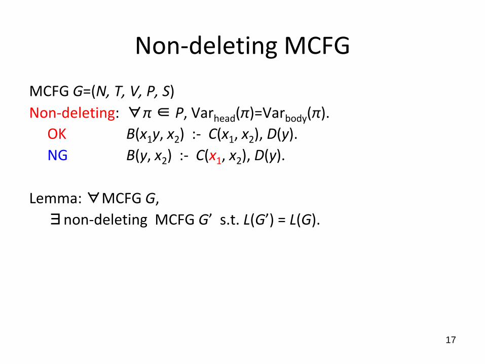
Non-deleting MCFG

MCFG G=(N, T, V, P, S) Non-deleting: ∀π ∈ P, Varhead(π)=Varbody(π). OK B(x1y, x2) :- C(x1, x2), D(y). NG B(y, x2) :- C(x1, x2), D(y). Lemma: ∀MCFG G, ∃non-deleting MCFG G’ s.t. L(G’) = L(G).

18

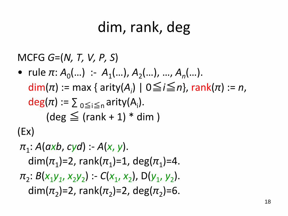
dim, rank, deg

MCFG G=(N, T, V, P, S) • rule π: A0(…) :- A1(…), A2(…), …, An(…). dim(π) := max { arity(Ai) | 0≦i≦n}, rank(π) := n, deg(π) := ∑ 0≦i≦n arity(Ai). (deg ≦ (rank + 1) * dim ) (Ex) π1: A(axb, cyd) :- A(x, y). dim(π1)=2, rank(π1)=1, deg(π1)=4. π2: B(x1y1, x2y2) :- C(x1, x2), D(y1, y2). dim(π2)=2, rank(π2)=2, deg(π2)=6.

19

dim, rank, deg (cnt’d)

For MCFG G=(N, T, V, P, S), {dim, rank, deg}(G) := maxπ∈P {dim, rank, deg}(π) • q-MCFG(r): MCFG with dim≦q and rank≦r • q-MCFG: MCFG with dim≦q • MCFG(r): MCFG with rank≦r

20

Notation

(Class of)

Grammars

CFG MCFG q-MCFG(r) …

(Class of)

Languages

CFL MCFL q-MCFL(r) …

21

Properties of MCFG (Also see [Vijay-Shanker, Weir & Joshi 1987])

• (Generative power) CFL ⊆ MCFL ⊆ CSL. • Every MCFL is semilinear. • (Closure property)

– full AFL. – Not closed under intersection.

• (Decidability) – Emptiness (L(G)=Φ?): O(|G|)-time decidable. – Recognition (w∈L(G)?): poly-time decidable. – Inclusion (L(G1)⊆L(G2)?) : Undecidable.

full AFL : a class of languages closed by homomorphism, inv. homomorphism, intersection with regular sets, union, Kleene closure

Proof example (exercise)

(Closure under intersection with regular language.)

CFL case:

For given CFG in Chomsky normal form G=(N, T, P, S) &

FA (finite automaton) M=(Q, T, δ, p0, F)

(Q: set of states, δ: transition function, p0: initial state, F: set of final states),

construct CFG G’=(N×Q×Q∪{S’}, T, P’, S’) where

22

∩R Closure: CFG Case

• ∀A→BC∈P, ∀q1, q2, q3 ∈Q :

A[q1,q3] → B[q1,q2] C[q2,q3] ∈P’

• ∀A→a∈P, ∀q1, q2∈Q s.t. δ(q1, a)=q2:

A[q1,q2] → a∈P’

Correctness:

A[q1,q2] ⇒*G’ w iff

A ⇒*G w and δ*(q1, w)=q2

23

∩R Closure: MCFG Case (1/2)

A(x1y1, y2x2) :- B(x1, x2), C(y1, y2) ∈P A[?, ?, ?, ?] (x1y1, y2x2) :-

B[q1,q2,q3,q4] (x1, x2), C[r1,r2,r3,r4] (y1, y2) ∈P’

A[q1,r2,r3,q4] (x1y1, y2x2) :-

B[q1,q2,q3,q4] (x1, x2), C[q2,r2,r3,q3] (y1, y2) ∈P’

24

x1 x2 y2 y1

q１ q2=r1 r2 r3 r4=q3 q4

∩R Closure: MCFG Case (2/2)

Correctness:

A[q1s,q1e,…,qns,qne](w1,…,wn) provable in G’ iff

A(w1,…,wn) derivable in G

and

δ*(qjs, w)=qje (j∈[1..n])

25

26

Properties of q-MCFG(r)

• q-MCFL(r), MCFL(r), q-MCFL (r≧2, q≧1): substitution closed full AFL.

• q-MCFL = yT FIN(q) [Weir92]

(yield of tree transducers with copy bound q)

• q-MCFL(1) = ET0L FIN(q)

(DT0L with copy bound q)

• TAL ⊆2-MCFL(2)

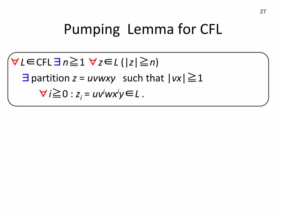
Pumping Lemma for CFL

∀L∈CFL∃n≧1 ∀z∈L (|z|≧n)

∃partition z = uvwxy such that |vx|≧1

∀i≧0 : zi = uviwxiy∈L .

27

Pumping Lemma for MCFL

For general MCFL :

∀L∈q-MCFL∃n≧1 ∃ z∈L (|z|≧n)

∃partition z = u1v1w1s1u2…uqvqwqsquq+1 Σ|vjsj|≧1

∀i≧0 : zi = u1v1iw1s1

iu2…uqvqiwqsq

iuq+1∈L . For well-nested MCFL [Ka09] :

∀L∈q-wnMCFL ∃n≧1 ∀z∈L (|z|≧n)

∃partition z = … (same as above) …

∀i≧0 : zi = u1v1iw1s1

iu2…uqvqiwqsq

iuq+1∈L .

28

[Ka09] Kanazawa, The pumping lemma for well-nested multiple context-free languages, DLT09, LNCS 5583.

Recently, it was proved that the strong version

does not hold for general MCFL.

Pumping lemma

29

A(w1, w2)

A(aaw1bb, ccw2dd)

An easy case. u1v1

i w1 s1i u2 v2

i w2 s2i u3 ∈L

A(aw1b, cw2d)

A(aw1b, cw2d)

A(w1, w2)

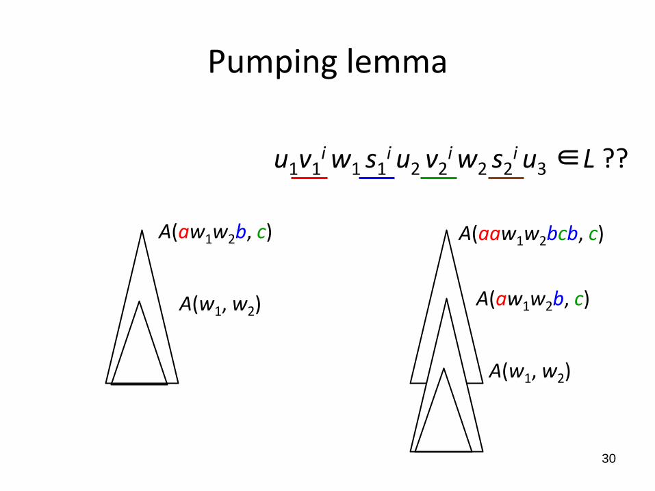
Pumping lemma

30

A(w1, w2)

A(aw1w2b, c)

A(w1, w2)

A(aaw1w2bcb, c)

A(aw1w2b, c)

u1v1i w1 s1

i u2 v2i w2 s2

i u3 ∈L ??

31

Hierarchy on dimensions

dim q =1 2 3 4 5 :

rank r ≧1

Infinite hierarchy

CFL { a1na2

n | n≧0 }

{ a1na2

na3na4

n | n≧0 }

{ a1na2

na3na4

na5na6

n | n≧0 }

…

32

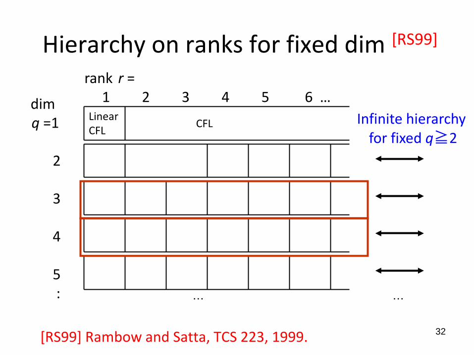
Hierarchy on ranks for fixed dim [RS99]

[RS99] Rambow and Satta, TCS 223, 1999.

dim q =1 2 3 4 5 :

rank r = 1 2 3 4 5 6 …

Linear CFL

CFL

… …

Infinite hierarchy for fixed q≧2

33

Hierarchy on ranks [RS99][Matsumura89]

dim q≧1

rank r = 1 2 3 4 5 6 …

= = = = =

MCFL=MCFL(2) ⇒ It suffices to consider MCFL(1) and MCFL(2) as far as ranks are concerned.

Two layers

34

Trade-offs [RS99]

rank r 1 2 3 4 5 6 dim

q = 1

2

3

4

5

6

7

8

9

10

LCFL CFL q-MCFL(r)⊆ (k+1)q-MCFL(r-k) Corollary: q-MCFL(r)⊆ (r-1)q-MCFL(2)

35

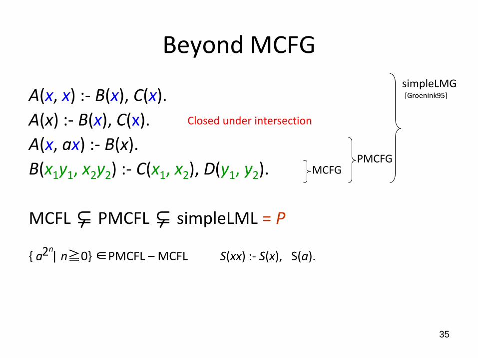
Beyond MCFG

A(x, x) :- B(x), C(x). A(x) :- B(x), C(x). A(x, ax) :- B(x). B(x1y1, x2y2) :- C(x1, x2), D(y1, y2). MCFL ⊆ PMCFL ⊆ simpleLML = P { a | n≧0} ∈PMCFL – MCFL S(xx) :- S(x), S(a).

MCFG PMCFG

simpleLMG [Groenink95]

Closed under intersection

2n

36

Other topics on MCFG (Also refer to the other talks.)

• Parsing

– Earley type parser (Matsumura+89), (Kanazawa 08)

– ‘Unambiguous’ MCFG (O(n2) time recognizable) (Nakanishi92)

– LL(k) MCFG (Nii96)

– Stochastic CYK parser (Kato+06)

• An extension of Chomsky-Schuzenberger theorem for CFL (Kaji+91, Yoshinaka+10)

37

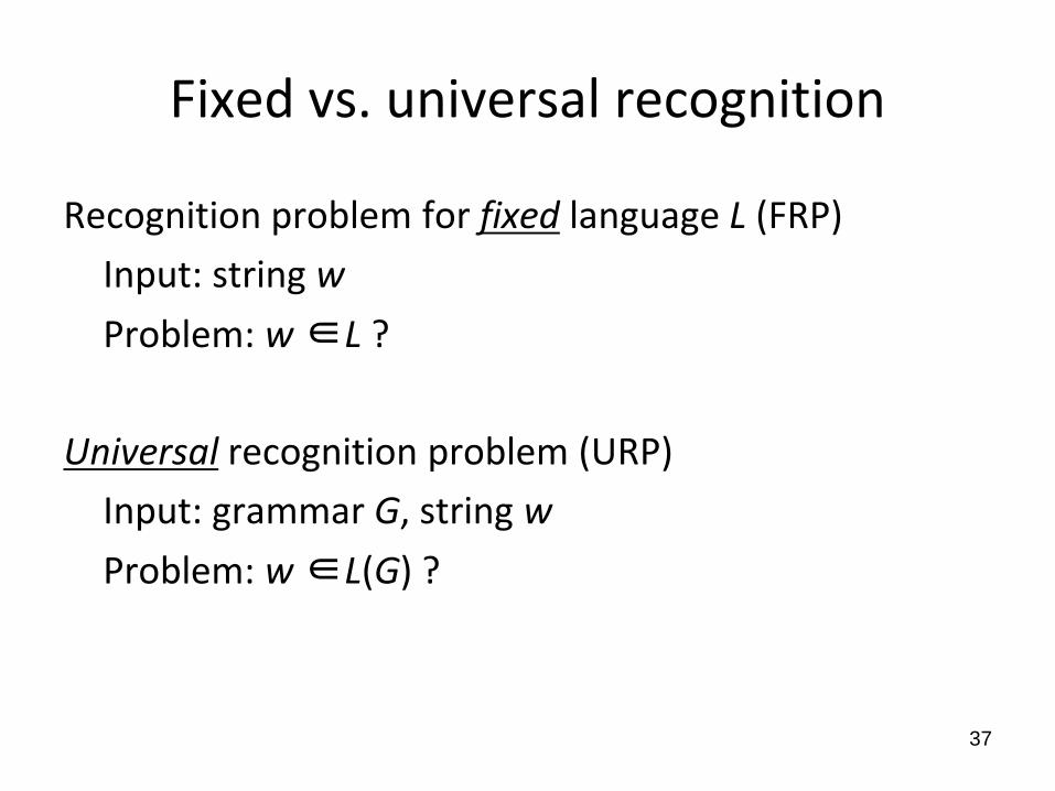
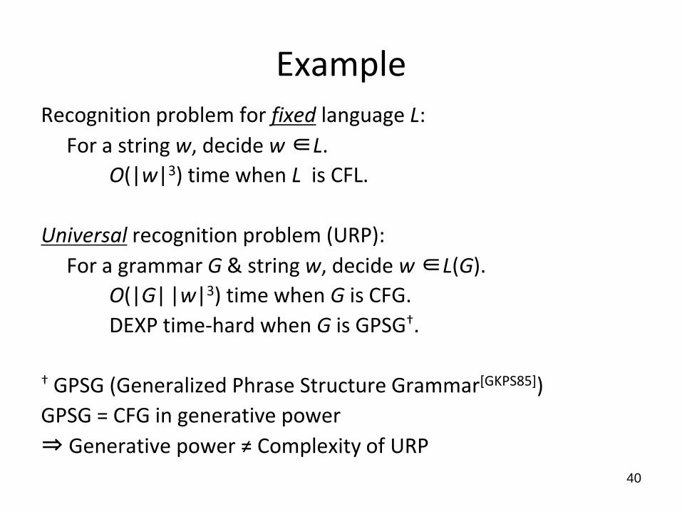
Fixed vs. universal recognition

Recognition problem for fixed language L (FRP)

Input: string w

Problem: w ∈L ?

Universal recognition problem (URP)

Input: grammar G, string w

Problem: w ∈L(G) ?

38

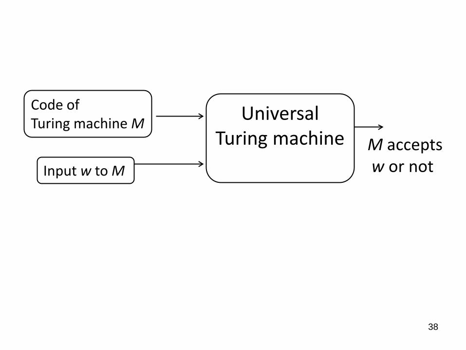
Code of Turing machine M Universal

Turing machine Input w to M

M accepts w or not

URP

39

Description of grammar G Universal

recognition algorithm String w

G generates w or not

40

Example Recognition problem for fixed language L: For a string w, decide w ∈L. O(|w|3) time when L is CFL. Universal recognition problem (URP): For a grammar G & string w, decide w ∈L(G). O(|G| |w|3) time when G is CFG. DEXP time-hard when G is GPSG†.

† GPSG (Generalized Phrase Structure Grammar[GKPS85]) GPSG = CFG in generative power ⇒ Generative power ≠ Complexity of URP

FRP vs. URP

• Generative power can be measured by Complexity of FRP • Generative power ≠ Complexity of URP Rather, complexity of URP for grammar class C ～ Succinctness of C Grammar (especially MCFG) as computation device

with bounded resource Let’s start with FRP.

41

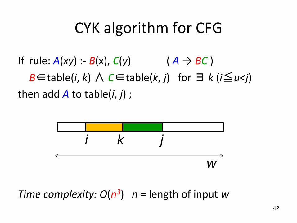
CYK algorithm for CFG

If rule: A(xy) :- B(x), C(y) ( A → BC )

B∈table(i, k) ∧ C∈table(k, j) for ∃ k (i≦u<j) then add A to table(i, j) ;

Time complexity: O(n3) n = length of input w 42

i k j w

CYK algorithm for MCFG

If rule: A(y1z1, z2y2) :- B(y1, y2), C(z1, z2),

B∈table(i, u, v+1, l) ∧ C∈table(u+1, j, k, v)

for ∃ u, v (i≦u<j, k≦v<l) then add A to table(i, j, k, l) ;

• Time complexity: O(ndeg(G)) (deg(G)≦(r+1)q)

(deg(G)=6 in this example) 43

i u j k v l w

44

URP for MCFG

• General case DEXP-complete

• Non-deleting MCFG PSPACE-complete

• q-MCFG with fixed q NP-complete

• q-MCFG(r) with fixed q, r P-complete

General case

• DEXP-complete

– Upper bound: Simulation of MCFG by DEXP time bounded Turing machine.

– Lower bound: Simulation of PSPACE bounded alternating Turing machine (APSPACE) by MCFG.

Since general MCFG can use deleting rules, it can simulate computation for a universal state (of alternating TM) with poly-length ‘sentential form.’

45

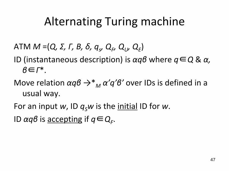
Alternating Turing machine

ATM is M =(Q, Σ, Γ, B, δ, qs, QF, QU, QE)

Q = QU∪QE∪QF∪{qs} : state set

Σ (⊆Γ - {B}): input symbols Γ: tape symbols B: blank symbol

δ⊆(Q×Γ)×(Q×Γ×{→,←}): transition relation qs: initial state QF: final (accepting) states

QU: set of universal states

QE: set of existential states

46

Alternating Turing machine

ATM M =(Q, Σ, Γ, B, δ, qs, QF, QU, QE)

ID (instantaneous description) is αqβ where q∈Q & α, β∈Γ*.

Move relation αqβ →*M α’q’β’ over IDs is defined in a usual way.

For an input w, ID qSw is the initial ID for w.

ID αqβ is accepting if q∈QF.

47

Nondeterministic Turing machine

Input w is accepted if there is a run that reaches an accepting ID from the initial ID for w.

48

accept …

initial ID

Alternating Turing machine For q∈QF, ID αqβ (trivially) is accepting.

For q∈QE, ID αqβ is accepting if there is γ such that αqβ →*M γ and γ is accepting.

For q∈QU, ID αqβ is accepting if every γ satisfying αqβ →*M γ is accepting.

49 accept accept accept accept

∃

∀ ∃

∃ ∀ ∃ ∀

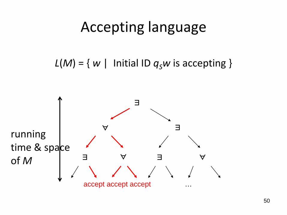
Accepting language

L(M) = { w | Initial ID qSw is accepting }

50

accept accept accept …

∃

∀ ∃

∃ ∀ ∃ ∀

running time & space of M

TM and ATM

APTIME := class of problems solvable by poly time-bounded ATM

APSPACE := class of problems solvable by poly space-bounded ATM

51

Propositon[CS80]: PSPACE=APTIME, DEXPTIME=APSPACE

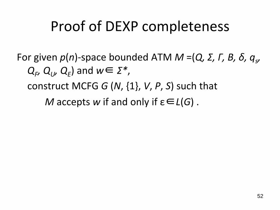
Proof of DEXP completeness

For given p(n)-space bounded ATM M =(Q, Σ, Γ, B, δ, qs, QF, QU, QE) and w∈ Σ*,

construct MCFG G (N, {1}, V, P, S) such that

M accepts w if and only if ε∈L(G) .

52

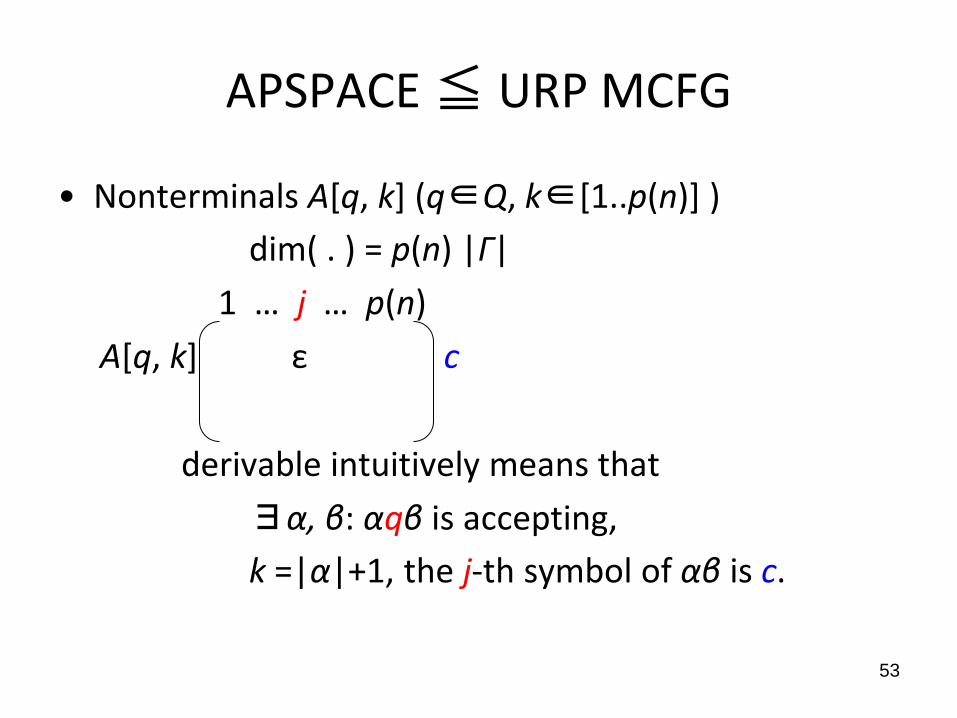
APSPACE ≦ URP MCFG

• Nonterminals A[q, k] (q∈Q, k∈[1..p(n)] ) dim( . ) = p(n) |Γ|

1 … j … p(n)

A[q, k] ε c

derivable intuitively means that

∃α, β: αqβ is accepting, k =|α|+1, the j-th symbol of αβ is c.

53

Construction

(0 step acceptance)

∀qf∈QF, ∀ k∈[1..p(n)] A[qf, k](ε, …, ε) .

(Initial ID)

∀q∈Q, ∀ k∈[1..p(n)] S(x<1,a1>x<2,a2>…x<n,an>x<n+1,B> … x<p(n),B>)

:- A[q, k](…)

for given input w = a1a2…an.

54

Construction (existential state)

• q∈QE, (b, p, →) ∈δ(q, a) (move right) A[q,2] (x<1,a> , x<2,b> , x<3,a> ,

x<1,b> , 1 , x<3,b> ,

x<1,c> , 1 , x<3,c> ) :-

A[p, 3] (x<1,a> , x<2,a> , x<3,a> ,

x<1,b> , x<2,b> , x<3,b> ,

x<1,c> , x<2,c> , x<3,c> )

55

c a ... q

c b ... p

→M

Construction (universal state)

• q∈QU, , (b, p, →) ∈δ(q, a) , (c, r, ←) ∈δ(q, a) A[q,2] (x<1,a> y<1,a> , x<2,b> y<2,c> , x<3,a> y<3,a> ,

x<1,b> y<1,b> , 1 , x<3,b> y<3,b> ,

x<1,c> y<1,c> , 1 , x<3,c> y<3,c> ) :-

A[p , 3] (x<1,a> , x<2,a> , x<3,a> ,

x<1,b> , x<2,b> , x<3,b> ,

x<1,c> , x<2,c> , x<3,c> ),

A[r, 3] (y<1,a> , y<2,a> , y<3,a> ,

y<1,b> , y<2,b> , y<3,b> ,

y<1,c> , y<2,c> , y<3,c> ), 56

Recent result

57

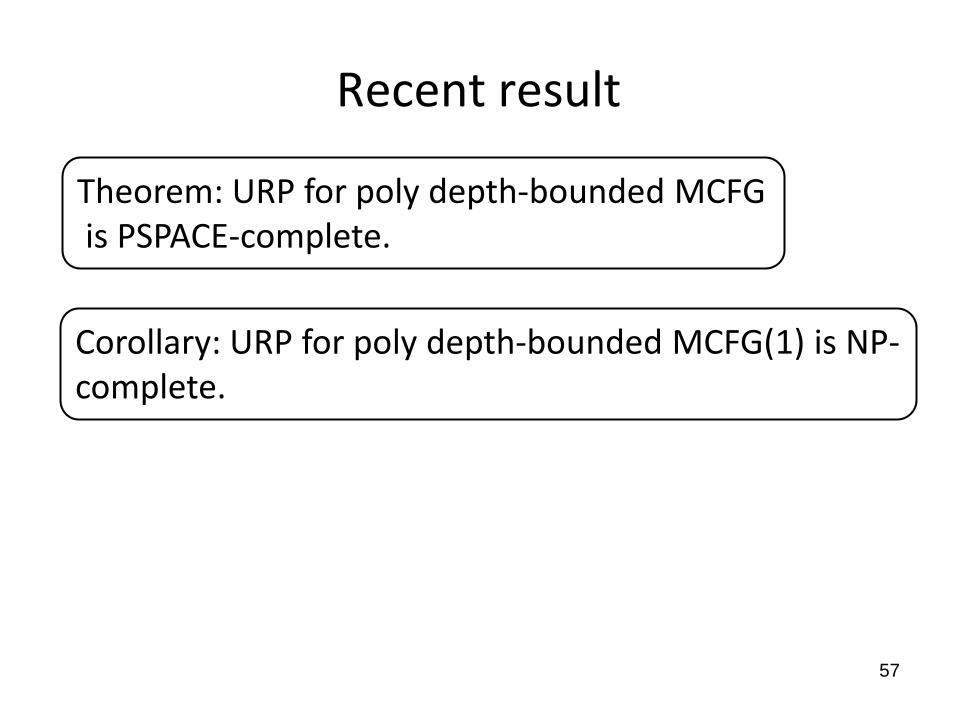
Theorem: URP for poly depth-bounded MCFG is PSPACE-complete.

Corollary: URP for poly depth-bounded MCFG(1) is NP-complete.

Summary

non-deletion

dimension depth Universal recognition

- - - DEXP-complete

required - - PSPACE-complete

- bounded - NP-complete

- - poly PSPACE-complete

- - poly, (i-1)-bounded alternation

Σi/πi-complete

- - poly, rank 1 NP-complete

58

[KNSK94]

[Seki10]

Appendix

59

60

61

• Original paper on CYK algorithm (July, 1965).

• Dr. S. Eddy, a system biologist, Washington U. asked Dr. Kasami to send a copy

(Apr. 2002).

• Dr. Kasami searched his house for a week, found one at last and sent it to Dr. Eddy.

62

noncoding RNA

• ncRNA (noncoding RNA) – RNA not translated to protein, some of them play important

roles in bio-chemical reactions (functional RNA).

DNA

ncRNA ncRNA mRNA

protein

transcription transcription

translation

gene gene gene

63

Structures of ncRNA

• Primary structure: sequence of bases A, U, C, G C U U C A U C A G A A A A U G A C (easy to obtain by next-generation sequencer) • Secondary structure: folding structure by hydrogen bonding between bases • Ternary (3D) structure

RNA secondary structure prediction

Co-relation between

structure & function

⇒ Genomic drug discovery, etc.

Problem: Given an RNA primary sequence, predict its secondary structure

64

65

Stem-loop structure

5’—C A A U G A C—3’

C•G U•A U•A

U C A A

C U U C A U C A G A A A A U G A C

nested loop

stem

66

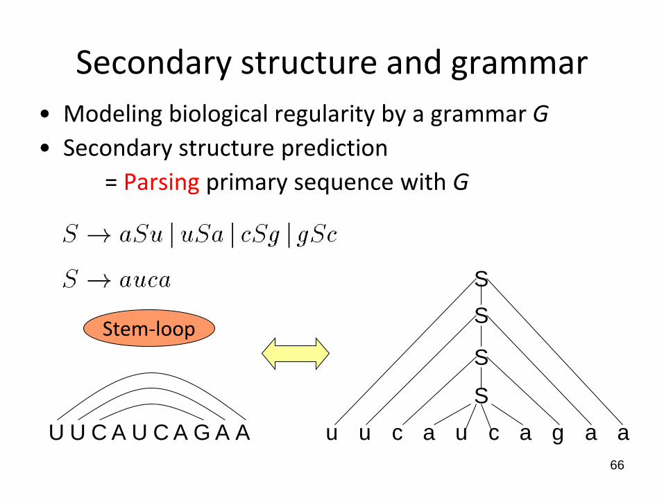
Secondary structure and grammar

• Modeling biological regularity by a grammar G • Secondary structure prediction = Parsing primary sequence with G

U U C A U C A G A A

S

S

S

S

u u c a u c a g a a

Stem-loop

67

Pseudoknot

• CFG cannot represent pseudoknot.

5’—C U U C

A A G A C U

U G A C—3’

• • • • • •

A

A

A

C U U C A U C A G A A A A U G A C

Crossed

HDV_ribozyme

• Hepatitis delta virus ribozyme

• length: 87−91

68

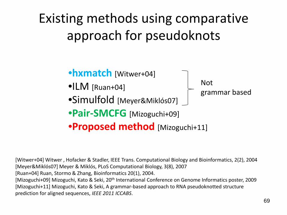
Existing methods using comparative approach for pseudoknots

69

[Witwer+04] Witwer , Hofacker & Stadler, IEEE Trans. Computational Biology and Bioinformatics, 2(2), 2004 [Meyer&Miklós07] Meyer & Miklós, PLoS Computational Biology, 3(8), 2007 [Ruan+04] Ruan, Stormo & Zhang, Bioinformatics 20(1), 2004. [Mizoguchi+09] Mizoguchi, Kato & Seki, 20th International Conference on Genome Informatics poster, 2009 [Mizoguchi+11] Mizoguchi, Kato & Seki, A grammar-based approach to RNA pseudoknotted structure prediction for aligned sequences, IEEE 2011 ICCABS.

•hxmatch [Witwer+04] •ILM [Ruan+04]

•Simulfold [Meyer&Miklós07]

•Pair-SMCFG [Mizoguchi+09] •Proposed method [Mizoguchi+11]

Not grammar based

Prediction accuracy 70

0

10

20

30

40

50

60

70

80

90

100

F-m

easu

re [%

]

Input sequeces

hxmatch Pair-SMCFG Proposed Method

Average F-measure:

hxmatch: 69.85 %

Pair-SMCFG: 64.73 %

Proposed Method: 65.26 %

Data set: 8 families from Rfam

database [Griffiths-Jones+05].

[Griffiths-Jones+05] Griffiths-Jones, Moxon, Marshall, Khanna, Eddy & Bateman, Nucleic Acids Res., 33, 2005

Thank you!

71