1

Multiple Benchmarks and Portfolio Allocation:

Why Investors do not Diversify Enough

Anna Dodonova†

Visiting Assistant Professor in Finance

Henry B. Tippie College of Business

The University of Iowa

Iowa City, IA, 52242-1000

E-mail address: anna-dodonova@uiowa.edu

† I am extremely grateful to Richard Thaler for his support and invaluable comments. I also benefited a lot from discussions with Roger Gordon, Yuri Khoroshilov, Terrance Odean, and participants of the Berkeley Summer Institute in Behavioral Economics.

2

ABSTRACT

This paper analyzes the behavior of loss-averse investors and its implications to

the portfolio choice, portfolio management, and asset pricing. The distinctive

feature of this paper is the recognition of investors’ ability to use several

benchmarks in evaluating their portfolio performances. Using the ideas of mental

accounting, the model shows that an investor who, in reality, has a number of

benchmarks to evaluate his portfolio performance will not want to completely

diversify his unsystematic risk. I show that even in the case when all investors are

identical they will not hold identical portfolios and, thus, their behavior cannot be

described by the behavior of a representative investor. A new approach developed

in this paper also helps to explain an observed time-series autocorrelation of stock

returns and the effect that a firm value and book-to-market ratio have on its

expected stock returns. Applied to the portfolio management, it implies that, in

order to maximize a client’s expected utility, a portfolio manager should follow

the contrarian strategy (buy past losers). The paper also has implications about the

design of the optimal incentive contract for the portfolio manager.

3

1. Introduction

Even though the traditional finance paradigm that assumes that agents follow axioms of

the Expected Utility Theory (Von Neumann and Morgenstern [1947]) is extremely

simple and, therefore, very appealing, this framework along does not allow one to fully

understand individual trading behavior (e.g., the fact that investors do not diversify

enough) and the puzzling behavior of stock returns (e.g., high mean and volatility and the

time series correlation of stock returns1). Difficulties faced by the traditional paradigm

gave rise to a number of behavioral theories that try to explain “the natural order of

things” by assuming some kind of irrationality in people’s behavior. Overconfidence,

prospect theory, regret aversion, and mental accounting are just several examples of

behavioral theories that help to capture many of the known patterns of individual choice

under uncertainty2. And even though it is very difficult to rank behavioral theories in

their order of importance, some of them have very well documented empirical support

and, therefore, are very difficult to ignore. This paper deals with one of these well-

documented behavioral theories: prospect theory. The main idea behind prospect theory

is that people’s utility depends not on their wealth or their consumption but rather on

their gains and losses in comparison with some reference point. Prospect theory assumes

that people are loss averse, i.e., their utility from gains is lower than their disutility from

the same losses and that they are risk-averse over gains and risk-loving over losses. It

also assumes that people tend to overestimate small probabilities and underestimate large

1 See Mehra and Prescott [1985] (high mean and volatility of stock returns); Jegadesh and Titman [1993] and Conrad and Kaul [1988, 1989] (positive short run auto correlation of stock returns); De Bond and Thaler [1985, 1987] and Fama and French [1988] (negative long-run correlation of stock returns) 2 See Hirshleifer (2001) for an excellent review of existing behavioral theories and their applications to the Finance.

4

ones. And a number of experimental evidences (see, e.g., Kahneman and Tversky (1979,

1991) and Kahneman, Knetsch and Thaler (1990)) leave no doubt that people are, indeed,

behaving as if they are loss-averse.

There are several papers (see e.g., Benartzi and Thaler [1995]; Barberis, Huang, and

Santos (1999); Barberis and Huang (2000); and Shumway (2002)) that apply ideas of

prospect theory to asset pricing.

In this paper I continue to investigate how the behavior of loss-averse investors affects

the stock market. Unlike all previous studies I am not trying to look only at the behavior

of asset prices but rather on the investment decisions of loss-averse investors and the

effects of these decisions on the investors’ portfolio allocation. The main question that I

am trying to answer is why people do not diversify enough. According to the mean-

variance frontier theory an optimal investment portfolio should be a combination only of

a risk-free asset and a market portfolio. If this is so, then how can we explain the

existence of different types of specialized mutual funds that only invest in some small

portions of the market (e.g., funds that invest only in growth firms, large cap firms, small

cap firms, etc.) in the semi-strong efficient market? Having these specialized mutual

funds means that people sometimes do not want to hold a market portfolio, i.e., they do

not want to diversify all their unsystematic risk. A new approach presented in this paper

shows that even in the world when all investors have the same preferences, none of them

wants to diversify completely and people’s investment portfolios will differ among

5

people. This, in particular, implies that there is no representative investor even when all

investors are identical.

The fact that an investor’s utility depends on his gains and losses has a very important

implication to the portfolio management. Currently every portfolio manager has a

benchmark that he either tries to follow (as in the case of passive portfolio management)

or to beat (in the case of active portfolio management). So, when a client hires a portfolio

manager or invests his money into some mutual fund, he must choose the benchmark that

is appropriate for him.

How can the investor choose the unique benchmark? Is it possible for the investor to just

ignore bits of information that are available on the market and focus only on the

performance of his portfolio and the unique benchmark he uses? How a sophisticated

investor who knows the benefits of diversification and invests in S&P 500 (which more

or less tracks the market return) can resist the temptation to compare his return with

NASDAQ? The problem of benchmark choice is even more severe for ordinary investors

whose benchmarks are often influenced by different news sources (TV, Wall Street

Journal, friends, internet sites, etc.) So, it seems natural to assume that when a person

evaluates his portfolio performance he compares his return with the returns on each of his

several benchmarks (e.g., most popular market indices, some popular stock that is in the

news, portfolio of his sister, etc.) separately and his utility somehow depends on these

comparisons3. Thus, as soon as a person observes a return on one of his benchmarks he

3 An alternative assumption could be that a person constructs some “weighted average” benchmark (out of all his possible benchmarks) and then compares its return with the return on his portfolio. However, it is

6

immediately compares it with his portfolio return and feels joy or disappointment

depending on how favorable this comparison is. If later on he gets news about the

performance of any other benchmark he uses, he makes his comparisons once again.

Every one of these comparisons is assigned to its own specific mental account (Thaler

[1985], [1990], [1999]). Mental accounts are evaluated with some frequency (Read,

Loewenstein, and Rabin [1998]). The person gets utility/disutility from every account

evaluation and uses them as the components of his aggregate utility function.

However, when the client with several different benchmarks on his mind comes to the

portfolio manager and says “I would like to have a return that is close to the return on the

high-tech companies but at the same time I do not want to have significant losses in

comparison with the average market return”, the natural response of the portfolio

manager is “You need to choose which one would you like me to follow. I cannot track

two indices simultaneously”. And the investor has to choose one of the benchmarks (or,

at best, a linear combination of them). So, the real problem is not that clients don’t know

what do they want but that portfolio managers don’t know how to deliver to them what

they want.

In this paper I provide a recommendation of how to deal with loss-averse investors who

want to use several benchmarks to evaluate their portfolio performance. I show that, in

order to maximize clients’ expected utility, the portfolio manager should not diversify

completely and should follow a contrarian strategy (invest in past losers). If we want to

hard to imagine that a person first gathers information about returns on his benchmarks, then calculates the “weighted average” return and only after that makes his comparison.

7

make a simple incentive contract for a portfolio manager then we should force him to use

a benchmark that is a non-linear function of the benchmarks proposed by a client and is

biased toward the worst performing one (i.e., if the client uses portfolios A and B as his

benchmarks, the manager should try to invest so that the return will be close to min{rA,

rB}+some fixed premium).

This paper also shows that investors’ choice of the benchmarks may help to explain the

home-bias effect and the existing predictability (positive short-run and negative long-run

correlation) of stock returns. Investors’ choice of benchmarks may also explain why firm

value and the market/book ratio affect the expected return, why initial underpricing of

IPOs will partially disappear in several months of trading and why during the IPO waves

the IPO underpricing is not so severe.

The original version of prospect theory does not specify how people form their

benchmarks. In experimental studies it is assumed that people consider their current

wealth as their benchmark and an increase in their wealth is treated as a gain while a

decrease is treated as a loss. This assumption was used by Barberis, Huang, and Santos

(1999), and Barberis and Huang (2000) (who constructed the model of asset price

behavior that explains high risk premium and negative autocorrelation of returns) and by

Shumway (2002) (who shows that in the market populated by loss-averse investors the

pricing kernel is not a monotone function of the market return and that investors value the

upside and downside risks differently).

8

The stock market, however, provides a number of other possible benchmarks for an

investor. For example, an investor may compare his portfolio return with the risk-free

rate of return4. He also may compare his return with the market rate of return. It is natural

to feel a gain if you overperformed the market and a loss if you underperformed it. An

investor who gets his information from watching CNN, reading his mutual fund reports,

and, occasionally, reading the Wall Street Journal or surfing investment-related sites on

the internet, may compare his return with returns on different market indices, with returns

on most known large companies, or with returns on the “hot” companies that are in the

news. Dodonova (2002) proposes that people may have regrets when they see that some

asset performs well but they did not invest much in it, i.e., the benchmark that investors

use when they evaluate their portfolio performance is not fixed ex ante but rather depends

on the ex post stock performance.

In this paper I make another step in the recognizing investors’ right to have different

benchmarks. Using the idea of mental accounting proposed by Thaler (1985, 1990, 1999),

I assume that investors may simultaneously use several benchmarks to evaluate their

portfolio performance. Namely, an investor separately compares his portfolio returns with

each of his benchmarks and his utility depends on each of these comparisons.

The main intuition behind my model is the following. At the time when the initial

investment is made investors do not expect to outperform all of their benchmarks. Since

investors are risk-loving over losses and since their disutility from the losses is higher

4 Barberis, Huang, and Santos (1999), Barberis and Huang (2000), and Shumway (2002) argue that their results will not change if investors use risk-free rate as a benchmark.

9

than their utility from the same gains, investors want to have some risk exposure, so that,

they would be able to gamble over the losses relative to their benchmarks. Thus, investors

do not diversify enough. In the symmetric world when all investors and all assets are the

same, the exogenous supply of assets will lead to the situation in which identical

investors will allocate their portfolios differently. In the dynamic setting investors’ desire

to fix their relative gains and to gamble over their relative losses makes them more

willing to reallocate their portfolios toward the assets that their portfolios currently

overperform (i.e., toward the past losers). Such portfolio reallocation will lead to the

market underreaction on bad/good news and to the positive autocorrelation of stock

returns. So, when investors delegate their investment decisions to the portfolio manager

or put their money into a mutual fund, they want a portfolio manager to be biased toward

the worst performing asset, so that they will have a fixed gain over one of their

benchmarks and a gamble over the other.

The rest of the paper is organized as following. In part two I develop a basic 2-period

model of investors’ behavior, prove the existence of the equilibrium and analyze its basic

properties. In part three I discuss some of the empirical implications of the basic model.

In particular, I prove that investors never want to diversify all unsystematic risk and that

this economy does not have a representative investor even if all investors are identical. In

part four I generalize the basic model to a 3-period case and discuss its application to a

portfolio management. In part five I conclude.

10

2. Basic Model

In this part of the paper I construct a basic 2-period model of investors’ behavior based

on the assumption that investors care not only about their final wealth but also about their

gains and losses relative to some benchmarks. The classic version of the prospect theory

(Kahneman and Tversky [1979, 1991]) assumes that investors care about changes in their

wealth. They are risk-averse over gains and risk-loving over losses and their utility from

gains is lower than their disutility from the same amount of losses. Kahneman and

Tversky (1992) proposed the following individual’s utility function:

( )

<−−≥=

0,0,)(

xxxxxv α

α

λ (1)

where x is the change in person’s wealth, 10 <<α and 1>λ are some parameters. Based

on the experimental data, Kahneman and Tversky (1992) estimate 88.0=α and

25.2=λ .

Even though a number of evidences confirm the loss-aversion assumption, it is still

unclear how people chose their benchmarks. Prospect theory assumes that people care

only about their gains and losses (i.e., their past wealth serves as their benchmarks) and

Barberis, Huang, and Santos (1999), Barberis and Huang (2000) and Shumway (2002)

use this assumption in their asset pricing models. There are, however, evidences that

people’s reference point may be influenced by aspiration, expectations, norms and social

11

comparisons (see, e.g., Easterlin (1974), van Praag (1971), and van de Stadt, Kapteyn,

and van de Geer (1985))

The existing financial markets provide a wide range of possible benchmarks. Generally

speaking, an investor may compare his return with a return on any investment

opportunity that he considered in the past but decided not to pursue. Investment in T-bills

or T-bonds, which guarantees a risk-free rate of return, is one of these opportunities. A

more sophisticated investor, who is familiar with the concept of diversification, will be

interested in how his portfolio performed in comparison with the market rate of return

(this idea was used by Abel (1990) who assumes that a person’s utility depends on the

difference between his consumption and the aggregate consumption level in the

economy). A regret-averse investor who feels regret every time his assets turn out not to

be on the top of the market, compares his portfolio performance with the maximum

payoff he could have had if he, ex ante, invested in the best ex post portfolio (see

Dodonova [2002]).

Many times, however, it is hard for an investor to decide up-front which benchmark he

will use next year when he evaluates his portfolio performance. Consider, for example, an

investor who decides whether to invest in the high-tech industry (NASDAQ index) or in

more traditional businesses (Dow Jones). For simplicity, let us ignore the difference in

risks by assuming that investors adjust their risk exposure by investing in the money

market account. Next year, when he will get his mutual fund report, he may easily

12

compare his return with returns on NASDAQ and Dow Jones indices and, depending on

which index he chooses as a benchmark, he may feel gain or loss.

Applying ideas of mental accounting (Thaler [1985], [1990], [1999]) one may argue that

nobody prevents the investor from comparing his return with both returns: on NASDAQ

and on the DJ. Thus, the investor’s utility must be some average of his utility from the

comparison of his return with the return on NASDAQ and his utility from the comparison

with the DJ, and not the utility from the comparison of his return with the average returns

on NASDAQ and DJ. So, an investor may use several different benchmarks

simultaneously.

In this paper I assume that investors care about both: their wealth and their financial gains

and losses, i.e. I assume that their utility function is given by

( ) ( ) ( )pRvwuU δδ +−= 1

where w is the investor’s wealth and Rp is his portfolio return.

I assume that an investor’s utility out of his wealth )(wu is an increasing and concave

function and, to prevent the possibility of negative wealth, I assume that −∞=)(wu for

w<0. Function )( pRv represents the investor’s utility from his portfolio performance and

depends on the benchmarks that the investor uses to evaluate his portfolio return.

13

Following Kahneman and Tversky (1992) and allowing investors to have different

benchmarks, I assume that the investor’s utility from comparing his portfolio with

benchmark i is

( )( )

<−−−≥−−

=−0,0,

)(ippi

ipipipi RRRR

RRRRRRv α

α

λ (2)

and the total utility that he gets from comparing his portfolio return with different

benchmarks is given by:

( ) ( )∑=i

piip RvqRv (3)

where 1=∑i

iq and 0≥iq .

Assume that there are 2 assets in the economy: asset #1 and asset #2 (these assets may be

viewed as industry-specific indices) and that investors use these assets as their benchmark

portfolios. Assume there is a continuum of investors (numbered by c ) on the market with

the total wealth normalized to 2.

In the basic framework of the model I consider a 2-period case. At t=0 investors make

their investment decisions and invest cγ portion of their wealth in asset #1 and )1( cγ−

in asset #2, where cγ may be different for different investors. At t=1 both assets are

liquidated and investors consume the proceedings. The liquidation values of assets #1 and

14

#2 are 1R and 2R and, to make things simple, I assume that 1R and 2R are independent

and identically distributed on ( )∞,0 random variables.

Thus, the problem of an investor with an initial wealth of $1 is to maximize

( )

−−+

−+−≡

2

2

1

1 )1()1()(maxpR

REvqpR

REvqREuU pcpccpccc

δδγγ

(4)

s.t.:

22

11

1R

pR

pR cc

pγγ −

+= (5)

where 1p and 2p are the prices for the 1st and 2nd assets at t=0.

In general, I assume that the parameters of the utility function cδ (which measures how

important gains and losses are for the investor) and cq (which measures the relative

importance of the first asset as the benchmark) may be different for different investors,

but I will concentrate on the case in which they are equal, i.e., all investors have the same

preferences.

The equilibrium conditions for the stock market are given by

∫ =C

c pdc 1γ (6)

15

and

∫ =−C

c pdc 2)1( γ (7)

where C is the set of investors.

Using the assumption that the total number of investors is 2, i.e., that 2=∫C

dc , we can

find

221 =+ pp (8)

and may use (8) instead of (7) in an equilibrium analysis.

The maximization problem (4) and (5) together with the market clearing conditions (6)

and (8) determine the equilibrium in the economy.

Before analyzing the properties of the equilibrium portfolio allocations and asset prices,

we need to check that the equilibrium, described by (4), (5), (6) and (8), exists. The

following theorem proves the existence of the equilibrium and describes the basic

properties of the equilibrium investment allocation.

Theorem 1

1) (Existence)

16

There is an equilibrium portfolio allocation cγ and asset prices 1p and 2p that satisfy

(4), (5), (6) and (8). Moreover in any equilibrium [ ]1,0∈cγ

2) (Local monotonicity)

If )( 1pcγ is the solution to the investor’s problem (4) subject to (5) and (8), then

0)(

1

1 <dp

pd cγ at any point where )( 1pcγ is continuous and differentiable function of 1p

3) (Global monotonicity)

If 2/1≥cq , 11 ≤p , and at least one of these inequalities is strict, then in any equilibrium

2/1>cγ .

Proof: see appendix

The intuition behind the results of Theorem 1 is simple: an increase in the first asset price

1p (and, thus, a corresponding decrease in 2p ) makes investment in the first asset less

attractive, and, thus, decreases equilibrium cγ . When the investor is more concern about

his portfolio performance relative to the first benchmark ( 2/1>cq ) or when the expected

return on the first asset is higher than on the second ( 11 <p ), the investor wants to hold

more of the first asset, i.e., 2/1>cγ .

3. Empirical Implications

17

To understand how loss-aversion affects investors’ behavior and asset prices, let us

assume that all investors are the same, i.e., that δδ =c and qqc = for c∀ . Moreover,

assume that investors do not have any preferences towards any particular asset and that

they value their gains and losses relative to the first asset in the same way as their gains

and losses relative to the second one, i.e., assume that 2/1=q . Thus, the investor’s

maximization problem becomes:

( )

−+

−+−≡

2

2

1

1

2)1()(max

pR

REvpR

REvREuU pppcc

δδγγ

(9)

s.t.

22

11

1R

pR

pR cc

pγγ −

+= (10)

Together with equilibrium conditions (6) and (8), investor’s problem (9) and (10)

determines an equilibrium in the economy. Note that, although )(xu is a concave

function, )(xv is concave for x>0 and convex for x<0. Thus, we cannot claim that the

solution to the investor’s problem (9) and (10) is unique, and, as I will show in

Proposition 1, investors do choose different portfolio allocations.

To get the intuition on how the equilibrium looks, note, that since investors treat both

assets in the same way, we may expect to have 121 == pp . Given that prices on both

assets are equal, there are two forces that affect an investor’s decision. First, his risk-

aversion over his final wealth (concavity of )(xu ), leads to the desire to diversify and to

18

choose 2/1=cγ . Second, his loss-aversion together with his risk-loving over losses

makes him willing to gamble and, thus, unwilling to diversify. If the investor is

sufficiently loss-averse (δ is sufficiently large) than his desire to gamble may outweight

his desire to diversify and his optimal portfolio allocation cγ will be different from the

complete diversification ( 2/1≠cγ ). (In all that follows I assume that δ is sufficiently

large to make the loss-aversion effect important.) Because the investor treats both assets

in the same way, he is indifferent between the following two portfolios: 21 )1( RR γγ −+

and 21)1( RR γγ +− . Thus, to allow the stock market to clear, ½ of investors will invest γ

in asset #1 and )1( γ− in asset #2 while the remaining ½ of investors will invest )1( γ−

in asset #1 and γ in asset #2.

Figure 1 presents the investor’s expected utility function )(γU as a function of his

investment in the first asset.5 As it can be seen in this figure, )(γU has an M-shape: a

perfect diversification ( )2/1=γ is a local minimum of the expected utility function while

15.0=γ and 85.0=γ are two symmetric global maximums. Thus, in the equilibrium

nobody will perfectly diversify; ½ of the investors will invest 15% of their wealth in asset

#1 and 85% in asset #2 while the remaining ½ of the investors will invest 85% in asset #1

and 15% in asset #2. So, the total investment in both assets are the same.

The following proposition summarizes the discussion above.

5 For the expositional purposes I choose xxu ln4.0)( += , 88.0=α , 25.2=λ , 945.0=δ , and

{ }9.1,1.0=iR with equal probabilities.

19

Proposition 1.

If all investors are the same ( δδ =c and qqc = ), and treat all assets in the same way

(q=1/2), then

1) In any equilibrium asset prices must be the same 121 == pp .

2) Nobody will diversify completely ( 2/1≠cγ ).

3) If some investors invest γ in asset #1 and )1( γ− in asset #2, then an equal number

of investors will invest )1( γ− in asset #1 and γ in asset #2.

Proof: see appendix.

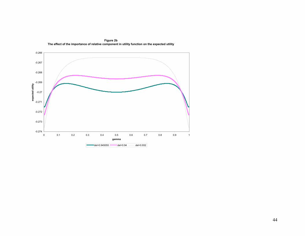
As the discussion above indicates, the desire to diversify depends on how important the

“relative” component of the utility function is. Figures 2a and 2b present the expected

utility function )(γU for different values of δ . When δ increases, the relative part of

the utility function becomes increasingly important (Figure 2a). The maximums of the

expected utility function moves toward complete specialization and complete

diversification becomes more and more painful. If δ becomes too large, an M-shape of

the expected utility function transforms into a U-shape and complete specialization

becomes an optimal portfolio allocation. When δ decreases (Figure 2b), the “absolute”

part of the utility function becomes more important and the optimal portfolio allocation

moves toward perfect diversification. When δ becomes too small, an M-shape of the

expected utility function transforms into an arch-shape.

20

Another important implication of the basic model may be received if we look at how

investment decisions depend on the volatility of assets returns. Standard asset-pricing

models with risk-averse investors predict that higher volatility makes the benefits of

diversification even higher and, thus, investors should diversify more in the more volatile

markets. If, however, investors are loss averse, then high volatility increases the possible

relative losses and makes an investor, who is risk-loving over losses, gamble more. Thus,

there are two different forces that affect investors’ decisions to diversify and higher risk

may increase or decrease this desire to diversify.

Now, let us relax the assumption that people treat all assets in the same way and, instead,

assume that people care about their portfolio performances relative to the first benchmark

more than relative to the second, i.e., assume that 2/1>q . Since people are loss-averse,

they will try to minimize their losses in comparison with the first benchmark. Thus, all

else equal, they will buy more of the first asset. Since the supply of assets is exogenous,

this behavior will lead to an excess demand on asset #1 and an excess supply of asset #2.

Thus, in the equilibrium prices should adjust so that 21 pp > and, as a result, the

expected return on the first asset must be lower than the return on the second

<

2

2

1

1

pR

EpR

E . Figure 3 presents how the expected utility function depends on the

first asset’s price6. When the first asset becomes more expensive, it becomes less

attractive for the investors. The M-shape of the expected utility function becomes

asymmetric: the left local maximum becomes more attractive and it moves to the left

6 An increase in the importance of the first asset in the “relative” component of utility function (i.e., an increase in q) has an opposite effect

21

(more investment in second asset) while the right local maximum becomes less attractive.

And only the left local maximum will be the global maximum when 21 pp > and q=1/2.

An increase in q will have the opposite effect. Thus, if q>1/2 we should have 21 pp < in

order to have two local maximums such that 2,1, 2/1 cc γγ << . Note, that the optimal

portfolio allocation cγ is not a continuous function of 1p or q (Figure 4). For example,

when q=1, 21 pp < , the optimal solution 15.0<cγ while at 21 pp > we have 85.0>cγ .

This is so because at 21 pp = we have a symmetric M-shape expected utility with two

global maximums 15.0=cγ and 85.0=cγ . When 1p increases from 21 pp < to

21 pp > , the global maximum jumps from the left local maximum to the right local

maximum.

The following proposition summarizes the discussion above.

Proposition 2

If all investors are the same ( δδ =c and qqc = ) and care about their portfolio

performance relative to the first asset more than relative to the second asset (q>1/2), then

in the equilibrium asset #1 must be overpriced )1( 21 pp >> and must have a lower

expected return than asset #2

<

2

2

1

1

pR

EpR

E .

Proof: see appendix.

22

Proposition 2 may have a number of empirical implications if we will understand how

investors form their benchmarks. For example, if they use market indices as benchmarks,

an inclusion of some stock in a market index will result in an abnormal positive return

and in lower future expected returns. If people more often compare their portfolio

performance with the performance of large firms than with the performance of small

firms then the firm market value should negatively affect the expected stock returns7. If

people pay more attention to the stocks that performed well in the past, then high past

return will increase the importance of these stocks in the relative component of the

investor’s utility function, and, thus, will lead to higher demand and higher (than

“fundamental”) equilibrium price on this stock. So, we should observe a market

overreaction and the negative long-run correlation of stock returns. Finally, if we are in

the situation of a stock market bubble and people pay attention to “hot” stocks that are in

the news (like amazon.com), then those stocks must also have abnormal returns and low

future expected returns. For example, if a high market-to-book ratio makes a firm “hot”

and draws an additional attention, then we should expect the market-to-book ratio to have

a negative effect on the firm’s expected returns8. Similarly, since any IPO draws

investors’ attention, we should expect abnormal returns on IPOs and we should expect

this return to partially disappear over time. Furthermore, one may argue that during stock

market booms or during stock bubbles a person will pay more attention to the stock

market and his benchmark returns will be more distinctive than when the stock market is

stable. So, the model described in this paper may have more power during stock market

booms or bubbles. Moreover, this model may also explain the existence of stock bubbles:

7 This result is consistent with Fama and French (1993). 8 This result is also consistent with Fama and French (1993).

23

when some industry shows an abnormal return, investors start to compare their returns

with the return on this industry, and, thus, they will invest more into this industry which,

in turn, will lead to even higher stock prices.

Different people may have different utility functions, and, in particular, different

benchmarks to which they want to compare their returns. For example, people more often

compare their portfolio returns with home stock returns or with stock returns of firms

they work for. However, if different people have different benchmarks ( cq are different

among people) but, on average, all assets look the same ( )

=∫ 2/12/1

Cc dcq , we should

not expect to have any effect on the stock prices. We should, however, expect people to

invest more in their home country stock market (home-bias effect) or in the company

they work for. The following proposition summarizes the discussion above.

Proposition 3

If, for any [ ]1,0∈q , the number of investors with preferences q is the same as the number

of investors with preferences (1-q), then loss-aversion has no effect on stock prices

( 121 == pp ), but people, who care more about their portfolio performance relative to the

first asset than they do relative to the second one ( 2/1>cq ), invest more in the first asset

( 2/1>cγ ) while people who care more about their portfolio performance relative to the

second asset ( 2/1<cq ), invest more in the second asset ( 2/1<cγ ).

Proof: This result directly follows from Theorem 1.

24

4. Portfolio Management

In the basic set up of the model analyzed in parts 2 and 3, I assumed that investors do not

change their portfolio allocations during the whole period of investment (say, a year). If,

however, investors delegate their portfolio allocation decisions to a portfolio manager,

how would they like the manager to manage their portfolios? To get the intuition, assume

that at t=0 the manager invests γ in asset #1 and )1( γ− in asset #2 and sometime during

the year (at t=1/2) he sees that asset #1 is outperforming asset #2. Since there is a high

probability that asset #1 will overperform asset #2 over the year, investors’ returns most

likely will be higher than the return on asset #2 and lower that the return on asset #1.

Since people are risk averse over gains and risk-loving over losses, they want to fix their

relative gains relative to asset #2 and to gamble over losses relative to asset #1. Thus,

investors would want their portfolio manager to reallocate their portfolios toward asset #2

(past loser). In order to make the manager buy more of the past loser, investors need him

to be biased toward the minimum return, i.e., they want the manager to use a benchmark

that is close to the drr +},min{ 21 , where ir is the return on investors’ benchmarks and

d>0 is some positive premium. Moreover, such reallocation during the year will result in

the market underreaction and will lead to the positive short-run correlation of returns.

To see that this intuition works, let us generalize the basic 2-period model described in

part 2 to a 3-period model in which (1) at t=0 investors delegate their investment

decisions to the portfolio manager; (2) at t=1/2 the portfolio manager reallocates his

25

clients’ portfolios based on the information released at that time; and (3) at t=1 all assets

are liquidated, investors evaluate their portfolio performances and consume the

proceedings. Assume that the portfolio manager represents the interests of his clients and

wants to maximize their expected utility.

As in the basic 2-period model of part 3, assume that there are 2 securities that at t=1 will

pay 1R and 2R respectively. Assume that at time { }1,2/1∈t news ti,ξ about each asset

{ }2,1∈i is realized, and the final realized payoff is equal to 1,2/1,1 iiiR ξξ ++= . The

signals about assets’ final returns are independent across time, i.e., ( )1,21,1 ,ξξ is

independent on ( )2/1,22/1,1 ,ξξ . For tractability, assume that ti,ξ is equal to D or D− with

equal probabilities (where D<1/2) and that t,1ξ and t,2ξ are perfectly negatively

correlated. The latter assumption is needed only to simplify calculations: it allows us to

reduce the number of states of the world. To make things even more simple, assume that

at t=0 the portfolio manager does not take into account the fact that people’s utility

depends on the relative return on their portfolios, and he diversifies all the unsystematic

risk, i.e. he invests equally into assets #1 and #2.9

9 As was shown in the part 3 of the paper, an optimal portfolio allocation at t=0 should include an unequal amount of first and second assets and, thus, not all of unsystematic risk should be diversify. The model described here, however, do not allow one to solve analytically for an optimal portfolio allocation at t=0. To make things simple, I assume that at t=0 portfolio manager invests equally in both assets, but the intuition behind theorem 2 should work for any initial investment allocation.

26

The investors’ utility function is given by ( ) ( ) ( )pRvwuU δδ +−= 1 , where ( )pRv is

given by (3).10 Given that at t=0 the portfolio manager invests equally in assets #1 and

#2, at t=1/2 he wants to maximize the expected shareholder’s utility U , i.e. he wants to

solve the shareholder’s problem (4)-(5) given the information available at time t=1/2

( 2/1,1ξ and )2/1.2ξ . Assume that this portfolio manager is operating in an environment

where all other investors want to maximize their “absolute” expected utility ( )wu , i.e.,

they perfectly diversify. The following theorem shows that, in order to maximize their

clients’ expected utility, a portfolio manager should follow a contrarian strategy and

invest in past losers

Theorem 2

Assume that at t=1/2 asset #1 outperforms asset #2, i.e. assume that at t=1/2 we have

D=2/1,1ξ and D−=2/1.2ξ . Given that asset prices are formed by investors who

maximize their “absolute” expected utility ( )wu (and, thus, perfectly diversify), a

portfolio manager who wants to maximize his clients’ utility ( ) ( ) ( )pRvwuU δδ +−= 1

should reallocate his portfolio toward asset #2.

Proof: see appendix.

10 Here I assume that investors evaluate their portfolio performance only at the end of the year and compare their annual return with the annual return on each of the assets.

27

In the case when asset prices are formed by the people who want to diversify all of their

unsystematic risk, it is easy to show that the price on asset i at time t=1/2 will be11

2/1,1 iip ξ+= . Thus, an expected return between t=1/2 and t=1 will not depend on the

return between t=0 and t=1/2 and will be zero for both assets. If, however, portfolio

managers who maximize their clients’ expected utility ( ) ( ) ( )pRvwuU δδ +−= 1 affect

the price formation, they impose an excess demand on the past loser and will make the

price on the first asset (that performed good at t=1/2) to be below 2/1,11 ξ+=ip and the

price on the second asset (that performed poorly at t=1/2) to be above 2/1,11 ξ+=ip .

Thus, we should expect to have a positive return on past losers and a negative return on

past winners, i.e., we should expect a negative correlation of stock returns.

5. Conclusion

This paper presents a model of the behavior of loss-averse investors. Based on the ideas

of prospect theory (Kahneman and Tversky [1979], [1991]) and mental accounting

(Thaler [1985], [1990], [1999]), I assume that investors care not only about their final

wealth but also about their relative return in comparison with a number of different

benchmarks. Since the stock market provides investors a number of possible benchmarks,

I assume that investors’ utility depends on their gains and losses relative to every

benchmark they use.

11 See Dodonova (2002) who uses the similar setup and shows that the “rational” prices must be equal to the expected future payoff.

28

The model presented in this paper shows that even if investors are identical and do not

have any ex ante preferences toward any one particular benchmark, they will hold

different portfolios and none of them will diversify all of his unsystematic risk. The way

in which investors form their benchmark portfolios may explain a number of observed

anomalities in investors and stock price behavior, such as the predictability of stock

returns, the home-bias effect in investors’ portfolio allocation, and the fact that employee

invest an abnormal portion of their wealth into their own company stocks.

The model has an important implication that deals with portfolio management. It

proposes that portfolio managers should recognize investors’ desire to have several

benchmarks simultaneously: the benchmark that managers should follow must be biased

toward the minimum among the investors’ benchmarks’ returns, and, all else being equal,

should follow a contrarian strategy (buy past losers).

29

Appendix.

Proof of theorem 1

(1) Existence

By substituting (5) and (8) into (4), we can rewrite (4) as

( )

( ) ( )

−

−−+

−−

−−

+

−

−+−≡

1

2

1

1

1

2

1

1

1

2

1

1

1)1(

111

11

)1()(

max

pR

pR

Evqp

Rp

REvq

pR

pR

EuU

ccc

cccc

cccc

c γγγγδ

γγδγ

γ (A1)

Since ( ) −∞=pRu for 0<pR , any cγ that maximizes (A1) must satisfy

( )0

11

1

2

1

1 >−

−+

pR

pR cc γγ

for any 0, 21 >RR . Thus, [ ]1,0∈cγ . Since ( )cU γ is continuous

function of cγ and [ ]1,0∈cγ , equation (A1) has at leas one solution.

Denote the set of solutions to (A1) by ( )1* pγ . To complete the proof we need to show

that 11 : pdcpC

c =∃ ∫γ for some ( )1* pc γγ ∈ .

Denote

1

2

1

1

1 pR

pR

z−

−= (A2)

Using (2) and (A2), we can rewrite (A1) as

30

( )

( ) ( ) ( )( )

−+−−

+

−

−+−≡

zEvqzEvq

pR

pR

EuU

ccccc

cccc

cαα

γ

γγδ

γγδγ

)1(1

11

)1()(max 1

2

1

1

(A3)

Note that if 01 →p then ∞→z almost surely. Thus, for small enough 1p , ( ) 0>zEv

and ( ) 0<− zEv . Therefore, if 1p is small enough, then

( ) ( ) ( )( )0

)1(1>

∂−+−−∂

c

cccc zEvqzEvqγ

γγ αα

(A4)

Moreover, since u(.) is a concave increasing function, then in the case when one of the

assets’ price goes to zero, a person who maximizes ( )pREu will invest more into this

asset. In other words, [ ]1,0∈cγ P∃ such that for Pp <∀ 1 we have

( )

01

1

1

2

1

1

>∂

−

−+∂

c

cc

pR

pR

Eu

γ

γγ

(A5)

Combining (A4) and (A5) we have

( ) { }1lim 1*

01

=→

pp

γ (A6)

Similarly, one can show that

( ) { }0lim 1*

21

=→

pp

γ (A7)

Since ( )cU γ is continuous function of cγ and 1p , ( )1pµ∃ such that ( )⋅µ is continuous

and 1p∀ [ ]1,0∈∃ η such that ( ) ηγηγµ 2,1,1 ccp += , where ( )1*

2,1, , pcc γγγ ∈ . Note that if

31

( )1*

2,1, , pcc γγγ ∈ then ( )1pµ is a possible aggregate share of investment in asset 1, i.e.,

( ) ∫=C

c dcp γµ 1 for some ( )1* pc γγ ∈ . Using (A6) and (A7) we may claim that

( ) 2lim 101

=→

pp

µ and ( ) 0lim 121

=→

pp

µ . And, since ( )⋅µ is continuous there is 1p such that

1pdcC

c =∫γ where cγ is solution to (4) given (5) and (8). Q.E.D.

(2) Local monotonicity

Assume 11 ≤p (in the case when 11 ≥p the proof is the same)

( ) ( ) ( )( ) ( ) ( ) ( )( )zEvqzEvqzEvqzEvqV

ccccc

cccc 11 )1(1)1(1 −− −+−−−=

∂−+−−≡∂ αα

αα

γγαγ

γγ

Since 11 ≤p we have ( ) 0<− zEv . Since z is a decreasing function of 1p , and ( )zv is an

increasing function of z , we have ( ) ( ) ( )( )0

)1(1

1

2

<∂∂

−+−−∂p

zEvqzEvq

c

cccc

γγγ αα

.

Moreover, since u(.) is a concave increasing function, a person who maximizes ( )pREu

will invest more into an asset which price drops, i.e.,

( )

01

1

1

1

2

1

12

<∂∂

−

−+∂

pp

RpR

Eu

c

cc

γ

γγ

.

Therefore, ( )

01

2

<∂∂

∂p

U

c

c

γγ

. Moreover, if cγ is a solution to (A1), then ( )

02

2

<∂

∂

c

cUγ

γ at

cc γγ = . Thus, at cc γγ = we have

( )

( ) 0

2

21

2

1

<

∂∂

∂∂∂

−=

c

c

c

c

c

Up

U

dpd

γγ

γγ

γ. Q.E.D.

32

(3) Global monotonicity

A person wants to maximize his expected utility

( ) ( ) ( ) ( )( )zEvqzEvqp

RpR

EuU ccccccc

ccαα γγδγγδγ )1(1

11

)1()(1

2

1

1 −+−−+

−

−+−≡

Let us assume that 2/1≥cq and 11 ≤p , and at least one of this inequalities is strict. By

contradiction, assume that a solution to (A1) satisfy 2/1<cγ . Since 11 ≤p , we have

( ) ( )

−

+−

≤

−

−+

1

2

1

1

1

2

1

1

11

11

pR

pR

Eup

RpR

Eu cccc γγγγ.

Moreover, ( ) ( )zEvzEv ≤− , and, this inequality must be strict when 2/1=cq (because in

this case we must have 11 <p ) Thus,

( ) ( ) ( )( ) ( ) ( ) ( )( )zEvqzEvqzEvqzEvq ccccccccαααα γγγγ −−+−<−+−− 1)1()1(1

So, we have that ( ) ( )cc UU γγ −< 1 which contradict to the assumption that cγ is a

solution to (A1). Thus, it must be the case that 2/1≥cγ .

To complete the proof we need to show that 2/1≠cγ .

33

To do it, it is enough to show that ( )

0>∂

∂

c

cUγγ

at 2/1=cγ . And this is so because

( )

−

−+

1

2

1

1

11

pR

pR

Eu cc γγ has a unique maximum 2/1≥cγ and because

( ) ( ) ( )( ) ( ) ( )( ) .02/)1(2/)1(1

>−+−−=∂

−+−−∂zEvqzEvq

zEvqzEvqccc

c

cccc ααα

γαγ

γγ

The later is follows from the fact that ( ) 0<− zEv and ( ) ( )zEvzEv ≤− where the last

inequality is strict when 2/1=cq (because in this case we must have 11 <p ). Q.E.D.

Proof of proposition 1:

If 11 <p then, by theorem 1, any solution to (A1) must satisfy 2/1>cγ . Therefore,

∫ >>C

c pdc 11γ , i.e., condition (6) is violated. Thus, we must have 11 ≥p . Similarly, we

must have 12 ≥p , which means that 121 == pp .

To show that 2/1=cγ cannot be a solution to (A1), let us find

( )

( )( ) ( ) ( ) ( )

+−

−−+=

∂−+∂

−=

==∂

∂

−−

zEvzEvRREu

U

ccc

ccc

cc

c

1121

21

211

212/1

1)1(

2/1)(

αα

αδγγ

γγδ

γγγ

Since at 121 == pp we have ( ) ( )zEvzEv −= , and since

( )( ) ( ) 02/11 21 ==

∂−+∂

cc

cc RREu γγ

γγ

we can find

34

( ) 02/1)(

==∂

∂c

c

cU γγγ

(A8)

However,

( )

( )( ) ( )

( ) ( ) ( )

( )( ) ( ) ( ) ( )zEvRREu

zEvzEv

RREu

U

ccc

ccc

c

cc

ccc

cc

c

2

221

2

22

221

2

2

2

2112/1

1)1

21

211

211

2/11

)1(

2/1)(

−

−−

−+=

∂−+∂

−=

=

+−

−−+

+=∂

−+∂−=

==∂

∂

α

αα

ααδγγ

γγδ

ααδ

γγ

γγδ

γγ

γ

Since ( ) 0<zEv , we have that ( ) ( ) 0211

2

>

−

−

zEvc

α

ααδ . Thus, if cδ is large enough

we have that ( ) 02/1)(

2

2

>=∂

∂c

c

cU γγ

γ which means that 2/1=cγ is a local minimum of

)( cU γ and cannot be a solution to (A1).

Since in the equilibrium we must have ∫ =C

c dc 1γ , in the case when some investors invest

γ in asset #1 and )1( γ− in asset 2, an equal number of investors must invest )1( γ− in

asset #1 and γ in asset #2. Q.E.D.

35

Proof of proposition 2

By contradiction, assume that 11 ≤p . By theorem 1 (global monotonicity), we have

2/1>cγ . Thus, ∫ ≥>C

c pdc 11γ which contradicts equilibrium condition (6). Thus,

21 1 pp >> . This inequality immediately implies

( ) ( ) ( )

=<==

2

2

2

2

1

2

1

1

1

1

pR

EpRE

pRE

pRE

pR

E

Q.E.D.

Proof of theorem 2.

Assume that after observing the t=1/2 signals D=2/1,1ξ and D−=2/1,2ξ portfolio

manager decides to allocate $n into first asset. At t=1/2 stock prices will be 2

11

Dp +=

and 2

12

Dp −= . Since initially he invested $1/2 in asset #1 and $1/2 in asset #2, at t=1/2

he has a total of $1 to invest, and, thus, will invest $(1-n) in asset #2. We need to show

that he will want to reallocate his investment from asset #1 to asset #2, i.e., we want to

show that the optimal amount of investment in asset #1 is 2

1 Dn +< .

At time t=1/2 his objective function is to maximize

( ) ( ) ( ) ( )( )

( ) ( ) ( )( ) ( )

−+−−+⋅+

+

−−++−−+⋅=

−−−

+++

11211

21

)21()21(211

21

ppp

ppp

RvRvRu

DRvDRvRuEU

δδ

δδ (A9)

where

36

( ) ( )DDnD

DnR p 21

1121

1−

−−++

+=+ (A10)

and

Dn

DnR p −

−++

=−

11

1 (A11)

are the portfolio returns in the case when the “t=1” news are D=1,1ξ and D−=1.2ξ and

when they are D−=1,1ξ and D=1.2ξ respectively. Equations (A10) and (A11) can be

rewritten as

( )( ) ( )221211

1 DDnDDD

R p −−+−+

=+ (A12)

( )( ) ( )nDDDD

R p 2111

1 −+−+

=− (A13)

By contradiction, assume that 2

1 Dn +> and denote nD −+=1ζ . In this case

( ) ( )ζ−+ = pp RnR and ( ) ( )nRR pp−+ =ζ . To find a contradiction, it is enough to show that

( ) ( )ζEUnEU < . And, to show that, it is enough to show that (to simplify notation I will

use +pR for ( )nR p

+ )

37

( ) ( ) ( )( )( ) ( ) ( )( ) 012)21()21(

12)21()21(

<−+−−++−

−−+−−++−≡+−−

−++

ppp

ppp

RvDRvDRv

RvDRvDRvψ (A14)

Since D<1/2, we have DRRD pp 21121 −>>>>+ −+ . Thus, ψ can be rewritten as

( )( ) ( )( ) ( )( )( ) ( )( ) ( )ααα

ααα

λ

λλψ

122121

122121

−−−−−−++

+−−−−+−+−=++−

−++

ppp

ppp

RDRRD

RDRRD (A15)

Denote

( )( )DD

Dnm

−+

+−=

112

1

(A16)

Substituting (A16) into (A12) and (A13) gives us

mRp +=+ 1 (A17)

mR p −=− 1 (A18)

m positively depends on n and m=0 if and only if 2

1 Dn += . Thus, we need to show

that 0<ψ for 0>m . Using (A17) and (A18), we can rewrite (A15) as

( ) ( ) ( )( )αααλψ mmDmD 2221 −−−++= (A19)

Since ( ) αxxf = is concave, ( ) ( ) ( ) ( )αααα θθ mmmDmD −−+<−−+ 22 for any

D2<θ and 0>m . Take m=θ . Thus, ( ) ( ) ( ) αααα mmmDmD 2222 <<−−+ .

38

Therefore, ( ) 0<mψ for 0>m . This means that ( ) ( )ζEUnEU < which contradict to the

assumption that investing n$ into first asset is optimal. Thus, we should have 2

1 Dn +≤ .

To complete the proof we need to show that 2

1 Dn += is not an optimal allocation either.

To show that, it is enough to show that ( ) 0lim0

21

<

∂∂

−+

→ nnU

Dn

. Note that

( ) ( )( ) ( ) 0122)1(2

1 =−−⋅′=

+=

∂+∂ −+

DnDuDnn

RuRu pp (A20)

thus, we need to show that

( ) ( ) ( )( )( )0

12)21()21(lim

02

1<

∂−+−−++−∂ −++

−+

→ nRvDRvDRv ppp

Dn (A21)

Using (A16), (A17) and (A18), we can rewrite (A21) as

( ) ( ) ( )( ) 0222lim0

<

∂−+++−−∂

−→ nmmDmD

m

αααλ (A22)

which holds since ( )( )

∂−−∂

−→ nmD

m

αλ 2lim0

and ( )( )

∂+∂

−→ nmD

m

α2lim0

are finite and

( )( ) −∞=

∂−∂

−→ nm

m

α2lim0

. Q.E.D.

39

References

1) Abel, Andrew (1990), “Asset Prices under Habit Formation and Catching up with

Joneses,” The American Economic Review, 80, 38-42.

2) Barberis, N., M. Huang, and J. Santos (1999), “Prospect Theory and Asset

Prices,” Journal of Finance, forthcoming.

3) Barberis, Nicholas and Huang, Ming (2000), “Mental Accounting, Loss Aversion,

and Individual Stock Returns,” Quarterly Journal of Economics, forthcoming.

4) Conrad, C., and G. Kaul (1988), “Time-Variation in Expected Returns”, Journal

of Business, 61, 409-425.

5) Conrad, C., and G. Kaul (1989), “Mean-Reversion in Short-Horizon Expected

Returns”, Review of Financial Studies, 2, 225-240

6) Chopra, Lakonishok, and Ritter (1992), “Measuring abnormal performance. Do

Stock overreact?’ Journal of Financial Economics, 31

7) De Bond, Werner and Thaler, Richard (1985), “Does the Stock Market

Overreact?” Journal of Finance, 40.

8) De Bond, Werner and Thaler, Richard (1987), “Further Evidence on Investors

Overreaction and Stock Market Seasonality,” Journal of Finance, 42.

9) Dodonova, Anna (2002), “Applications of Regret Theory to Asset Pricing,”

working paper.

10) Easterlin, Richard (1974), “Does Economic Growth Improve the Human Lot?

Some Empirical Evidence,” in P. A. David and M. W. Reder, eds., Nations and

Households in Economic Growth, 89-125. New York, NY: Academic Press.

40

11) Fama, Eugene and Kenneth French (1988), “Permanent and Temporary

Component of Stock Prices,” Journal of Political Economics, 31.

12) Fama, Eugene and Kenneth French (1993), “Common Risk Factors in the Returns

on the Stocks and Bonds,” Journal of Financial Economics, 33, 3-56.

13) Fama, Eugene and Kenneth French (1998), “Value versus Growth: The

International Evidence,” Journal of Finance, 53, 1975-99.

14) Hirshleifer, David (2001), “Investor Psychology and Asset Pricing,” Journal of

Finance, 56, 1533-1597.

15) Jegadeesh, Narasimhan and Titman, Sheridan (1993), “Returns to Buying

Winners and Selling Losers: Implication for stock Market Efficiency”, Journal of

Finance, 48.

16) Kahneman, Daniel, Jack Knetsch and Richard Thaler (1990) “Experimental Test

of the Endowment Effect and the Coase Theorem,” Journal of Political Economy,

48, 1325-48

17) Kahneman, Daniel and Tversky, Amos (1979), “Prospect Theory: an Analysis of

decision under Risk,” Econometrica 47, 263-291.

18) Kahneman, Daniel, and Amos Tversky (1991), “Loss Aversion in Riskless

Choice,” The Quarterly Journal of Economics, 106, 1039-1061.

19) Kahneman, Daniel, and Amos Tversky (1992), “Advances in Prospect Theory:

Cumulative Representation of Uncertainty,” Journal of Risk and Uncertainty, 5,

297-323.

20) Loughran, Tim, and Jay Ritter (1995), “The New Issues Puzzle,” Journal of

Finance, 50, 23-51.

41

21) Mehra, Rajnish and Edward Prescott (1985), “The Equity Premium Puzzle,”

Journal of Monetary Economics, XV, 145-161.

22) Ritter, Jay (1991), “The Long-run Performance of Initial Public Offerings,”

Journal of Finance, 46, 3-27.

23) Shumway, T. (2002), “Explaining returns with loss aversion”, University of

Michigan Business School Mimeo.

24) Thaler, R. H. (1985), “Mental Accounting and consumer choice”, Marketing

Science, 4, 199-214.

25) Thaler, R. H. (1990), “Saving, Fungibility and Mental Accounts”, Journal of

Economic Perspectives, 4, 195-205.

26) Thaler, R. H. (1999), “Mental Accounting Matters”, Journal of Behavioral

Decision Making, 12, 183-206.

27) van Praag, Bernard (1971), “The Individual Welfare Function of Income in

Belgium: An Empirical Investigation,” European Economic Review, 20, 337-69.

28) van de Stadt, Huib, Arie Kapteyn, and Sara van de Geer (1985), “The relativity of

Utility: Evidence from Panel Data,” Review of Economics and Statistics, 67, 179-

87.

29) Von Neumann, J and Morgenstern, O (1947), “Theory of Games and Economic

Behavior,” Ed.2. Princeton University Press, Princeton, N.J.

42

Figure 1Expected utility in the symmetric case

-0.272

-0.2715

-0.271

-0.2705

-0.27

-0.2695

-0.269

-0.2685

0 0.1 0.2 0.3 0.4 0.5 0.6 0.7 0.8 0.9 1

gamma

expe

cted

util

ity

E(U)

43

Figure 2aThe effect of the importance of relative component in utility function on the expected utility

-0.275

-0.274

-0.273

-0.272

-0.271

-0.27

-0.269

0 0.1 0.2 0.3 0.4 0.5 0.6 0.7 0.8 0.9 1

gamma

expe

cted

util

ity

delta=0.945 delta=0.95 delta=0.96

44

Figure 2bThe effect of the importance of relative component in utility function on the expected utility

-0.274

-0.273

-0.272

-0.271

-0.27

-0.269

-0.268

-0.267

-0.266

0 0.1 0.2 0.3 0.4 0.5 0.6 0.7 0.8 0.9 1

gamma

expe

cted

util

ity

del=0.945055 del=0.94 del=0.932

45

Figure 3The effect of price differences on the expected utility

-0.275

-0.274

-0.273

-0.272

-0.271

-0.27

-0.269

-0.268

0 0.1 0.2 0.3 0.4 0.5 0.6 0.7 0.8 0.9 1

gamma

expe

cted

util

ity

p1=1 p1=1.0005 p1=1.001

46

Figure 4Dependance of the optimal portfolio allocation on the price differences

0

0.1

0.2

0.3

0.4

0.5

0.6

0.7

0.8

0.9

1

0.993 0.995 0.997 0.999 1.001 1.003 1.005 1.007

p1

gam

ma

gamma