Proceedings of the 7th International Symposium on Cavitation

CAV2009 – Paper No. 99 August 17-22, 2009, Ann Arbor, Michigan, USA

1

MULTIPHASE FLOW ANALYSIS OF CYLINDER

USING A NEW CAVITATION MODEL

Cong-Tu Ha

School of Mechanical Engineering Pusan National University

Busan 609-735, Korea

Warn-Gyu Park

School of Mechanical Engineering Pusan National University

Busan 609-735, Korea

Charles L. Merkle

School of Aeronautics and Astronautics Purdue University

West Lafayette, IN 47907-2045, U.S.A.

ABSTRACT Cavitating flow simulation is of practical importance for

many engineering systems, such as marine propellers, pump

impellers, nozzles, injectors, torpedoes, etc. The present work is

to test a new cavitation model. The governing equation is the

Navier-Stokes equation based on an homogeneous mixture

model. The solver employs an implicit preconditioning

algorithm in curvilinear coordinates. The computations have

been carried out for the cylinders with 0-, 1/2- and 1-caliber

forebody and then compared with experiments and other

numerical results. Fairly good agreement with experiments and

numerical results has been achieved.

INTRODUCTION Cavitation generally occurs if the pressure in some region

of liquid flow drops below the vapor pressure and,

consequently, the liquid is vaporized and replaced by a ‘cavity.’

Cavitating flow is often observed in various propulsion systems

and high-speed underwater objects, such as marine propellers,

impellers of turbomachinery, hydrofoils, nozzles, injectors and

torpedoes. This phenomenon usually causes severe noise,

vibration and erosion. Even though cavitating flow is a

complex phenomenon which has not been completely modeled,

a lot of attention has been gathered in the CFD community as

methodologies for single-phase flow has matured. Solutions of

multiphase flows by CFD methods can be categorized into

three groups: The first group uses a single continuity equation

[1], [2]. This method is known to be unable to distinguish

between condensable and non-condensable gas [3]. The next

group solves separate continuity equations for the liquid and

vapor phases by adding source terms of mass transfer between

phase changes [3]-[9]. These models are usually called

homogeneous mixture models because the liquid-gas interface

is assumed to be in dynamical and thermal equilibrium and,

consequently, mixture momentum and energy equations are

used. The final group incorporated full two-fluid modeling,

wherein separate momentum and energy equations are

employed for the liquid and the vapor phases [10], [11]. This

method is widely used in nuclear engineering.

The objective of the present work is to evaluate a new

cavitation model that is developed by Merkle et al., [12] (herein

referred to as ‘Model I’). Two other cavitation models, the first

one given by Kunz et al., [4] (‘Model II’) and the other given

by Yuan et al., [13] (‘Model III’) are also coupled to the

transport equations and used for comparison. In the following

sections, the governing equations, cavitation models, and

numerical method are briefly presented. The cavitation code

using Model I is then validated for several axisymmetric bodies

under many flow conditions. Finally, the results of the new

cavitation model are compared to those of Models II and III to

further support its validity.

MATHEMATICAL AND NUMERICAL DESCRIPTIONS

Governing equations

The two-phase preconditioned equations which are

normalized with the liquid density, liquid viscosity, free stream

velocity, and the characteristic length of the body are written in

generalized curvilinear coordinates as follows [4]:

Sζ

)GG(

η

)FF(

ξ

)EE(

τ

QΓ

t

QΓ

vvv

e =∂

−∂+

∂

−∂+

∂

−∂+

∂

∂+

∂

∂ (1)

where

2

=

lα

w

v

u

p

J

1Q

(2)

The convective flux terms are

;

Uα

pξwUρ

pξvUρ

pξuUρ

U

J

1E

l

zm

ym

xm

+

+

+

=

;

Vα

pηwVρ

pηvVρ

pηuVρ

V

J

1F

l

zm

ym

xm

+

+

+

=

+

+

+

=

W α

pζ wWρ

pζ vWρ

pζ uWρ

W

J

1G

l

zm

ym

xm (3)

The contravariant velocities are given by

wζvζuζζW

; wηvηu ηηV ; wξvξuξξU

zyxt

zyxtzyxt

+++=

+++=+++=

(4)

The viscous terms are

( )

∂∇∇+∂∇∇+∂∇∇

∂∇∇+∂∇∇+∂∇∇

∂∇∇+∂∇∇+∂∇∇+

=∞

0

w)ζξ.(w)ηξ.(w)ξξ.(

v)ζξ.(v)ηξ.(v)ξξ.(

u)ζξ.(u)ηξ.(u)ξξ.(

0

ReJ

µµE

ζηξ

ζηξ

ζηξ

mtv

( )

∂∇∇+∂∇∇+∂∇∇

∂∇∇+∂∇∇+∂∇∇

∂∇∇+∂∇∇+∂∇∇+

=∞

0

w)ζη.(w)ηη.(w)ξη.(

v)ζη.(v)ηη.(v)ξη.(

u)ζη.(u)ηη.(u)ξη.(

0

ReJ

µµF

ζηξ

ζηξ

ζηξ

mtv

( )

∂∇∇+∂∇∇+∂∇∇

∂∇∇+∂∇∇+∂∇∇

∂∇∇+∂∇∇+∂∇∇+

=∞

0

w)ζζ.(w)ηζ.(w)ξζ.(

v)ζζ.(v)ηζ.(v)ξζ.(

u)ζζ.(u)ηζ.(u)ξζ.(

0

ReJ

µµG

ζηξ

ζηξ

ζηξ

mtv

(5)

The source term, S , is given as follows:

( ) ( )T

lνl ρ

1mm 0, 0, 0, ,

ρ

1

ρ

1 mm

J

1S

+

−+= −+−+

&&&& (6)

The density and viscosity of the liquid and vapor are assumed

to be constant. The mixture density and viscosity of the liquid

and vapor are defined as

vvllm ραραρ += (7)

vvllm µαµαµ += (8)

The pre-conditioning matrix and flux Jacobian matrix are given

by

∆

∆

∆

=

1 0 0 0 βρ

α

ρ wρ 0 0 0

ρ v0 ρ 0 0

ρu 0 0 ρ 0

0 0 0 0 βρ

1

Γ

2

m

l

1m

1m

1m

2

m

(9)

∆

∆

∆

=

1 0 0 0 0

ρ wρ 0 0 0

ρ v0 ρ 0 0

ρu 0 0 ρ 0

0 0 0 0 0

Γ

1m

1m

1m

e

(10)

For the system closure, a two-equation k-ε low Reynolds

number given by Chien [15] with standard wall functions is

adopted in this study

Cavitation models

Cavitation Model I (Merkle at el. 2006)

The evaporation and condensation rates are given as

follows

( )

( )

−=

−−=

∞

+

∞

−

,0pk

ppmax1,min

t

αρk m

,0pk

ppmax1,min

t

αρkm

vp

vvv

l

vp

vlv

v

&

&

(11)

In this model, a ramping function is defined as

( )

−= ,0

pk

ppmax1,minf

vp

v (12)

which is only to ensure the stability of the numerical scheme.

Hence, the factor kp should be as small as possible so that the

scaling constants are the only main parameters which control

phase changes.

Cavitation Model II (Kunz et al. 2000)

The evaporation and condensation rates are given as

follows

( )( )

∞

+

∞∞

−

−=

−=

t

α1αρCm

t2Uρ

]ppmin[0,αρCm

l

2

lvprod

2

l

vlvdest

&

&

(13)

The empirical constants used in this study are Cdest=1000 and

Cprod=10.

3

Cavitation Model III – Bubble dynamics (Yuan et al. 2003)

In this model, the cavity is assumed to consist of small

spherical bubbles. The effects of bubble acceleration, viscous,

and surface tension are neglected. The bubble growth/collapse

rates are given in the simple Reyleigh-Plesset relation as

follows

( ) ( )

( ) ( )

≤

>−

=

=>

<≤−

−=

+

−

v

v

l

v3/2

v

3/1

v

vv

vv

l

v3/2

v

3/1

v

pp when 0

pp when ρ

pp

3

23α4πLρ

m

1αor pp when 0

1α and pp when ρ

pp

3

23α4πLρ

m

N

N

&

&

(14)

where N, the number of bubbles per unit volume (1/m3), can

typically be determined by numerical experiments. A constant

value of 5.0x108 bubbles/m

3 is adopted in this study.

Numerical method

The preconditioning system (1) can be written in the finite

difference form as follows

k1,nvvv1-n

ji,

nk1,n

e

k1,n

k1,nvvvk1,nk1,n

e

Sη

G

η

F

ξ

E

η

G

η

F

ξ

E

2

QQ4Q3Γ

Qζ

C

η

B

ξ

A

ζ

C

η

B

ξ

A

∆τ

QΓ

2

Q3Γ

++

+

+++

−

∂∂

−∂∂

−∂∂

−∂∂

+∂∂

+∂∂

−+−

−=

∆

∂∂

−∂∂

−∂∂

−∂∂

+∂∂

+∂∂

+∆

+∆

∆t

∆t

(15)

where k1,n1k1,nk1,n QQQ ++++ −=∆ ; n represents the index of the

physical-time level and k is the index of the pseudo-time level.

Equation (15) was solved by Beam-Warming scheme after

discretizing the spatial derivatives with central differences.

Boundary conditions

The boundary conditions used in the present simulations

includes inflow, outflow, no-slip, and symmetric boundary

conditions. At the inlet, the velocity and liquid fraction are

imposed and the pressure is extrapolated from the interior

points. At the downstream, pressure is imposed while the other

variables are extrapolated. At the wall, the velocity is zero

while the other variables are extrapolated from the interior

points. Along the centerline, all variables are extrapolated from

the interior points.

RESULT AND DISSCUSION Three configurations of 0-, 1/2-, and 1-caliber cylinder, as

depicted in Figure 1, were used to validate the cavitation model

I. A grid of dimension of 199x80x37 is used for 0-caliber

cylinder while a grid of dimension of 120x132x37 is used for

1/2, and 1-caliber cylinder configurations. All grids are

clustered in the normal direction near the body surface and in

the spanwise direction. A nominal density ratio of 1000 is

assigned. A Reynolds number of 1.46x105, based on the

diameter of the cylinder, is used for the simulations of 0-caliber

cylinder and a value of Reynolds number 1.36x105 is used for

simulations of 1/2- and 1-caliber cylinders. Before validating

the new model for all configurations, several simulations were

done to check its stability and to set the values of the constants

kv, kl and kp. The scaling constants kv of 100.0 and a ratio kv/kl

of 15.0, and kp of 0.02 are then used for the computations

presented in this section.

Figure 2 shows the time-averaged surface pressure

distribution for the 0-caliber cylinder using model I at

cavitation numbers of 0.3 and 0.5. Good agreement was

obtained in the body of the vapor cavity, compared with the

data [16] and Owis and Neyfeh’s computations [17] except that

at the head of the cylinder, the obtained results are a little

overestimated and at the tail of the vapor cavity the results are

somewhat underestimated. The discrepancy may be related to

several reasons. First, it may be due to the inaccurate estimation

of the turbulent viscosity in the region where large flow

gradients exist such as at the sharp corner. Further discussion

on this limitation of the standard k-ε model can be referred in

Refs. [14, 18]. In addition, the fluid compressibility and the

cavitation-induced turbulence effects have not been taken into

account in the present model, which results in the fact that the

model cannot well reflect physical phenomenon in highly-

compressible mixture regions. Other reasons may come from

the accuracy of cavitation models as well as the grid resolution.

As mentioned above, the scaling constants in Model I, are

the main parameters that control how fast a phase change

occurs and how much of the new phase can be produced.

Figure 3 shows the flow fields and vapor fraction contours for a

cavitation number of 0.5 about a 0-caliber cylinder for three

sets of scaling constants at a particular dimensionless time of

7.0. Here, the scaling constant kv holds a value of 100.0 while

the ratios kv/kl are 0.1, 1.0, and 15.0. In these cases, the same

rate of vapor production is applied, resulting in the same cavity

length. However, the effect of rate of liquid production has a

strong impact on the flow velocity in the vicinity of the

cavitating structures resulting in different cavity-vortex

interaction and re-entrant flow. The presence of these acts

against the evolution of the cavity. In other situations, the

scaling constants were chosen such that the rates of

vapor/liquid production are different. Here, the scaling

constants kv are 0.1, 1.0, 10.0, and 100.0 while the ratio kv/kl

holds a value of 10. As depicted in Figure 4, using different

scaling constants leads to changing the vapor volume fraction

distribution within the cavity as well as the flow fields. Figure 5

shows the similar contours for Model II using different sets of

empirical constants, Cdest and Cprod. It can be seen that Model II

also seems to be sensitive to the empirical constants.

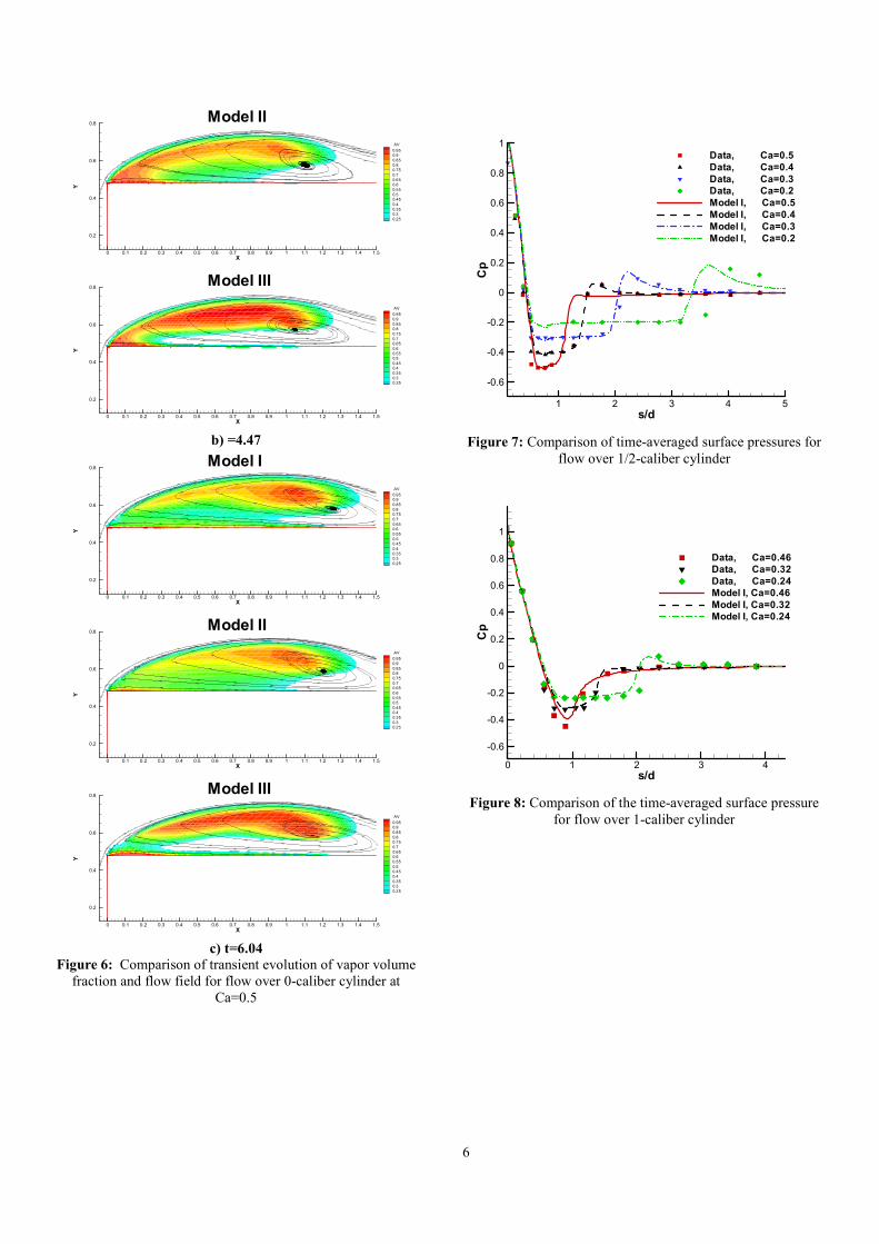
Figure 6 shows the comparison of transient plots of vapor

volume fraction contour against those predicted by Model II

and Model III. Clearly, the vapor distribution predicted by

Mode I at these dimensionless time instants agree very well

with those predicted by Model II. With Model III, the re-entrant

flow is more prominent. Since there is no difference between

growth and collapse of the bubble (Equation 14), Model III

produces a larger amount of vapor in the low pressure region

compared to Models I and II resulting in changes in the density

of the mixture and hence changes in pressure gradients. An

4

increase in adverse pressure gradient near the closure region of

the cavity has a direct impact on the development of the re-

entrant motion and causes the cavity to roll up and separate.

Figures 7 and 8 present the time-averaged surface pressure

distribution for the 1/2- and 1-caliber cylinders using Model I at

different cavitation numbers. For both configurations, the

results well capture the cavity pressure distribution and cavity

size.

The comparisons among the Model I, Model II, and Model

III are presented in Figures 9 and 10 for the flow over a 1/2

caliber cylinder at two cavitation numbers of 0.2 and 0.4,

respectively, and in Figures 11 and 12 for the flow over a 1-

caliber cylinder at two cavitation numbers of 0.24 and 0.32,

respectively. The computational results of Models I and II are

in close agreement with each other and with data while the

cavity length obtained by Model III is slightly smaller than the

one obtained by Model I and II. It should be noted that the

number density, N, may play the key control in Model III and it

should not be kept constant throughout the whole domain.

Keeping this number as a constant may not be sufficient to

accurately model the cavitation dynamics, as discussed in Ref.

[18].

(b) 1/2-caliber

(a) 0-caliber

(c) 1-caliber

Figure 1: Configurations of axisymmetric cylinder

s/d

Cp

0 2 4 6

-0.4

0

0.4

0.8

1.2

Data, Ca = 0.5

Data, Ca = 0.3

Model I, Ca = 0.5

Model I, Ca = 0.3

Owis & Neyfeh, Ca = 0.5

Owis & Neyfeh, Ca = 0.3

Figure 2: Comparison of time-averaged surface pressures for

flow over a 0-caliber cylinder

X

Y

0 0.5 1 1.50

0.2

0.4

0.6

0.8

AV

0.90.85

0.8

0.750.7

0.65

0.60.55

0.50.45

0.4

0.35

0.30.25

Kv=100.0; Kv/Kl=0.1

X

Y

0 0.5 1 1.50

0.2

0.4

0.6

0.8

AV

0.90.85

0.8

0.750.7

0.65

0.60.55

0.50.45

0.4

0.35

0.30.25

Kv=100.0; Kv/Kl=1.0

X

Y

0 0.5 1 1.50

0.2

0.4

0.6

0.8

AV

0.90.85

0.8

0.750.7

0.65

0.60.55

0.50.45

0.4

0.35

0.30.25

Kv=100.0; Kv/Kl=15.0

Figure 3: Vapor fraction contour and flow field for flow over a

0-caliber cylinder at Ca=0.5; t=7.0 (Model I)

5

X

Y

0 0.5 1 1.5 2 2.5 3

0.2

0.4

0.6

0.8

1

1.2

1.4

AV

0.9

0.85

0.8

0.75

0.7

0.65

0.6

0.55

0.5

0.45

0.4

0.35

0.3

0.25

0.2

Kv=0.1; Kv/Kl=10.0

X

Y

0 0.5 1 1.5 2 2.5 3

0.2

0.4

0.6

0.8

1

1.2

1.4

AV

0.9

0.85

0.8

0.75

0.7

0.65

0.6

0.55

0.5

0.45

0.4

0.35

0.3

0.25

0.2

Kv=1.0; Kv/Kl=10.0

X

Y

0 0.5 1 1.5 2 2.5 3

0.2

0.4

0.6

0.8

1

1.2

1.4

AV

0.9

0.85

0.8

0.75

0.7

0.65

0.6

0.55

0.5

0.45

0.4

0.35

0.3

0.25

0.2

Kv=10.0; Kv/Kl=10.0

X

Y

0 0.5 1 1.5 2 2.5 3

0.2

0.4

0.6

0.8

1

1.2

1.4

AV

0.9

0.85

0.8

0.75

0.7

0.65

0.6

0.55

0.5

0.45

0.4

0.35

0.3

0.25

0.2

Kv=100.0; Kv/Kl=10.0

Figure 4: Vapor fraction contour and flow field for flow over a

0-caliber cylinder at Ca=0.5; t=7.0 (Model I)

X

Y

0 0.5 1 1.5 2 2.5 3

0.2

0.4

0.6

0.8

1

1.2

1.4

AV

0.9

0.85

0.8

0.75

0.7

0.65

0.6

0.55

0.5

0.45

0.4

0.35

0.3

0.25

0.2

Cdest=1000.0; Cprod=0.10

X

Y

0 0.5 1 1.5 2 2.5 3

0.2

0.4

0.6

0.8

1

1.2

1.4

AV

0.9

0.85

0.8

0.75

0.7

0.65

0.6

0.55

0.5

0.45

0.4

0.35

0.3

0.25

0.2

Cdest=1000.0; Cprod=10.0

X

Y

0 0.5 1 1.5 2 2.5 3

0.2

0.4

0.6

0.8

1

1.2

1.4

AV

0.9

0.85

0.8

0.75

0.7

0.65

0.6

0.55

0.5

0.45

0.4

0.35

0.3

0.25

0.2

Cdest=100.0; Cprod=1.0

Figure 5: Vapor fraction contour and flow field for flow over a

0-caliber cylinder at Ca=0.5; t=6.5 (Mode II)

X

Y

0 0.1 0.2 0.3 0.4 0.5 0.6 0.7 0.8 0.9 1 1.1 1.2 1.3 1.4 1.5

0.2

0.4

0.6

0.8

AV

0.950.9

0.85

0.80.75

0.7

0.650.6

0.55

0.50.45

0.4

0.350.3

0.25

Model I

X

Y

0 0.1 0.2 0.3 0.4 0.5 0.6 0.7 0.8 0.9 1 1.1 1.2 1.3 1.4 1.5

0.2

0.4

0.6

0.8

AV

0.950.9

0.85

0.80.75

0.7

0.650.6

0.55

0.50.45

0.4

0.350.3

0.25

Model II

X

Y

0 0.1 0.2 0.3 0.4 0.5 0.6 0.7 0.8 0.9 1 1.1 1.2 1.3 1.4 1.5

0.2

0.4

0.6

0.8

AV

0.950.9

0.85

0.80.75

0.7

0.650.6

0.55

0.50.45

0.4

0.350.3

0.25

Model III

a) t=3.20

X

Y

0 0.1 0.2 0.3 0.4 0.5 0.6 0.7 0.8 0.9 1 1.1 1.2 1.3 1.4 1.5

0.2

0.4

0.6

0.8

AV

0.950.9

0.85

0.80.75

0.7

0.650.6

0.55

0.50.45

0.4

0.350.3

0.25

Model I

6

X

Y

0 0.1 0.2 0.3 0.4 0.5 0.6 0.7 0.8 0.9 1 1.1 1.2 1.3 1.4 1.5

0.2

0.4

0.6

0.8

AV

0.950.9

0.85

0.80.75

0.7

0.650.6

0.55

0.50.45

0.4

0.350.3

0.25

Model II

X

Y

0 0.1 0.2 0.3 0.4 0.5 0.6 0.7 0.8 0.9 1 1.1 1.2 1.3 1.4 1.5

0.2

0.4

0.6

0.8

AV

0.95

0.9

0.850.8

0.75

0.7

0.65

0.6

0.55

0.5

0.450.4

0.35

0.30.25

Model III

b) =4.47

X

Y

0 0.1 0.2 0.3 0.4 0.5 0.6 0.7 0.8 0.9 1 1.1 1.2 1.3 1.4 1.5

0.2

0.4

0.6

0.8

AV

0.95

0.9

0.85

0.8

0.75

0.7

0.650.6

0.55

0.50.45

0.4

0.35

0.3

0.25

Model I

X

Y

0 0.1 0.2 0.3 0.4 0.5 0.6 0.7 0.8 0.9 1 1.1 1.2 1.3 1.4 1.5

0.2

0.4

0.6

0.8

AV

0.95

0.9

0.85

0.8

0.75

0.70.65

0.6

0.550.5

0.45

0.4

0.35

0.3

0.25

Model II

X

Y

0 0.1 0.2 0.3 0.4 0.5 0.6 0.7 0.8 0.9 1 1.1 1.2 1.3 1.4 1.5

0.2

0.4

0.6

0.8

AV

0.95

0.9

0.85

0.80.75

0.7

0.650.6

0.55

0.5

0.45

0.4

0.35

0.3

0.25

Model III

c) t=6.04

Figure 6: Comparison of transient evolution of vapor volume

fraction and flow field for flow over 0-caliber cylinder at

Ca=0.5

s/d

Cp

1 2 3 4 5

-0.6

-0.4

-0.2

0

0.2

0.4

0.6

0.8

1

Data, Ca=0.5

Data, Ca=0.4

Data, Ca=0.3

Data, Ca=0.2

Model I, Ca=0.5

Model I, Ca=0.4

Model I, Ca=0.3

Model I, Ca=0.2

Figure 7: Comparison of time-averaged surface pressures for

flow over 1/2-caliber cylinder

s/d

Cp

0 1 2 3 4

-0.6

-0.4

-0.2

0

0.2

0.4

0.6

0.8

1

Data, Ca=0.46

Data, Ca=0.32

Data, Ca=0.24

Model I, Ca=0.46

Model I, Ca=0.32

Model I, Ca=0.24

Figure 8: Comparison of the time-averaged surface pressure

for flow over 1-caliber cylinder

7

s/d

Cp

0 1 2 3 4 5 6

-0.2

0

0.2

0.4

0.6

0.8

1

Data, Ca=0.2

Model I, Ca=0.2

Model II, Ca=0.2

Model III, Ca=0.2

(a)

X

Y

0 0.5 1 1.5 2 2.5

0

0.5

1

AV

0.95

0.90.85

0.8

0.75

0.70.65

0.6

0.550.5

0.45

0.4

0.350.3

0.25

Model I, Ca=0.2

X

Y

0 0.5 1 1.5 2 2.5

0

0.5

1

AV

0.950.9

0.85

0.80.75

0.7

0.65

0.60.55

0.5

0.45

0.40.35

0.3

0.25

Model II, Ca=0.2

X

Y

0 0.5 1 1.5 2 2.5

0

0.5

1

AV

0.95

0.90.85

0.8

0.75

0.70.65

0.6

0.55

0.5

0.450.4

0.35

0.3Model III, Ca=0.2

(b)

Figure 9: (a) Time-averaged surface pressures and

(b) predicted vapor volume fraction contour for 1/2-caliber

cylinder at t=47.1

s/d

Cp

0 0.5 1 1.5 2

-0.4

-0.2

0

0.2

0.4

0.6

0.8

1

Data, Ca=0.4

Model I, Ca=0.4

Model II, Ca=0.4

Model III, Ca=0.4

(a)

X

Y

-0.4 -0.2 0 0.2 0.4 0.6 0.80

0.1

0.2

0.3

0.4

0.5

0.6

AV

0.950.9

0.85

0.80.75

0.7

0.650.6

0.55

0.50.45

0.4

0.350.3

0.25

Model I, Ca=0.4

X

Y

-0.4 -0.2 0 0.2 0.4 0.6 0.80

0.1

0.2

0.3

0.4

0.5

0.6

AV

0.90.85

0.8

0.750.7

0.65

0.60.55

0.5

0.450.4

0.35

0.3

0.25

Model II, Ca=0.4

X

Y

-0.4 -0.2 0 0.2 0.4 0.6 0.80

0.1

0.2

0.3

0.4

0.5

0.6

AV

0.95

0.9

0.85

0.8

0.75

0.7

0.65

0.6

0.55

0.5

0.45

0.4

0.35

0.3

0.25

Model III, Ca=0.4

(b)

Figure 10: (a) Time-averaged surface pressures and

(b) predicted vapor volume fraction contours for 1/2-caliber

cylinder at t=24.3

8

s/d

Cp

0 1 2 3 4

-0.2

0

0.2

0.4

0.6

0.8

1

Data, Ca=0.24

Model I, Ca=0.24

Model II, Ca=0.24

Model III, Ca=0.24

(a)

X

Y

-1 -0.5 0 0.5 1

0

0.2

0.4

0.6

0.8

AV

0.950.9

0.85

0.8

0.750.7

0.65

0.60.55

0.5

0.45

0.40.35

0.3

0.25

Model I, Ca=0.24

X

Y

-1 -0.5 0 0.5 1

0

0.2

0.4

0.6

0.8

AV

0.950.9

0.85

0.8

0.750.7

0.65

0.6

0.550.5

0.45

0.4

0.350.3

0.25

Model II, Ca=0.24

X

Y

-1 -0.5 0 0.5 1

0

0.2

0.4

0.6

0.8

AV

0.95

0.9

0.85

0.8

0.75

0.7

0.65

0.6

0.55

0.5

0.45

0.4

0.35

0.3

Model III, Ca=0.24

(b)

Figure 11: (a) Time-averaged surface pressures and

(b) predicted vapor volume fraction contours for

1-caliber cylinder at t=50.3

s/d

Cp

0 0.5 1 1.5 2

-0.2

0

0.2

0.4

0.6

0.8

1

Data, Ca=0.32

Model I, Ca=0.32

Model II, Ca=0.32

Model III, Ca=0.32

(a)

X

Y

-0.2 0 0.2 0.4

0.3

0.4

0.5

0.6

AV

0.7

0.65

0.60.55

0.5

0.450.4

0.35

0.30.25

0.2

Model I, Ca=0.32

X

Y

-0.2 0 0.2 0.4

0.3

0.4

0.5

0.6

AV

0.7

0.650.6

0.55

0.50.45

0.4

0.350.3

0.25

0.2

Model II, Ca=0.32

X

Y

-0.2 0 0.2 0.4

0.3

0.4

0.5

0.6

AV

0.95

0.9

0.85

0.8

0.75

0.7

0.65

0.6

0.55

0.5

0.45

0.4

0.35

0.3

0.25

Model III, Ca=0.32

(b)

Figure 12: (a) Time-averaged surface pressures and

(b) predicted vapor volume fraction contours for

1-caliber cylinder at t=45.0

9

CONCLUSIONS A new cavitation model has successfully been validated for

different configurations under many flow conditions. The

model works stably. Like existing models, the new cavitation

model requires mass transfer model constants which play the

key role of controlling the mechanism of phase change. These

constants can easily be determined by numerical experiments.

Future work will focus on validation for more complex

configurations and take account into compressible fluids as

well as cavitation-induced turbulence effects.

ACKNOWLEDGMENTS

The authors gratefully acknowledge the support from

Underwater Vehicle Research Center (UVRC), Agency for

Defense Development (ADD), and Defense Acquisition

Program Administration (DAPA) of Korea.

NOMENCLATURE

Symbols

A, B, C convective Jacobian matrix

Av, B

v, C

v viscous Jacobian matrix

Ca

cavitation number,

2

v

Uρ2

1

ppCa

∞∞

∞ −=

Cdest, Cprod mass transfer model constants

S,Q,G,F,E,G,F,Evvv

flux vectors in ξ , η , and ζ

directions, solution vector, source

vector

f ramping function J Jacobian of the transformation

k scaling constant

L length scale −

m& , +m& evaporation and condensation rates

N bubble number density

p pressure

Re∞ Reynolds number,

l

l

µ

LρURe ∞

∞ =

t, t∞ time, characteristic time, t∞=L/U∞

u, v, w Cartesian velocity components

U, V, W contravariant velocities

α volume fraction

β preconditioning parameter

Γe, Γ flux Jacobian matrix, precondition

matrix

µ dynamic viscosity

ρ density

1ρ∆ density difference, v11 ρρρ −=∆

τ pseudo time, stress

Subscripts

L liquid

T turbulent

V vapor

∞ free stream value

REFERENCES [1] Reboud, J. L., Delannoy, Y., 1994, “ Two-phase flow

modeling of unsteady cavitation,” Proc. of 2nd

International Symposium on Cavitation, Tokyo, Japan,

39-44.

[2] Song, C., He, J., 1998, “Numerical simulation of

cavitating flows by single-phase flow approach,” Proc.

of 3rd International Symposium on Cavitation, Grenoble,

France, 295-300.

[3] Kunz, R. F., Lindau, J. W., Billet M. L., and Stinebring

D. R., “Multiphase CFD modeling of Developed and

Supercavitaing Flows,” Proceedings of the Von Karman

Institute Special Course on Supercavitating Flows, 12-16

February 2001, Rhode-Saint-Genese, Belgium.

[4] Kunz, R. F., Boger, D. A., Stinebring, D. R, Chyczewski,

T. S. , Lindau, J. W. , Gibeling H. J., Venkateswaran, S,

Govindan, T. R., 2000, ''A preconditioned Navier–Stokes

method for two-phase flows with application to

cavitation prediction,'' Computers and Fluids, Vol 29, pp.

849.

[5] Merkle, C. L., Feng, J. Z., Buelow, P. E. O., 1998,

“Computational Modeling of the Dynamics of Sheet

Cavitation”, Proc. of the 3rd International Symposium on

Cavitation, Grenoble, France, 307-311.

[6] Kunz, R. F., Boger, D. A., Stinebring, D. R, Chyczewski,

T. S. , Lindau, J. W. , Gibeling H. J., Venkateswaran, S,

Govindan, T. R., 2000, “A preconditioned Navier–Stokes

method for two-phase flows with application to

cavitation prediction”, Computers and Fluids, 29, 849-

875.

[7] Ahuja, V., Hosangadi, A., Arunajatesan, S., 2001,

“Simulation of Cavitating Flow Using Hybrid

Unstructured Meshes”, Jounal of Fluids Engineering,

123, 331-340.

[8] Shin, B. R., Itohagi, T., 1998, “A numerical study of

unsteady cavitaing flows,” Proc. of the 3rd International

Symposium on Cavitation, Grenoble, France, 301-306.

[9] W. Yuan, H.G. Schnerr, 2003, “Numerical simulation of

two-phase flow in injection nozzles: interaction of

cavitation and external jet formation”, Jounal of Fluids

Engineering, 125, 963–969.

[10] Grogger, H. A., Alajbegovic, A., 1998, “Calculation of

the cavitating flow in venture geometries using two fluid

model,” ASME Paper FEDSM 98-5295.

[11] Staedkte, H., Deconinck, H., and Romenski, E., 2005,

“Advanced three-dimensional two-phase flow simulation

tools for application reactor safety(ASTAR),” Nuclear

Engineering and Design, 235, 379-400.

[12] Merkle, C.L., Li, D., and Venkateswaran, S., 2006,

“Multi-Disciplinary computational analysis in

propulsion”, AIAA Paper 2006-4575.

[13] Yuan, W., Schnerr, H. G., 2003, “Numerical simulation

of two-phase flow in injection nozzles: interaction of

cavitation and external jet formation,” Jounal of Fluids

Engineering 125, 963–969.

[14] Payne, J. L. et al. "A Comparison of Turbulence Models

for a Supersonic Jet in Transonic Crossflow", AIAA

2001-1048,39th AIAA aerospace Sciences Meeting &

Exhibit.

10

[15] Chien K. Y., 1982, "Prediction of Change and Boundary

Layer Flows with a Low-Reynolds-Number Turbulence

Model,'' AIAA Journal, Vol.22, pp. 33-38.

[16] Rouse H., McNown J.S., ''Cavitation and Pressure

Distribution'', Head Forms at Zero Angle of Yaw, Stud.

Engrg., vol. 32, State University of Iowa, 1948.

[17] Owis F. M., Nayfeh A. H., 2003, ''Computational of

Compressible Multiphase Flow Over the Cavitating

High-Speed Torpedo'', Jounal of Fluids Engineering, Vol

125, 459-468.

[18] Srinivasan, V., Salazar, A. J., Saito, K., 2009,

“Numerical simulation of cavitation dynamics using a

cavitation-induced-momentum-defect (CIMD) correction

approach,” Applied Mathematical Modelling 33, 1529–

1559.

[19] Kunz, R., Boger, D., Chyczewski, T., Stinebring, D.,

Gibeling, H., 1999, "Multi-phase CFD analysis of natural

and ventilated cavitation about submerged bodies",

ASME FEDSM 99-7364, San Francisco.

[20] Venkateswarn, S., Lindau, J. W., Kunz, R.F., Merkle, C.

L., 2001, "Preconditioning Algorithms for Computation

of Multi-Phase Mixture Flows", AIAA 39th Aerospace

Sciences Meeting & Exhibit, AIAA Paper 2001-0279.