1

Multipath and Doppler Effects and Models There are two parts in this lecture.

• In Part I, we will first introduce the mutipath propagation effects and Doppler frequency shift/spread effects.

• In Part II, we will briefly introduce multipath and Doppler channel models.

2

Background: Overviews on Wireless Channel Modeling We need to ask the following three important questions while designing a wireless communication link:

1. Fading & Power Loss: Is the signal to interference plus noise ratio (SINR) large enough for the receiver

to detect the transmitted signal? 2. Signal Distortion: Can the signal distortion be ignored, predicted or removed so that we know how

to recover the transmitted information at the receiver? 3. Time Variation: Can the receiver adapt faster enough to the variations of the above two features

(SINR & signal distortion)?

A complete wireless channel model should provide quantitative measures of SINR, signal distortion and time variation.

For SINR (referred in question 1), we need only to consider the time invariant transmission loss at a single frequency (that is the RF carrier frequency). The frequency and time dependent properties of signal can be addressed in answering questions 2 and 3. Signal distortion (referred in question 2) is caused by the frequency dependent variations of the received signal strength and phase. The primary source of frequency dependent variations is multipath propagation. Here, we need only to consider time invariant situations and leave the time varying features to question 3. Motions of receivers, transmitters or wireless environments generate Doppler effects. With Doppler effects, signal frequencies shift and spread. These Doppler effects will cause time variations in the received signal strength and wave shape. This kind of time varying features is usually random and can be modeled as stochastic processes.

In order to addressing these three important issues, we divide wireless channel modeling into three parts:

• Transmission loss -single frequency (or narrowband signal) -time invariant environment (or short observation time period) • Frequency dependent channel impulse response or transfer function -multiple frequencies (or broadband signal) -time invariant environment (or short observation time period) • Time varying channel impulse response or transfer function -multiple frequencies (or broadband signal)

3

-time varying environment (or long observation time period) We have discussed transmission loss (including path loss, short term fading and long term fading) of a single frequency response in time invariant environments in the previous lecture. Both frequency dependent and time varying features of a channel impulse response (or transfer function) will be introduced in this lecture.

4

Part I: Multipath and Doppler Effects

After studying this note, students will be able to 1. Understand multipath channel effects in both time and frequency domains 2. Understand Doppler effects in both time and frequency domains 3. Understand multipath and Doppler effects in both time and frequency domains I. Multipath Channel Effects: Time Invariant Case (No Doppler effects) In wireless communication environments, a signal transmitted from the transmitter reaches the receiver through many different paths as illustrated in Figure 1.

Let s(t) is the transmitted signal. The received signal can then be written as a sum of multipath arrivals:

1 2 31

( ) ( ), ....L

i i Li

y t a s t τ τ τ τ τ=

= − ≤ ≤ ≤ ≤∑ (1)

Here, L is the total number of multipath arrivals, ai and τi are the amplitude and arrival time of the ith ray, respectively. A. s(t) is a time harmonic (i.e., single frequency or sinusoidal) signal Consider the transmitted signal ( ) j ts t e ω= . Then, the received signal is

( )

1 1( ) ( ) with ( )n n

L Lj t jj t

n nn n

y t a e H e H a eω τ ωτωω ω− −

= =

= = =∑ ∑ (2)

Figure 1: Multipath propagation

5

Here, ( )H ω is defined as the transfer function of the multipath environment. Note that the receiver signal y(t) remains as a time harmonic signal with the same angular frequency ω as the transmitted signal s(t). Thus, no distortion in wave shape has occurred during the transmission of s(t) through a time invariant multipath environment. However, the magnitude of the signal has been modified. The new magnitude is ( )H ω which is a function of angular frequency ω . We use the following matlab code to generate the Figure 2: ======================================================== clear all; % amplitudes of 7 multipath arrivals a=[0.6154 0.7919 0.9218 0.7382 0.1763 0.4057 0.9355]; % arrival times of 7 multipath arrivals t=[0.9169 0.4103 0.8936 0.0579 0.3529 0.8132 0.0099]; i=0; % frequency index for omega=0:0.05:100; % angular freuencies multipath_arrival=a.*exp(j*omega*t); i=i+1; abs_H(i)=abs(sum(multipath_arrival)); % the i-th transfer function end omega=0:0.05:100; plot(omega, abs_H) ylabel('amplitude of transfer function') xlabel('angular freuency') title('frequency dependent multipath fading') Here, we use 7 multipath arrivals. The amplitudes and arrival times of these seven multipath arrivals are randomly chosen. From Figure 2, the magnitude of received signal fluctuates as angular frequency changes. For some frequencies, the 7 multipath arrivals interfere destructively and yield small ( )H ω . For other frequencies, the 7 multipath

arrivals interfere constructively and yield large ( )H ω . This phenomenon is called multipath fading. Figure 2 shows that multipath fading is frequency dependent. Other kinds of fading will be discussed in future lectures.

6

Figure 2: Multipath fading is a function of frequency.

Since the amplitudes and arrival times of multipath arrivals depend on locations of transmitter and receiver, the received signal strength will also depend on the locations of transmitter and receiver. For example, consider a two ray model where line of sight (LOS) and reflected rays are the two multipath arrivals. Let the transmitter antenna height be ht and the receiver antenna height be hr. The horizontal distance between the transmitter and the receiver is denoted as d. From Figure 3, the travel distance for the LOS ray is

2 2( )LOS t rr d h h= + − and the travel distance for the reflected ray is

2 2( )ref t rr d h h= + + Then the transfer function is

/ 2 // 2 /( ) ref refLOS LOSj r c j rref refj r c j rLOS LOS

LOS ref LOS ref

b bb bH d e R e e Rer r r r

ω π λω π λ= + = +

7

where R is the reflection coefficient and the coefficients bLOS and bref are functions of antenna patterns, transmitted power, etc. For convenience, we choose bLOS =1, bref=1 and R=-1 in our example. Thus,

2 /2 /1 1( ) refLOS j rj r

LOS ref

H d e er r

π λπ λ= −

Figure 3: two-ray model

We will first plot the magnitude of ( )H d against the distance d using the following matlab code. If the frequency f=1GHz, the wave length is /c fλ = =0.3 m because the wave speed c=3*108m/sec. Let ht=10m, hr=2m. ============================================================= clear all ht=10;hr=2; c=3e8;f=1e9;lambda=c/f; R=-1; d=1:0.5:10000; d1=sqrt(d.^2+(ht-hr)^2); d2=sqrt(d.^2+(ht+hr)^2); a1=exp(j*2*pi.*d1/lambda)./d1; a2=R*exp(j*2*pi.*d2/lambda)./d2; a=abs(a1+a2); ld=log10(d);la=log10(a); figure (4) plot(ld,la); xlabel('log10(distance)') ylabel('log10(magnitude)') title( 'two ray model') ==============================================================

10m

d 2m

LOS

Reflected

8

Figure 4: Mutipath effects as a function of distance between source and receiver. Please see lecture 2 for detailed discussions. Secondly, we plot the magnitude of ( )H f against the frequency f for four distances d=50m, 300m, 800m and 2000m using the following matlab code: ============================================================= clear all ht=10;hr=2; c=3e8;R=-1; f0=1e8; fi= [1:1:1000];fd=5000000;f= f0+fd*fi; lambda=c./f; da=[50,300,800,2000]; for i=1:length(da) d=da(i); d1=sqrt(d.^2+(ht-hr)^2); d2=sqrt(d.^2+(ht+hr)^2); Td=(d2-d1)/c a1=exp(j*2*pi*d1./lambda)/d1; a2=R*exp(j*2*pi*d2./lambda)/d2; a(i,:)=abs(a1+a2); end figure (5)

9

subplot(2,2,1);plot(f,a(1,:));title('d=50m');ylabel('magnitude') subplot(2,2,2);plot(f,a(2,:));title('d=300m');ylabel('magnitude') subplot(2,2,3);plot(f,a(3,:)); title('d=800m');xlabel('frequency');ylabel('magnitude') subplot(2,2,4);plot(f,a(4,:)); title('d=2000m');xlabel('frequency');ylabel('magnitude') ==============================================================

Figure 5 Frequency characteristics of Multipath fading at four locations. From Figures 4 and 5, we conclude that frequency characteristics of Multipath fading are location dependent. Note that the frequency separation of two adjacent deep fades is in each case in Figure 5 is 1/TD where TD is the travel time difference for the two rays:

ref LOSr rTD

c−

=

10

B. s(t) contains multiple frequency components As shown in equation (2), the transfer function of a wireless communication channel with multipath arrivals can be written as

1( ) n

Lj

nn

H a e ωτω −

=

=∑

Here, an and nτ are the amplitude and time-delay of the nth ray, respectively. As shown in (1), for an input signal s(t) with multiple frequencies, the output of the channel can be written as

1

( ) ( )L

n nn

y t a s t τ=

= −∑

When the signal s(t) consists of multiple frequency components,

1( ) ( )2

j ts t S e dωω ωπ

∞

−∞= ∫ (3)

where ( )S ω is the spectrum of s(t). The spectrum of y(t) can be written as

1( ) ( ) ( ) ( ) n

Lj

nn

Y H S a S e ωτω ω ω ω −

=

= =∑ (4)

Consider the following 6-ray model as an example. The amplitudes are defined as an: [1, 0.3, -0.8, 0.5, -0.4, 0.2]. We will consider two kinds of arrival time distributions: Case 1: nτ : [0, 1µs, 2µs, 3µs, 4µs, 5µs] Case 2: nτ : [0, 0.1µs, 0.2µs, 0.3µs, 0.4µs, 0.5µs] The delay separation between the first arrival and the last arrival is 5µs in Case 1 and is only 0.5 µs in Case 2. For the time being, the delay separation is called as delay spread. In future lectures, delay spread will be defined in other ways. Consider the transmitted signal is a square pulse with pulse width equal to 5µs, 1. Time Domain View: We use the following matlab code to generate the time domain view of transmitted signals and received signals for both cases. From Figure 6, we observe that multipath arrivals cause distortion. The larger the delay spread is, the worse the distortion becomes.

11

clear all; an=[1,0.3,-0.8,0.5,-0.4,0.2];tn=[0,1,2,3,4,5;0,0.1,0.2,0.3,0.4,0.5]; signal=[0, zeros(1,0),ones(1,501),zeros(1,1000)]; % transmitted signal for k=1:2; %for two cases for i=1:6; ray(i,:)=an(i)*[0, zeros(1,(100*tn(k,i))),ones(1,501),zeros(1,(1000-100*tn(k,i)))]; end y(k,:)=sum(ray(:,1:end)); end t=((1:1:length(y(1,:)))-1)*10^(-2); subplot(2,2,1);plot(t,signal); ylabel('transmitted signal s(t)'); title('case 1 & case 2') axis([ 0 20 -0.5 1.5]) subplot(2,2,2);plot(t,y(1,:)); ylabel('received signal y(t)'); title('case 1: large delay spread') subplot(2,2,4); plot(t,y(2,:)); xlabel('Time(us)'); ylabel('received signal y(t)'); title('case 2: small delay spread')

12

Figure 6: Transmitted and received signals for two cases.

13

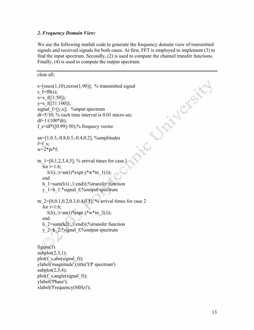
2. Frequency Domain View: We use the following matlab code to generate the frequency domain view of transmitted signals and received signals for both cases. At first, FFT is employed to implement (3) to find the input spectrum. Secondly, (2) is used to compute the channel transfer functions. Finally, (4) is used to compute the output spectrum. clear all; s=[ones(1,10),zeros(1,90)]; % transmitted signal s_f=fft(s); x=s_f([1:50]); y=s_f([51:100]); signal_f=[y,x]; %input spectrum dt=5/10; % each time interval is 0.01 micro sec df=1/(100*dt); f_s=df*([0:99]-50);% frequecy vector an=[1,0.3,-0.8,0.5,-0.4,0.2]; %amplitudes f=f_s; w=2*pi*f; tn_1=[0,1,2,3,4,5]; % arrival times for case 1 for i=1:6; h1(i,:)=an(i)*exp(-j*w*tn_1(i)); end h_1=sum(h1(:,1:end));%transfer function y_1=h_1.*signal_f;%output spectrum tn_2=[0,0.1,0.2,0.3,0.4,0.5]; % arrival times for case 2 for i=1:6; h2(i,:)=an(i)*exp(-j*w*tn_2(i)); end h_2=sum(h2(:,1:end));%transfer function y_2=h_2.*signal_f;%output spectrum figure(1) subplot(2,3,1); plot(f_s,abs(signal_f)); ylabel('magnitude');title('I/P spectrum') subplot(2,3,4); plot(f_s,angle(signal_f)); ylabel('Phase'); xlabel('Frequency(MHz)');

14

subplot(2,3,2); plot(f,abs(h_1)); title('channel 1') subplot(2,3,5); plot(f,angle(h_1)); xlabel('Frequency(MHz)'); subplot(2,3,3); plot(f,abs(h_2)); title('channel 2') subplot(2,3,6); plot(f,angle(h_2)); xlabel('Frequency(MHz)'); figure(2) subplot(2,3,1); plot(f_s,abs(signal_f)); ylabel('magnitude');title('I/P spectrum') subplot(2,3,4); plot(f_s,angle(signal_f)); ylabel('Phase'); xlabel('Frequency(MHz)'); subplot(2,3,2); plot(f,abs(y_1)); title('O/P spectrum 1') subplot(2,3,5); plot(f,angle(y_1)); xlabel('Frequency(MHz)'); subplot(2,3,3); plot(f,abs(y_2)); title('O/P spectrum 2') subplot(2,3,6); plot(f,angle(y_2)); xlabel('Frequency(MHz)'); ===============================================================

15

The input spectrum and channel functions for both cases are shown in Figure 7. The magnitude functions are on the top row and the phase functions are on the bottom row. From the left column, one can see the input spectrum lies primarily in [-200kHz 200kHz]. For channel 2 (right column), the magnitude of transfer function is basically flat and the phase of the transfer function is basically linear in this interval. Therefore, channel 2 will cause little distortion and this kind of channel is called to have flat fading. For channel 1 (center column), the magnitude of transfer function is not flat and the phase of the transfer function is not linear in this interval. Therefore, channel 1 will cause more distortion and this kind of channel is called to have frequency selective fading.

Figure 7: Input spectrum (left column), transfer function of case 1 (center column), and transfer function of case 2 (right column).

16

The input spectrum and output spectra for both cases are shown in Figure 8. The magnitude functions are on the top row and the phase functions are on the bottom row. The input spectrum, shown in the left column, is the same as that in Figure 7. As mentioned before, it lies primarily in [-200kHz 200kHz]. For channel 2, the output spectrum (right column) is very similar to the input spectrum. Therefore, channel 2 will cause little distortion and this kind of channel is called to have flat fading. For channel 1, the output spectrum (right column) is not similar to the input spectrum. Therefore, channel 1 will cause more distortion and this kind of channel is called to have frequency selective fading.

Figure 8: Input spectrum (left column), output spectrum of case 1 (center column), and output spectrum of case 2 (right column). From Figures 7, the variation rate (with respect to frequency) of the transfer function is proportional to the delay spread. A larger delay spread causes a faster variation rate in the transfer function. This is illustrated by Figure 9 where the absolute value of the transfer functions for four delay spreads are plotted against the frequency. The code of generating this figure is also shown below. For the case with delay spread=0.2 µ sec, a cycle of variation (from a local peak to the next local peak) is of the order of 5 MHz. Similarly, for the case with delay spread=1 µ sec, 5 µ sec, or 10 µ sec , a cycle of

17

variation (from a local peak to the next local peak) is of the order of 1 MHz, 0.2 MHz, or 0.1 MHz, respectively.

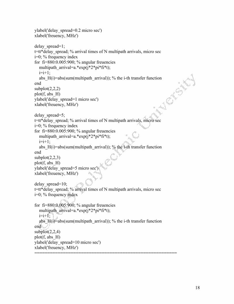
Figure 9 Absolute values of the transfer functions of four delay spreads. clear all; N=20 %number of rays a=rand(1,N); % amplitudes of N multipath arrivals tt=rand(1,N); f=880:0.005:900; delay_spread=0.2; t=tt*delay_spread; % arrival times of N multipath arrivals, micro sec i=0; % frequency index for fi=880:0.005:900; % angular freuencies multipath_arrival=a.*exp(j*2*pi*fi*t); i=i+1; abs_H(i)=abs(sum(multipath_arrival)); % the i-th transfer function end subplot(2,2,1) plot(f, abs_H)

18

ylabel('delay_spread=0.2 micro sec') xlabel('freuency, MHz') delay_spread=1; t=tt*delay_spread; % arrival times of N multipath arrivals, micro sec i=0; % frequency index for fi=880:0.005:900; % angular freuencies multipath_arrival=a.*exp(j*2*pi*fi*t); i=i+1; abs_H(i)=abs(sum(multipath_arrival)); % the i-th transfer function end subplot(2,2,2) plot(f, abs_H) ylabel('delay_spread=1 micro sec') xlabel('freuency, MHz') delay_spread=5; t=tt*delay_spread; % arrival times of N multipath arrivals, micro sec i=0; % frequency index for fi=880:0.005:900; % angular freuencies multipath_arrival=a.*exp(j*2*pi*fi*t); i=i+1; abs_H(i)=abs(sum(multipath_arrival)); % the i-th transfer function end subplot(2,2,3) plot(f, abs_H) ylabel('delay_spread=5 micro sec') xlabel('freuency, MHz') delay_spread=10; t=tt*delay_spread; % arrival times of N multipath arrivals, micro sec i=0; % frequency index for fi=880:0.005:900; % angular freuencies multipath_arrival=a.*exp(j*2*pi*fi*t); i=i+1; abs_H(i)=abs(sum(multipath_arrival)); % the i-th transfer function end subplot(2,2,4) plot(f, abs_H) ylabel('delay_spread=10 micro sec') xlabel('freuency, MHz') =======================================================

19

II. Doppler Effect & Multipath Effects

A. Doppler Frequency Shift (single path)

Denote the speed and the frequency of a radio wave as c and f, respectively. Define a wavefront as a surface with a constant phase. For example, consider a spherical wave

2 ( / ) /j f r c te rπ − emitted by a stationary source. The phase term is 2 ( / )f r c tπ − and a wavefront (a constant phase surface) can be defined as 2 ( / )f r c t aπ − = . Here, a is a constant. For any t, the wavefront is a sphere located at ( )/ 2r c t a fπ= + (see Figure 10). Note that the wavefront travels with the speed c. Let two adjacent wavefronts be defined as 2 ( / )f r c t aπ − = and 2 ( '/ ) 2f r c t aπ π− = − . Since ( 2 )ja j ae e π−= , the wavelength can then be defined as the distance between these two wavefronts (for any time t):

' /r r c fλ = − = .

Figure 10 Wavefronts of a stationary source

1. Moving Source (single path)

Doppler frequency shift due to a moving source can be explained by the following scenario. When an ambulance, police car, or fire truck races by you, the sound pitch emitted by the vehicle changes as the vehicle races towards, then away from you. This change in pitch results from a frequency shift of the sound waves (see Figure 11). As the vehicle approaches, the sound waves from its siren are compressed towards the listener. The intervals between waves diminish, which translates into an increase in frequency or pitch. As the vehicle recedes, the sound waves are stretched relative to the listener, causing the siren's pitch to decrease.

By analogy, the radio wave radiation emitted by a moving object also exhibits the Doppler frequency shift. The radiation emitted by an object moving toward an observer is

20

squeezed and its frequency appears to increase. In contrast, the radiation emitted by an object moving away is stretched and its frequency appears to decrease.

Figure 11: Doppler frequency shift of a moving source

Now consider the radiation source is moving with a speed v toward the receiver. Denote the location of the radiation source at t=0 as r=0. The wavefront radiated at t=0 is a sphere centered at r=0. The next wavefront will be radiated at 1/t f= (i.e., one cycle after the previous wavefront is radiated). As shown in Figure 11, since the radiation source is moving with a speed v, the source location at 1/t f= is r=v/f . In other words, this second wavefront will be a sphere centered at r=v/f. Therefore, the wavelength observed at the receiver is compressed by an amount of v/f and the equivalent wavelength is

/ / /v v f c f v fλ λ= − = − . Thus, the equivalent frequency observed at the observed becomes

1/ (1 )/ / 1

v vc vf c f fvc f v f c

c

λ= = = ≈ +− −

The Doppler shift frequency is

( )vvf f fc

− ≈

2. Moving Observer (single path) When the radiation source is stationary, wavefronts at t=0 are previously shown in Figure 10. The distance between two adjacent wavefronts is λ . These wavefronts propagate outward (away from the source) with a speed of c. If the observer is moving toward the source with a speed v, the relative speed between the wavefronts and the observer is v+c. Thus, the time for the observer to pass through a wavelength is

21

/v

c ftc v c vλ

= =+ +

and the equivalent frequency is

1 (1 )/v

v

c v vf ft c f c

+= = = +

Thus, the Doppler shift frequency is also

( )vvf f fc

− ≈

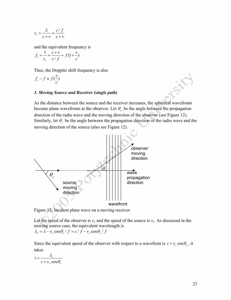
3. Moving Source and Receiver (single path) As the distance between the source and the receiver increases, the spherical wavefronts become plane wavefronts at the observer. Let oθ be the angle between the propagation direction of the radio wave and the moving direction of the observer (see Figure 12). Similarly, let sθ be the angle between the propagation direction of the radio wave and the moving direction of the source (also see Figure 12).

Figure 12: Incident plane wave on a moving receiver Let the speed of the observer is vo and the speed of the source is vs. As discussed in the moving source case, the equivalent wavelength is

cos / / cos /v s s s sv f c f v fλ λ θ θ= − = − Since the equivalent speed of the observer with respect to a wavefront is coso oc v θ+ , it takes

cosv

o o

tc v

λθ

=+

wavefront

wave propagation direction

observer moving direction

oθ

source moving direction

sθ

22

for the observer to pass from one wavefront to the next wavefront. If the speeds sv and

ov are much smaller than c, the Doppler shifted frequency is approximated as cos cos 1 cos /1

/ cos / 1 cos /(1 cos / )(1 cos / ) (1 cos / cos / )

o o o o o os o

v s s s s

o o s s o o s s

c v c v v cf ft c f v f v c

f v c v c f v c v c

θ θ θλ θ θ

θ θ θ θ

++ + −

= = = =− −

≈ + + ≈ + +

Thus, the Doppler frequency shift induced by a moving source and/or a moving receiver is

cos cos( )s s o ov

v vf f f fc

θ θ+∆ = − ≈ (5)

For a signal s(t), its spectrum

( ) ( ) j tS s t e dtωω∞ −

−∞= ∫ (6)

Having a frequency shift of f∆ , the new signal becomes

1( ) ( 2 )2

j tfs t S f e dωω π ω

π∞

∆ −∞= + ∆∫ (7)

If s(t) is a single frequency signal (say 2( ) j fts t e π= ), 2 ( )( ) j f f t

fs t e π +∆∆ = .

B. Doppler Frequency Shifts of a Time Harmonic Signal (Multipath)

As shown in Figure 1, multipath signals emit from the source at different angles and arrive at the observer at different angles. Thus, Doppler shifts of different arrivals are usually different from one another. For convenience and without loss of generality, let the relative speed between the source and the receiver is v to account for both vs and vo in (5). Since the range of cos is within -1 and +1, the maximum Doppler frequency shift is

Dvf fc

± = (8)

When there is no Doppler effect, as shown in (2), the received signal is

1

( ) ( ) with ( ) n

Njj t

nn

y t H e H a e ωτωω ω −

=

= =∑

Here, N is the total number of multipath arrivals, an and τn are the amplitude and arrival time of the nth ray, respectively. When there is Doppler effect, let 2n nfω π= , n Df f≤ , be the Doppler angular frequency shift of the nth ray. The received signal becomes

1

( ) ( , ) where ( , ) n n

Nj j tj t

nn

y t H t e H t a e ωτ ωωω ω − +

=

= =∑ (9)

is a time varying transfer function which is no longer a time harmonic signal.

23

Using the following matlab program, we generate Figure 13. clear all; N=20 ;% number of multipath arrivals a=rand(1,N); %amplitude tau=rand(1,N); %arrival time f_d=1 shift=rand(1,N)*2*f_d-f_d; %Doppler shifts f=10; % the frequency of the transmitted time harmonic signal f_shift=f+shift; t=[22:0.01:25]; %No Doppler shift s_t=exp(j*2*pi*f*t); %transmitted signal y_t=sum(a.*exp(-j*2*pi*f*tau))*exp(j*2*pi*f*t); %received signal n=1; y_d_t=sum(a(n)*exp(-j*2*pi*f*tau(n)))*exp(j*2*pi*(f_shift(n))*t); for n=2:N y_d_t=y_d_t+a(n)*exp(-j*2*pi*f*tau(n))*exp(j*2*pi*(f_shift(n))*t); %received signal end figure (1) subplot(2,2,3) stem(f_shift,a) xlabel('frequency, Hz') ylabel('ray amplitude') title('Doppler Shifts') subplot(2,2,2) plot(t,y_t,'r') title('no Doppler shift') ylabel('received signal') xlabel('time, sec') subplot(2,2,1) stem(tau,a) xlabel('Time, Sec') ylabel('ray amplitude') title('Time Delay') subplot(2,2,4) plot(t,y_d_t) title('with Doppler shifts') ylabel('received signal') xlabel('time, sec')

24

Here, a time harmonic signal with f=10Hz is transmitted. There are 20 multipath arrivals (rays). The randomly generated amplitudes and arrival times of the 20 rays are shown in the upper left graph. When there are no Doppler shifts, a portion of the received signal is shown in the upper right graph. One can see that the received signal is still a time harmonic signal with f=10Hz. There is no distortion. When there are Doppler frequency shifts, the randomly generated amplitudes and Doppler shifted frequencies of the 20 rays are shown in the lower left graph. A portion of the received signal is shown in the lower right graph. The signal is distorted and varies as time increases.

Figure 13 Multipath effect (without Doppler shifts) on a time harmonic signal and combined multipath and Doppler effects on a time harmonic signal. The variation rate (with respect to time) of the envelope of the time varying signal is proportional to the Doppler spread. A larger Doppler spread causes a faster variation in the envelope of the time varying signal. This is illustrated by Figure 14 where the envelope of the time varying signal for four Doppler spreads is plotted against the time. The code of generating this figure is also shown below. For the case with Doppler spread=0.01Hz, a cycle of variation (from a local peak to the next local peak) is of the order of 100 sec. Similarly, for the case with delay spread=0.05 Hz, 0.1 Hz, or 0.5 Hz, a

25

cycle of variation (from a local peak to the next local peak) is of the order of 20 sec, 10 sec, or 2 sec, respectively.

Figure 14: The received signal of a time varying channel where the transmitted signal is a time-harmonic signal with frequency f=10Hz. clear all; N=20 ;% number of multipath arrivals a=rand(1,N); %amplitude tau=rand(1,N); %arrival time f_d=0.01 shift=rand(1,N)*2*f_d-f_d; %Doppler shifts f=10; % the frequency of the transmitted time harmonic signal f_shift=f+shift; t=[0:0.01:50]; n=1; y_d_t=sum(a(n)*exp(-j*2*pi*f*tau(n)))*exp(j*2*pi*(f_shift(n))*t); for n=2:N

26

y_d_t=y_d_t+a(n)*exp(-j*2*pi*f*tau(n))*exp(j*2*pi*(f_shift(n))*t); %received signal end subplot(2,2,1) plot(t,y_d_t) xlabel('time, sec') ylabel('f_D=0.01') N=20 ;% number of multipath arrivals a=rand(1,N); %amplitude tau=rand(1,N); %arrival time f_d=0.05 shift=rand(1,N)*2*f_d-f_d; %Doppler shifts f=10; % the frequency of the transmitted time harmonic signal f_shift=f+shift; t=[0:0.01:50]; n=1; y_d_t=sum(a(n)*exp(-j*2*pi*f*tau(n)))*exp(j*2*pi*(f_shift(n))*t); for n=2:N y_d_t=y_d_t+a(n)*exp(-j*2*pi*f*tau(n))*exp(j*2*pi*(f_shift(n))*t); %received signal end subplot(2,2,2) plot(t,y_d_t) xlabel('time, sec') ylabel('f_D=0.05') N=20 ;% number of multipath arrivals a=rand(1,N); %amplitude tau=rand(1,N); %arrival time f_d=0.1 shift=rand(1,N)*2*f_d-f_d; %Doppler shifts f=10; % the frequency of the transmitted time harmonic signal f_shift=f+shift; t=[0:0.01:50]; n=1; y_d_t=sum(a(n)*exp(-j*2*pi*f*tau(n)))*exp(j*2*pi*(f_shift(n))*t); for n=2:N y_d_t=y_d_t+a(n)*exp(-j*2*pi*f*tau(n))*exp(j*2*pi*(f_shift(n))*t); %received signal

27

end subplot(2,2,3) plot(t,y_d_t) xlabel('time, sec') ylabel('f_D=0.1') N=20 ;% number of multipath arrivals a=rand(1,N); %amplitude tau=rand(1,N); %arrival time f_d=0.5 shift=rand(1,N)*2*f_d-f_d; %Doppler shifts f=10; % the frequency of the transmitted time harmonic signal f_shift=f+shift; t=[0:0.01:50]; n=1; y_d_t=sum(a(n)*exp(-j*2*pi*f*tau(n)))*exp(j*2*pi*(f_shift(n))*t); for n=2:N y_d_t=y_d_t+a(n)*exp(-j*2*pi*f*tau(n))*exp(j*2*pi*(f_shift(n))*t); %received signal end subplot(2,2,4) plot(t,y_d_t) xlabel('time, sec') ylabel('f_D=0.5') ==============================================================

28

C. Doppler and Multipath Effects of Signals with Multiple Frequencies In a time varying (i.e., with Doppler effect) multipath environment, as shown in (9), the received signal (due to a transmitted time harmonic signal j te ω ) is

1

( ) ( , ) where ( , ) n n

Nj j tj t

nn

y t H t e H t a e ωτ ωωω ω − +

=

= =∑

is the time varying spectrum. Consider a signal with multiple frequency components

1( ) ( )2

j ts t S e dωω ωπ

∞

−∞= ∫

The time varying spectrum of the received signal is ( ) ( , )S H tω ω and the time-domain received signal is

( )

1

( )

1 1

1 1( ) ( ) ( , ) ( )2 2

1 ( ) ( )2

n n

n n n

Nj t j tj t

nn

N Nj t j t j t

n n nn n

y t S H t e d a S e d

a S e d e a s t e

ω τ ωω

ω τ ω ω

ω ω ω ω ωπ π

ω ω τπ

∞ ∞ − +

−∞ −∞=

∞ −

−∞= =

= =

= ≈ −

∑∫ ∫

∑ ∑∫

In the first example, consider 2 cases with different Doppler spreads. In each case, there are 6 rays and the ray amplitudes of these 6 rays are an: [1, 0.3, -0.8, 0.5, -0.4, 0.2] The Doppler shifts are Case 1: ωn: [0, 2Hz, 10Hz, 6Hz, 8Hz, 4Hz] Case 2: ωn: [0, 20Hz, 100Hz, 60Hz, 80Hz, 40Hz] Here, we artificially make all travel time delays zero ( nτ =0). Consider s(t) is 1 between t0 to t0+5µs and is zero elsewhere. Plot y(t) for two observation times t0=0sec and 20msec in Figure 15. We observe that, at first, there is no distortion at the receiver because all travel time delays are zero ( nτ =0). Secondly, Doppler spread causes the signal to vary with time. At different observation times, the received signals are different. Thirdly, a larger Doppler spread causes a faster time variation rate. The code to generate Figure 15 is listed below. ========================================================= clear; t=(0:0.01:10);an=[1,0.3,-0.8,0.5,-0.4,0.2];wn=[0,2,10,6,8,4]; for i=1:6; s1(i,:)=an(i)*exp(j*0*wn(i))*[ones(1,501),zeros(1,500)]; s2(i,:)=an(i)*exp(j*0.02*wn(i))*[ones(1,501),zeros(1,500)]; end y1(1,:)=sum(s1);y2(1,:)=sum(s2);wn1=[0,20,100,60,80,40]; for k=1:6;

29

s3(k,:)=an(k)*exp(j*0*wn1(k))*[ones(1,501),zeros(1,500)]; s4(k,:)=an(k)*exp(j*0.02*wn1(k))*[ones(1,501),zeros(1,500)]; end y3(1,:)=sum(s3);y4(1,:)=sum(s4); subplot(2,1,1); plot(t,abs(y1));ylabel('y(t)'); xlabel('Time(us)'); title('case 1: small Doppler spread') ylim([-0.2 2.2]);hold on; plot(t,abs(y2),'r');hold off legend('t_0=0msec','t_0=20msec') subplot(2,1,2); plot(t,abs(y3));xlabel('Time(us)');ylabel('y(t)'); title('case 2: large Doppler spread') ylim([-0.2 2.2]);hold on; plot(t,abs(y4) ,'r');hold off legend('t_0=0msec','t_0=20msec') ============================================================

Figure 15: Doppler effects on a signal with multiple frequency components.

30

Continued from the previous example, we will consider non-zero travel time delays. Consider 4 cases with different combinations of delay spreads and Doppler spreads. In each case, there are 6 rays and the ray amplitudes of these 6 rays are an: [1, 0.3, -0.8, 0.5, -0.4, 0.2] The Doppler shifts are Cases 1 and 3 are with small Doppler spread: ωn: [0, 2Hz, 10Hz, 6Hz, 8Hz, 4Hz] Cases 2 and 4 are with large Doppler spread: ωn: [0, 20Hz, 100Hz, 60Hz, 80Hz, 40Hz] The travel time delays are Cases 1 and 2 are with large delay spread: nτ : [0, 1µs, 2µs, 3µs, 4µs, 5µs]; Cases 3 and 4 are with small delay spread: nτ : [0, 0.1µs, 0.2µs, 0.3µs, 0.4µs, 0.5µs]; We will discuss the frequency-domain view first. We use the following matlab code to compute and plot in Figure 16 the transfer function (amplitude and phase) for frequencies from –1MHz to +1MHz for two the observation times at t0 =0sec and 20msec. clear; an=[1,0.3,-0.8,0.5,-0.4,0.2]; tn=[0,1,2,3,4,5;0,1,2,3,4,5;0,0.1,0.2,0.3,0.4,0.5;0,0.1,0.2,0.3,0.4,0.5]; wn=[0,2,10,6,8,4;0,20,100,60,80,40;0,2,10,6,8,4;0,20,100,60,80,40]; f=-1:0.01:1; w=2*pi*f; for k=1:4; for i=1:6; h1(i,:)=an(i)*exp(-j*w*tn(k,i))*exp(j*wn(k,i)*0); h2(i,:)=an(i)*exp(-j*w*tn(k,i))*exp(j*wn(k,i)*0.02); end h1_1(k,:)=sum(h1(:,1:end)); h1_2(k,:)=sum(h2(:,1:end)); end subplot(4,2,1);plot(f,abs(h1_1(1,:)));ylabel('case 1');ylim([0 4]); hold on plot(f,abs(h1_2(1,:)) ,'r');title('amplitude'); %legend('t_0=0msec','t_0=20msec') hold off subplot(4,2,2);plot(f,angle(h1_1(1,:))); ylim([-4 4]); hold on plot(f,angle(h1_2(1,:)) ,'r'); title('phase'); % hold off subplot(4,2,3);plot(f,abs(h1_1(2,:)));ylabel('case 2');ylim([0 4]); hold on plot(f,abs(h1_2(2,:)) ,'r'); hold off subplot(4,2,4);plot(f,angle(h1_1(2,:)));ylim([-4 4]); hold on plot(f,angle(h1_2(2,:)) ,'r'); hold off

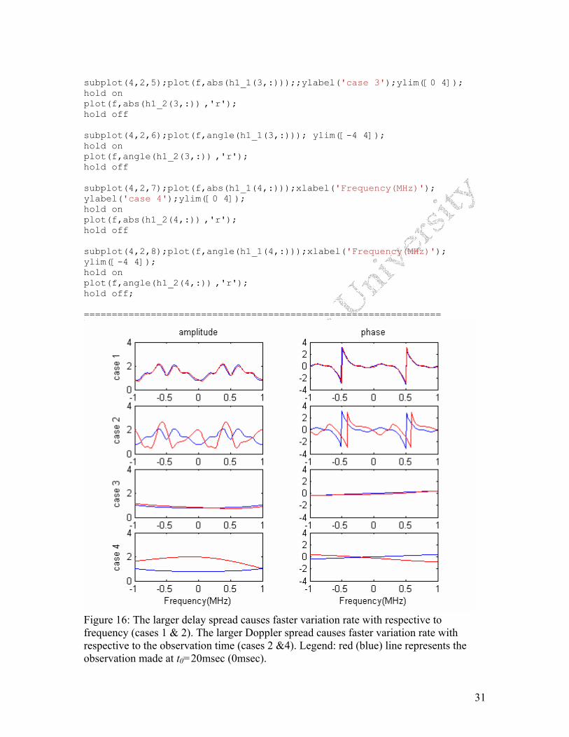
31

subplot(4,2,5);plot(f,abs(h1_1(3,:)));;ylabel('case 3');ylim([0 4]); hold on plot(f,abs(h1_2(3,:)) ,'r'); hold off subplot(4,2,6);plot(f,angle(h1_1(3,:))); ylim([-4 4]); hold on plot(f,angle(h1_2(3,:)) ,'r'); hold off subplot(4,2,7);plot(f,abs(h1_1(4,:)));xlabel('Frequency(MHz)'); ylabel('case 4');ylim([0 4]); hold on plot(f,abs(h1_2(4,:)) ,'r'); hold off subplot(4,2,8);plot(f,angle(h1_1(4,:)));xlabel('Frequency(MHz)'); ylim([-4 4]); hold on plot(f,angle(h1_2(4,:)) ,'r'); hold off; ================================================================

Figure 16: The larger delay spread causes faster variation rate with respective to frequency (cases 1 & 2). The larger Doppler spread causes faster variation rate with respective to the observation time (cases 2 &4). Legend: red (blue) line represents the observation made at t0=20msec (0msec).

32

Now we will discuss the time-domain view. Consider s(t) is 1 between t0 to t0+5µs and is zero elsewhere. We use the following matlab code to compute and plot in Figure 17 the received signal y(t) for the two observation times at t0 =0sec and 20msec. clear all; an=[1,0.3,-0.8,0.5,-0.4,0.2]; tn=[0,1,2,3,4,5;0,1,2,3,4,5;0,0.1,0.2,0.3,0.4,0.5;0,0.1,0.2,0.3,0.4,0.5]; wn=[0,2,10,6,8,4;0,20,100,60,80,40;0,2,10,6,8,4;0,20,100,60,80,40]; for k=1:4; for i=1:6; s1(i,:)=an(i)*exp(j*0*wn(k,i))*[zeros(1,(100*tn(k,i))),ones(1,501),zeros(1,(1000-100*tn(k,i)))]; s2(i,:)=an(i)*exp(j*0.02*wn(k,i))*[zeros(1,(100*tn(k,i))),ones(1,501),zeros(1,(1000-100*tn(k,i)))]; end y1(k,:)=sum(s1(:,1:end)); y2(k,:)=sum(s2(:,1:end)); end t=((1:1:length(y1(1,:)))-1)*10^(-2); subplot(4,2,1);plot(t,real(y1(1,:)));ylabel('case 1');ylim([-2 2]); hold on plot(t,real(y2(1,:)),'r');title('real part') hold off subplot(4,2,2);plot(t,imag(y1(1,:)));ylim([-2 2]); hold on plot(t,imag(y2(1,:)),'r');title('imaginary part') hold off subplot(4,2,3);plot(t,real(y1(2,:)));ylabel('case 2');ylim([-2 2]); hold on plot(t,real(y2(2,:)),'r'); hold off subplot(4,2,4);plot(t,imag(y1(2,:)));ylim([-2 2]); hold on plot(t,imag(y2(2,:)),'r'); hold off subplot(4,2,5);plot(t,real(y1(3,:)));;ylabel('case 3');ylim([-2 2]); hold on plot(t,real(y2(3,:)),'r'); hold off subplot(4,2,6);plot(t,imag(y1(3,:)));ylim([-2 2]);

33

hold on plot(t,imag(y2(3,:)),'r'); hold off subplot(4,2,7);plot(t,real(y1(4,:)));xlabel('Time(us)');ylabel('case 4'); hold on plot(t,real(y2(4,:)),'r');ylim([-2 2]); hold off subplot(4,2,8);plot(t,imag(y1(4,:)));xlabel('Time(us)');ylim([-2 2]); hold on plot(t,imag(y2(4,:)),'r');

Figure 17: The larger delay spread causes more distortion (cases 1 & 2). The larger Doppler spread causes faster variation rate with respective to the observation time (cases 2 &4). Legend: red (blue) line represents the observation made at t0=20msec (0msec). Results in Figures. 16 & 17 will be re-plotted in below with five observations: t0=0sec, 10msec, 20msec, 30msec, 40msec, and 50msec.

34

Case 1: an: [1, 0.3, -0.8, 0.5, -0.4, 0.2]; tn: [0, 1µs, 2µs, 3µs, 4µs, 5µs]; ωn: [0, 2Hz, 4Hz, 6Hz, 8Hz, 10Hz]

Part a: ∑=

−−=N

n

ttjn

nneatH1

)(),( ωωω Part b: )(

1

)()( tjN

nnn

nettsaty ω∑=

−=

-1 -0.5 0 0.5 10.5

1

1.5

2

2.5

MHz

|H(w)|

-1 -0.5 0 0.5 1-6

-4

-2

0

2

MHz

phase(H(w))

π

0 0.5 1 1.5

x 10-5

-0.5

0

0.5

1

1.5real(y(t))

0 0.5 1 1.5

x 10-5

-0.6

-0.4

-0.2

0

0.2

0.4

sec

imag(y(t))

Doppler spread is not large (with respect to the time interval between observation times, i.e., ∆t0): Frequency Domain View: slow time selective fading Time Domain View: Time variation is slow Delay spread is large (with respect to symbol duration): Frequency Domain View: Frequency selective fading is severe Time Domain View: Distortion is severe.

35

Case 2: an: [1, 0.3, -0.8, 0.5, -0.4, 0.2]; tn: [0, 1µs, 2µs, 3µs, 4µs, 5µs]; ωn: [0, 20Hz, 40Hz, 60Hz, 80Hz, 100Hz]

Part a: ∑=

−−=N

n

ttjn

nneatH1

)(),( ωωω Part b: )(

1

)()( tjN

nnn

nettsaty ω∑=

−=

-1 -0.5 0 0.5 10.5

1

1.5

2

2.5

MHz

|H(w)|

-1 -0.5 0 0.5 1-6

-4

-2

0

2

MHz

phase(H(w))

π

0 0.5 1 1.5

x 10-5

-0.5

0

0.5

1

1.5

2real(y(t))

0 0.5 1 1.5

x 10-5

-2

-1

0

1

2

sec

imag(y(t))

Doppler spread is large (with respect to the time interval between observation times, i.e., ∆t0): Frequency Domain View: fast time selective fading Time Domain View: Time variation is fast Delay spread is large (with respect to symbol duration): Frequency Domain View: Frequency selective fading is severe Time Domain View: Distortion is severe.

36

Case 3: an: [1, 0.3, -0.8, 0.5, -0.4, 0.2]; tn: [0, 0.1µs, 0.2µs, 0.3µs, 0.4µs, 0.5µs]; ωn: [0, 2Hz, 4Hz, 6Hz, 8Hz, 10Hz]

Part a: ∑=

−−=N

n

ttjn

nneatH1

)(),( ωωω Part b: )(

1

)()( tjN

nnn

nettsaty ω∑=

−=

-1 -0.5 0 0.5 10.8

1

1.2

1.4

1.6

MHz

|H(w)|

-1 -0.5 0 0.5 1-0.2

-0.1

0

0.1

0.2

MHz

phase(H(w))

π

0 0.5 1 1.5

x 10-5

-0.5

0

0.5

1

1.5real(y(t))

0 0.5 1 1.5

x 10-5

-0.6

-0.4

-0.2

0

0.2

0.4

sec

imag(y(t))

Doppler spread is not large (with respect to the time interval between observation times, i.e., ∆t0): Frequency Domain View: slow time selective fading Time Domain View: Time variation is slow Delay spread is small (with respect to symbol duration): Frequency Domain View: Frequency selective fading is not severe Time Domain View: Distortion is not severe.

37

Case 4: an: [1, 0.3, -0.8, 0.5, -0.4, 0.2]; tn: [0, 0.1µs, 0.2µs, 0.3µs, 0.4µs, 0.5µs]; ωn: [0, 20Hz, 40Hz, 60Hz, 80Hz, 100Hz]

Part a: ∑=

−−=N

n

ttjn

nneatH1

)(),( ωωω Part b: )(

1

)()( tjN

nnn

nettsaty ω∑=

−=

-1 -0.5 0 0.5 10.5

1

1.5

2

2.5

MHz

|H(w)|

-1 -0.5 0 0.5 1-2

-1.5

-1

-0.5

0

0.5

MHz

phase(H(w))

π

0 0.5 1 1.5

x 10-5

-0.5

0

0.5

1

1.5

2real(y(t))

0 0.5 1 1.5

x 10-5

-2

-1

0

1

2

sec

imag(y(t))

Doppler spread is large (with respect to the time interval between observation times, i.e., ∆t0): Frequency Domain View: fast time selective fading Time Domain View: Time variation is fast Delay spread is not large (with respect to symbol duration): Frequency Domain View: Frequency selective fading is not severe

Time Domain View: Distortion is not severe

38

Part II. Multipath & Doppler Channel Models

After studying this note, students will be able to 1. Understand multipath channel modeling in both time and frequency domains 2. Understand Time varying channel modeling in both time and frequency domains 3. Understand key channel parameters: delay spread & coherent bandwidth; Doppler spread & coherent time 4. Understand the definition of narrowband and broadband signals 5. Understand changing rate of channel characteristics

39

I. Multipath Channel Modeling (without Doppler Effects):: Time Invariant Case In wireless communication environments, a signal transmitted from the transmitter reaches the receiver through many different paths as illustrated in Figure 1.

At a certain observation time t1, the channel impulse response (see Figure 2) can be expressed as a sum of rays (multipath arrivals)

1 2 31

( ) ( ), ....L

i i Li

h aτ δ τ τ τ τ τ τ=

= − ≤ ≤ ≤ ≤∑ (1a)

Here, L is the total number of rays, ai and τi are the amplitude and arrival time of the ith ray, respectively. Note that ai and τi are sometimes modeled as random variables and h(t) is modeled as a random process.

Figure 2 Discrete and continuous models for the impulse response of a time invariant wireless channel Theoretically speaking, there always are infinite rays propagating from the source to the receiver. However, in practice, there will be only a finite number of relevant rays. The

Figure 1: Multipath propagation

h(τ)

τ (nsec~µsec)

Channel Impulse Response

Delay Spread TD

40

span of arrival times of these relevant rays is characterized by a parameter called time delay spread TD. There are several ways to define TD. Here, for convenience, we will define TD as the maximum separation of arrival times of relevant rays. Note that TD is usually in the order of 10µsec for rural outdoor environments, µsec for urban or suburban outdoor environments, and of 100 nsec for large indoor environments. When the number of rays is large and/or the bandwidth of the transmitted signal is narrow, it may be more convenient to use a continuous time model for the channel impulse response (see the envelope of the pulse in Figure 2):

0, 0( )

0, elsewhereDT

hτ

τ≠ ≤ ≤=

(1b)

The channel frequency response (transfer function) is represented by the Fourier transform of the impulse channel response in (1a) or (1b):

1

0

discrete model( ) ( )

( ) Continuous model

i

D

Lj

iij

Tj

a eH h e d

h e d

ωτ

ωτ

ωτ

ω τ ττ τ

−

∞=−

−−∞

= =

∑∫

∫ (2)

A typical curve for the magnitude of the transfer function is shown in Figure 3:

Figure 3 magnitude of the transfer function of a time invariant wireless channel Figure 3 shows small values of ( )H ω at certain frequencies. The spacing among these frequencies depends on TD. This dependency will be explored in the next section in more detailed. When the transmitted signal has a fixed power spectral density, the frequency components of the received signal at or near these frequencies will be much weaker than other frequency components. This phenomenon of random fluctuation of signal strength is called fading. If ( )h τ is a random process, ( )H ω is also a random process. Thus fading is also a random phenomenon. It should be characterized by some statistical models. We would like to define the coherent bandwidth as

|H(f)|

f(GHz~MHz)

Channel Transfer Function

41

1c

D

BT

= (3)

The average spacing of two adjacent deep fades in Figure 3 is the order of 1c

D

BT

= .

(Note the definition of TD and Bc are not unique. We are just introducing the concepts here. Rigorous definitions will be provided in lecture 9.)

42

II. Broadband and Narrowband Signals A broadband (or narrowband) signal is a signal whose bandwidth B is broader (or narrower) than a certain reference frequency. There are several ways to choose the reference. A conventional definition in cellular communications is referring to an existing system. For example, the second generation IS-95 CDMA system (where signal bandwidth of a single channel is 1.28MHz) is a broadband system compared to the first generation AMPS system (where signal bandwidth of a single channel is 30KHz ). However, IS-95 is considered as a narrowband system if the reference is instead the third generation WCDMA system (where signal bandwidth of a single channel is 5 MHz). In radio engineering, the reference frequency is 1% of the carrier frequency fc. A signal is broadband (or narrowband) if its bandwidth B is larger (or smaller) than 0.01fc. If the carrier frequency fc=2GHz, the reference frequency is 20MHz. Thus, all three systems (AMPS, IS-95 and WCDMA) are narrowband. Here, we will use a channel characteristic called coherent bandwidth Bc as the frequency reference. Consider a two-ray discrete model with 1 2 1a a= − = and 1 2 / 2DTτ τ− = = . From (2), 1 2

1 2( ) 2sin( / 2)j jDH a e a e Tωτ ωτω ω− −= + = . As shown in Figure 4, deep fades

occurs at frequencies with minimum frequency spacing = 1

DT. Note that any two rays

arriving between 1τ and 2τ give rise to an interference pattern similar to that in Figure 4,

but with a frequency spacing > 1

DT. We define the coherent bandwidth as

1c

D

BT

= (3)

The physical meaning of coherent bandwidth can be explained by the following example. Consider two time harmonic signals 12j f te π and 22j f te π . Their channel frequency responses 1(2 )H fπ and 2(2 )H fπ are considered to be similar to each other if

1 2 cf f B− << . But the channel frequency responses 1(2 )H fπ and 2(2 )H fπ are

considered to be not similar to each other if 1 2 cf f B− > . Consider a square pulse with a pulse width=T. The magnitude of its Fourier transform is

0

0

2 sin( )2

j TTj

e Te dj

ωτωτ τ ω

ω ω

−− = =

−∫

43

The first zeros occurs at 1fT

= ± . Thus, we consider 1T

as the bandwidth B of a digital

signal with data rate equal to 1T

. We define a signal is

Broadband: signal bandwidth B ≈ or > channel coherent bandwidth Bc Narrowband: signal bandwidth B << channel coherent bandwidth Bc (4) The transfer function of a two ray channel model, the spectrum of a broadband signal (Green) and the spectrum of a narrowband signal (Red) are shown in Figure 4.

Figure 4: Transfer function of a 2-ray channel (Blue), Spectrum of a broadband signal (Green) and Spectrum of a narrowband signal (Red). Since T=1/B and TD=1/Bc, Equation (4) can also be written as Broadband: signal bit(chip) duration T ≈ or < channel delay spread TD Narrowband: signal bit duration T >> channel delay spread TD (5) The physical meaning of Equation (5) is shown in Figure 5:

Figure 5 Multipath causes signal distortion. Consider a 2-ray model where the channel output is the sum of two rays. When T>TD (narrowband), the distortion is small and when T≈ TD or T< TD (broadband), the distortion is large.

B = signal bandwidth ≈ 1/T|H(f)|

B

f1

DT

0

1 1

T 2T

Channel Input

Channel Output

0 T 2T

0 T 2T

TD/T small

TD/T large

44

III. Multipath Channel Modeling (with Doppler Effects): Time Varying Case If the receiver, transmitter and environment are time invariant, the channel response in Equation (1a) or (1b) is also time invariant. This means that at a different observation time t2, the channel impulse response remains unchanged. However, if the receiver, transmitter or environment is moving, the channel response in Equation (1a) depends on the observation time and is rewritten as

( )

1( , ) ( ) ( ( ))

L t

i ii

h t a t tτ δ τ τ=

= −∑ (6)

Here, the number of rays L , the ray amplitudes ai and arrival times τi becomes functions of observation time (see also Figure 6). There are two time scales in (6). The large time scale t represents the observation time and the small time scale τ represents the multipath arrival time. The Fourier transform of (6) with respect to the small time scale variable τ is ( , )H t ω which is illustrated in Figure 7. If the time variation is caused by Doppler effects, Equation (6) can be written as

1

( , ) ( ) i

Lj t

i ii

h t a e ωτ δ τ τ=

≈ −∑ (7)

where ωi is the Doppler frequency shift of the ith ray. The Fourier spectrum with respect to the small time scale τ of Equation (7) can be written as

( )

1( , ) i i

Lj t

ii

H t a e ωτ ωω − −

=

≈∑ (8)

The Doppler frequency shifts ωi will cause the spectrum of the receiving signal to spread. For example, consider a time-harmonic source signal j te ω which has only a line spectrum at 2 fω π= . However, the received signal is

( ) ( )

1 1

( , ) i i i i

L Lj t j j tj t j t

i ii i

H t e a e e a e eωτ ω ωτ ω ωω ωω − − − +

= =

≈ =∑ ∑ (9)

which has L line spectra at iω ω+ for i=1,2,…,L. When L is large, these line spectra distributes over an interval [ dω ω− dω ω+ ] with 2d dfω π= (see Figure 8). Here df is the maximum Doppler spread:

1d c

d

vf f tC f

= ≡ (10)

where f is the carrier frequency, v is the maximum relative velocity between transmitter and receiver, C is the speed of light (3*108 m/sec). For example, if a vehicle speed is 30 m/sec and the carrier frequency is 2 GHz, the maximum Doppler spread is 200 Hz and coherent time is 5 msec.

45

Figure 6 Discrete impulse responses of a time-varying wireless channel

Figure 7 Fourier spectrum of a time-varying wireless channel

Figure 8 Doppler spread in between [ df f− df f+ ]

1t t=

4t t=

3t t=

2t t=

Arrival time τi

t=t1

t=t2

t=t3

t=t4

H(t,f)

H(t1,f)

f1

t (msec~sec)

f(GHz~MHz)

f f+fD f-fD

46

IV. Slow and Fast Fading (Varying) Channel The time varying rate of the channel response is usually characterized by the coherent time tc. If the separation between two observation times is much less than tc, we claim that the two impulse responses (or two transfer functions) are similar to each other:

1 2 1 2 1 2( , ) ( , ) or ( , ) ( , ) if ch t h t H t H t t t tτ τ ω ω≈ ≈ − << (11) Otherwise, the two channel impulse responses (or two transfer functions) are significantly different. Thus, if the bit duration is smaller than the coherent time, we claim that the channel response remains unchanged during a data bit period. Usually the coherent time is defined as the inverse of the maximum Doppler spread:

1c

d

tf

= (12)

Derivation of Equation (12) for general random processes requires advanced statistical analysis. We will use the worst case (L=2, 1 2 1a a= − = , 1 2 0τ τ= = , and

1 2 2 dfω ω π= − = ) in (8) to demonstrate (11) and (12):

( ) 2 2

1

( , ) 2 sin(2 )i i d d

Lj t j f t j f t

i di

H t a e e e f tωτ ω π πω π− − ∆ ∆ − ∆

=

∆ ≈ = − = ∆∑

Therefore, ( , ) 2 sin(2 ( ))

2 sin(2 )cos(2 ) cos(2 )sin(2 )12 sin(2 ( )) ( , ) if

d

d d d d

d cd

H t t f t t

f t f t f t f t

f t H t t tf

ω π

π π π π

π ω

+ ∆ = + ∆ =

∆ + ∆

≈ = ∆ << =

For example, if a vehicle speed is 30 m/sec and the carrier frequency is 2 GHz, the maximum Doppler spread is 200 Hz and the coherent time is 5 msec. If the data rate is 2kbps, the bit duration is 0.5 msec and therefore the channel response can be considered to be a constant during a bit period. Consider a numerical example where a single frequency signal is transmitted through a time varying channel. The envelopes of the received signals for fd=0.01, 0.05, 0.1 & 0.5 kHz are shown in Figure 9. Note that if there were no Doppler spread (i.e., fd=0), the envelope of the received signal would have remained constant. Now, there is Doppler spread, the variation rate (1/ ct ) of the envelope is proportional to fd: 1

cd

tf=

In analyzing the numerical results, we can define the coherent time as the average time difference between two adjacent peaks of the envelope. Comparing theoretical result and numerical result, in the upper left graph, the coherent time is around 100 msec. In the upper right graph, the coherent time is around 20 msec. In the lower left graph, the

47

coherent time is around 10 msec. In the upper right graph, the coherent time is around 2 msec. We gain a good insight what does the coherent time mean.

Figure 9: The received signal of a time varying channel where the transmitted signal is a time-harmonic signal with frequency f=10kHz