Method

Multi-Omics Factor Analysis—a framework forunsupervised integration of multi-omics data setsRicard Argelaguet1,† , Britta Velten2,† , Damien Arnol1 , Sascha Dietrich3 , Thorsten Zenz3,4,5 ,

John C Marioni1,6,7 , Florian Buettner1,8,* , Wolfgang Huber2,** & Oliver Stegle1,2,***

Abstract

Multi-omics studies promise the improved characterization ofbiological processes across molecular layers. However, methods forthe unsupervised integration of the resulting heterogeneous datasets are lacking. We present Multi-Omics Factor Analysis (MOFA), acomputational method for discovering the principal sources of vari-ation in multi-omics data sets. MOFA infers a set of (hidden) factorsthat capture biological and technical sources of variability. It disen-tangles axes of heterogeneity that are shared across multiplemodalities and those specific to individual data modalities. Thelearnt factors enable a variety of downstream analyses, includingidentification of sample subgroups, data imputation and the detec-tion of outlier samples. We applied MOFA to a cohort of 200 patientsamples of chronic lymphocytic leukaemia, profiled for somaticmutations, RNA expression, DNA methylation and ex vivo drugresponses. MOFA identified major dimensions of disease hetero-geneity, including immunoglobulin heavy-chain variable regionstatus, trisomy of chromosome 12 and previously underappreciateddrivers, such as response to oxidative stress. In a second applica-tion, we used MOFA to analyse single-cell multi-omics data,identifying coordinated transcriptional and epigenetic changesalong cell differentiation.

Keywords data integration; dimensionality reduction; multi-omics;

personalized medicine; single-cell omics

Subject Categories Computational Biology; Genome-Scale & Integrative

Biology; Methods & Resources

DOI 10.15252/msb.20178124 | Received 27 November 2017 | Revised 28 May

2018 | Accepted 29 May 2018

Mol Syst Biol. (2018) 14: e8124

Introduction

Technological advances increasingly enable multiple biological

layers to be probed in parallel, ranging from genome, epigenome,

transcriptome, proteome and metabolome to phenome profiling

(Hasin et al, 2017). Integrative analyses that use information

across these data modalities promise to deliver more comprehen-

sive insights into the biological systems under study. Motivated by

this, multi-omics profiling is increasingly applied across biological

domains, including cancer biology (Gerstung et al, 2015; Iorio

et al, 2016; Mertins et al, 2016; Cancer Genome Atlas Research

Network, 2017), regulatory genomics (Chen et al, 2016), micro-

biology (Kim et al, 2016) or host-pathogen biology (Soderholm

et al, 2016). Most recent technological advances have also enabled

performing multi-omics analyses at the single-cell level (Macaulay

et al, 2015; Angermueller et al, 2016; Guo et al, 2017; Clark et al,

2018; Colome-Tatche & Theis, 2018). A common aim of such

applications is to characterize heterogeneity between samples, as

manifested in one or several of the data modalities (Ritchie et al,

2015). Multi-omics profiling is particularly appealing if the relevant

axes of variation are not known a priori, and hence may be

missed by studies that consider a single data modality or targeted

approaches.

A basic strategy for the integration of omics data is testing for

marginal associations between different data modalities. A

prominent example is molecular quantitative trait locus mapping,

where large numbers of association tests are performed between

individual genetic variants and gene expression levels (GTEx Consor-

tium, 2015) or epigenetic marks (Chen et al, 2016). While em-

inently useful for variant annotation, such association studies are

inherently local and do not provide a coherent global map of the

molecular differences between samples. A second strategy is the

use of kernel- or graph-based methods to combine different

1 European Molecular Biology Laboratory, European Bioinformatics Institute, Hinxton, Cambridge, UK2 European Molecular Biology Laboratory (EMBL), Heidelberg, Germany3 Heidelberg University Hospital, Heidelberg, Germany4 German Cancer Research Center (dkfz) and National Center for Tumor Diseases (NCT), Heidelberg, Germany5 Germany & Hematology, University Hospital Zurich and University of Zurich, Zurich, Switzerland6 Cancer Research UK Cambridge Institute, University of Cambridge, Cambridge, UK7 Wellcome Trust Sanger Institute, Hinxton, Cambridge, UK8 Helmholtz Zentrum München–German Research Center for Environmental Health, Institute of Computational Biology, Neuherberg, Germany

*Corresponding author. Tel: +49 89 23742560; E-mail: fbuettner.phys@gmail.com**Corresponding author. Tel: +49 6221 387 8823; E-mail: wolfgang.huber@embl.de***Corresponding author. Tel: +49 6221 3878190; E-mail: oliver.stegle@embl.de†These authors contributed equally to this work

ª 2018 The Authors. Published under the terms of the CC BY 4.0 license Molecular Systems Biology 14: e8124 | 2018 1 of 13

Published online: June 20, 2018

data types into a common similarity network between samples

(Lanckriet et al, 2004; Wang et al, 2014); however, it is difficult

to pinpoint the molecular determinants of the resulting graph

structure. Related to this, there exist generalizations of other

clustering methods to reconstruct discrete groups of samples

based on multiple data modalities (Shen et al, 2009; Mo et al,

2013).

A key challenge that is not sufficiently addressed by these

approaches is interpretability. In particular, it would be desirable to

reconstruct the underlying factors that drive the observed variation

across samples. These could be continuous gradients, discrete

clusters or combinations thereof. Such factors would help in

establishing or explaining associations with external data such as

phenotypes or clinical covariates. Although factor models that aim to

address this have previously been proposed (e.g. Meng et al, 2014,

2016; Tenenhaus et al, 2014; preprint: Singh et al, 2018), these

methods either lack sparsity, which can reduce interpretability, or

require a substantial number of parameters to be determined using

computationally demanding cross-validation or post hoc. Further

challenges faced by existing methods are computational scalability to

larger data sets, handling of missing values and non-Gaussian data

modalities, such as binary readouts or count-based traits.

Results

We present Multi-Omics Factor Analysis (MOFA), a statistical

method for integrating multiple modalities of omics data in an unsu-

pervised fashion. Intuitively, MOFA can be viewed as a versatile

and statistically rigorous generalization of principal component

analysis (PCA) to multi-omics data. Given several data matrices

with measurements of multiple omics data types on the same or on

partially overlapping sets of samples, MOFA infers an interpretable

low-dimensional data representation in terms of (hidden) factors

(Fig 1A). These learnt factors capture major sources of variation

across data modalities, thus facilitating the identification of contin-

uous molecular gradients or discrete subgroups of samples. The

inferred factor loadings can be sparse, thereby facilitating the link-

age between the factors and the most relevant molecular features.

Importantly, MOFA disentangles to what extent each factor is

unique to a single data modality or is manifested in multiple modali-

ties (Fig 1B), thereby revealing shared axes of variation between the

different omics layers. Once trained, the model output can be used

for a range of downstream analyses, including visualization, cluster-

ing and classification of samples in the low-dimensional space(s)

spanned by the factors, as well as the automated annotation of

factors using (gene set) enrichment analysis, the identification of

outlier samples and the imputation of missing values (Fig 1B).

Technically, MOFA builds upon the statistical framework of

group Factor Analysis (Virtanen et al, 2012; Khan et al, 2014; Klami

et al, 2015; Bunte et al, 2016; Zhao et al, 2016; Leppaaho & Kaski,

2017), which we have adapted to the requirements of multi-omics

studies (Materials and Methods): (i) fast inference based on a varia-

tional approximation, (ii) inference of sparse solutions facilitating

interpretation, (iii) efficient handling of missing values and (iv) flex-

ible combination of different likelihood models for each data

modality, which enables integrating diverse data types such as

binary-, count- and continuous-valued data. The relationship of

MOFA to previous approaches (Shen et al, 2009; Virtanen et al, 2012;

Mo et al, 2013; Klami et al, 2015; Remes et al, 2015; Bunte et al,

2016; Hore et al, 2016; Zhao et al, 2016; Leppaaho & Kaski, 2017) is

discussed in Materials and Methods and Appendix Table S3.

MOFA is implemented as well-documented open-source software

and comes with tutorials and example workflows for different appli-

cation domains (Materials and Methods). Taken together, these

functionalities provide a powerful and versatile tool for disentan-

gling sources of variation in multi-omics studies.

Model validation and comparison on simulated data

First, to validate MOFA, we simulated data from its generative

model, varying the number of views, the likelihood models, the

number of latent factors and other parameters (Materials and

Methods, Appendix Table S1). We found that MOFA was able to

accurately reconstruct the latent dimension, except in settings with

large numbers of factors or high proportions of missing values

(Appendix Fig S1). We also found that models that account for non-

Gaussian observations improved the fit when simulating binary or

count data (Appendix Figs S2 and S3).

We also compared MOFA to two previously reported latent vari-

able models for multi-omics integration: GFA (Leppaaho & Kaski,

2017) and iCluster (Mo et al, 2013). Over a range of simulations, we

observed that GFA and iCluster tended to infer redundant factors

(Appendix Fig S4) and were less accurate in recovering patterns of

shared factor activity across views (Appendix Fig S5). MOFA is also

computationally more efficient than these existing methods

(Fig EV1). For example, the training on the CLL data, which we

consider next, required 25 min using MOFA versus 34 h with GFA

and 5–6 days with iCluster.

Application to chronic lymphocytic leukaemia

We applied MOFA to a study of chronic lymphocytic leukaemia

(CLL), which combined ex vivo drug response measurements with

somatic mutation status, transcriptome profiling and DNA methyla-

tion assays (Dietrich et al, 2018; Fig 2A). Notably, nearly 40% of

the 200 samples were profiled with some but not all omics types;

such a missing value scenario is not uncommon in large cohort

studies, and MOFA is designed to cope with it (Materials and Meth-

ods; Appendix Fig S1). MOFA was configured to combine different

likelihood models in order to accommodate the combination of

continuous and discrete data types in this study.

MOFA identified 10 factors (minimum explained variance 2%

in at least one data type; Materials and Methods). These were

robust to algorithm initialization as well as subsampling of the

data (Appendix Figs S6 and S7). The factors were largely orthogo-

nal, capturing independent sources of variation (Appendix Fig S6).

Among these, Factors 1 and 2 were active in most assays, indicat-

ing broad roles in multiple molecular layers (Fig 2B). In contrast,

other factors such as Factor 3 or Factor 5 were specific to two

data modalities, and Factor 4 was active in a single data modality

only. Cumulatively, the 10 factors explained 41% of variation in

the drug response data, 38% in the mRNA data, 24% in the DNA

methylation data and 24% in the mutation data (Fig 2C).

We also trained MOFA when excluding individual data modali-

ties to probe their redundancy, finding that factors that were active

2 of 13 Molecular Systems Biology 14: e8124 | 2018 ª 2018 The Authors

Molecular Systems Biology Multi-Omics Factor Analysis Ricard Argelaguet et al

Published online: June 20, 2018

in multiple data modalities could still be recovered, while the

identification of others was dependent on a specific data type

(Appendix Fig S8). In comparison with GFA (Leppaaho & Kaski,

2017) and iCluster (Mo et al, 2013), MOFA was more consistent in

identifying factors across multiple model instances (Appendix

Fig S9).

MOFA identifies important clinical markers in CLL and reveals anunderappreciated axis of variation attributed to oxidative stress

As part of the downstream pipeline, MOFA provides different strate-

gies to use the loadings of the features on each factor to identify

their aetiology (Fig 1B). For example, based on the top weights in

the mutation data, Factor 1 was aligned with the somatic mutation

status of the immunoglobulin heavy-chain variable region gene

(IGHV), while Factor 2 aligned with trisomy of chromosome 12

(Fig 2D and E). Thus, MOFA correctly identified two major axes of

molecular disease heterogeneity and aligned them with two of the

most important clinical markers in CLL (Zenz et al, 2010; Fabbri &

Dalla-Favera, 2016; Fig 2D and E).

IGHV status, the marker associated with Factor 1, is a surrogate

of the differentiation state of the tumour’s cell of origin and the

level of activation of the B-cell receptor. While in clinical practice

this axis of variation is generally considered binary (Fabbri &

Dalla-Favera, 2016), our results indicate a more complex

substructure (Fig 3A, Appendix Fig S10). At the current resolution,

this factor was consistent with three subgroup models such as

proposed by Oakes et al (2016) and Queiros et al (2015)

(Appendix Fig S11), although there is suggestive evidence for an

underlying continuum. MOFA connected this factor to multiple

molecular layers (Appendix Figs S12 and S13), including changes

in the expression of genes previously linked to IGHV status

(Vasconcelos et al, 2005; Maloum et al, 2009; Trojani et al, 2012;

Morabito et al, 2015; Plesingerova et al, 2017; Fig 3B and C) and

with drugs that target kinases in or downstream of the B-cell

receptor pathway (Fig 3D and E).

Despite their clinical importance, the IGHV and the trisomy

12 factors accounted for < 20% of the variance explained by

MOFA, suggesting the existence of other sources of heterogeneity.

One example is Factor 5, which was active in the mRNA and

drug response data. Analysis of the weights in the mRNA

revealed that this factor tagged a set of genes enriched for oxida-

tive stress and senescence pathways (Figs 2F and EV2A), with

the top weights corresponding to heat-shock proteins (HSPs;

Fig EV2B and C), genes that are essential for protein folding and

are up-regulated upon stress conditions (Srivastava, 2002;

Akerfelt et al, 2010). Although genes in HSP pathways are up-

regulated in some cancers and have known roles in tumour cell

survival (Trachootham et al, 2009), thus far this gene family has

received little attention in the context of CLL. Consistent with

Annotation of factors

Imputation of missing values

Variance decomposition by factor

654321

0.05

0.15

0.25R2

29

−1

0

1

−1 0 1 2 3

Factor 1

Fact

or 2

A

0

2

4

Feature set enrichment analysis

Gene expression

1 0.5 0p-value

7Factor

Inspection of loadings

Factors

Fea

ture

s Cell cycleRibosome assembly

Splicing regulation

mRNA degradation

Inspection of factors

BSamples

Fea

ture

s

Factors

Fea

ture

s

Assa

y 1

Assay 2

Assay m

Fac

tors

Samples

×≈

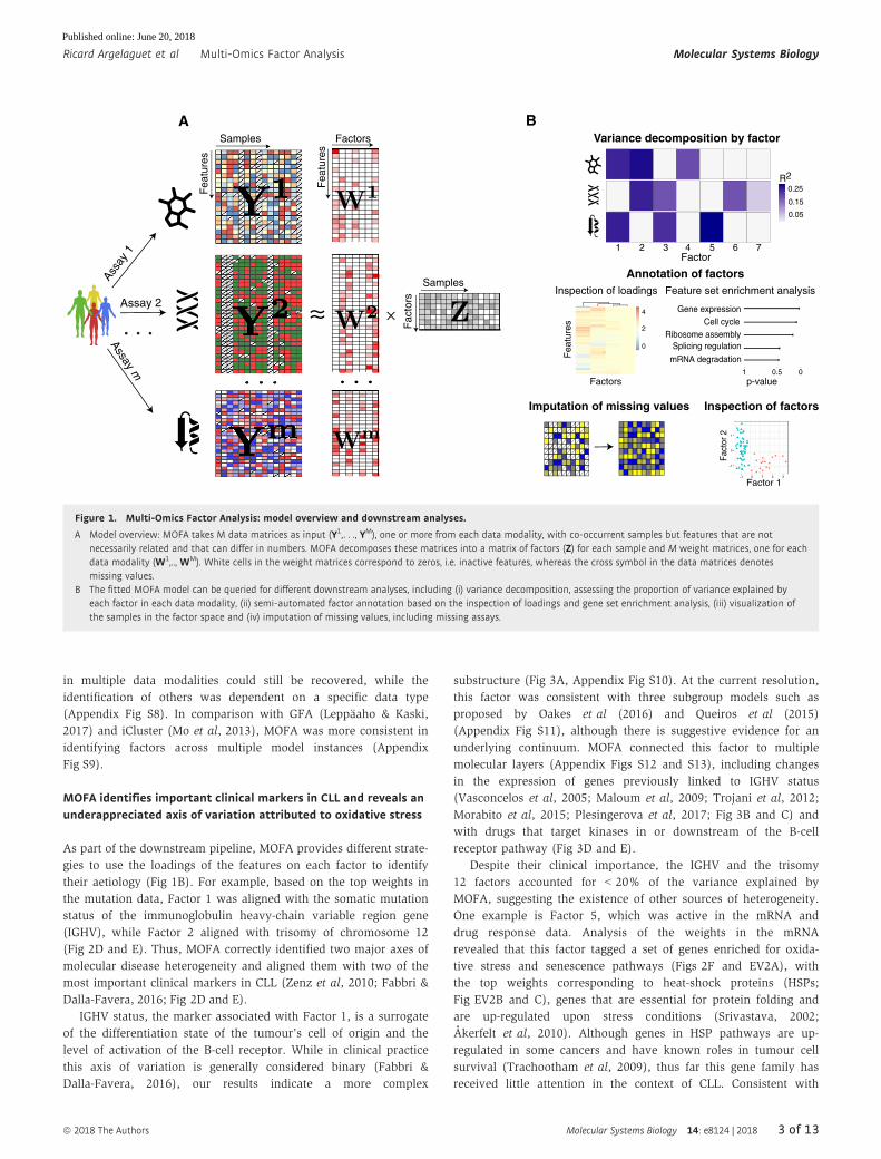
Figure 1. Multi-Omics Factor Analysis: model overview and downstream analyses.

A Model overview: MOFA takes M data matrices as input (Y1,. . ., YM), one or more from each data modality, with co-occurrent samples but features that are notnecessarily related and that can differ in numbers. MOFA decomposes these matrices into a matrix of factors (Z) for each sample and M weight matrices, one for eachdata modality (W1,.., WM). White cells in the weight matrices correspond to zeros, i.e. inactive features, whereas the cross symbol in the data matrices denotesmissing values.

B The fitted MOFA model can be queried for different downstream analyses, including (i) variance decomposition, assessing the proportion of variance explained byeach factor in each data modality, (ii) semi-automated factor annotation based on the inspection of loadings and gene set enrichment analysis, (iii) visualization ofthe samples in the factor space and (iv) imputation of missing values, including missing assays.

ª 2018 The Authors Molecular Systems Biology 14: e8124 | 2018 3 of 13

Ricard Argelaguet et al Multi-Omics Factor Analysis Molecular Systems Biology

Published online: June 20, 2018

this annotation based on the mRNA data, we observed that the

drugs with the strongest weights on Factor 5 were associated with

response to oxidative stress, such as target reactive oxygen species

(ROS), DNA damage response and apoptosis (Fig EV2D and E).

Factor 4 captured 9% of variation in the mRNA data, and gene

set enrichment analysis on the mRNA loadings suggested aetiologies

related to immune response pathways and T-cell receptor signalling

(Fig 2F), likely due to differences in cell type composition between

samples: While the samples are comprised mainly of B cells, Factor

4 revealed a possible contamination with other cell types such as T

cells and monocytes (Appendix Fig S14). Factor 3 explained 11% of

variation in the drug response data capturing differences in the

samples’ general level of drug sensitivity (Geeleher et al, 2016;

Appendix Fig S15).

MOFA identifies outlier samples and accurately imputesmissing values

Next, we explored the relationship between inferred factors and

clinical annotations, which can be missing, mis-annotated or inaccu-

rate, since they are frequently based on single markers or imperfect

surrogates (Westra et al, 2011). Since IGHV status is the major

biomarker impacting on clinical care, we assessed the consistency

between the inferred continuous Factor 1 and this binary marker.

For 176 out of 200 patients, the MOFA factor was in agreement with

the clinical IGHV status, and MOFA further allowed for classifying

12 patients that lacked clinically measured IGHV status (Fig EV3A

and B). Interestingly, MOFA assigned 12 patients to a different

group than suggested by their clinical IGHV label. Upon inspection

1 2 3 4 5 6 7 8 9 10Factor

0.050.100.15

R2

A B

Drugresponse

D=310

MethylationD=4248

mRNAD=5000

MutationsD=69

Patients (N=200)0 0.1 0.2 0.3 0.4

R2

D

N=184

N=196

N=136

N=200

C

gain14q32

del13q14

del14q24.3

del11q22.3

trisomy12

0 0.5 1Absolute loading on Factor 2

BRAF

MED12

del11q22.3

KLHL6

IGHV

0 0.5 1Absolute loading on Factor 1

F RNA regulationImmune Response

cellular stressother

0

20

40

60

80

1 2 3 4 5 6 7 8 9 10Factor

Enr

iche

d ge

ne s

ets

at F

DR

1%

−3

−2

−1

0

1

−1 0 1 2Factor 1

Fact

or 2

U−CLL, no tr12U−CLL, tr12

M−CLL, no tr12M−CLL, tr12 missingE

Figure 2. Application of MOFA to a study of chronic lymphocytic leukaemia.

A Study overview and data types. Data modalities are shown in different rows (D = number of features) and samples (N) in columns, with missing samples shownusing grey bars.

B, C (B) Proportion of total variance explained (R2) by individual factors for each assay and (C) cumulative proportion of total variance explained.D Absolute loadings of the top features of Factors 1 and 2 in the Mutations data.E Visualization of samples using Factors 1 and 2. The colours denote the IGHV status of the tumours; symbol shape and colour tone indicate chromosome 12 trisomy

status.F Number of enriched Reactome gene sets per factor based on the gene expression data (FDR < 1%). The colours denote categories of related pathways defined as in

Appendix Table S2.

4 of 13 Molecular Systems Biology 14: e8124 | 2018 ª 2018 The Authors

Molecular Systems Biology Multi-Omics Factor Analysis Ricard Argelaguet et al

Published online: June 20, 2018

of the underlying molecular data, nine of these cases showed inter-

mediate molecular signatures, suggesting that they are borderline

cases that are not well captured by the binary classification; the

remaining three cases were clearly discordant (Fig EV3C and D).

Additional independent drug response assays as well as whole

exome sequencing data confirmed that these cases are outliers

within their IGHV group (Fig EV3E and F).

As incomplete data is a common problem in studies that combine

multiple high-throughput assays, we assessed the ability of MOFA

to fill in missing values within assays as well as when entire data

modalities are missing for some of the samples. For both imputation

tasks, MOFA yielded more accurate predictions than other estab-

lished imputation strategies, including imputation by feature-wise

mean, SoftImpute (Mazumder et al, 2010) and a k-nearest neigh-

bour method (Troyanskaya et al, 2001; Fig EV4, Appendix Fig S16),

and MOFA was more robust than GFA, especially in the case of

missing assays (Appendix Fig S17).

Latent factors inferred by MOFA are predictive ofclinical outcomes

Finally, we explored the utility of the latent factors inferred by

MOFA as predictors in models of clinical outcomes. Three of the

10 factors identified by MOFA were significantly associated with

time to next treatment (Cox regression, Materials and Methods,

FDR < 1%, Fig 4A and B): Factor 1, related to the B-cell of origin,

Fact

or 1

−1.

5−

0.5

0.5

1.5

Factor clusters

LZ IZ HZ

mRNA

Drugresponse

Concentration [μΜ]

AZD7762 dasatinib

0 10 20 30 40 0 10 20 30 400.00

0.25

0.50

0.75

1.00vi

abili

ty

LZ IZ HZ

NU7441TAE684

thapsigarginMK−1775

ibrutinibSCH 900776

spebrutinibidelalisibduvelisib

PRT062607 HCltamatinib

PF 477736AZD7762AT13387dasatinib

0.0 0.2 0.4 0.6Absolute loading on Factor 1

2468101214

ADAM29WNT9AMAPK4SPG20NETO1BCL7ANPTX1

PSD3RBMS3

PPP1R9AKANK2

CRY1PLD1

L3MBTL4LDOC1

LPLZNF471

SOWAHCSEPT10ZNF667

0.0 0.3 0.6 0.9

ZNF667SEPT10SOWAHCZNF471LPLLDOC1L3MBTL4PLD1CRY1KANK2PPP1R9ARBMS3PSD3NPTX1BCL7ANETO1SPG20MAPK4WNT9AADAM29

Factor 1Clusters

Samples

+−−−−−−−−−−−−−−−−−−−

Drug Categories

BCR pathwayCHKHSP90other

known IGHV-association normalized gene expression

A

B C

ED

Figure 3. Characterization of the inferred factor associated with the differentiation state of the cell of origin.

A Beeswarm plot with Factor 1 values for each sample with colours corresponding to three groups found by 3-means clustering with low factor values (LZ),intermediate factor values (IZ) and high factor values (HZ).

B Absolute loadings for the genes with the largest absolute weights in the mRNA data. Plus or minus symbols on the right indicate the sign of the loading. Geneshighlighted in orange were previously described as prognostic markers in CLL and associated with IGHV status (Vasconcelos et al, 2005; Maloum et al, 2009; Trojaniet al, 2012; Morabito et al, 2015; Plesingerova et al, 2017).

C Heatmap of gene expression values for genes with the largest weights as in (B).D Absolute loadings of the drugs with the largest weights, annotated by target category.E Drug response curves for two of the drugs with top weights, stratified by the clusters as in (A).

ª 2018 The Authors Molecular Systems Biology 14: e8124 | 2018 5 of 13

Ricard Argelaguet et al Multi-Omics Factor Analysis Molecular Systems Biology

Published online: June 20, 2018

and two Factors, 7 and 8, associated with chemo-immunotherapy

treatment prior to sample collection (P < 0.01, t-test). In particular,

Factor 7 captures del17p and TP53 mutations as well as differences

in methylation patterns of oncogenes (Garg et al, 2014; Fluhr et al,

2016; Appendix Fig S18), while Factor 8 is associated with WNT

signalling (Appendix Fig S19).

We also assessed the prediction performance when combining

the 10 MOFA factors in a multivariate Cox regression model.

Notably, this model yielded higher prediction accuracy than models

using components derived from conventional PCA (Fig 4C), individ-

ual molecular features (Appendix Fig S20) or MOFA factors derived

from only a subset of the available data modalities (Appendix Fig

S8B and D; assessed using cross-validation, Materials and Methods).

The predictive value of MOFA factors was similar to clinical covari-

ates (such as lymphocyte doubling time) that are used to guide

treatment decisions (Appendix Fig S21).

+++

+++ ++++++++++++++ ++++ + +++

+

++++++ ++++++++++ ++++++++++ +++ +++++++++++++++

p < 0.00010

25

50

75

100

0 1 2 3Time to treatment

Sur

viva

l pro

babi

lity

(%) Factor 1

+

+

+ ++ + + + +

+

+

+++++++ ++++++++++++++++++++++++++++ +++++++ ++++++++++++++++

p < 0.00010

25

50

75

100

0 1 2 3Time to treatment

Factor 7

++++ ++++ ++ + + + +

+

+++

++++++++ ++++++++++++++++++++++++++++ +++++ +++++++++++++++

p < 0.00010

25

50

75

100

0 1 2 3Time to treatment

Factor 8

A C

B

2.6e−05

0.25

0.11

0.32

0.11

0.95

5.5e−07

3.8e−06

0.094

0.82

0.75 1.00 1.50 2.00 3.00

10

9

8

7

6

5

4

3

2

1

(Positive) Hazard Ratio

Fact

or

0.5

0.6

0.7

0.8

Har

rell'

s C

−in

dex

Met

hyla

tion

MO

FA fa

ctor

s

all

Dru

gs

mR

NA

Mut

atio

ns

Input data

Figure 4. Relationship between clinical data and latent factors.

A Association of MOFA factors to time to next treatment using a univariate Cox regression with N = 174 samples (96 of which are uncensored cases) and P-values basedon the Wald statistic. Error bars denote 95% confidence intervals. Numbers on the right denote P-values for each predictor.

B Kaplan–Meier plots measuring time to next treatment for the individual MOFA factors. The cut-points on each factor were chosen using maximally selected rankstatistics (Hothorn & Lausen, 2003), and P-values were calculated using a log-rank test on the resulting groups.

C Prediction accuracy of time to treatment for N = 174 patients using multivariate Cox regression trained using the 10 factors derived using MOFA, as well using thefirst 10 components obtained from PCA applied to the corresponding single data modalities and the full data set (assessed on hold-out data). Shown are averagevalues of Harrell’s C-index from fivefold cross-validation. Error bars denote standard error of the mean.

6 of 13 Molecular Systems Biology 14: e8124 | 2018 ª 2018 The Authors

Molecular Systems Biology Multi-Omics Factor Analysis Ricard Argelaguet et al

Published online: June 20, 2018

In an application to single cell data MOFA reveals coordinatedchanges between the transcriptome and the epigenome along adifferentiation trajectory

As multi-omics approaches are also beginning to emerge in single-

cell biology (Macaulay et al, 2015; Angermueller et al, 2016; Guo

et al, 2017; Clark et al, 2018; Colome-Tatche & Theis, 2018), we

investigated the potential of MOFA to disentangle the heterogeneity

observed in such studies. We applied MOFA to a data set of 87

mouse embryonic stem cells (mESCs), comprising of 16 cells

cultured in “2i” media, which induces a naive pluripotency state,

and 71 serum-grown cells, which commits cells to a primed

pluripotency state poised for cellular differentiation (Angermueller

et al, 2016). All cells were profiled using single-cell methylation and

transcriptome sequencing, which provides parallel information of

these two molecular layers (Fig 5A). We applied MOFA to disentan-

gle the observed heterogeneity in the transcriptome and the CpG

methylation at three different genomic contexts: promoters, CpG

islands and enhancers.

MOFA identified three major factors driving cell–cell heterogene-

ity (minimum explained variance of 2%, Materials and Methods):

while Factor 1 is shared across all data modalities (7% variance

explained in the RNA data and between 53 and 72% in the methyla-

tion data sets), Factors 2 and 3 are active primarily in the RNA data

Culture

Met CpG IslandsD=5000

Met PromotersD=5000

Met EnhancersD=5000

RNA expressionD=5000

Samples (N=87) 0.0 0.3 0.6

0.0

0.2

0.4

0.6

R2

Factor1 2 3

R2

A B C

D E

−1

0

1

−4 −2 0 2Factor 1

Fac

tor

2

Load

ing

Fac

tor

1Lo

adin

g F

acto

r 2

Klf4Tbx3Tex19.1

Tcl1EsrrbJam2

Fbxo15 Morc1 Zfp42

0.00

0.50

1.00

Rank position

Krt19Anxa3Tagln

AhnakAnxa5Cald1 Krt8

0.00

0.50

1.00

Serum2i

N=81

N=83

N=83

N=83

Figure 5. Application of MOFA to a single-cell multi-omics study.

A Study overview and data types. Data modalities are shown in different rows (D = number of features) and samples (N) in columns, with missing samples shownusing grey bars.

B, C (B) Fraction of the variance explained (R2) by individual factors for each data modality and (C) cumulative proportion of variance explained.D Absolute loadings of Factor 1 (bottom) and Factor 2 (top) in the mRNA data. Labelled genes in Factor 1 are known markers of pluripotency (Mohammed et al, 2017)

and genes labelled in Factor 2 are known differentiation markers (Fuchs, 1988).E Scatterplot of Factors 1 and 2. Colours denote culture conditions. The grey arrow illustrates the differentiation trajectory from naive pluripotent cells via primed

pluripotent cells to differentiated cells.

ª 2018 The Authors Molecular Systems Biology 14: e8124 | 2018 7 of 13

Ricard Argelaguet et al Multi-Omics Factor Analysis Molecular Systems Biology

Published online: June 20, 2018

(Fig 5B and C). Gene loadings revealed that Factor 1 captured the

cells’ transition from naıve to primed pluripotent states, pinpointing

pluripotency markers such as Rex1/Zpf42, Tbx3, Fbxo15 and Essrb

(Mohammed et al, 2017; Figs 5D and EV5A). MOFA connected

these transcriptomic changes to coordinated changes in the genome-

wide DNA methylation rate across all genomic contexts (Fig EV5B),

as previously described both in vitro (Angermueller et al, 2016) and

in vivo (Auclair et al, 2014). Factor 2 captured a second axis of dif-

ferentiation from the primed pluripotency state to a differentiated

state with highest RNA loadings for known differentiation markers

such as keratins and annexins (Fuchs, 1988; Figs 5D and EV5C).

Finally, Factor 3 captured the cellular detection rate, a known tech-

nical covariate associated with cell quality and mRNA content

(Finak et al, 2015; Appendix Fig S22).

Jointly, Factors 1 and 2 captured the entire differentiation trajec-

tory from naive pluripotent cells via primed pluripotent cells to dif-

ferentiated cells (Fig 5E), illustrating the importance of learning

continuous latent factors rather than discrete sample assignments.

Multi-omics clustering algorithms such as SNF (Wang et al, 2014)

or iCluster (Shen et al, 2009; Mo et al, 2013) were only capable of

distinguishing cellular subpopulations, but not of recovering contin-

uous processes such as cell differentiation (Appendix Fig S23).

Discussion

Multi-Omics Factor Analysis (MOFA) is an unsupervised method for

decomposing the sources of heterogeneity in multi-omics data sets.

We applied MOFA to high-dimensional and incomplete multi-omics

profiles collected from patient-derived tumour samples and to a

single-cell study of mESCs.

First, in the CLL study, we demonstrated that our method is able

to identify major drivers of variation in a clinically and biologically

heterogeneous disease. Most notably, our model identified previ-

ously known clinical markers as well as novel putative molecular

drivers of heterogeneity, some of which were predictive of clinical

outcome. Additionally, since MOFA factors capture variations of

multiple features and data modalities, inferred factors can help to

mitigate assay noise, thereby increasing the sensitivity for identify-

ing molecular signatures compared to using individual features or

assays. Our results also demonstrate that MOFA can leverage infor-

mation from multiple omics layers to accurately impute missing

values from sparse profiling data sets and guide the detection of

outliers, e.g. due to mislabelled samples or sample swaps.

In a second application, we used MOFA for the analysis of single-

cell multi-omics data. This use case illustrates the advantage of

learning continuous factors, rather than discrete groups, enabling

MOFA to recover a differentiation trajectory by combining informa-

tion from two sparsely profiled molecular layers.

While applications of factor models for integrating different data

types were reported previously (Lanckriet et al, 2004; Shen et al,

2009; Akavia et al, 2010; Mo et al, 2013), MOFA provides unique

features (Materials and Methods, Appendix Table S3) that enable

the interpretable reconstruction of the underlying factors and

accommodating different data types as well as different patterns of

missing data. MOFA is available as open-source software and

includes semi-automated analysis pipelines allowing for in-depth

characterizations of inferred factors. Taken together, this will foster

the accessibility of interpretable factor models for a wide range of

multi-omics studies.

Although we have addressed important challenges for multi-

omics applications, MOFA is not free of limitations. The model is

linear, which means that it can miss strongly non-linear relation-

ships between features within and across assays (Buettner & Theis,

2012). Non-linear extensions of MOFA may address this, although,

as with any models in high-dimensional spaces, there will be trade-

offs between model complexity, computational efficiency and inter-

pretability (preprint: Damianou et al, 2016). A related area of work

is to incorporate prior information on the relationships between

individual features. For example, future extensions could make use

of pathway databases within each omic type (Buettner et al, 2017)

or priors that reflect relationships given by the “dogma of molecular

biology”. In addition, new likelihoods and noise models could

expand the value of MOFA in data sets with specific statistical prop-

erties that hamper the application of traditional statistical methods,

including zero-inflated data (i.e. scRNA-Seq; Pierson & Yau, 2015)

or binomial distributed data (i.e. splicing events; Huang & Sangui-

netti, 2017). Finally, while here we focus our attention on the point

estimates of inferred factors, future extensions could attempt a more

comprehensive Bayesian treatment that propagates evidence

strength and estimation uncertainties to diagnostics and down-

stream analyses.

Materials and Methods

Multi-Omics Factor Analysis model

Starting from M data matrices Y1,..,YM of dimensions N × Dm,

where N is the number of samples and Dm the number of features in

data matrix m, MOFA decomposes these matrices as

Ym ¼ ZWmT þ em m ¼ 1; . . .;M: (1)

Here, Z denotes the factor matrix (common for all data matrices)

and Wm denotes the weight matrices for each data matrix m (also

referred to as view m in the following). em denotes the view-

specific residual noise term, with its form depending on the speci-

fics of the data type (see Noise model).

The model is formulated in a probabilistic Bayesian framework,

where we place prior distributions on all unobserved variables of

the model (see plate diagram in Appendix Fig S24), i.e. the factors

Z, the weight matrices Wm and the parameters of the residual noise

term. In particular, we use a standard normal prior for the factors Z

and employ sparsity priors for the weight matrices (see next

section).

Model regularization

An appropriate regularization of the weight matrices is essential for

the model’s ability to disentangle variation across data sets and to

yield interpretable factors. MOFA uses a two-level regularization:

the first level encourages view- and factor-wise sparsity, thereby

allowing to directly identify which factor is active in which view.

The second level encourages feature-wise sparsity, thereby typically

resulting in a small number of features with active weights. To

8 of 13 Molecular Systems Biology 14: e8124 | 2018 ª 2018 The Authors

Molecular Systems Biology Multi-Omics Factor Analysis Ricard Argelaguet et al

Published online: June 20, 2018

encode these sparsity levels, we combine an Automatic Relevance

Determination (ARD) prior for the first type of the sparsity with a

spike-and-slab prior for the second. For amenable inference, we

model the spike-and-slab prior by parameterizing the weights as a

product of a Bernoulli distributed random variable and a normally

distributed random variable: W ¼ ScW , where smdk � Ber ðhmk Þ andcWmdk � Nð0; 1=amk Þ. To automatically learn the appropriate level of

regularization for each factor and view, we use uninformative

conjugate prior on amk , which controls the strength of factor k in

view m, and on hmk , which determines the feature-wise sparsity level

of factor k in view m (see Appendix Supplementary Methods,

Section 2 for details).

Noise model

MOFA supports the combination of different noise models to inte-

grate diverse data types, including continuous, binary and count

data. A standard noise model for continuous data is the Gaussian

noise model assuming iid heteroscedastic residuals em, i.e.

emnd � Nð0; 1=smd Þ, with Gamma prior on the precision parameters smd .MOFA further supports noise models for binary and count data that

are not appropriately modelled using a Gaussian likelihood. In the

current version, MOFA models count data using a Poisson model

and binary data by using a Bernoulli model. Here, the model likeli-

hood is given by ymnd � Poi k Zn:wTd:

� �� �and ymnd � Ber r Zn:w

Td:

� �� �,

respectively, where kðxÞ ¼ logð1 þ exÞ and r denotes the logistic

function rðxÞ ¼ ð1 þ e�xÞ�1.

Parameter inference

For scalability, we make use of a variational Bayesian framework,

which is essentially a mean field approximation for approximate

inference (Blei et al, 2017). The key idea is to approximate the

intractable posterior distribution using a simpler class of distribu-

tions by minimizing the Kullback–Leibler divergence to the exact

posterior, or equivalently maximizing the evidence lower bound

(ELBO). Convergence of the algorithm can be monitored based on

the ELBO. An overview of variational inference and details on the

specific implementation for MOFA can be found in Appendix Supple-

mentary Methods, Section 3. To enable an efficient inference for

non-Gaussian likelihoods, we employ variational lower bounds on

the likelihood (Jaakkola & Jordan, 2000; Seeger & Bouchard, 2012;

see Appendix Supplementary Methods, Section 4).

Model training and selection

An important part of the training is the determination of the number

of factors. Factors are automatically inactivated by the ARD prior of

the model as described in Model regularization. In practice, factors

are pruned during training using a minimum fraction of variance

explained threshold that needs to be specified by the user. Alterna-

tively, the user can fix the number of factors and the minimum vari-

ance criterion is ignored. In the analyses presented, we initialized

the models with K = 25 factors and they were pruned during train-

ing using a threshold of variance explained of 2%. For details on the

implementation as well as practical considerations for training and

choice of the threshold parameter, refer to Appendix Supplementary

Methods, Section 5.

While the inferred factors are robust under different initializa-

tions (e.g. Appendix Fig S6C and D), the optimization landscape is

non-convex, and hence, the algorithm is not guaranteed to converge

to a global optimum. Results presented here are based on 10–25

random restarts, selecting the model with the highest ELBO (e.g.

Appendix Fig S6B).

Downstream analysis for factor interpretation and annotation

As part of MOFA, we provide the R package MOFAtools, which

provides a semi-automated pipeline for the characterization and

interpretation of the latent factors. In all downstream analyses, we

use the expectations of the model variables under the posterior

distributions inferred by the variational framework.

The first step, after a model has been trained, is to disentangle

the variation explained by each factor in each view. To this end, we

compute the fraction of the variance explained (R2) by factor k in

view m as

R2m;k ¼ 1�

Xn;d

ymnd � znkwmkd � lmd

� �2=

Xn;d

ymnd � lmd

� �2

as well as the fraction of variance explained per view taking into

account all factors

R2m ¼ 1�

Xn;d

ymnd �X

kznkw

mkd � lmd

� �2=

Xn;d

ymnd � lmd

� �2

Here, lmd denotes the feature-wise mean. Subsequently, each

factor is characterized by three complementary analyses:

1 Ordination of the samples in factor space: Visualize a low-

dimensional representation of the main drivers of sample

heterogeneity.

2 Inspection of top features with largest weight: The loadings can

give insights into the biological process underlying the hetero-

geneity captured by a latent factor. Due to scale differences

between assays, the weights of different views are not directly

comparable. For simplicity, we scale each weight vector by its

absolute value.

3 Feature set enrichment analysis: Combine the signal from func-

tionally related sets of features (e.g. gene sets) to derive a

feature set-based annotation. By default, we use a parametric

t-test comparing the means of the foreground set (the weights

of features that belong to a set G) and the background set (the

weights of features that do not belong to the set G), similar to

the approach described in Frost et al (2015).

Relationship to existing methods

MOFA builds upon the statistical framework of group Factor

Analysis (Virtanen et al, 2012; Khan et al, 2014; Klami et al, 2015;

Bunte et al, 2016; Zhao et al, 2016; Leppaaho & Kaski, 2017) and is

in part also related to the iCluster methods (Shen et al, 2009; Mo

et al, 2013) as shown in Appendix Table S3. Here, we describe these

connections in further detail.

iCluster

In contrast to MOFA, iCluster uses in each view the same extent of

regularization for all factors, which may be sufficient for the

purpose of clustering (the primary application of iCluster); however,

ª 2018 The Authors Molecular Systems Biology 14: e8124 | 2018 9 of 13

Ricard Argelaguet et al Multi-Omics Factor Analysis Molecular Systems Biology

Published online: June 20, 2018

it results in a reduced ability for distinguishing factors that drive

variation in distinct subsets of views (Appendix Fig S5). Addition-

ally, unlike MOFA and GFA, iCluster does not handle missing values

and is computationally demanding (Fig EV1), as it requires re-fitting

the model for a large range of different penalty parameters and

choices of the model dimension.

Group Factor Analysis

While the underlying model of MOFA is closely connected to the

most recent GFA implementation (Leppaaho & Kaski, 2017), GFA

is restricted to Gaussian observation noise. In terms of the algo-

rithmic implementation, MOFA uses an additional “burn-in period”

during training during which the sparsity constraints are deacti-

vated to avoid early splitting of factors and actively drops factors

below a predefined variance threshold (see Model training and

selection). In contrast, GFA directly uses sparsity constraints

throughout training and also maintains factors that have near-zero

relevance. In terms of inference, MOFA is implemented using a

variational approximate Bayesian inference, whereas GFA is based

on a Gibbs sampler. In terms of computational scalability

(Fig EV1), both methods are linear in the model’s parameters,

although GFA is computationally more expensive in absolute

terms. This difference is particularly pronounced for data sets with

missing data. This, together with the inability to deactivate factors

during inference (Appendix Fig S4), renders GFA considerably

slower in applications to real data.

Details on the simulation studies

Model validation

To validate MOFA, we simulated data from the generative model

for a varying number of views (M = 1,3,. . .,21), features

(D = 100,500,. . .,10,000), factors (K = 5,10,. . .,60), missing values

(from 0 to 90%) as well as for non-Gaussian likelihoods (Poisson,

Bernoulli; see Appendix Table S1 for simulation parameters). We

assessed the ability of MOFA to recover the true simulated number

of factors in the different settings, where we considered 10 repeat

experiments for every configuration. All trials were started with a

high number of factors (K = 100), and inactive factors were pruned

as described in Model training and selection.

Model comparison

To compare MOFA with to GFA, we simulated data from the

underlying generative model with Ktrue = 10 factors, M = 3 views,

N = 100 samples, D = 5,000 features each and 5% missing values

(missing at random). For each of the three views, we used a dif-

ferent likelihood model: continuous data were simulated with a

Gaussian distribution, binary data with a Bernoulli distribution

and count data with a Poisson distribution. Except for the non-

Gaussian likelihood extension, both methods share the same

underlying generative model, thus allowing for a meaningful

comparison. We fit ten realizations of the MOFA and GFA models

with Kinitial = 20 factors and let the method determine the most

likely number factors. To assess scalability, we considered the

same base parameter settings, varying one of the simulation

parameters at a time (number of factors K, number of features D,

number of samples N and number of views M, all Gaussian). To

assess the ability to reconstruct factor activity patterns, we

simulated data from the generative model for Ktrue = 10 and

Ktrue = 15 factors (M, N, D as before, no missing values, only

Gaussian views), where factors were set to either active or inactive

in a specific view by sampling the parameter amk from {1,103}.

Appendix Table S1 shows in more detail the simulation parameters

used in each setting.

Details on the CLL analysis

Data processing

The data were taken from (Dietrich et al, 2018), where details on

the data generation and processing can be found. Briefly, this data

set consists of somatic mutations (combination of targeted and

whole exome sequencing), RNA expression (RNA-Seq), DNA methy-

lation (Illumina arrays) and ex vivo drug response screens (ATP-

based CellTiter-Glo assay). For the training of MOFA, we included

62 drug response measurements (excluding NSC 74859 and borte-

zomib due to bad quality) at five concentrations each (D = 310)

with a threshold at 1.1 to remove outliers. Mutations were consid-

ered if present in at least three samples (D = 69). Low counts from

RNA-Seq data were filtered out and the data were normalized using

the estimateSizeFactors and varianceStabilizingTransformation func-

tion of DESeq2 (Love et al, 2014). For training, we considered the

top D = 5,000 most variable mRNAs after exclusion of genes from

the Y chromosome. Methylation data were transformed to M-values,

and we extracted the top 1% most variable CpG sites excluding sex

chromosomes (D = 4,248). We included patients diagnosed with

CLL and having data in at least two views into the MOFA model

leading to a total of N = 200 samples.

Model training and selection

We trained MOFA using 25 random initializations with a variance

threshold of 2% and selected the model with the best fit for down-

stream analysis (see Model training and selection).

Gene set enrichment analysis

Gene set enrichment analysis was performed based on Reactome

gene sets (Fabregat et al, 2015) as described above. Resulting P-

values were adjusted for multiple testing for each factor using the

Benjamini–Hochberg procedure (Benjamini & Hochberg, 1995).

Significant enrichments were at a false discovery rate of 1%.

Imputation

To compare imputation performance, we trained MOFA on the

subset of samples with all measurements (N = 121) and masked at

random either single values or all measurements for randomly

selected samples in the drug response. After model training, the

masked values were imputed directly from the model equation (1)

and the accuracy was assessed in terms of mean squared error on

the true (masked) values. For both settings, we fixed the number of

factors in MOFA to K = 10. To investigate the dependence on K for

imputation and to compare MOFA to GFA, we re-ran the same

masking experiments varying K = 1,. . .,20 (Appendix Fig S17).

Survival analysis

Associations between the inferred factors and clinical covariates

were assessed using the patients’ time to next treatment as

10 of 13 Molecular Systems Biology 14: e8124 | 2018 ª 2018 The Authors

Molecular Systems Biology Multi-Omics Factor Analysis Ricard Argelaguet et al

Published online: June 20, 2018

response variable in a Cox model (N = 174 samples with treatment

information, 96 of which are uncensored cases). For univariate

association tests (as shown in Fig 4A, Appendix Fig S21), we

scaled all predictors to ensure comparability of the hazard ratios

and we rotated factors, which are rotational invariant, such that

their hazard ratio is greater or equal to 1. To investigate the

predictive power of different data sets, we used a multivariate Cox

model and compared Harrell’s C-index of predictions in a stratified

fivefold cross-validation scheme. As predictors, we included the

top 10 principal components calculated on the data for each single

view, a concatenated data set (“all”) as well as the 10 MOFA

factors. Missing values in a view were set to the feature-wise

mean. In a second set of models, we used the complete set of all

features in a view with a ridge penalty in the Cox model as imple-

mented in the R package glmnet. For the Kaplan–Meier plots, an

optimal cut-point on each factor was determined to define the two

groups using the maximally selected rank statistics as implemented

in the R package survminer with P-values based on a log-rank test

between the resulting groups.

Details on the scMT analysis

The data were obtained from Angermueller et al (2016), where

details on the data generation and pre-processing can be found.

Briefly for each CpG site, we calculated a binary methylation rate

from the ratio of methylated read counts to total read counts. RNA

expression data were normalized using Lun et al (2016). To fit

MOFA, we considered the top 5,000 most variable genes with a

maximum dropout of 90% and the top 5,000 most variable CpG

sites with a minimum coverage of 10% across cells. Model selection

was performed as described for the CLL data, and factors were inac-

tivated below a minimum explained variance of 2%. For the cluster-

ing analysis using SNF and iCluster, the optimal number of clusters

was selected using the BIC criterion.

Data and software availability

• The CLL data were obtained from Dietrich et al (2018) and

are available at the European Genome–Phenome Archive under

accession EGAS00001001746 and data tables as R objects can be

downloaded from http://pace.embl.de/. The single-cell data were

obtained from Angermueller et al (2016) and are available in the

Gene Expression Omnibus under accession GSE74535. All data

used are contained within the MOFA vignettes and can be down-

loaded as from https://github.com/bioFAM/MOFA.

• An open-source implementation of MOFA in R and Python is

available from https://github.com/bioFAM/MOFA. Code to repro-

duce all the analyses presented is available at https://github.com/

bioFAM/MOFA_analysis.

Expanded View for this article is available online.

AcknowledgementsWe thank everybody involved in the generation and analysis of the original

CLL study for sharing their data and analysis ahead of publication, especially

M. Ole�s for providing the associated data package and to J. Lu, J. Hüllein and A.

Mock for discussions on CLL biology. The work was supported by the European

Union (Horizon 2020 project SOUND) and project PanCanRisk).

Author contributionsRA and BV contributed equally and are listed alphabetically. FB, DA and OS

conceived the model. RA, DA and BV implemented the model. TZ, SD and WH

designed the CLL study and generated the data. RA and BV performed the

analysis. RA, BV, DA, TZ, SD, WH, OS, FB and JCM interpreted the results. RA, BV,

OS, WH and FB conceived the project. RA, BV, OS, FB and WH wrote the manu-

script. OS, WH, FB and JCM supervised the project.

Conflict of interestThe authors declare that they have no conflict of interest.

ReferencesAkavia UD, Litvin O, Kim J, Sanchez-Garcia F, Kotliar D, Causton HC,

Pochanard P, Mozes E, Garraway LA, Pe’er D (2010) An integrated

approach to uncover drivers of cancer. Cell 143: 1005 – 1017

Åkerfelt M, Morimoto RI, Sistonen L (2010) Heat shock factors: integrators of

cell stress, development and lifespan. Nat Rev Mol Cell Biol 11: 545

Angermueller C, Clark SJ, Lee HJ, Macaulay IC, Teng MJ, Hu TX, Krueger F,

Smallwood S, Ponting CP, Voet T, Kelsey G, Stegle O, Reik W (2016)

Parallel single-cell sequencing links transcriptional and epigenetic

heterogeneity. Nat Methods 13: 229 – 232

Auclair G, Guibert S, Bender A, Weber M (2014) Ontogeny of CpG island

methylation and specificity of DNMT3 methyltransferases during

embryonic development in the mouse. Genome Biol 15: 545

Benjamini Y, Hochberg Y (1995) Controlling the false discovery rate: a

practical and powerful approach to multiple testing. J R Stat Soc B 57:

289 – 300

Blei DM, Kucukelbir A, McAuliffe JD (2017) Variational inference: a review for

statisticians. J Am Stat Assoc 112: 859 – 877

Buettner F, Theis FJ (2012) A novel approach for resolving differences in

single-cell gene expression patterns from zygote to blastocyst.

Bioinformatics 28: i626 – i632

Buettner F, Pratanwanich N, McCarthy DJ, Marioni JC, Stegle O (2017) f-

scLVM: scalable and versatile factor analysis for single-cell RNA-seq.

Genome Biol 18: 212

Bunte K, Leppaaho E, Saarinen I, Kaski S (2016) Sparse group factor

analysis for biclustering of multiple data sources. Bioinformatics 32:

2457 – 2463

Cancer Genome Atlas Research Network (2017) Comprehensive and

integrative genomic characterization of hepatocellular carcinoma. Cell 169:

1327 – 1341.e1323

Chen L, Ge B, Casale FP, Vasquez L, Kwan T, Garrido-Martín D, Watt S, Yan Y,

Kundu K, Ecker S (2016) Genetic drivers of epigenetic and transcriptional

variation in human immune cells. Cell 167: 1398 – 1414.e1324

Clark SJ, Argelaguet R, Kapourani C-A, Stubbs TM, Lee HJ, Alda-Catalinas C,

Krueger F, Sanguinetti G, Kelsey G, Marioni JC (2018) scNMT-seq enables

joint profiling of chromatin accessibility DNA methylation and

transcription in single cells. Nat Commun 9: 781

Colomé-Tatché M, Theis F (2018) Statistical single cell multi-omics

integration. Curr Opin Syst Biol 7: 54 – 59

Damianou A, Lawrence ND, Ek CH (2016) Multi-view learning as a

nonparametric nonlinear inter-battery factor analysis. arXiv 1604.04939.

https://arxiv.org/abs/1604.04939 [PREPRINT]

Dietrich S, Ole�s M, Lu J, Sellner L, Anders S, Velten B, Wu B, Hüllein J, da Silva

Liberio M, Walther T (2018) Drug-perturbation-based stratification of

blood cancer. J Clin Invest 128: 427 – 445

Fabbri G, Dalla-Favera R (2016) The molecular pathogenesis of chronic

lymphocytic leukaemia. Nat Rev Cancer 16: 145 – 162

ª 2018 The Authors Molecular Systems Biology 14: e8124 | 2018 11 of 13

Ricard Argelaguet et al Multi-Omics Factor Analysis Molecular Systems Biology

Published online: June 20, 2018

Fabregat A, Sidiropoulos K, Garapati P, Gillespie M, Hausmann K, Haw R,

Jassal B, Jupe S, Korninger F, McKay S (2015) The reactome pathway

knowledgebase. Nucleic Acids Res 44: D481 –D487

Finak G, McDavid A, Yajima M, Deng J, Gersuk V, Shalek AK, Slichter CK, Miller

HW, McElrath MJ, Prlic M (2015) MAST: a flexible statistical framework for

assessing transcriptional changes and characterizing heterogeneity in

single-cell RNA sequencing data. Genome Biol 16: 278

Fluhr S, Boerries M, Busch H, Symeonidi A, Witte T, Lipka DB, Mücke O,

Nöllke P, Krombholz CF, Niemeyer CM (2016) CREBBP is a target of

epigenetic, but not genetic, modification in juvenile myelomonocytic

leukemia. Clin Epigenet 8: 50

Frost HR, Li Z, Moore JH (2015) Principal component gene set enrichment

(PCGSE). BioData Min 8: 25

Fuchs E (1988) Keratins as biochemical markers of epithelial differentiation.

Trends Genet 4: 277 – 281

Garg R, Benedetti LG, Abera MB, Wang H, Abba M, Kazanietz MG (2014)

Protein kinase C and cancer: what we know and what we do not.

Oncogene 33: 5225 – 5237

Geeleher P, Cox NJ, Huang RS (2016) Cancer biomarker discovery is improved

by accounting for variability in general levels of drug sensitivity in pre-

clinical models. Genome Biol 17: 190

Gerstung M, Pellagatti A, Malcovati L, Giagounidis A, Porta MG, Jadersten M,

Dolatshad H, Verma A, Cross NC, Vyas P, Killick S, Hellstrom-Lindberg E,

Cazzola M, Papaemmanuil E, Campbell PJ, Boultwood J (2015) Combining

gene mutation with gene expression data improves outcome prediction in

myelodysplastic syndromes. Nat Commun 6: 5901

GTEx Consortium (2015) The genotype-tissue expression (GTEx) pilot analysis:

multitissue gene regulation in humans. Science 348: 648 – 660

Guo F, Li L, Li J, Wu X, Hu B, Zhu P, Wen L, Tang F (2017) Single-cell multi-

omics sequencing of mouse early embryos and embryonic stem cells. Cell

Res 27: 967 – 988

Hasin Y, Seldin M, Lusis A (2017) Multi-omics approaches to disease. Genome

Biol 18: 83

Hore V, Viñuela A, Buil A, Knight J, McCarthy MI, Small K, Marchini J (2016)

Tensor decomposition for multiple-tissue gene expression experiments.

Nat Genet 48: 1094 – 1100

Hothorn T, Lausen B (2003) On the exact distribution of maximally selected

rank statistics. Comput Stat Data Anal 43: 121 – 137

Huang Y, Sanguinetti G (2017) BRIE: transcriptome-wide splicing

quantification in single cells. Genome Biol 18: 123

Iorio F, Knijnenburg TA, Vis DJ, Bignell GR, Menden MP, Schubert M, Aben N,

Goncalves E, Barthorpe S, Lightfoot H, Cokelaer T, Greninger P, van Dyk E,

Chang H, de Silva H, Heyn H, Deng X, Egan RK, Liu Q, Mironenko T et al

(2016) A landscape of pharmacogenomic interactions in cancer. Cell 166:

740 – 754

Jaakkola TS, Jordan MI (2000) Bayesian parameter estimation via variational

methods. Stat Comput 10: 25 – 37

Khan SA, Virtanen S, Kallioniemi OP, Wennerberg K, Poso A, Kaski S (2014)

Identification of structural features in chemicals associated with cancer

drug response: a systematic data-driven analysis. Bioinformatics 30:

i497 – i504

Kim M, Rai N, Zorraquino V, Tagkopoulos I (2016) Multi-omics integration

accurately predicts cellular state in unexplored conditions for Escherichia

coli. Nat Commun 7: 13090

Klami A, Virtanen S, Leppaaho E, Kaski S (2015) Group factor analysis. IEEE

Trans Neural Netw Learn Syst 26: 2136 – 2147

Lanckriet GR, De Bie T, Cristianini N, Jordan MI, Noble WS (2004) A statistical

framework for genomic data fusion. Bioinformatics 20: 2626 – 2635

Leppäaho E, Kaski S (2017) GFA: exploratory analysis of multiple data sources

with group factor analysis. J Mach Learn Res 18: 1 – 5

Love MI, Huber W, Anders S (2014) Moderated estimation of fold change and

dispersion for RNA-seq data with DESeq2. Genome Biol 15: 550

Lun AT, Bach K, Marioni JC (2016) Pooling across cells to normalize single-cell

RNA sequencing data with many zero counts. Genome Biol 17: 75

Macaulay IC, Haerty W, Kumar P, Li YI, Hu TX, Teng MJ, Goolam M, Saurat N,

Coupland P, Shirley LM, Smith M, Van der Aa N, Banerjee R, Ellis PD, Quail

MA, Swerdlow HP, Zernicka-Goetz M, Livesey FJ, Ponting CP, Voet T (2015)

G&T-seq: parallel sequencing of single-cell genomes and transcriptomes.

Nat Methods 12: 519 – 522

Maloum K, Settegrana C, Chapiro E, Cazin B, Lepretre S, Delmer A, Leporrier

M, Dreyfus B, Tournilhac O, Mahe B, Nguyen-Khac F, Lesty C, Davi F,

Merle-Beral H (2009) IGHV gene mutational status and LPL/ADAM29 gene

expression as clinical outcome predictors in CLL patients in remission

following treatment with oral fludarabine plus cyclophosphamide. Ann

Hematol 88: 1215 – 1221

Mazumder R, Hastie T, Tibshirani R (2010) Spectral regularization algorithms

for learning large incomplete matrices. J Mach Learn Res 11: 2287 – 2322

Meng C, Kuster B, Culhane AC, Gholami AM (2014) A multivariate approach

to the integration of multi-omics datasets. BMC Bioinformatics 15: 162

Meng C, Zeleznik OA, Thallinger GG, Kuster B, Gholami AM, Culhane AC

(2016) Dimension reduction techniques for the integrative analysis of

multi-omics data. Brief Bioinform 17: 628 – 641

Mertins P, Mani DR, Ruggles KV, Gillette MA, Clauser KR, Wang P, Wang X,

Qiao JW, Cao S, Petralia F, Kawaler E, Mundt F, Krug K, Tu Z, Lei JT, Gatza

ML, Wilkerson M, Perou CM, Yellapantula V, Huang KL et al (2016)

Proteogenomics connects somatic mutations to signalling in breast

cancer. Nature 534: 55 – 62

Mo Q, Wang S, Seshan VE, Olshen AB, Schultz N, Sander C, Powers RS,

Ladanyi M, Shen R (2013) Pattern discovery and cancer gene identification

in integrated cancer genomic data. Proc Natl Acad Sci USA 110:

4245 – 4250

Mohammed H, Hernando-Herraez I, Savino A, Scialdone A, Macaulay I, Mulas

C, Chandra T, Voet T, Dean W, Nichols J (2017) Single-cell landscape of

transcriptional heterogeneity and cell fate decisions during mouse early

gastrulation. Cell Rep 20: 1215 – 1228

Morabito F, Cutrona G, Mosca L, D’Anca M, Matis S, Gentile M, Vigna E,

Colombo M, Recchia AG, Bossio S, De Stefano L, Maura F, Manzoni M,

Ilariucci F, Consoli U, Vincelli I, Musolino C, Cortelezzi A, Molica S,

Ferrarini M et al (2015) Surrogate molecular markers for IGHV mutational

status in chronic lymphocytic leukemia for predicting time to first

treatment. Leuk Res 39: 840 – 845

Oakes CC, Seifert M, Assenov Y, Gu L, Przekopowitz M, Ruppert AS, Wang Q,

Imbusch CD, Serva A, Koser SD, Brocks D, Lipka DB, Bogatyrova O,

Weichenhan D, Brors B, Rassenti L, Kipps TJ, Mertens D, Zapatka M,

Lichter P et al (2016) DNA methylation dynamics during B cell maturation

underlie a continuum of disease phenotypes in chronic lymphocytic

leukemia. Nat Genet 48: 253 – 264

Pierson E, Yau C (2015) ZIFA: dimensionality reduction for zero-inflated

single-cell gene expression analysis. Genome Biol 16: 241

Plesingerova H, Librova Z, Plevova K, Libra A, Tichy B, Skuhrova Francova H,

Vrbacky F, Smolej L, Mayer J, Bryja V, Doubek M, Pospisilova S (2017)

COBLL1, LPL and ZAP70 expression defines prognostic subgroups of

chronic lymphocytic leukemia patients with high accuracy and correlates

with IGHV mutational status. Leuk Lymphoma 58: 70 – 79

Queiros AC, Villamor N, Clot G, Martinez-Trillos A, Kulis M, Navarro A, Penas EM,

Jayne S, Majid A, Richter J, Bergmann AK, Kolarova J, Royo C, Russinol N,

12 of 13 Molecular Systems Biology 14: e8124 | 2018 ª 2018 The Authors

Molecular Systems Biology Multi-Omics Factor Analysis Ricard Argelaguet et al

Published online: June 20, 2018

Castellano G, Pinyol M, Bea S, Salaverria I, Lopez-Guerra M, Colomer D et al

(2015) A B-cell epigenetic signature defines three biologic subgroups of

chronic lymphocytic leukemia with clinical impact. Leukemia 29: 598 – 605

Remes S, Mononen T, Kaski S (2015) Classification of weak multi-view signals

by sharing factors in a mixture of Bayesian group factor analyzers. arXiv

1512.05610. https://arxiv.org/abs/1512.05610 [PREPRINT]

Ritchie MD, Holzinger ER, Li R, Pendergrass SA, Kim D (2015) Methods of

integrating data to uncover genotype-phenotype interactions. Nat Rev

Genet 16: 85 – 97

Seeger M, Bouchard G (2012) Fast variational Bayesian inference for

non-conjugate matrix factorization models. Artific Intell Stat 22: 1012 – 1018

Shen R, Olshen AB, Ladanyi M (2009) Integrative clustering of multiple

genomic data types using a joint latent variable model with application

to breast and lung cancer subtype analysis. Bioinformatics 25: 2906 – 2912

Singh A, Gautier B, Shannon CP, Rohart F, Vacher M, Tebutt SJ, Le Cao K-A

(2018) DIABLO: from multi-omics assays to biomarker discovery, an

integrative approach. bioRxiv https://doi.org/10.1101/067611 [PREPRINT]

Soderholm S, Fu Y, Gaelings L, Belanov S, Yetukuri L, Berlinkov M, Cheltsov

AV, Anders S, Aittokallio T, Nyman TA, Matikainen S, Kainov DE (2016)

Multi-omics studies towards novel modulators of influenza A virus-host

interaction. Viruses 8: 269

Srivastava P (2002) Roles of heat-shock proteins in innate and adaptive

immunity. Nat Rev Immunol 2: 185

Tenenhaus A, Philippe C, Guillemot V, Le Cao K-A, Grill J, Frouin V (2014)

Variable selection for generalized canonical correlation analysis.

Biostatistics 15: 569 – 583

Trachootham D, Alexandre J, Huang P (2009) Targeting cancer cells by ROS-

mediated mechanisms: a radical therapeutic approach? Nat Rev Drug

Discovery 8: 579 – 591

Trojani A, Di Camillo B, Tedeschi A, Lodola M, Montesano S, Ricci F, Vismara

E, Greco A, Veronese S, Orlacchio A (2012) Gene expression profiling

identifies ARSD as a new marker of disease progression and the

sphingolipid metabolism as a potential novel metabolism in chronic

lymphocytic leukemia. Cancer Biomarkers 11: 15 – 28

Troyanskaya O, Cantor M, Sherlock G, Brown P, Hastie T, Tibshirani R,

Botstein D, Altman RB (2001) Missing value estimation methods for DNA

microarrays. Bioinformatics 17: 520 – 525

Vasconcelos Y, De Vos J, Vallat L, Reme T, Lalanne AI, Wanherdrick K, Michel

A, Nguyen-Khac F, Oppezzo P, Magnac C, Maloum K, Ajchenbaum-

Cymbalista F, Troussard X, Leporrier M, Klein B, Dighiero G, Davi F, French

Cooperative Group on CLL (2005) Gene expression profiling of chronic

lymphocytic leukemia can discriminate cases with stable disease and

mutated Ig genes from those with progressive disease and unmutated Ig

genes. Leukemia 19: 2002 – 2005

Virtanen S, Klami A, Khan S, Kaski S (2012) Bayesian group factor analysis.

Artific Intell Stat 22: 1269 – 1277

Wang B, Mezlini AM, Demir F, Fiume M, Tu Z, Brudno M, Haibe-Kains B,

Goldenberg A (2014) Similarity network fusion for aggregating data types

on a genomic scale. Nat Methods 11: 333 – 337

Westra H-J, Jansen RC, Fehrmann RS, te Meerman GJ, Van Heel D, Wijmenga

C, Franke L (2011) MixupMapper: correcting sample mix-ups in genome-

wide datasets increases power to detect small genetic effects.

Bioinformatics 27: 2104 – 2111

Zenz T, Mertens D, Küppers R, Döhner H, Stilgenbauer S (2010) From

pathogenesis to treatment of chronic lymphocytic leukaemia. Nat Rev

Cancer 10: 37 – 50

Zhao S, Gao C, Mukherjee S, Engelhardt BE (2016) Bayesian group factor

analysis with structured sparsity. J Mach Learn Res 17: 1 – 47

License: This is an open access article under the

terms of the Creative Commons Attribution 4.0

License, which permits use, distribution and reproduc-

tion in any medium, provided the original work is

properly cited.

ª 2018 The Authors Molecular Systems Biology 14: e8124 | 2018 13 of 13

Ricard Argelaguet et al Multi-Omics Factor Analysis Molecular Systems Biology

Published online: June 20, 2018