Multinomial logistic regression 1 - med.uoa.grgtouloum/glm_notes/lecture5.pdf · The multinomial...
29
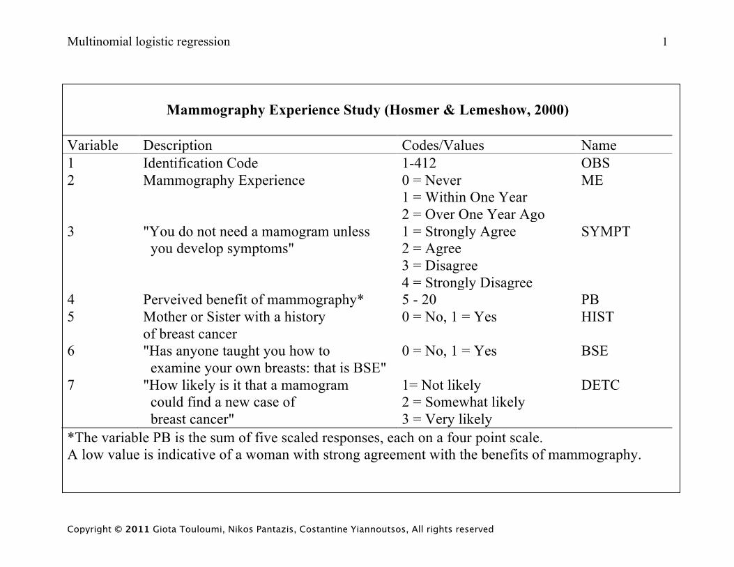
Multinomial logistic regression 1 Copyright © 2011 Giota Touloumi, Nikos Pantazis, Costantine Yiannoutsos, All rights reserved Mammography Experience Study (Hosmer & Lemeshow, 2000) Variable Description Codes/Values Name 1 Identification Code 1-412 OBS 2 Mammography Experience 0 = Never 1 = Within One Year 2 = Over One Year Ago ME 3 "You do not need a mamogram unless you develop symptoms" 1 = Strongly Agree 2 = Agree 3 = Disagree 4 = Strongly Disagree SYMPT 4 Perveived benefit of mammography* 5 - 20 PB 5 Mother or Sister with a history of breast cancer 0 = No, 1 = Yes HIST 6 "Has anyone taught you how to examine your own breasts: that is BSE" 0 = No, 1 = Yes BSE 7 "How likely is it that a mamogram could find a new case of breast cancer" 1= Not likely 2 = Somewhat likely 3 = Very likely DETC *The variable PB is the sum of five scaled responses, each on a four point scale. A low value is indicative of a woman with strong agreement with the benefits of mammography.
Transcript of Multinomial logistic regression 1 - med.uoa.grgtouloum/glm_notes/lecture5.pdf · The multinomial...
Multinomial logistic regression 1
Copyright © 2011 Giota Touloumi, Nikos Pantazis, Costantine Yiannoutsos, All rights reserved
Mammography Experience Study (Hosmer & Lemeshow, 2000)
Variable Description Codes/Values Name 1 Identification Code 1-412 OBS 2 Mammography Experience 0 = Never
1 = Within One Year 2 = Over One Year Ago
ME
3 "You do not need a mamogram unless you develop symptoms"
1 = Strongly Agree 2 = Agree 3 = Disagree 4 = Strongly Disagree
SYMPT
4 Perveived benefit of mammography* 5 - 20 PB 5 Mother or Sister with a history
of breast cancer 0 = No, 1 = Yes HIST
6 "Has anyone taught you how to examine your own breasts: that is BSE"
0 = No, 1 = Yes BSE
7 "How likely is it that a mamogram could find a new case of breast cancer"
1= Not likely 2 = Somewhat likely 3 = Very likely
DETC
*The variable PB is the sum of five scaled responses, each on a four point scale. A low value is indicative of a woman with strong agreement with the benefits of mammography.
Multinomial logistic regression 2
Copyright © 2011 Giota Touloumi, Nikos Pantazis, Costantine Yiannoutsos, All rights reserved
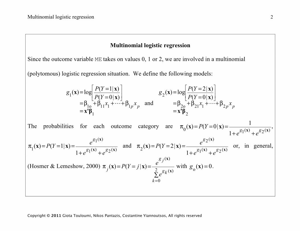
Multinomial logistic regression
Since the outcome variable ME takes on values 0, 1 or 2, we are involved in a multinomial
(polytomous) logistic regression situation. We define the following models:
1
11111o
1 )|0()|1(log)(
βx'
xxx
=β++β+β=
===
⎥⎥⎦
⎤
⎢⎢⎣
⎡
ppxxYPYPg
and
2
2121o2
2 )|0()|2(log)(
βx'
xxx
=β++β+β=
===
⎥⎥⎦
⎤
⎢⎢⎣
⎡
ppxxYPYPg
The probabilities for each outcome category are )(2)(10
1
1)|0()(xx
xxgg ee
YP++
===π ,
)(2)(1
)(1
11
)|1()(xx
xxx
gg
g
ee
eYP++
===π and )(2)(1
)(2
21
)|2()(xx
xxx
gg
g
ee
eYP++
===π or, in general,
(Hosmer & Lemeshow, 2000) ∑
===π
=
2
0
)(
)(
)|()(
k
kg
jg
je
ejYPx
x
xx with 0)(o =xg .
Multinomial logistic regression 3
Copyright © 2011 Giota Touloumi, Nikos Pantazis, Costantine Yiannoutsos, All rights reserved
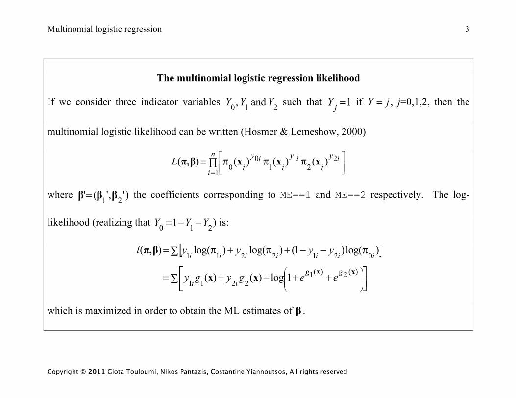
The multinomial logistic regression likelihood
If we consider three indicator variables 210 and , YYY such that 1=jY if jY = , j=0,1,2, then the
multinomial logistic likelihood can be written (Hosmer & Lemeshow, 2000)
∏ ⎥⎦⎤
⎢⎣⎡ πππ=
=
n
i
iyi
iyi
iyiL
1
22
11
00 )()()()( xxxβπ,
where )','(' 21 βββ = the coefficients corresponding to ME==1 and ME==2 respectively. The log-
likelihood (realizing that 210 1 YYY −−= ) is:
[ ]∑ ⎥⎦
⎤⎢⎣⎡ ++−+=
∑ π−−+π+π=
⎟⎟⎠
⎞⎜⎜⎝
⎛ )(2)(12211
0212211
1log)()(
)log()1()log()log()(
xxxx
βπ,
ggii
iiiiiii
eegygy
yyyyl
which is maximized in order to obtain the ML estimates of β .
Multinomial logistic regression 4
Copyright © 2011 Giota Touloumi, Nikos Pantazis, Costantine Yiannoutsos, All rights reserved
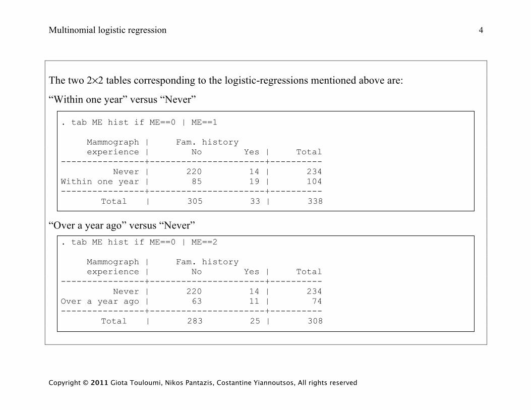
The two 2×2 tables corresponding to the logistic-regressions mentioned above are:
“Within one year” versus “Never”
. tab ME hist if ME==0 | ME==1 Mammograph | Fam. history experience | No Yes | Total ----------------+----------------------+---------- Never | 220 14 | 234 Within one year | 85 19 | 104 ----------------+----------------------+----------
Total | 305 33 | 338
“Over a year ago” versus “Never”
. tab ME hist if ME==0 | ME==2 Mammograph | Fam. history experience | No Yes | Total ----------------+----------------------+---------- Never | 220 14 | 234 Over a year ago | 63 11 | 74 ----------------+----------------------+----------
Total | 283 25 | 308
Multinomial logistic regression 5
Copyright © 2011 Giota Touloumi, Nikos Pantazis, Costantine Yiannoutsos, All rights reserved
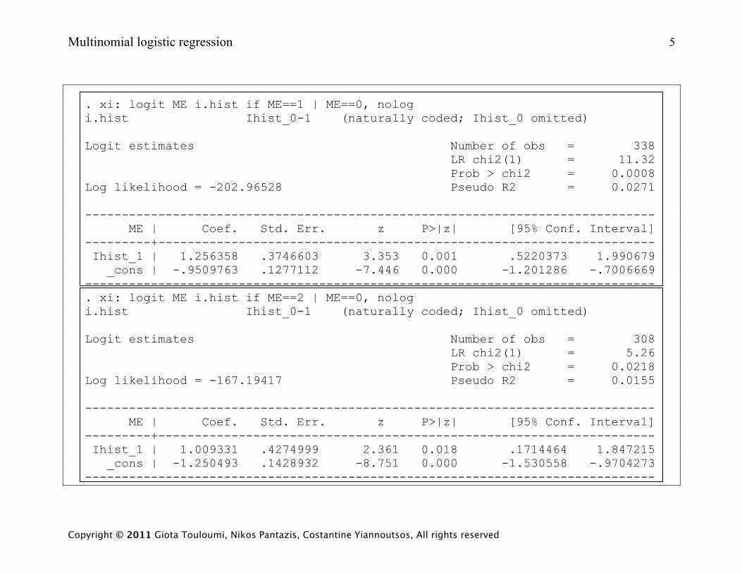
. xi: logit ME i.hist if ME==1 | ME==0, nolog i.hist Ihist_0-1 (naturally coded; Ihist_0 omitted) Logit estimates Number of obs = 338 LR chi2(1) = 11.32 Prob > chi2 = 0.0008 Log likelihood = -202.96528 Pseudo R2 = 0.0271 ------------------------------------------------------------------------------ ME | Coef. Std. Err. z P>|z| [95% Conf. Interval] ---------+-------------------------------------------------------------------- Ihist_1 | 1.256358 .3746603 3.353 0.001 .5220373 1.990679 _cons | -.9509763 .1277112 -7.446 0.000 -1.201286 -.7006669 ------------------------------------------------------------------------------ . xi: logit ME i.hist if ME==2 | ME==0, nolog i.hist Ihist_0-1 (naturally coded; Ihist_0 omitted) Logit estimates Number of obs = 308 LR chi2(1) = 5.26 Prob > chi2 = 0.0218 Log likelihood = -167.19417 Pseudo R2 = 0.0155 ------------------------------------------------------------------------------ ME | Coef. Std. Err. z P>|z| [95% Conf. Interval] ---------+-------------------------------------------------------------------- Ihist_1 | 1.009331 .4274999 2.361 0.018 .1714464 1.847215 _cons | -1.250493 .1428932 -8.751 0.000 -1.530558 -.9704273 ------------------------------------------------------------------------------
Multinomial logistic regression 6
Copyright © 2011 Giota Touloumi, Nikos Pantazis, Costantine Yiannoutsos, All rights reserved
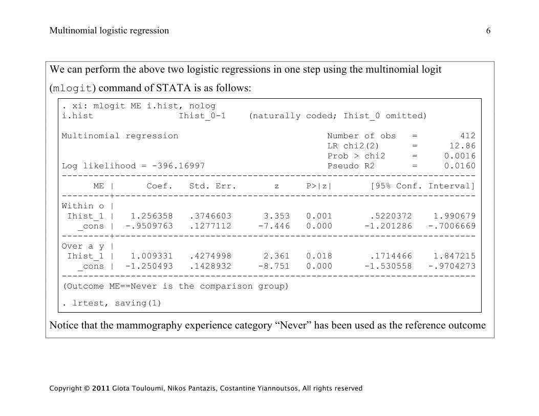
We can perform the above two logistic regressions in one step using the multinomial logit
(mlogit) command of STATA is as follows: . xi: mlogit ME i.hist, nolog i.hist Ihist_0-1 (naturally coded; Ihist_0 omitted) Multinomial regression Number of obs = 412 LR chi2(2) = 12.86 Prob > chi2 = 0.0016 Log likelihood = -396.16997 Pseudo R2 = 0.0160 ------------------------------------------------------------------------------ ME | Coef. Std. Err. z P>|z| [95% Conf. Interval] ---------+-------------------------------------------------------------------- Within o | Ihist_1 | 1.256358 .3746603 3.353 0.001 .5220372 1.990679 _cons | -.9509763 .1277112 -7.446 0.000 -1.201286 -.7006669 ---------+-------------------------------------------------------------------- Over a y | Ihist_1 | 1.009331 .4274998 2.361 0.018 .1714466 1.847215 _cons | -1.250493 .1428932 -8.751 0.000 -1.530558 -.9704273 ------------------------------------------------------------------------------ (Outcome ME==Never is the comparison group)
. lrtest, saving(1)
Notice that the mammography experience category “Never” has been used as the reference outcome
Multinomial logistic regression 7
Copyright © 2011 Giota Touloumi, Nikos Pantazis, Costantine Yiannoutsos, All rights reserved
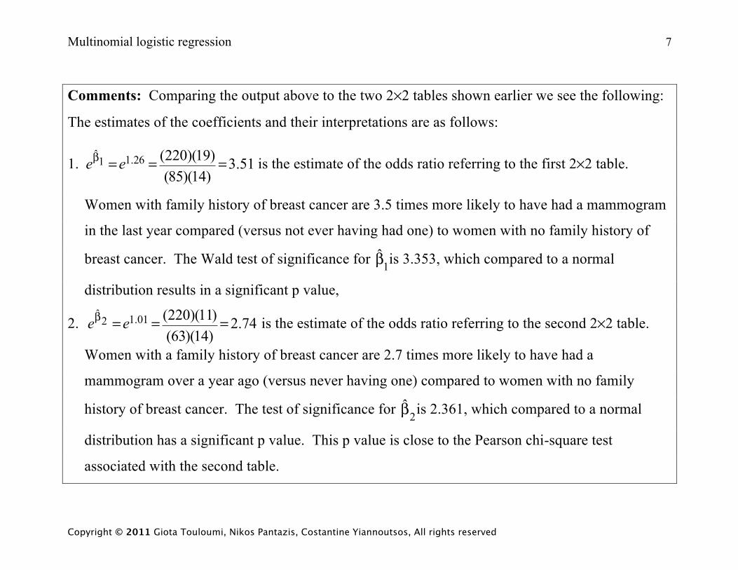
Comments: Comparing the output above to the two 2×2 tables shown earlier we see the following:
The estimates of the coefficients and their interpretations are as follows:
1. 51.3)14)(85()19)(220(26.11
ˆ===β ee is the estimate of the odds ratio referring to the first 2×2 table.
Women with family history of breast cancer are 3.5 times more likely to have had a mammogram
in the last year compared (versus not ever having had one) to women with no family history of
breast cancer. The Wald test of significance for 1β̂ is 3.353, which compared to a normal
distribution results in a significant p value,
2. 74.2)14)(63()11)(220(01.12
ˆ===β ee is the estimate of the odds ratio referring to the second 2×2 table.
Women with a family history of breast cancer are 2.7 times more likely to have had a
mammogram over a year ago (versus never having one) compared to women with no family
history of breast cancer. The test of significance for 2β̂ is 2.361, which compared to a normal
distribution has a significant p value. This p value is close to the Pearson chi-square test
associated with the second table.
Multinomial logistic regression 8
Copyright © 2011 Giota Touloumi, Nikos Pantazis, Costantine Yiannoutsos, All rights reserved
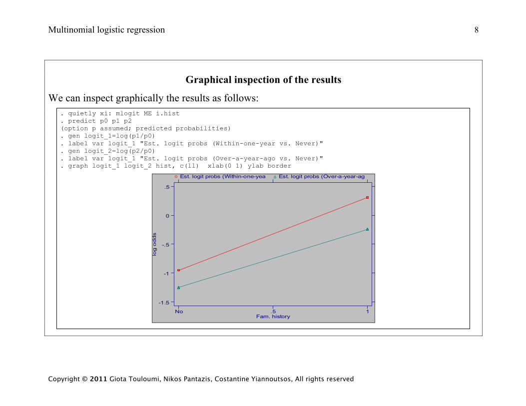
Graphical inspection of the results
We can inspect graphically the results as follows: . quietly xi: mlogit ME i.hist . predict p0 p1 p2 (option p assumed; predicted probabilities) . gen logit_1=log(p1/p0) . label var logit_1 "Est. logit probs (Within-one-year vs. Never)" . gen logit_2=log(p2/p0) . label var logit_1 "Est. logit probs (Over-a-year-ago vs. Never)" . graph logit_1 logit_2 hist, c(ll) xlab(0 1) ylab border
log o
dds
Fam. history
Est. logit probs (Within-one-yea Est. logit probs (Over-a-year-ag
No .5 1
-1.5
-1
-.5
0
.5
Multinomial logistic regression 9
Copyright © 2011 Giota Touloumi, Nikos Pantazis, Costantine Yiannoutsos, All rights reserved
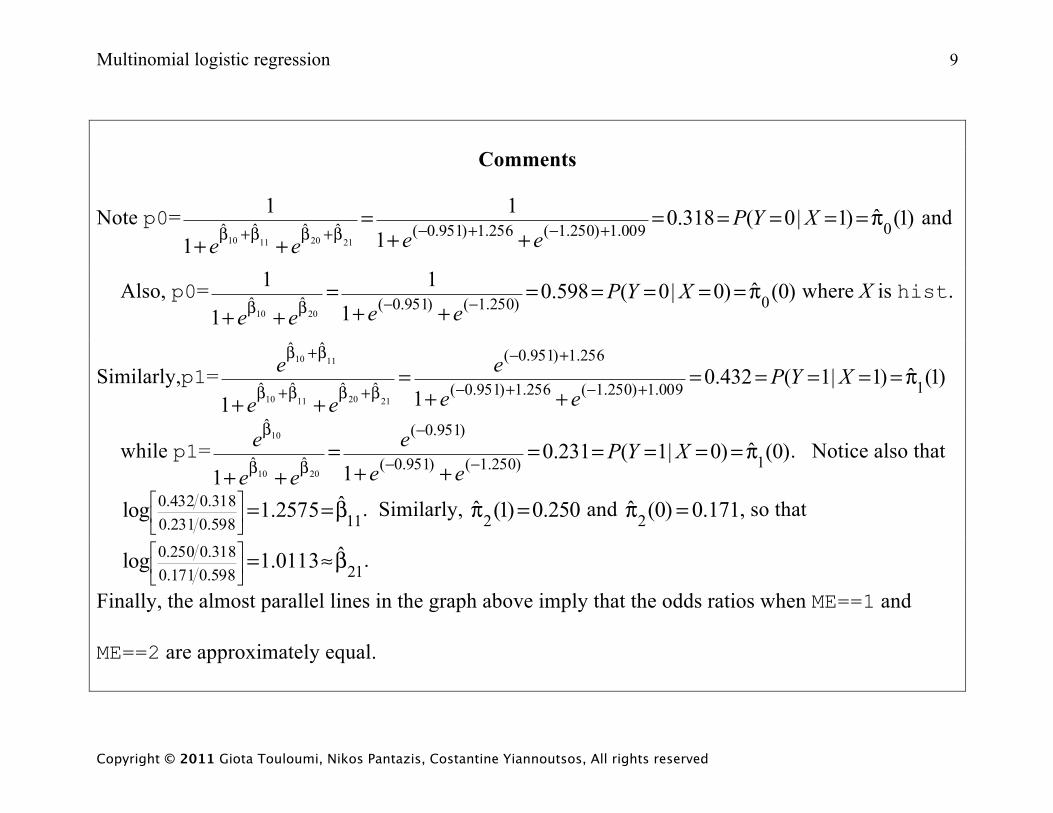
Comments
Note p0= )1(ˆ)1|0(318.01
1
1
10009.1)250.1(256.1)951.0(ˆˆˆˆ
21201110
π=====++
=++
+−+−β+ββ+βXYP
eeee and
Also, p0= )0(ˆ)0|0(598.01
1
1
10)250.1()951.0(ˆˆ
2010
π=====++
=++
−−ββXYP
eeee where X is hist.
Similarly,p1= )1(ˆ)1|1(432.011
1009.1)250.1(256.1)951.0(
256.1)951.0(
ˆˆˆˆ
ˆˆ
21201110
1110
π=====++
=++
+−+−
+−
β+ββ+β
β+βXYP
eee
ee
e
while p1= )0(ˆ)0|1(231.011
1)250.1()951.0(
)951.0(
ˆˆ
ˆ
2010
10
π=====++
=++
−−
−
ββ
βXYP
eee
ee
e . Notice also that
11598.0231.0318.0432.0 ˆ2575.1log β==⎥
⎦
⎤⎢⎣
⎡ . Similarly, 250.0)1(ˆ 2 =π and 171.0)0(ˆ 2 =π , so that
21598.0171.0318.0250.0 ˆ0113.1log β≈=⎥
⎦
⎤⎢⎣
⎡ .
Finally, the almost parallel lines in the graph above imply that the odds ratios when ME==1 and
ME==2 are approximately equal.
Multinomial logistic regression 10
Copyright © 2011 Giota Touloumi, Nikos Pantazis, Costantine Yiannoutsos, All rights reserved
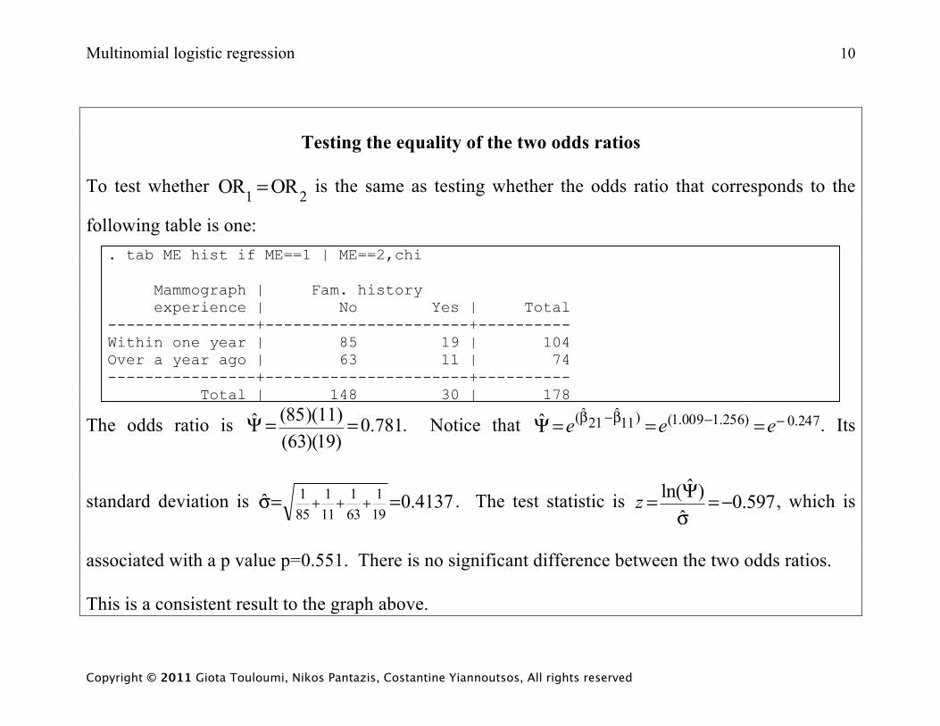
Testing the equality of the two odds ratios
To test whether 21 OROR = is the same as testing whether the odds ratio that corresponds to the
following table is one: . tab ME hist if ME==1 | ME==2,chi Mammograph | Fam. history experience | No Yes | Total ----------------+----------------------+---------- Within one year | 85 19 | 104 Over a year ago | 63 11 | 74 ----------------+----------------------+---------- Total | 148 30 | 178
The odds ratio is 781.0)19)(63(
(85)(11)ˆ ==Ψ . Notice that 247.0)256.1009.1()11ˆ
21ˆ(ˆ −−β−β ===Ψ eee . Its
standard deviation is 4137.0ˆ191
631
111
851 ==σ +++ . The test statistic is 597.0
ˆ)ˆln( −=
σΨ=z , which is
associated with a p value p=0.551. There is no significant difference between the two odds ratios.
This is a consistent result to the graph above.
Multinomial logistic regression 11
Copyright © 2011 Giota Touloumi, Nikos Pantazis, Costantine Yiannoutsos, All rights reserved
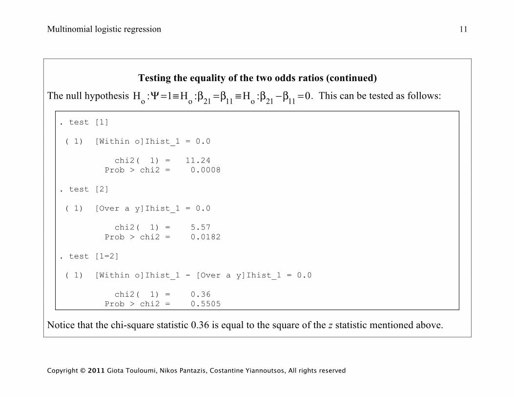
Testing the equality of the two odds ratios (continued)
The null hypothesis 0:H:H1:H 1121o1121oo =β−β≡β=β≡=Ψ . This can be tested as follows:
. test [1] ( 1) [Within o]Ihist_1 = 0.0 chi2( 1) = 11.24 Prob > chi2 = 0.0008 . test [2] ( 1) [Over a y]Ihist_1 = 0.0 chi2( 1) = 5.57 Prob > chi2 = 0.0182 . test [1=2] ( 1) [Within o]Ihist_1 - [Over a y]Ihist_1 = 0.0 chi2( 1) = 0.36 Prob > chi2 = 0.5505
Notice that the chi-square statistic 0.36 is equal to the square of the z statistic mentioned above.
Multinomial logistic regression 12
Copyright © 2011 Giota Touloumi, Nikos Pantazis, Costantine Yiannoutsos, All rights reserved
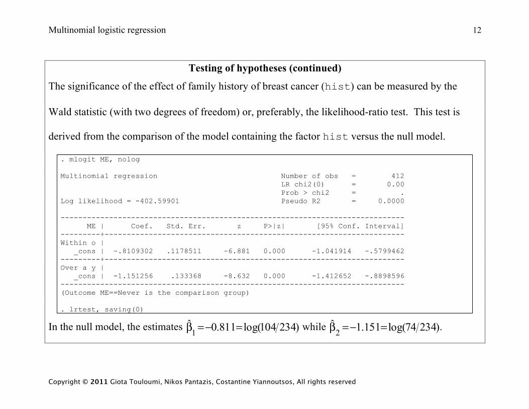
Testing of hypotheses (continued)
The significance of the effect of family history of breast cancer (hist) can be measured by the
Wald statistic (with two degrees of freedom) or, preferably, the likelihood-ratio test. This test is
derived from the comparison of the model containing the factor hist versus the null model.
. mlogit ME, nolog Multinomial regression Number of obs = 412 LR chi2(0) = 0.00 Prob > chi2 = . Log likelihood = -402.59901 Pseudo R2 = 0.0000 ------------------------------------------------------------------------------ ME | Coef. Std. Err. z P>|z| [95% Conf. Interval] ---------+-------------------------------------------------------------------- Within o | _cons | -.8109302 .1178511 -6.881 0.000 -1.041914 -.5799462 ---------+-------------------------------------------------------------------- Over a y | _cons | -1.151256 .133368 -8.632 0.000 -1.412652 -.8898596 ------------------------------------------------------------------------------ (Outcome ME==Never is the comparison group) . lrtest, saving(0)
In the null model, the estimates )234104log(811.0ˆ1 =−=β while )23474log(151.1ˆ
2 =−=β .
Multinomial logistic regression 13
Copyright © 2011 Giota Touloumi, Nikos Pantazis, Costantine Yiannoutsos, All rights reserved
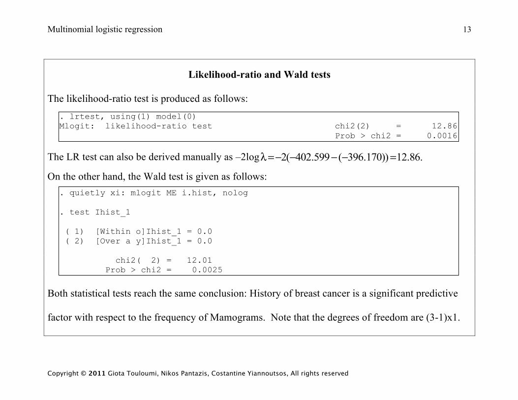
Likelihood-ratio and Wald tests
The likelihood-ratio test is produced as follows:
. lrtest, using(1) model(0) Mlogit: likelihood-ratio test chi2(2) = 12.86 Prob > chi2 = 0.0016
The LR test can also be derived manually as –2log .86.12))170.396(599.402(2 =−−−−=λ
On the other hand, the Wald test is given as follows: . quietly xi: mlogit ME i.hist, nolog . test Ihist_1 ( 1) [Within o]Ihist_1 = 0.0 ( 2) [Over a y]Ihist_1 = 0.0 chi2( 2) = 12.01 Prob > chi2 = 0.0025
Both statistical tests reach the same conclusion: History of breast cancer is a significant predictive
factor with respect to the frequency of Mamograms. Note that the degrees of freedom are (3-1)x1.
Multinomial logistic regression 14
Copyright © 2011 Giota Touloumi, Nikos Pantazis, Costantine Yiannoutsos, All rights reserved
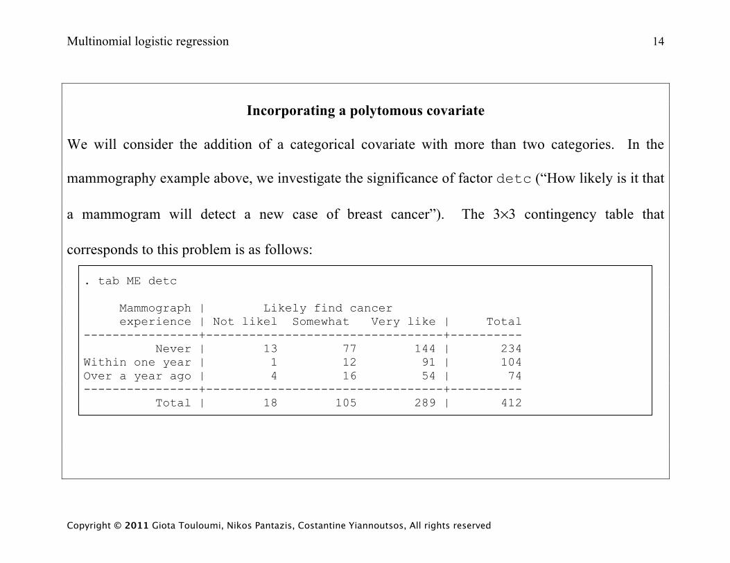
Incorporating a polytomous covariate
We will consider the addition of a categorical covariate with more than two categories. In the
mammography example above, we investigate the significance of factor detc (“How likely is it that
a mammogram will detect a new case of breast cancer”). The 3×3 contingency table that
corresponds to this problem is as follows:
. tab ME detc Mammograph | Likely find cancer experience | Not likel Somewhat Very like | Total ----------------+---------------------------------+---------- Never | 13 77 144 | 234 Within one year | 1 12 91 | 104 Over a year ago | 4 16 54 | 74 ----------------+---------------------------------+---------- Total | 18 105 289 | 412
Multinomial logistic regression 15
Copyright © 2011 Giota Touloumi, Nikos Pantazis, Costantine Yiannoutsos, All rights reserved
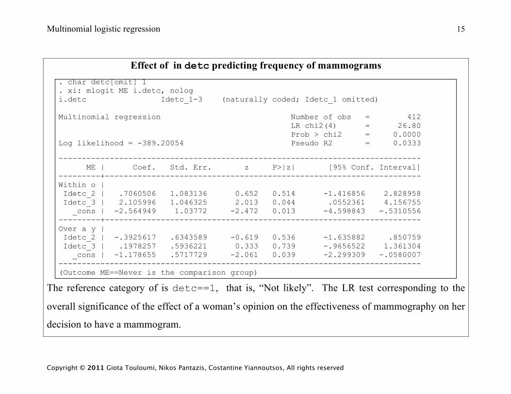
Effect of in detc predicting frequency of mammograms . char detc[omit] 1 . xi: mlogit ME i.detc, nolog i.detc Idetc_1-3 (naturally coded; Idetc_1 omitted) Multinomial regression Number of obs = 412 LR chi2(4) = 26.80 Prob > chi2 = 0.0000 Log likelihood = -389.20054 Pseudo R2 = 0.0333 ------------------------------------------------------------------------------ ME | Coef. Std. Err. z P>|z| [95% Conf. Interval] ---------+-------------------------------------------------------------------- Within o | Idetc_2 | .7060506 1.083136 0.652 0.514 -1.416856 2.828958 Idetc_3 | 2.105996 1.046325 2.013 0.044 .0552361 4.156755 _cons | -2.564949 1.03772 -2.472 0.013 -4.598843 -.5310556 ---------+-------------------------------------------------------------------- Over a y | Idetc_2 | -.3925617 .6343589 -0.619 0.536 -1.635882 .850759 Idetc_3 | .1978257 .5936221 0.333 0.739 -.9656522 1.361304 _cons | -1.178655 .5717729 -2.061 0.039 -2.299309 -.0580007 ------------------------------------------------------------------------------ (Outcome ME==Never is the comparison group)
The reference category of is detc==1, that is, “Not likely”. The LR test corresponding to the
overall significance of the effect of a woman’s opinion on the effectiveness of mammography on her
decision to have a mammogram.
Multinomial logistic regression 16
Copyright © 2011 Giota Touloumi, Nikos Pantazis, Costantine Yiannoutsos, All rights reserved
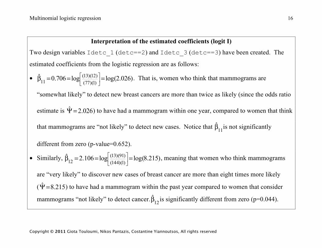
Interpretation of the estimated coefficients (logit I)
Two design variables Idetc_1 (detc==2) and Idetc_3 (detc==3) have been created. The
estimated coefficients from the logistic regression are as follows:
• )026.2log(log706.0ˆ)1)(77()12)(13(
11 ===β ⎥⎦
⎤⎢⎣
⎡ . That is, women who think that mammograms are
“somewhat likely” to detect new breast cancers are more than twice as likely (since the odds ratio
estimate is 026.2ˆ =Ψ ) to have had a mammogram within one year, compared to women that think
that mammograms are “not likely” to detect new cases. Notice that 11β̂ is not significantly
different from zero (p-value=0.652).
• Similarly, )215.8log(log106.2ˆ)1)(144()91)(13(
12 ===β ⎥⎦
⎤⎢⎣
⎡ , meaning that women who think mammograms
are “very likely” to discover new cases of breast cancer are more than eight times more likely
( 215.8ˆ =Ψ ) to have had a mammogram within the past year compared to women that consider
mammograms “not likely” to detect cancer. 12β̂ is significantly different from zero (p=0.044).
Multinomial logistic regression 17
Copyright © 2011 Giota Touloumi, Nikos Pantazis, Costantine Yiannoutsos, All rights reserved
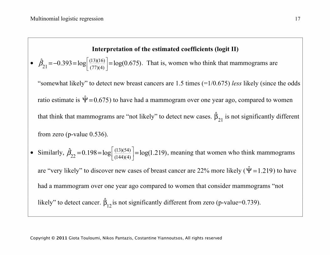
Interpretation of the estimated coefficients (logit II)
• (13)(16)21 (77)(4)ˆ 0.393 log log(0.675)β ⎡ ⎤
⎢ ⎥⎣ ⎦
=− = = . That is, women who think that mammograms are
“somewhat likely” to detect new breast cancers are 1.5 times (=1/0.675) less likely (since the odds
ratio estimate is 675.0ˆ =Ψ ) to have had a mammogram over one year ago, compared to women
that think that mammograms are “not likely” to detect new cases. 21β̂ is not significantly different
from zero (p-value 0.536).
• Similarly, (13)(54)22 (144)(4)ˆ 0.198 log log(1.219)β ⎡ ⎤
⎢ ⎥⎣ ⎦
= = = , meaning that women who think mammograms
are “very likely” to discover new cases of breast cancer are 22% more likely ( 219.1ˆ =Ψ ) to have
had a mammogram over one year ago compared to women that consider mammograms “not
likely” to detect cancer. 12β̂ is not significantly different from zero (p-value=0.739).
Multinomial logistic regression 18
Copyright © 2011 Giota Touloumi, Nikos Pantazis, Costantine Yiannoutsos, All rights reserved
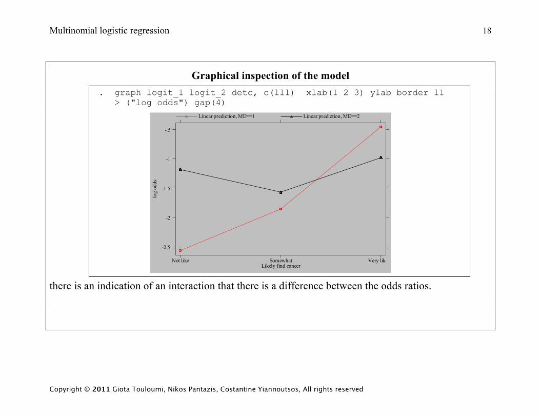
Graphical inspection of the model . graph logit_1 logit_2 detc, c(lll) xlab(1 2 3) ylab border l1 > ("log odds") gap(4)
log
odds
Likely find cancer
Linear prediction, ME==1 Linear prediction, ME==2
Not like Somewhat Very lik
-2.5
-2
-1.5
-1
-.5
there is an indication of an interaction that there is a difference between the odds ratios.
Multinomial logistic regression 19
Copyright © 2011 Giota Touloumi, Nikos Pantazis, Costantine Yiannoutsos, All rights reserved
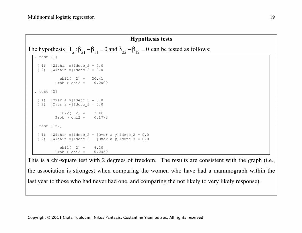
Hypothesis tests
The hypothesis 0 and 0:H 12221121o =β−β=β−β can be tested as follows: . test [1] ( 1) [Within o]Idetc_2 = 0.0 ( 2) [Within o]Idetc_3 = 0.0 chi2( 2) = 20.41 Prob > chi2 = 0.0000 . test [2] ( 1) [Over a y]Idetc_2 = 0.0 ( 2) [Over a y]Idetc_3 = 0.0 chi2( 2) = 3.46 Prob > chi2 = 0.1773 . test [1=2] ( 1) [Within o]Idetc_2 - [Over a y]Idetc_2 = 0.0 ( 2) [Within o]Idetc_3 - [Over a y]Idetc_3 = 0.0 chi2( 2) = 6.20 Prob > chi2 = 0.0450
This is a chi-square test with 2 degrees of freedom. The results are consistent with the graph (i.e.,
the association is strongest when comparing the women who have had a mammograph within the
last year to those who had never had one, and comparing the not likely to very likely response).
Multinomial logistic regression 20
Copyright © 2011 Giota Touloumi, Nikos Pantazis, Costantine Yiannoutsos, All rights reserved
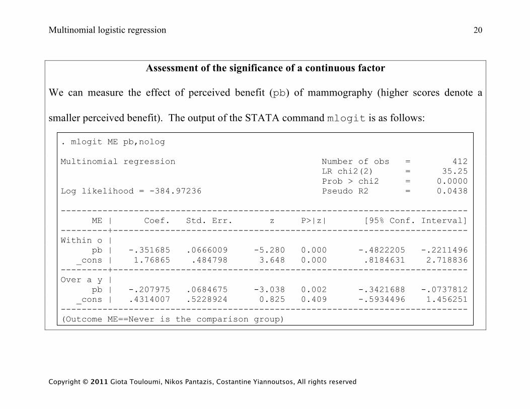
Assessment of the significance of a continuous factor
We can measure the effect of perceived benefit (pb) of mammography (higher scores denote a
smaller perceived benefit). The output of the STATA command mlogit is as follows:
. mlogit ME pb,nolog Multinomial regression Number of obs = 412 LR chi2(2) = 35.25 Prob > chi2 = 0.0000 Log likelihood = -384.97236 Pseudo R2 = 0.0438 ------------------------------------------------------------------------------ ME | Coef. Std. Err. z P>|z| [95% Conf. Interval] ---------+-------------------------------------------------------------------- Within o | pb | -.351685 .0666009 -5.280 0.000 -.4822205 -.2211496 _cons | 1.76865 .484798 3.648 0.000 .8184631 2.718836 ---------+-------------------------------------------------------------------- Over a y | pb | -.207975 .0684675 -3.038 0.002 -.3421688 -.0737812 _cons | .4314007 .5228924 0.825 0.409 -.5934496 1.456251 ------------------------------------------------------------------------------ (Outcome ME==Never is the comparison group)
Multinomial logistic regression 21
Copyright © 2011 Giota Touloumi, Nikos Pantazis, Costantine Yiannoutsos, All rights reserved
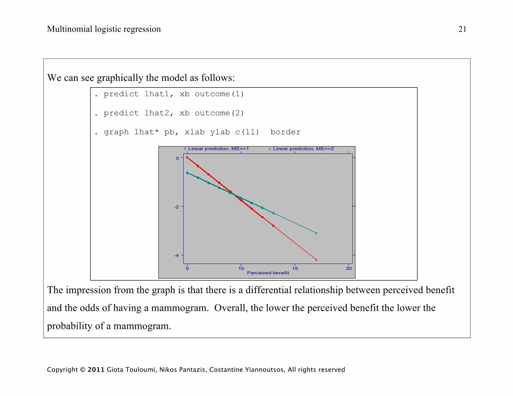
We can see graphically the model as follows:
. predict lhat1, xb outcome(1) . predict lhat2, xb outcome(2) . graph lhat* pb, xlab ylab c(ll) border
Perceived benefit
Linear prediction, ME==1 Linear prediction, ME==2
5 10 15 20
-4
-2
0
The impression from the graph is that there is a differential relationship between perceived benefit
and the odds of having a mammogram. Overall, the lower the perceived benefit the lower the
probability of a mammogram.
Multinomial logistic regression 22
Copyright © 2011 Giota Touloumi, Nikos Pantazis, Costantine Yiannoutsos, All rights reserved
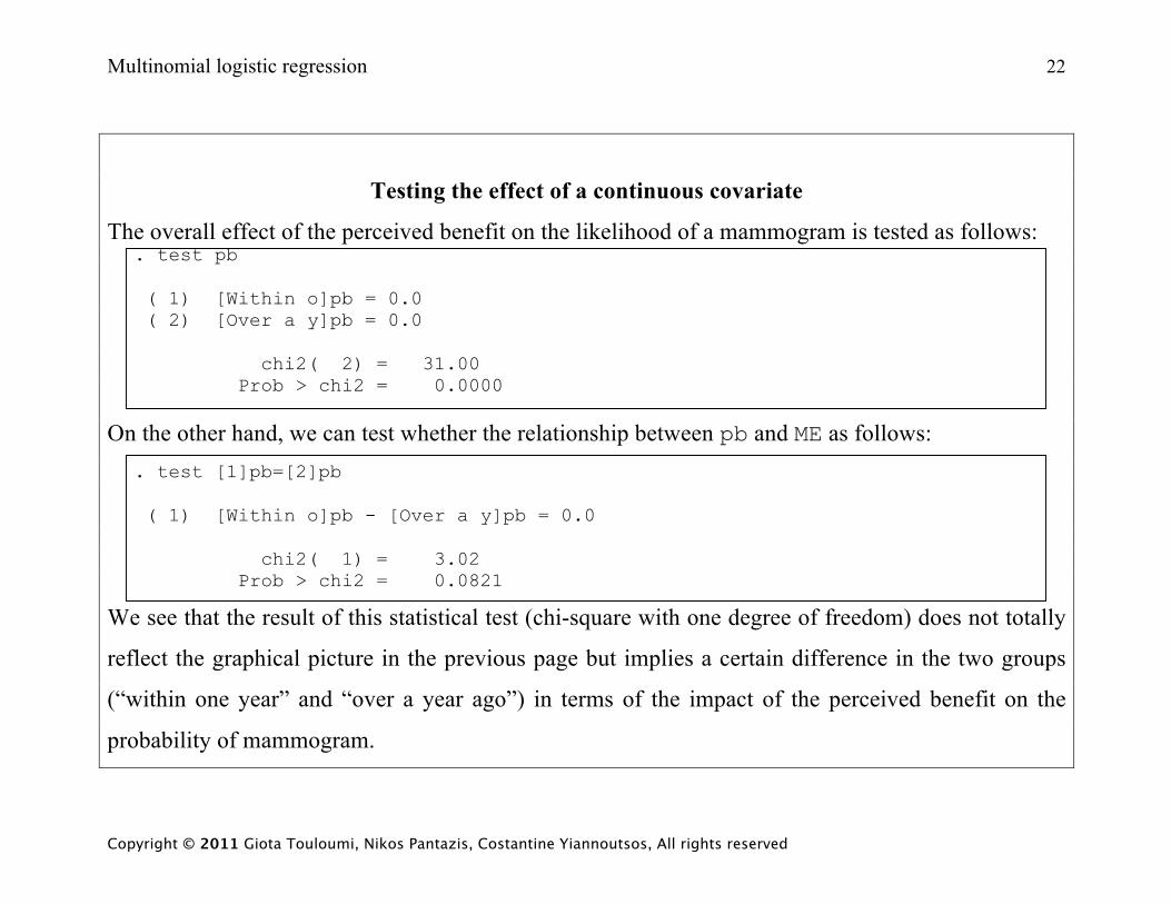
Testing the effect of a continuous covariate
The overall effect of the perceived benefit on the likelihood of a mammogram is tested as follows: . test pb ( 1) [Within o]pb = 0.0 ( 2) [Over a y]pb = 0.0 chi2( 2) = 31.00 Prob > chi2 = 0.0000
On the other hand, we can test whether the relationship between pb and ME as follows: . test [1]pb=[2]pb ( 1) [Within o]pb - [Over a y]pb = 0.0 chi2( 1) = 3.02 Prob > chi2 = 0.0821
We see that the result of this statistical test (chi-square with one degree of freedom) does not totally
reflect the graphical picture in the previous page but implies a certain difference in the two groups
(“within one year” and “over a year ago”) in terms of the impact of the perceived benefit on the
probability of mammogram.
Multinomial logistic regression 23
Copyright © 2011 Giota Touloumi, Nikos Pantazis, Costantine Yiannoutsos, All rights reserved
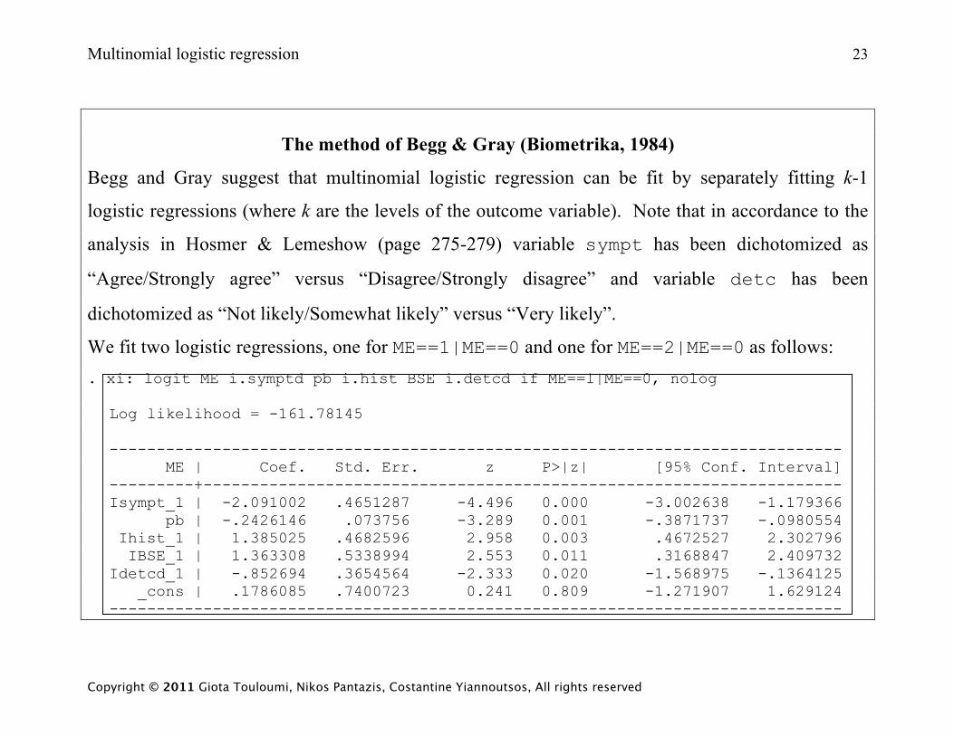
The method of Begg & Gray (Biometrika, 1984)
Begg and Gray suggest that multinomial logistic regression can be fit by separately fitting k-1
logistic regressions (where k are the levels of the outcome variable). Note that in accordance to the
analysis in Hosmer & Lemeshow (page 275-279) variable sympt has been dichotomized as
“Agree/Strongly agree” versus “Disagree/Strongly disagree” and variable detc has been
dichotomized as “Not likely/Somewhat likely” versus “Very likely”.
We fit two logistic regressions, one for ME==1|ME==0 and one for ME==2|ME==0 as follows: . xi: logit ME i.symptd pb i.hist BSE i.detcd if ME==1|ME==0, nolog
Log likelihood = -161.78145 ------------------------------------------------------------------------------ ME | Coef. Std. Err. z P>|z| [95% Conf. Interval] ---------+-------------------------------------------------------------------- Isympt_1 | -2.091002 .4651287 -4.496 0.000 -3.002638 -1.179366 pb | -.2426146 .073756 -3.289 0.001 -.3871737 -.0980554 Ihist_1 | 1.385025 .4682596 2.958 0.003 .4672527 2.302796 IBSE_1 | 1.363308 .5338994 2.553 0.011 .3168847 2.409732 Idetcd_1 | -.852694 .3654564 -2.333 0.020 -1.568975 -.1364125 _cons | .1786085 .7400723 0.241 0.809 -1.271907 1.629124 ------------------------------------------------------------------------------
Multinomial logistic regression 24
Copyright © 2011 Giota Touloumi, Nikos Pantazis, Costantine Yiannoutsos, All rights reserved
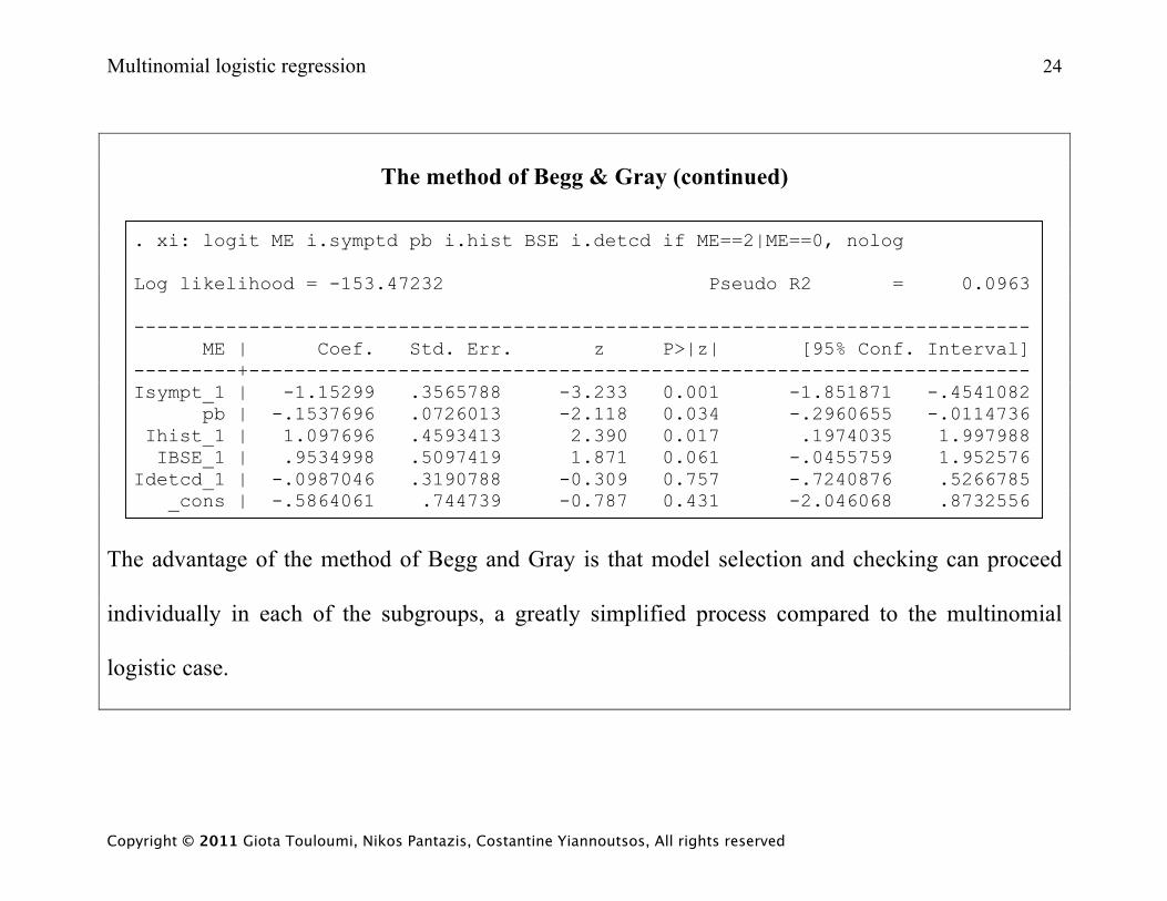
The method of Begg & Gray (continued)
. xi: logit ME i.symptd pb i.hist BSE i.detcd if ME==2|ME==0, nolog Log likelihood = -153.47232 Pseudo R2 = 0.0963 ------------------------------------------------------------------------------ ME | Coef. Std. Err. z P>|z| [95% Conf. Interval] ---------+-------------------------------------------------------------------- Isympt_1 | -1.15299 .3565788 -3.233 0.001 -1.851871 -.4541082 pb | -.1537696 .0726013 -2.118 0.034 -.2960655 -.0114736 Ihist_1 | 1.097696 .4593413 2.390 0.017 .1974035 1.997988 IBSE_1 | .9534998 .5097419 1.871 0.061 -.0455759 1.952576 Idetcd_1 | -.0987046 .3190788 -0.309 0.757 -.7240876 .5266785 _cons | -.5864061 .744739 -0.787 0.431 -2.046068 .8732556
The advantage of the method of Begg and Gray is that model selection and checking can proceed
individually in each of the subgroups, a greatly simplified process compared to the multinomial
logistic case.
Multinomial logistic regression 25
Copyright © 2011 Giota Touloumi, Nikos Pantazis, Costantine Yiannoutsos, All rights reserved
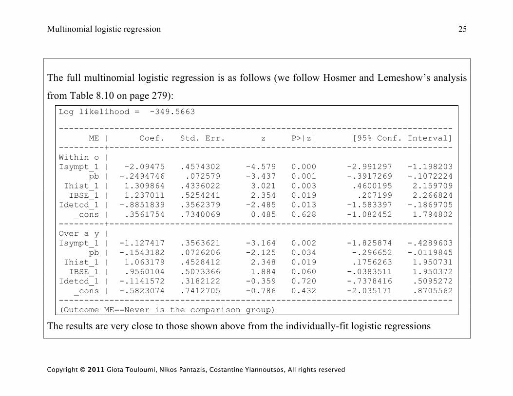
The full multinomial logistic regression is as follows (we follow Hosmer and Lemeshow’s analysis
from Table 8.10 on page 279): Log likelihood = -349.5663 ------------------------------------------------------------------------------ ME | Coef. Std. Err. z P>|z| [95% Conf. Interval] ---------+-------------------------------------------------------------------- Within o | Isympt_1 | -2.09475 .4574302 -4.579 0.000 -2.991297 -1.198203 pb | -.2494746 .072579 -3.437 0.001 -.3917269 -.1072224 Ihist_1 | 1.309864 .4336022 3.021 0.003 .4600195 2.159709 IBSE_1 | 1.237011 .5254241 2.354 0.019 .207199 2.266824 Idetcd_1 | -.8851839 .3562379 -2.485 0.013 -1.583397 -.1869705 _cons | .3561754 .7340069 0.485 0.628 -1.082452 1.794802 ---------+-------------------------------------------------------------------- Over a y | Isympt_1 | -1.127417 .3563621 -3.164 0.002 -1.825874 -.4289603 pb | -.1543182 .0726206 -2.125 0.034 -.296652 -.0119845 Ihist_1 | 1.063179 .4528412 2.348 0.019 .1756263 1.950731 IBSE_1 | .9560104 .5073366 1.884 0.060 -.0383511 1.950372 Idetcd_1 | -.1141572 .3182122 -0.359 0.720 -.7378416 .5095272 _cons | -.5823074 .7412705 -0.786 0.432 -2.035171 .8705562 ------------------------------------------------------------------------------ (Outcome ME==Never is the comparison group)
The results are very close to those shown above from the individually-fit logistic regressions
Multinomial logistic regression 26
Copyright © 2011 Giota Touloumi, Nikos Pantazis, Costantine Yiannoutsos, All rights reserved
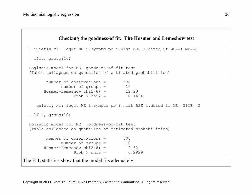
Checking the goodness-of fit: The Hosmer and Lemeshow test
. quietly xi: logit ME i.symptd pb i.hist BSE i.detcd if ME==1|ME==0
. lfit, group(10) Logistic model for ME, goodness-of-fit test (Table collapsed on quantiles of estimated probabilities) number of observations = 338 number of groups = 10 Hosmer-Lemeshow chi2(8) = 12.20 Prob > chi2 = 0.1424 . quietly xi: logit ME i.symptd pb i.hist BSE i.detcd if ME==2|ME==0 . lfit, group(10) Logistic model for ME, goodness-of-fit test (Table collapsed on quantiles of estimated probabilities) number of observations = 308 number of groups = 10 Hosmer-Lemeshow chi2(8) = 9.62 Prob > chi2 = 0.2929
The H-L statistics show that the model fits adequately.
Multinomial logistic regression 27
Copyright © 2011 Giota Touloumi, Nikos Pantazis, Costantine Yiannoutsos, All rights reserved
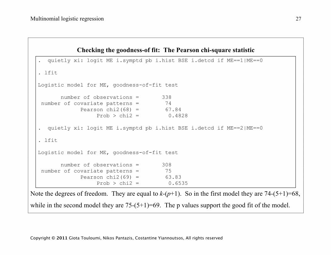
Checking the goodness-of fit: The Pearson chi-square statistic
. quietly xi: logit ME i.symptd pb i.hist BSE i.detcd if ME==1|ME==0 . lfit Logistic model for ME, goodness-of-fit test number of observations = 338 number of covariate patterns = 74 Pearson chi2(68) = 67.84 Prob > chi2 = 0.4828 . quietly xi: logit ME i.symptd pb i.hist BSE i.detcd if ME==2|ME==0 . lfit Logistic model for ME, goodness-of-fit test number of observations = 308 number of covariate patterns = 75 Pearson chi2(69) = 63.83 Prob > chi2 = 0.6535
Note the degrees of freedom. They are equal to k-(p+1). So in the first model they are 74-(5+1)=68,
while in the second model they are 75-(5+1)=69. The p values support the good fit of the model.

Multinomial logistic regression 28
Copyright © 2011 Giota Touloumi, Nikos Pantazis, Costantine Yiannoutsos, All rights reserved
Checking the goodness-of fit: The Stukel test* (JASA, 1988)
The Stukel test is implemented as follows (Hosmer & Lemeshow, page 155):
Step 1: Produce the predicted probabilities jπ̂ , j=1,…,k over all covariate patterns k.
Step 2. Produce the fitted logits kjg 'jj
j
j ,...,1 ,ˆlogˆˆ1
ˆ=== ⎟
⎟
⎠
⎞⎜⎜
⎝
⎛
π−
πβx over all covariate patterns k.
Step 3. Compute two new covariates )5.0ˆ(Iˆ5.0 21 ≥π××−= jjj gz and 2
2 ˆ ˆ(0.5) I( 0.5)j j jz g π= × × <
Step 4. Perform the Score test for the addition of z1 and z2 into the model. Alternatively, we can
perform the likelihood-ratio test.
__________________ * Optional topic
Multinomial logistic regression 29
Copyright © 2011 Giota Touloumi, Nikos Pantazis, Costantine Yiannoutsos, All rights reserved
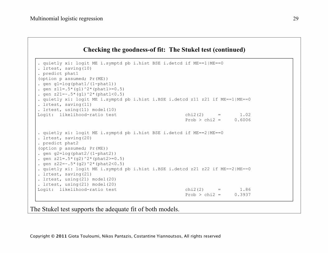
Checking the goodness-of fit: The Stukel test (continued)
. quietly xi: logit ME i.symptd pb i.hist BSE i.detcd if ME==1|ME==0
. lrtest, saving(10)
. predict phat1 (option p assumed; Pr(ME)) . gen g1=log(phat1/(1-phat1)) . gen z11=.5*(g1)^2*(phat1>=0.5) . gen z21=-.5*(g1)^2*(phat1<0.5) . quietly xi: logit ME i.symptd pb i.hist i.BSE i.detcd z11 z21 if ME==1|ME==0 . lrtest, saving(11) . lrtest, using(11) model(10) Logit: likelihood-ratio test chi2(2) = 1.02 Prob > chi2 = 0.6006
. quietly xi: logit ME i.symptd pb i.hist BSE i.detcd if ME==2|ME==0 . lrtest, saving(20) . predict phat2 (option p assumed; Pr(ME)) . gen g2=log(phat2/(1-phat2)) . gen z21=.5*(g2)^2*(phat2>=0.5) . gen z22=-.5*(g2)^2*(phat2<0.5) . quietly xi: logit ME i.symptd pb i.hist i.BSE i.detcd z21 z22 if ME==2|ME==0 . lrtest, saving(21) . lrtest, using(21) model(20) . lrtest, using(21) model(20) Logit: likelihood-ratio test chi2(2) = 1.86 Prob > chi2 = 0.3937
The Stukel test supports the adequate fit of both models.