Multinomial Choice Models -...

Multinomial Choice Models

January 17, 2012

() Applied Economoetrics: Topic 3 January 17, 2012 1 / 40

Introduction

Last lecture slides covered case where dependent variable re�ectedchoice between 2 options

Multinomial choice models are used when more than two options

Much of the theory and intuition is similar to bivariate choice, butsome new issues arise

Most commonly used models are extensions of probit and logit

Multinomial probit, multinomial logit and conditional logit

Reading: Koop (2008, pages 287-296) and Gujarati (chapter 9)


Empirical Example 1

Example taken from marketing literature

Data from N = 136 households in Rome, Georgia.

Data taken from supermarket optical scanners.

Which of four brands of crackers (Sunshine, Keebler, Nabisco andPrivate label) did each household purchase

As explanatory variable: the price of all four brands of crackers in thestore at time of purchase as explanatory variables.


For future reference, note the following properties of this example:

Note 1: The explanatory variable is a characteristic of the crackersNOT the households

Attribute of the choice NOT an attribute of the individual

Note 2: The options the household faces are unordered

In contrast, some applications involve an ordered choice set

E.g. Consumer survey: Is a product Bad, Fair, Good, Excellent?

E.g. Rating agencies rate bonds as B, B++, A, A++, etc.

Ordered (also called Ordinal) choice models will be covered in nexttopic

Multinomial logit and probit are for unordered choices


Example 2

Example taken from transportation economics literature

Survey N individuals on whether they take car, public transport orbicycle to work

Explanatory variables:

Age

Income

Commuting time

Note: age and income are characteristics of the individual

Commuting time varies over both individuals and choices

Commuting time using car is di¤erent from using bicycle

Also individual 1 may live in city centre (commuting time by bicycleshort), individual 2 may live in suburbs (commuting time by bicyclelong)


Multinomial Choice Models

Binary choice models had Yi dummy variable (takes on values 0 or 1)

Multinomial choice Yi can take on values 0, 1, .., J

J + 1 options individual can choose between

Subscripts j = 0, .., J will indicate options

Subscripts i + 1, ..,N will indicate individuals who make choices


Random Utility Framework with Multiple Choices

Individual will make the choice which yields the highest utility.

Uji : utility of individual i when choosing option j

Remember: with binomial choice we said: choice 1 is made if U1 � U0which is same as U1 � U0 � 0Di¤erence in utility between choices 1 and 0 that matter

With multinomial choice: choose one option as benchmark (option 0).

Utility of every other option compared to benchmark

It does not matter which choice you make as the benchmark.


Notation for utility di¤erences between making a choice and abenchmark choice:

Y �ji = Uji � U0iY �ji is unobservable

We observe the choice made:

Yi = j if individual i makes choice j .

Relationship between Y �ji and Yi :

if Y �ji < 0 for j = 1, .., J, then individual i chooses the benchmarkalternative and Yi = 0.

Otherwise, individual i makes choice which yields the highest value forY �ji and Yi = j


Multinomial Probit and Multinomial Logit

Multinomial probit and logit models begin with:

Y �ji = αj + βj1X1ij + βj2X2ij + ..+ βjkXkij + εji

Logit and probit arise out of di¤erent assumptions about the errors

Before we get to this models, look carefully at the subscripts inequation

This is actually J di¤erent regressions: one for comparing each optionto benchmark

In each regression we have di¤erent coe¢ cients

αj is the intercept in regression involving the di¤erence in utilitybetween option j and option 0

βj1 is the coe¢ cient on �rst explanatory variable in this regression

etc.


Warning of Issues Concerning Explanatory Variables

Note: i and j subscripts appear on the explanatory variables

Explanatory variables can be characteristics of individuals or choices

E.g. characteristics of choices (e.g. price of each cracker brand) couldexplain why individual makes a particular choice

Or characteristics of an individual (e.g. age of individual) couldexplain choice

E.g. older people tend to choose old-fashioned Nabisco brand

Multinomial logit and multinomial probit can handle explanatoryvariables both types of explanatory variables


Usually explanatory variables will either be attributes of choice or ofindividuals, but not both

So usually it will either be X1i or X1jHowever, there are exceptions (see commuting time in Example 2)

But I write X1ij , ..,Xkij as general notation to cover both options


More confusion: some textbooks use multinomial probit ormultinomial logit only with individual characteristics (so X1i , ..,Xki )

Koop (2008) sometimes uses this notation, but empirical exampleuses explanatory variables which are attributes of choices (price ofcracker brands)

Sorry for this confusion

Gujarati (2010) has multinomial logit model as having explanatoryvariables which are characteristics of individuals

Gretl User Guide de�nes multinomial logit with explanatory variableswhich are characteristics of individuals

But Gretl User Guide de�nes multinomial probit with explanatoryvariables which are characteristics of choices or individuals


A common practice in many textbooks is to use multinomialprobit/logit when you have explanatory variables which are attributesof individuals

Conditional logit and conditional probit used when explanatoryvariables are attributes of choices (so X1j , ..,Xkj )

For reasons to be explained later, conditional logit/probit have troublewhen explanatory variables are attributes of individuals

To attempt to minimize confusion, notes below follow this division

Bottom line: multinomial probit/multinomial logit can handleexplanatory variables which are attributes of either individuals orchoices

Conditional probit/logit can only handle explanatory variables whichare attributes of choices


Back to Multinomial Probit/Logit

To simplify, work with one explanatory variable which containsattributes of individual:

Y �ji = βjXi + εji

Multinomial logit and probit based on this set of J regressions, butdi¤er in the assumptions made about the errors.Multinomial probit model: multivariate Normal distributionPr (Yi = j) can be obtained using properties of Normal distribution.Multinomial logit: type-1 extreme value distribution (do not worryabout what this is)Key thing: for multinomial logit model probability of individual imaking choice j is:

Pr (Yi = j) =exp

�βjXi

�1+∑J

s=1 exp (βsXi )


Pros and Cons of Multinomial Probit

Remember: di¤erent error in each of J regressions involving eachutility di¤erence

Errors in di¤erent equations could be correlated with one another.

E.g. If choice between 3 options then have two regressions involvingutility di¤erences Y �1i and Y

�2i

Could have corr (ε1i , ε2i ) 6= 0 and multivariate Normal distributionallows for this.

This gives multinomial probit nice �exible properties


Pros and Cons of Multinomial Probit (continued)

Number of correlations is J (J�1)2

If J large, number of such correlations grows can grow huge

Multinomial probit has to estimate all these correlations

For this reason, multinomial probit is typically used only if the numberof options is relatively small.

Gretl only does 3 options (J = 2) and calls it bivariate probit


Pros and Cons of Multinomial Logit

When J is large, multinomial logit model is more popular

Assumes errors in the di¤erent equations are uncorrelated with oneanother.

Easier to estimate, but uncorrelatedness may be undesirable

It implies choice probabilities must satisfy an independence ofirrelevant alternatives (or IIA) property.


Explaining IIA Through Transportation Economics Example

Suppose that, initially, commuter has a choice between car (Y = 0)or public transport (Y = 1).

IIA property relates to odds ratio: Pr(Y=0)Pr(Y=1)

IIA says that this odds ratio will be the same, regardless of what theother options are.

E.g. suppose, initially, Pr(Y=0)Pr(Y=1) = 1

Commuter equally likely to take the car or public transport

Must be Pr (Y = 0) = Pr (Y = 1) = 0.5


Now suppose bicycle lane is constructed so commuters can nowbicycle to work (Y = 2 is now an option).

IIA property says that addition of new alternative does not alter thefact that Pr(Y=0)Pr(Y=1) = 1.

Is IIA property is reasonable?

It is possible in this case

E.g. if 20% of commuters start bicycling and these cyclists drawnequally from other two options

Could end up with Pr (Y = 2) = 0.2 andPr (Y = 0) = Pr (Y = 1) = 0.40

Note this still implies p(y=0)p(y=1) = 1, so IIA is satis�ed


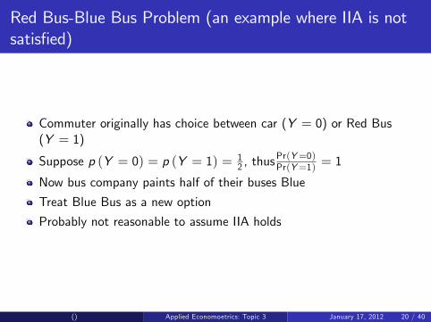
Red Bus-Blue Bus Problem (an example where IIA is notsatis�ed)

Commuter originally has choice between car (Y = 0) or Red Bus(Y = 1)

Suppose p (Y = 0) = p (Y = 1) = 12 , thus

Pr(Y=0)Pr(Y=1) = 1

Now bus company paints half of their buses Blue

Treat Blue Bus as a new option

Probably not reasonable to assume IIA holds


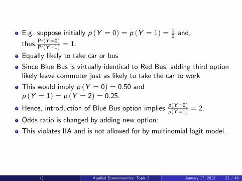
E.g. suppose initially p (Y = 0) = p (Y = 1) = 12 and,

thus,Pr(Y=0)Pr(Y=1) = 1.

Equally likely to take car or bus

Since Blue Bus is virtually identical to Red Bus, adding third optionlikely leave commuter just as likely to take the car to work

This would imply p (Y = 0) = 0.50 andp (Y = 1) = p (Y = 2) = 0.25.

Hence, introduction of Blue Bus option implies p(Y=0)p(Y=1) = 2.

Odds ratio is changed by adding new option:

This violates IIA and is not allowed for by multinomial logit model.


Is IIA reasonable or not?

Depends on your empirical application.

Sometimes it is reasonable, but other times not.

Note: there are extensions of multinomial logit models (not covered inthis course) that do not have restrictive IIA property:

Nested logit model and mixed logit model are two such extensions


Estimation of Multinomial Choice Models

We will not describe in detail estimation and testing with multinomialchoice models.

Maximum likelihood methods are used

Gretl will estimate them

Provide point estimates of coe¢ cients, P-values for telling whethercoe¢ cients are signi�cant

Various predicted probabilities and marginal e¤ects.

We will see how this is done in the computer session


Interpretation of Empirical Results in Multinomial ChoiceModelsMultinomial Logit

Use Empirical Example 1 (cracker data set)

N = 136 households

Each chooses between four brands of crackers: Sunshine, Keebler,Nabisco and Private label

We select �Private label� as the benchmark alternative

Remember: model utility di¤erence relative to choice 0


Hence, multinomial logit model has three equations: the �rst basedon utility di¤erence between Sunshine and Private label crackers, etc.

All equations include intercept and price of all four brands of crackersas explanatory variables.

Note: be careful with respect points made on: �Warning of IssuesConcerning Explanatory Variables�

This example has explanatory variables which di¤er across alternativesand three equations with di¤erent coe¢ cients

This is not quite the same as the models in Gujarati (chapter 9).


Interpretation of Multinomial Logit Results

Results in Table 9.3 (next 2 slides)

Note: three separate sets of regression results (in the panels of thetable labelled Sunshine, Keebler and Nabisco, respectively).

Like logit, hard to interpret size of the coe¢ cients in multinomial logit

But sign of any coe¢ cient can provide some information.

Coe¢ cients interpreted as marginal e¤ects relating to utilitydi¤erences

Positive coe¢ cient in equation j means explanatory variable haspositive e¤ect on utility di¤erence

If this utility di¤erence increases then individual more likely to choosealternative j relative to the benchmark choice.

Negative coe¢ cient make you less likely to choose option j


Table 9.3: Multinomial Logit Results for Cracker Data

MeanP-val forβji = 0

95% con�denceinterval

Sunshineα1 �10.06 0.15 [�23.59, 3.46]β11 �7.98 0.01 [�13.78,�2.20]β12 12.39 0.04 [0.77, 24.02]β13 0.37 0.91 [�5.83, 6.57]β14 4.83 0.36 [�5.54, 15.20]

Keeblerα2 �2.53 0.73 [�16.90, 11.85]β21 �3.10 0.30 [�9.01, 2.81]β22 �0.60 0.92 [�12.99, 2.81]β23 1.15 0.70 [�4.67, 6.97]β24 5.33 0.25 [�3.66, 14.32]


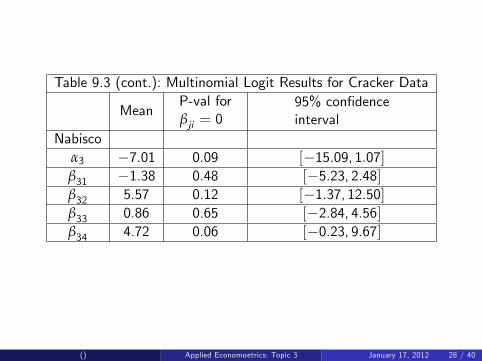
Table 9.3 (cont.): Multinomial Logit Results for Cracker Data

MeanP-val forβji = 0

95% con�denceinterval

Nabiscoα3 �7.01 0.09 [�15.09, 1.07]β31 �1.38 0.48 [�5.23, 2.48]β32 5.57 0.12 [�1.37, 12.50]β33 0.86 0.65 [�2.84, 4.56]β34 4.72 0.06 [�0.23, 9.67]


Interpreting Multinomial Logit Coe¢ cients (cont.)

Example: estimate of β11 is negative (�7.98)β11 is from Sunshine crackers equation

Utility di¤erence between Sunshine and Private label crackers is thedependent variable

β11 is coe¢ cient on explanatory variable �Price of SunshineCrackers�.

Interpretation: �if price of Sunshine crackers increases (holding theprice of other crackers constant), then the probability of choosingSunshine crackers over Private label crackers will fall�.

Sensible result (i.e. if the price of a good increases, consumers areless likely to buy it).

P-value for β11 says this coe¢ cient is signi�cant

Many other coe¢ cients are statistically insigni�cant


With logit model we used the odds ratio.

With multinomial logit, de�ne odds ratios for each option relative tothe benchmark option:

Pr (Yi = j)Pr (Yi = 0)

With logit, we said β can be interpreted as a marginal e¤ect in termsof the log odds ratio


Another thing to do: calculate predicted probability of choosing eachalternative for an individual with a speci�ed set of characteristics

Yet another: calculate the probability that each individual will chooseeach option

I.e. calculate Pr (Yi = j) for i = 1, ..,N and j = 0, .., J

Note: we have N = 136 individuals and four options: hence 544di¤erent Pr (Yi = j).

One thing you can do is present summary statistics of these 544probabilities.

This is done in Table 9.4.


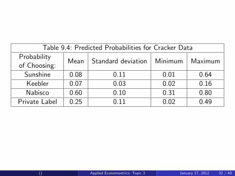
Table 9.4: Predicted Probabilities for Cracker DataProbabilityof Choosing:

Mean Standard deviation Minimum Maximum

Sunshine 0.08 0.11 0.01 0.64Keebler 0.07 0.03 0.02 0.16Nabisco 0.60 0.10 0.31 0.80

Private Label 0.25 0.11 0.02 0.49


Table 9.4 tells us things like:

Nabisco is the most popular brand

There is one individual about whom we can say �individual is 80%sure to choose Nabisco�

But nothing higher than 80% for any choice (lots of uncertainty inthis data set)

Results for the multinomial probit model are very similar so we willnot present them

Interpretation is as in probit, only now we have 3 equations


The conditional logit model is a special case of multinomial logit

I thought about not covering it (since in a sense we have alreadycovered it above)

Also Gretl does not seem to do it

But many other textbooks, research papers and computer packagesuse conditional logit so I will explain here


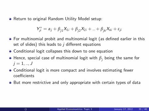
Return to original Random Utility Model setup:

Y �ji = αj + βj1X1i + βj2X2i + ..+ βjkXki + εji

For multinomial probit and multinomial logit (as de�ned earlier in thisset of slides) this leads to j di¤erent equations

Conditional logit collapses this down to one equation

Hence, special case of multinomial logit with βj being the same forj = 1, .., J

Conditional logit is more compact and involves estimating fewercoe¢ cients

But more restrictive and only appropriate with certain types of data


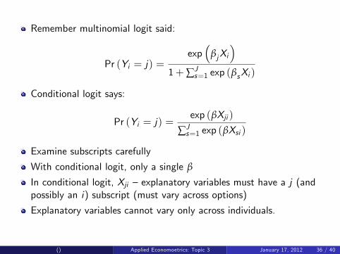
Remember multinomial logit said:

Pr (Yi = j) =exp

�βjXi

�1+∑J

s=1 exp (βsXi )

Conditional logit says:

Pr (Yi = j) =exp (βXji )

∑Js=1 exp (βXsi )

Examine subscripts carefully

With conditional logit, only a single β

In conditional logit, Xji �explanatory variables must have a j (andpossibly an i) subscript (must vary across options)

Explanatory variables cannot vary only across individuals.


To see why this is so consider an example:

One explanatory variable varies across choices (Xj ) and a second onevaries across individuals (Zi )

Conditional logit model would say:

Pr (Yi = j) =exp (β1Xij + β2Zi )

∑Js=1 exp (β1Xis + β2Zi )

But you can never estimate β2.

β2 disappears from Pr (Yi = j) and thus from the likelihood function� MLE not possible


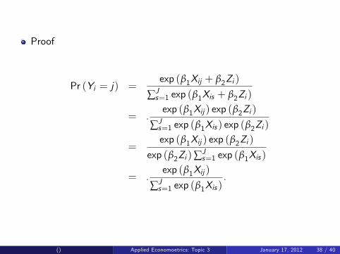
Proof

Pr (Yi = j) =exp (β1Xij + β2Zi )

∑Js=1 exp (β1Xis + β2Zi )

= .exp (β1Xij ) exp (β2Zi )

∑Js=1 exp (β1Xis ) exp (β2Zi )

=exp (β1Xij ) exp (β2Zi )

exp (β2Zi )∑Js=1 exp (β1Xis )

= .exp (β1Xij )

∑Js=1 exp (β1Xis )

.


Since conditional logit is special case of multinomial logit models, wewill not discuss estimation

Many computer packages (but not Gretl) can do MLE

As with all the qualitative choice models, it is hard directly tointerpret conditional logit coe¢ cients.

However, can estimate various predicted probabilities or variousmarginal e¤ects with respect to the probabilities.


Summary

Multinomial choice models are used when dependent variable ischoice between several options

Multinomial probit and multinomial logit are the most popularmultinomial choice models

If choice is between J + 1 options, both will have J equations

Conditional logit is a special case of multinomial logit with only 1equation

Maximum likelihood estimation is the most common way ofestimating all these models

Explanatory variables can be characteristics of the options or theindividuals (or both) and can lead to di¤erent models (so pay carefulattention

Care must be taken with interpretation of coe¢ cients/marginal e¤ects


Multinomial Choice Models -...

Documents

Transcript of Multinomial Choice Models -...