Multinational Firms, FDI Flows and Imperfect Capital

Markets

Pol Antràs, Mihir A. Desai, and C. Fritz Foley∗

December 5, 2006

Abstract

This paper examines how costly financial contracting and weak investor protection influ-

ence cross-border operational, financing and investment decisions of multinational firms. We

develop a model in which product developers have a comparative advantage in monitoring the

deployment of their technology abroad. The paper demonstrates that when firms want to

exploit technologies abroad, multinational firm (MNC) activity and foreign direct investment

(FDI) flows arise endogenously when monitoring is nonverifiable and financial frictions exist.

The mechanism generating MNC activity is not the risk of technological expropriation by local

partners but the demands of external funders who require MNC participation to ensure value

maximization by local entrepreneurs. The model demonstrates that weak investor protections

limit the scale of multinational firm activity, increase the reliance on FDI flows and alter the

decision to deploy technology through FDI as opposed to arm’s length licensing. Several dis-

tinctive predictions for the impact of weak investor protection on MNC activity and FDI flows

are tested and confirmed using firm-level data.

∗Harvard University and NBER; Harvard Business School and NBER; Harvard Business School and NBER, respec-tively. The statistical analysis of firm-level data on U.S. multinational companies was conducted at the InternationalInvestment Division, Bureau of Economic Analysis, U.S. Department of Commerce under arrangements that maintainlegal confidentiality requirements. The views expressed are those of the authors and do not reflect official positionsof the U.S. Department of Commerce. The authors thank seminar participants at MIT, the NBER ITI programmeeting, Oxford, UC Berkeley, UC Boulder, Universidad de Vigo, Universitat Pompeu Fabra, the New York Fed,and the World Bank for helpful suggestions. Davin Chor provided excellent research assistance.

1 Introduction

Firms globalizing their operations, and the associated capital flows, have become a major feature of

the world economy. These cross-border activities and capital flows span institutional settings with

varying investor protections and levels of capital market development. While the importance of

institutional heterogeneity in dictating economic outcomes has been emphasized, existing analyses

typically ignore the global firms and the capital flows that are now commonplace. Investigating

how global firms make operational and financing decisions in a world of heterogenous institutions

promises to provide a novel perspective on observed patterns of flows and firm activity.

This paper develops and tests a model of the operational and financial decisions of firms as

they exploit their technologies in countries with differing levels of investor protections. The model

demonstrates that multinational firm (MNC) activity and foreign direct investment (FDI) arise

endogenously in settings characterized by financial frictions. Furthermore, the model generates

several predictions regarding the use of arm’s length licensing to transfer technology, the degree to

which multinational firm activity is financed by capital flows, the extent to which multinationals

take ownership in foreign projects, and the scale of operations abroad. These predictions are tested

using firm-level data on U.S. multinational firms.

The model considers the problem of a firm (which we interpret as the parent firm of a multina-

tional corporation) seeking to deploy a proprietary technology abroad with the help of a local (or

host-country) entrepreneur. The central premise of the model is that the parent firm, as developer

of the technology, has a comparative advantage in monitoring how its technology is exploited and

can uniquely identify if local entrepreneurs are pursuing value maximization. A set of external in-

vestors are attractive sources of finance for the exploitation of the technology abroad because they

face a lower opportunity cost of capital than that faced by the entrepreneur and the parent firm. In

order to convince external funders to supply capital, entrepreneurs need to give financial claims on

the project to parent firms to ensure that they provide monitoring when monitoring is unverifiable,

thus mitigating managerial misbehavior (e.g., theft) by entrepreneurs. The concern over managerial

misbehavior, and the requirement for parent firm participation, is particularly acute when investor

protections are weak.

The characterization of multinational firms as developers of technologies has long been central

to models explaining multinational firm activity. In contrast to those models that emphasize the

risk of technology expropriation, the model in this paper emphasizes financial frictions, a cruder

form of managerial opportunism and the role of external funders. As such, while technology is

central to these other models and the model in this paper, the mechanism generating multinational

firm activity is entirely distinct. Our emphasis on monitoring builds on the theory presented in

Holmstrom and Tirole (1997) which captures how monitoring is critical to understanding financial

intermediation.

In deriving our theoretical results, we find it useful to first develop a benchmark in which moni-

toring is verifiable. In this setting, we show that when the developer of technology wants to deploy

its technology abroad, it chooses to license this technology to the host country entrepreneur who

1

obtains financing from external investors. Under these circumstances, the entrepreneur can exploit

technology without giving a financial claim on the project to the developer, who simply obtains

a flat fee for the use of its proprietary technology. Nevertheless, when monitoring is verifiable,

weak investor protections still limit the scale of projects because these environments require more

monitoring and this inflates the marginal cost of production.

When monitoring is nonverifiable, capital flows and multinational ownership of assets abroad

arise endogenously to align the incentives of the inventors of technology and the entrepreneurs in

host economies. In this setting, we show that an optimal contract calls for the developer of the

technology (the parent firm) to take an equity share on the return of the project and may also

call for the parent firm to provide funds for investment, even though external investors are more

efficient sources of financing.1

The case of nonverifiable monitoring delivers several novel predictions about the nature of

FDI and patterns of multinational firm activity. First, the model predicts that technology will

be exploited through unrelated party licensing rather than through affiliate activity in countries

where investor protections are stronger. Second, the share of activity abroad financed by capital

flows from the multinational parent will be decreasing in the quality of investor protections in host

economies. Third, ownership shares by multinational parents will also be decreasing in the quality

of investor protections in host economies. These predictions reflect the fact that monitoring by the

developer of the technology is more critical in settings where investor protections are weaker. The

model also predicts that the scale of activity based on multinational technologies in host countries

will be an increasing function of the quality of the institutional environment. Better capital market

conditions reduce the need for monitoring and therefore allow for a larger scale of activity.

We test these predictions using the most comprehensive available data on the activities of U.S.

multinational firms. These data provide details on the world wide operations of U.S. multinationals

and include measures of parental ownership, financing and operational decisions. These data enable

the use of parent-year fixed effects that implicitly control for a variety of unobserved attributes.

The analysis indicates that the likelihood of using arm’s length licensing to serve a foreign

market increases with measures of investor protections, as suggested by the model. The predictions

on parent financing and ownership decisions are also confirmed to be a function of the quality of

investor protections and the depth of capital markets. The model also suggests that these effects

should be most pronounced for technologically advanced firms because these firms are most likely

to be able to provide valuable monitoring services. The empirical evidence indicates a differential

effect for these kinds of firms.

Settings where ownership restrictions are liberalized provide an opportunity to test the final

prediction of the model. The model implies that these liberalizations should have a particularly

large effect on multinational affiliate activity in countries with weak investor protections because,

in those countries, ownership restrictions limit multinational firm activity the most. Our empirical

1Following Holmstrom and Tirole (1997), in our model contracting is “complete” in the sense that we solve forthe optimal contract subject to explicit information frictions. This is in contrast to a large incomplete-contractingliterature in corporate finance.

2

analysis confirms that affiliate activity grows fastest after liberalizations in countries with weaker

investor protections.

This paper extends the large and growing literature on the effects of investor protection and

capital market development on economic outcomes to an open economy setting where firms make

operational and financial decisions across borders. La Porta, Lopez-de-Silanes, Shleifer and Vishny

(1997, 1998) relate investor protections to the concentration of ownership and the depth of capital

markets and a large literature, including Rajan and Zingales (1998), Wurgler (2000), and Acemoglu,

Johnson and Mitton (2005), has shown that financial market conditions influence firm investment

behavior and industrial structure.

By exclusively emphasizing firms with local investment and financing, this literature has ne-

glected how cross-border, intrafirm activity responds to institutional variations. The open economy

dimensions of institutional variations have been explored, but only in the context of cross-border

lending as in Gertler and Rogoff (1990), Boyd and Smith (1997) and Shleifer and Wolfenzon (2002).2

The model in this paper demonstrates how both multinational activity and capital flows respond

to heterogeneity in institutional settings. In short, we show that weak financial institutions de-

crease the scale of multinational firm activity but simultaneously increase the reliance on capital

flows from the parent. As such, observed patterns of capital flows reflect these two distinct and

contradictory effects. The empirical investigations of micro-data provided in the paper indicate

that both effects are operative.

By jointly considering the determinants of MNC activities and the flows of capital that support

these activities, the paper also links two literatures—the international trade literature on multina-

tionals and the macroeconomic literature on capital flows. Industrial organization and international

trade scholars characterize multinationals as having proprietary assets and emphasize the role of

market imperfections like transport costs and market power in determining patterns of multinational

activity. Recent work on multinational firms investigates “horizontal” or “vertical” motivations3

for foreign direct investment and explores why alternative productive arrangements like whole own-

ership of foreign affiliates, joint ventures, exports or arm’s length contracts are employed.4

Such analyses of multinational firm activity typically do not consider associated capital flows.5

2Gertler and Rogoff (1990) show how arms-length lending to entrepreneurs in poor countries is limited by theirinability to pledge large amounts of their own wealth. This insight is embedded into a multinational firm’s productiondecisions in the model presented here. Our setup also relates to Shleifer and Wolfenzon (2002), who study the interplaybetween investor protection and equity markets. In contrast, Kraay et al. (2005) emphasize the role of sovereign riskin shaping the structure of world capital flows.

3The horizontal FDI view represents FDI as the replication of capacity in multiple locations in response to factorssuch as trade costs, as in Markusen (1984), Brainard (1997), Markusen and Venables (2000), and Helpman, Melitzand Yeaple (2004). The vertical FDI view represents FDI as the geographic distribution of production globally inresponse to the opportunities afforded by different markets, as in Helpman (1984) and Yeaple (2003). Caves (1996)and Markusen (2002) provide particularly useful overviews of this literature.

4Antràs (2003, 2005), Antràs and Helpman (2004), Desai, Foley and Hines (2004), Ethier and Markusen (1996),Feenstra and Hanson (2005), and Grossman and Helpman (2004) analyze the determinants of alternative foreignproduction arrangements.

5Several studies linking levels of MNC activity and FDI flows are worth noting. First, high frequency changes inFDI capital flows have been linked to relative wealth levels through real exchange rate movements (as in Froot andStein (1991) and Blonigen (1997)), broader measures of stock market wealth (as in Klein and Rosengren (1994) and

3

Research on capital flows typically abstracts from firm activity and has focused on the paradox

posed by Lucas (1990) of limited capital flows from rich to poor countries in the face of large

presumed rate of return differentials. While Lucas (1990) emphasizes human-capital externalities

to help explain this paradox, Reinhart and Rogoff (2004) review subsequent research on aggregate

capital flows and conclude that credit market conditions and political risk play significant roles.

By examining firm behavior in a setting of hetergenous institutional setting, this paper attempts

to unify an investigation of multinational firm activity and FDI flows.

The rest of the paper is organized as follows. Section 2 lays out the model and discusses the case

of fully verifiable monitoring, extends the model to settings of nonverifiable monitoring and then

generates several predictions related to the model. Section 3 provides details on the data employed

in the analysis. Section 4 presents the results of the analysis and Section 5 concludes.

2 Theoretical Framework

We begin this section by describing a simple partial equilibrium model of financing that builds on

and extends the work of Holmstrom and Tirole (1997).6 We later illustrate how the model is able to

generate both multinational activity as well as foreign direct investment flows. Finally, we explore

some firm-level empirical predictions that emerge from the model.

2.1 A Simple Model of Financial Contracting

Environment

We consider the problem of an agent — an inventor — who is endowed with an amount W of

financial wealth and the technology or knowledge to produce a differentiated good. Consumers

in two countries, Home and Foreign, derive utility from consuming this differentiated good.7 The

good, however, is prohibitively costly to trade and thus servicing a particular market requires

setting up a production facility in that country. The inventor is located at Home and cannot fully

control production in Foreign. Servicing that market thus requires contracting with a foreign agent

— an entrepreneur — to manage production there. We assume that entrepreneurs are endowedwith no financial wealth and their outside option is normalized to 0. There also exists a continuum

Baker, Foley and Wurgler (2005)) and to credit market conditions (as in Klein, Peek and Rosengren (2002)). Second,multinational firms have also been shown to opportunistically employ internal capital markets in weak institutionalenvironments (as in Desai, Foley and Hines (2004b)) and during currency crises (as in Aguiar and Gopinath (2005)and Desai, Foley and Forbes (2005)). These papers emphasize how heterogeneity in access to capital can interactwith multinational firm production decisions. Marin and Schnitzer (2004) also study the financing decisions ofmultinational firms in a model that stresses managerial incentives. Their model however takes the existence ofmultinational firms as given and considers an incomplete-contracting setup in contrast to our complete-contractingsetup. The predictions from their model are quite distinct (and typically contradictory) to the ones we develop hereand show to be supported by U.S. data.

6Our model generalizes the setup in Holmstrom and Tirole (1997) by allowing for diminishing returns to investmentand for variable monitoring levels. The scope of the two papers is also very distinct: they studied the monitoringrole of banks in a closed-economy model, while our focus is on multinational firms.

7 In the Appendix, we develop a multi-country version of the model.

4

of infinitessimal external investors in Foreign that have access to a technology that gives them a

gross rate of return equal to 1 on their wealth. All parties are risk neutral and are protected by

limited liability. There are three periods, a date 0 contracting stage, a date 1 investment stage,

and a date 2 production/consumption stage.

Consumer Preferences and Technology

In the main text, we focus on describing production and financing decisions in the Foreign market.

For that purpose, we assume that preferences and technology at Home are such that at date 2 the

inventor obtains a constant gross return β > 1 for each unit of wealth he invests in production

at Home at date 1. We refer to this gross return as the inventor’s shadow value of cash. In the

Appendix, the value of β is endogenously derived in a multi-country version of the model where

consumer preferences, technology and financial contracting in all countries are fully specified.

We assume that Foreign preferences are such that cash flows or profits obtained from the sale

of the differentiated good in Foreign can be expressed as a strictly increasing and concave function

of the quantity produced, i.e, R (q), with R0 (q) > 0 and R00 (q) ≤ 0. We also assume the standardconditions R (0) = 0, limq→0R0 (q) = +∞, and limq→∞R0 (q) = 0. These properties of R (q) can be

derived from preferences featuring a constant (and higher-than-one) elasticity of substitution across

(a continuum of) differentiated goods produced by different firms. In such case, the elasticity of

R (q) with respect to q is constant and given by a parameter α ∈ (0, 1).Foreign production is managed by the foreign entrepreneur, who at date 1 can privately choose

to behave or misbehave. When the manager behaves, the project performs with probability pH , in

the sense that when an amount x is invested at date 1, project cash flows at date 2 are equal to R (x)

with probability pH and 0 otherwise.8 When the manager misbehaves, the project performs with

a lower probability pL < pH and expected cash flows are pLR (x). We assume, that the manager

obtains a private benefit from misbehaving and that this private benefit is proportional to the return

of the project, i.e., BR (x). As described below, we will relate this private benefit to the stage of

financial development in Foreign as well as to the extent to which the entrepreneur is monitored.

The idea is that countries with better investor protections tend to enforce laws that limit the ability

of managers to divert funds from the firm or to enjoy private benefits or perquisites.9

When investor protections are weak, monitoring by third agents is helpful in reducing the extent

to which managers are able to divert funds or enjoy private benefits. Following Holmstrom and

Tirole (1997), we introduce a monitoring technology that reduces the private benefit of the foreign

entrepreneur when he misbehaves. It is natural to assume that the inventor has a comparative

advantage in monitoring the behavior of the foreign entrepreneur because the inventor is particularly

well informed about the mapping between managerial effort and output inherent in the production

of that good.10 We capture this in a stark way by assuming that no other agent in the economy

8This assumes that, when the project succeeds, each unit invested results in a unit of output (q = x), while whenthe project fails, output is zero (q = 0).

9See Tirole (2006, p. 359) for more on this interpretation.10An alternative way to interpret monitoring is as follows. Suppose that the foreign entrepreneur can produce

5

can productively monitor the foreign entrepreneur. Conversely, when the inventor incurs an effort

cost CR (x) in monitoring at date 1, the private benefit for the local entrepreneur is multiplied by

a factor δ (C), with δ0 (C) < 0, δ00 (C) > 0, δ (0) = δ, limC→∞ δ (C) = 0, limC→0 δ0 (C) = −∞, and

limC→∞ δ0 (C) = 0.11

The scope of private benefits is related to the level of investor protection of the host country by

an index γ ∈ (0, 1). In particular, we specify that

B (C; γ) = (1− γ) δ (C) . (1)

Note that this formulation implies that ∂B (·) /∂γ < 0, ∂B (·) /∂C < 0, and ∂2B (·) /∂C∂γ =−δ0 (C) > 0. This formulation captures the intuition that the scope for private benefits is decreasingin both investor protection and monitoring, and that monitoring has a relatively larger effect on

private benefits in countries with poor legal protection of investors.

Contracting

We consider optimal contracting between three sets of agents: the inventor, the foreign entrepreneur

and foreign external investors. At date 0, the inventor and the foreign entrepreneur negotiate

a contract that stipulates the terms under which the entrepreneur will exploit the technology

developed by the inventor. This contract includes a date-0 transfer P from the entrepreneur to

the inventor, as well as the agents’ date-2 payoffs contingent on the return of the project.12 When

P > 0, the date-0 payment can be thought of as the price or royalties paid for the use of the

technology, which the inventor can invest in the Home market at date 1. When P < 0, we can

think of the inventor as cofinancing the project in the Foreign country. The contract between the

inventor and the entrepreneur also stipulates the date-1 scale of investment x, while the managerial

and monitoring efforts of the entrepreneur and inventor, respectively, are unverifiable and thus

cannot be part of the contract. To build intuition, we consider in Section 2.2 the case in which

monitoring is verifiable.

Also at date 0, the foreign entrepreneur and external investors sign a financial contract under

which the entrepreneur borrows an amount E from the external investors at date 0 in return for a

date-2 payment contingent on the return of the project.

We consider an optimal contract from the point of view of the inventor and allow the contract

between the inventor and the entrepreneur to stipulate the terms of the financial contract between

the entrepreneur and foreign external investors. We rule out “direct” financial contracts between

the good under a variety (a continuum, actually) of potential techniques indexed by z ∈ [0, B]. Technique 0 entailsa probability of success equal to pH and a zero private benefit. All techniques with z > 0 are associated witha probability of success equal to pL and a private benefit equal to z. Clearly, all techniques with z ∈ (0, B) aredominated from the point of view of the foreign entrepreneur, who will thus effectively (privately) choose either z = 0or z = B, as assumed in the main text. Under this interpretation, we can think of monitoring as simply makingcertain high-private benefit projects not available to the entrepreneur, i.e., reducing the upper bound of [0, B].11These conditions are sufficient to ensure that the optimal contract is unique and satisfies the second-order con-

ditions.12For simplicity, we assume that the inventor’s date-1 return in its Home market is not pleadgeable in Foreign.

6

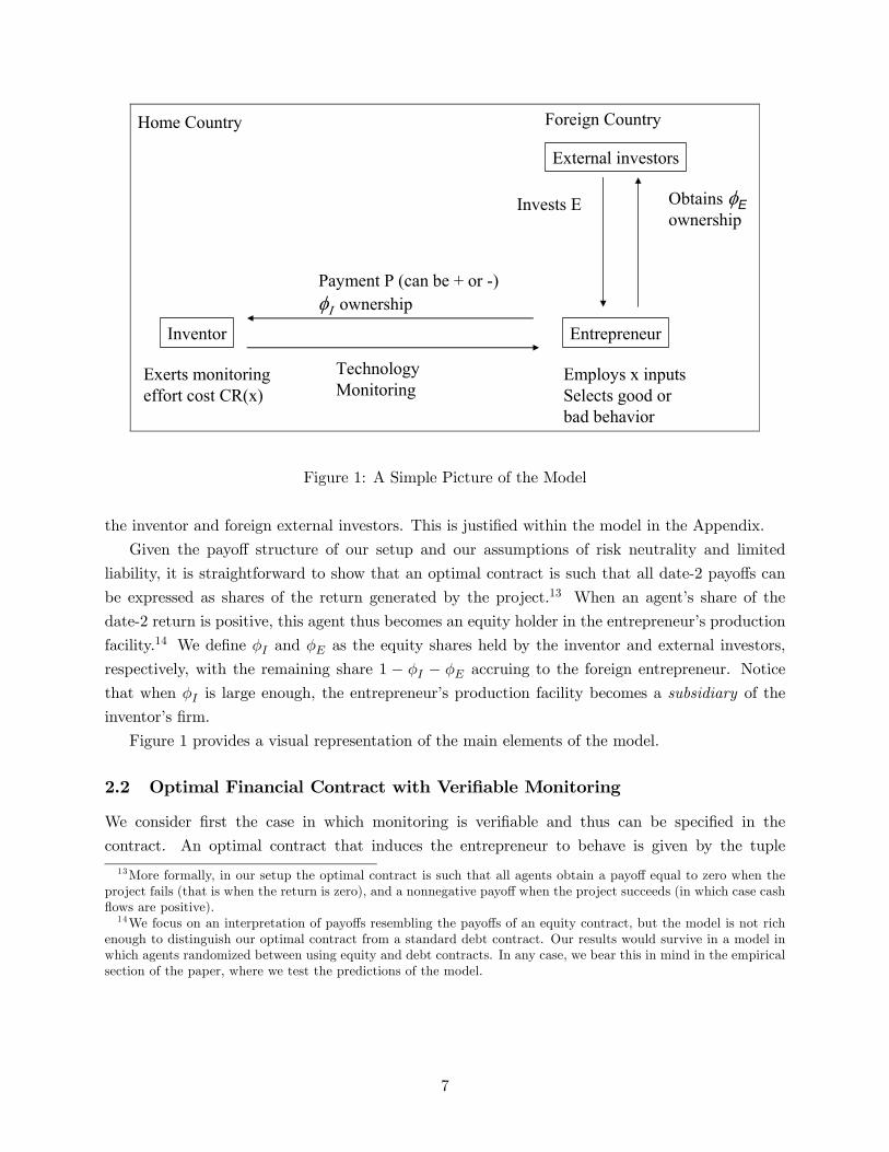
External investors

Foreign Country

Inventor

Home Country

Entrepreneur

TechnologyMonitoring

Payment P (can be + or -)φΙ ownership

Invests E Obtains φEownership

Employs x inputsSelects good orbad behavior

Exerts monitoring effort cost CR(x)

Figure 1: A Simple Picture of the Model

the inventor and foreign external investors. This is justified within the model in the Appendix.

Given the payoff structure of our setup and our assumptions of risk neutrality and limited

liability, it is straightforward to show that an optimal contract is such that all date-2 payoffs can

be expressed as shares of the return generated by the project.13 When an agent’s share of the

date-2 return is positive, this agent thus becomes an equity holder in the entrepreneur’s production

facility.14 We define φI and φE as the equity shares held by the inventor and external investors,

respectively, with the remaining share 1 − φI − φE accruing to the foreign entrepreneur. Notice

that when φI is large enough, the entrepreneur’s production facility becomes a subsidiary of the

inventor’s firm.

Figure 1 provides a visual representation of the main elements of the model.

2.2 Optimal Financial Contract with Verifiable Monitoring

We consider first the case in which monitoring is verifiable and thus can be specified in the

contract. An optimal contract that induces the entrepreneur to behave is given by the tuple

13More formally, in our setup the optimal contract is such that all agents obtain a payoff equal to zero when theproject fails (that is when the return is zero), and a nonnegative payoff when the project succeeds (in which case cashflows are positive).14We focus on an interpretation of payoffs resembling the payoffs of an equity contract, but the model is not rich

enough to distinguish our optimal contract from a standard debt contract. Our results would survive in a model inwhich agents randomized between using equity and debt contracts. In any case, we bear this in mind in the empiricalsection of the paper, where we test the predictions of the model.

7

nP , φI , x, φE, E, C

othat solves the following program:

maxP,φI ,x,φE ,E,C

ΠI = φIpHR (x) + (W + P )β − CR (x)

s.t. x ≤ E − P (i)

pHφER (x) ≥ E (ii)

pH (1− φE − φI)R (x) ≥ 0 (iii)

(pH − pL) (1− φE − φI)R (x) ≥ (1− γ) δ (C)R (x) (iv)

φI ≥ 0 (v)

(P1)

The objective function represents the payoff of the inventor. The first term represents the

inventor’s dividends from the expected cash flows of the foreign production facility. The second

term represents the gross return from investing his wealth W plus the date-0 transfer P in the

Home market. The last term represents the monitoring costs.

The first constraint is a financing constraint. Since the local entrepreneur has no wealth, his

ability to invest at date 1 is limited by whatever is left from the external investors’ financing E after

satisfying the payment P to the inventor. The second inequality is the participation constraint of

external investors, who need to earn at least an expected gross return on their investments equal to

1. Similarly, the third inequality is the participation constraint of the foreign entrepreneur, given

his zero outside option. The fourth inequality is the foreign entrepreneur’s incentive compatibility

constraint. This presumes that it is in the interest of the inventor to design a contract in a way that

induces the foreign entrepreneur to behave.15 The final inequality is a non-negativity constraint on

the share of equity held by the inventor.16

In the program above, constraint (iii) will never bind. Intuitively, as is standard in incomplete

information problems, the incentive compatibility constraint of the entrepreneur demands that this

agent obtains some informational rents in equilibrium, and thus his participation constraint is slack.

The other four constraints will bind in equilibrium. This is intuitive for the financing constraint

(i), the participation constraint of investors (ii), and the incentive compatibility constraint (iv). In

addition, the fact that constraint (v) binds immediately implies that the equilibrium equity share

of the inventor satisfies

φI = 0, (2)

and thus the overall payoff of the inventor is not contingent on the outcome of the project. The in-

tuition for this result is that with verifiable monitoring, equity shares are not an optimal mechanism

for transferring utility from the entrepreneur to the inventor. It may appear that a positive φI is

attractive because it reduces the required lump-sum price for the technology P and thus encourages

investment. However, inspection of constraint (iii) reveals that a larger φI decreases the ability of

the entrepreneur to borrow from external investors, as it reduces his pleadgeable income. Overall,

one can show that whether utility is transferred through an equity share or a date-0 lump-sum

15Below we derive conditions under which this choice is optimal.16We assume throughout that W is large enough to ensure that W + P ≥ 0 in equilibrium.

8

payment has no effect on the scale of the project. In addition, it is clear from the objective function

that the inventor strictly prefers a date-0 lump-sum transfer since it can use these funds in his

domestic investments and obtain a gross rate of return β > 1 on them. Hence, φI = 0 is optimal.

Manipulation of the first-order conditions of the problem also delivers the unique optimal

amount of monitoring, which is implicitly given by:

−δ0³C´=

pH − pL(1− γ)βpH

. (3)

Because δ00 (·) > 0, we find that monitoring C is relatively higher when the entrepreneur resides

in a country with a lower level of investor protection (low γ) or when the inventor has a relatively

high shadow value of cash (high β). Both cases correspond to situations in which the entrepreneur

is relatively more constrained, so the marginal benefit of monitoring is especially high in those

cases.

With the equilibrium value for monitoring, the remaining values for the optimal contract can

easily be derived. In particular, straightforward manipulation of the first order conditions delivers

(see Appendix):

R0 (x) =1

pH

µ1− (1−γ)δ(C)

pH−pL − CβpH

¶ . (4)

Making use of equation (3) and the concavity of R (x), one can show (see Appendix) that x is

necessarily increasing in γ, that is, output and cash flows are higher in host countries with better

investor protections. In the limit in which γ → 1, we find that C → 0 and R0 (x) = 1/pH , which

corresponds to the first-best level of investment. Similarly, we can show that output and cash flows

are strictly increasing in β, the shadow value of cash of the inventor. Intuitively, the larger is β,

the larger is the incentive to use monitoring to reduce inefficiencies and generate a larger P that

can be invested in the domestic economy.

Using constraints (i), (ii), and (iii), one can obtain the equilibrium values of φE and E in terms

of C and x :

φE = 1−(1− γ) δ

³C´

pH − pL(5)

E = pH φER (x) . (6)

In addition, straightforward manipulation delivers

P =

µR (x)

R0 (x) x− 1¶x+

1

βCR (x) > 0, (7)

where the sign follows from R (x) /x > R0 (x) > 1 given the concavity of R (x) and R (0) = 0.

In sum, the optimal contract is such that the inventor does not take a positive stake in the

entrepreneurs’ production facility and simply receives a positive lump-sum fee for the exploitation

9

of the technology. Finally, we can compute the net payoff of the inventor, which is given by

ΠI = βW + β

µR (x)

R0 (x) x− 1¶x.

We summarize the main results in this section in the following proposition (see the Appendix

for a formal proof):

Proposition 1 (Verifiable Monitoring) There exist a unique tuplenP , φI , x, φE, E, C

othat

solves program (P1). Furthermore, an optimal contract that induces the entrepreneur to behave is

characterized by equations (2)-(7) and is such that:

1. The inventor does not take an equity stake in the local entrepreneur’s production facility

(φI = 0).

2. The inventor receives a positive lump-sum transfer (P > 0) for the use of the technology.

3. Output and cash flows are increasing in investor protection in Foreign (γ) and in the inventor’s

shadow value of cash (β).

4. Monitoring is decreasing in γ and increasing in β.

Proof. See Appendix.

So far we have ignored the possibility that the inventor does not induce the entrepreneur to

behave. In the Appendix, we show that the inventor in that case would obtain a payoff equal to

ΠLI = βW + β

ÃR¡xL¢

R0 (xL) xL− 1!xL

where xL is implicitly defined by

R0¡xL¢=1

pL. (8)

It is thus clear that as long as x > xL, the contract described in Proposition 1 is the optimal

contract. Given that when γ → 1, R0 (x) → 1/pH < 1/pL = R0¡xL¢, good behavior is necessarily

induced whenever γ is sufficiently high.

2.3 Nonverifiable Monitoring and the Emergence of Foreign Direct Investment

We next consider the case in which monitoring is not verifiable and thus cannot be specified in

the contract. Specifically, we consider the case in which, at date 1, the inventor privately sets the

level of monitoring C, after which the entrepreneur observes his private benefit from misbehaving

B³C´and decides whether to behave or misbehave. In this case, the contract has to be such that

the inventor finds it privately optimal to exert monitoring effort.

10

It is straightforward to see that the contract specified in the previous section does not accomplish

this. In particular, notice that whenever φI = 0, the payoff of the inventor is independent of

the behavior of the entrepreneur, and thus the inventor will not have any incentive to monitor

the entrepreneur at date 1. Hence, given the contract in Proposition 1, the inventor would set

C = 0, which would of course imply that the entrepreneur’s private benefit from misbehaving is

limC→0B (C) = (1− γ) δ, and for large enough δ, his incentive compatibility is violated. In sum,

as long as the inventor’s payoff is not contingent on the return of the investment, the inventor will

not exert a positive monitoring effort and, for large enough δ, the entrepreneur misbehaves.

We next show that the inventor may improve upon this outcome by modifying the previous

contract in a way that induces good behavior on the part of the entrepreneur. This requires the

inventor’s equity stake to be positive. It is still the case, however, that the inventor has an incen-

tive to set the minimum monitoring level C such that the entrepreneur’s incentive compatibility

constraint is satisfied. This implies that this monitoring cost is implicitly given by:

(pH − pL) (1− φE − φI) = (1− γ) δ³C´.

In order for this positive monitoring effort to be credible, the initial contract needs to satisfy the

following incentive compatibility constraint for the inventor:

φIpHR (x)− CR (x) ≥ φIpLR (x) .

This condition corresponds to the intuition that the inventor’s payoff should be higher when exerting

the positive monitoring level C than when not doing so.17

It follows from the above discussion that an optimal contract that induces the entrepreneur to

behave is now given by the tuplenP , φI , x, φE, E, C

othat solves the following program:18

maxP,φI ,x,φE ,E,C

ΠI = φIpHR (x) + (W + P )β − CR (x)

s.t. x ≤ E − P (i)

pHφER (x) ≥ E (ii)

pH (1− φE − φI)R (x) ≥ 0 (iii)

(pH − pL) (1− φE − φI)R (x) = (1− γ) δ (C)R (x) (iv)

(pH − pL)φIR (x) ≥ CR (x) (v’)

(P2)

This program is identical to (P1) except for the inclusion of the new incentive compatibility

constraint (v’) for the inventor.19 We show in the Appendix that it is again the case that, except

for constraint (iii), the remaining constraints all bind in an optimal contract. This immediately

17Our derivation of this IC constraint assumes that if the inventor deviates from C, it does so by setting C = 0,but this is without loss of generality because any other deviation C > 0 is dominated.18We again assume that W is high enough such that the constraint W + P ≥ 0 never binds.19To be precise, it differs also in the fact that the private choice of C ensures that (iv) will bind. But this is

immaterial since that constraint was binding in program (P1) as well.

11

implies that the solution to (P2) entails the inventor taking a positive equity stake in the project

undertaken by the foreign entrepreneur. In particular, from constraint (v’), we immediately obtain

φI =C

pH − pL, (9)

which will be positive as long as C is positive. In addition, the level of monitoring is now implicitly

given by the expression (see Appendix for details)

−δ0³C´=

βpH − pL(1− γ)βpH

. (10)

Direct comparison of (3) and (10) reveals that δ0³C´> δ0

³C´and thus C < C. In words, when

monitoring is nonverifiable, it is underprovided. Next, working with the first-order conditions of

program (P2), the level of output is implicitly given by:

R0 (x) =1

pH

µ1− (1−γ)δ(C)

pH−pL −³βpH−pLpH−pL

´C

βpH

¶ . (11)

As in the case with verifiable monitoring, whenever γ → 1, we have that C → 0 and x is set at the

first-best level implicitly defined by R0 (x) = 1/pH .

The terms of the financial contract with external investors are now given by:

φE = 1−(1− γ) δ

³C´

pH − pL− C

pH − pL(12)

E = pH φER (x) . (13)

Straightforward manipulation delivers an optimal lump-sum date-0 transfer equal to:

P =

µR (x)

R0 (x) x− 1¶x− pL

β (pH − pL)CR (x) . (14)

Comparing this initial lump-sum transfer with the result of verifiable monitoring, we note that,

provided that α (x) ≡ R (x) / (R0 (x)x) is nondecreasing in x, it will necessarily be the case that

P < P , and the initial transfer is lower with nonverifiable monitoring. As mentioned above,

when preferences feature a constant elasticity of substitution across a continuum of differentiated

goods produced by different firms, α (x) is in fact independent of x, and R (x) can be written as

R (x) = Axα, where A > 0 and α ∈ (0, 1). In such case, the initial lump-sum transfer can be

written as

P =

µ1− α

α

¶x− pL

β (pH − pL)CA (x)α .

Notice that the initial transfer payment is also not necessarily positive in this case. In particular,

given the concavity of R (x), if the optimal level of x is low enough, R (x) /x will be large, and P

12

will be negative.

To summarize, introducing the nonverifiability of monitoring transforms a transaction that has

the properties of a market transaction—the payment of a flat fee for the use of a technology— into

something that has the properties of foreign direct investment. When monitoring is nonverifiable, it

is optimal for the inventor to take an equity stake in the project and instead of charging a positive

price for the use of the technology, the inventor may now decide instead to cofinance the foreign

operations by setting a negative P at date 0. In sum, we have shown (see the Appendix for formal

proofs) that:

Proposition 2 (Nonverifiable Monitoring) There exist a unique tuplenP , φI , x, φE , E, C

othat solves program (P2). Furthermore, an optimal contract that induces the entrepreneur to

behave is characterized by equations (9)-(14) and is such that:

1. The inventor takes a positive equity stake in the local entrepreneur’s production facility

(φI > 0).

2. Depending on parameter values, the entrepreneur may receive a positive lump-sum transfer

(P > 0) for the use of the technology or it may instead cofinance the project via an initial

capital transfer (P < 0).

Proof. See Appendix.

Before moving to an analysis of the comparative statics, it is important to consider the possibility

that the inventor decides not to implement good behavior on the part of the foreign entrepreneur.

We show in the Appendix, that this is never optimal provided that x > xL, where xL is defined in

equation (8). Because as γ → 1, R0 (x) → 1/pH , we can conclude again that inducing the foreign

entrepreneur to behave is indeed optimal whenever γ is sufficiently high.

2.4 Comparative Statics: Firm-Level Empirical Predictions

In order to guide the empirical analysis, we outline the predictions that the model generates con-

cerning patterns of multinational firm activity and financing flows. This subsection highlights the

effects of investor protection γ in Foreign on: (i) the scale of activity; (ii) the extent of inventor

ownership; and (iii) the share of capital provided by the inventor. We also describe the effects

of the shadow value of cash β on all these objects. As our estimation employs parent-firm fixed

effects, we do not test these predictions about β.

As is clear from equations (9), (11) and (14), in order to understand the effects of γ and β on

the main observable components of the optimal contract, we first have to investigate the effect of

these parameters on the optimal amount of monitoring. Straightforward differentiation of equation

(10) together with the convexity of the function δ (·) produces the following result:

Lemma 1 The amount of monitoring C is decreasing in both investor protection γ in Foreign and

in the inventor’s shadow value of cash β.

13

Proof. See Appendix.

The effect of investor protection on monitoring is similar to the effect described in the case

of verifiable monitoring. Given our specification of the private benefit function B (·) in (1), themarginal benefit from monitoring is larger the less developed is the financial system in Foreign (the

lower is γ). Since the marginal cost of monitoring is independent of γ, in equilibrium C and γ are

negatively correlated.

The effect of the shadow value of cash β on monitoring is quite distinct from the case with

verifiable monitoring, where monitoring is increasing in β. The intuition for this divergence stems

from the fact that the incentive compatibility constraint of the inventor becomes tighter the larger

is the amount of monitoring in equilibrium. In particular, a higher level of monitoring requires a

larger equity share φI . This is costly because for β > 1, the inventor would like to receive a larger

share of the the foreign entrepreneur’s payments upfront. The larger is β, the higher is the shadow

cost of monitoring working through the incentive compatibility constraint, and the lower is the

optimal amount of monitoring.

Our theory has implications for the share of equity held by the inventor that relate closely to

the implications for monitoring. From equation (9), it is obvious that the share φI is proportional

to the level of monitoring and thus is affected by the parameters γ and β in the same way as

is monitoring. This simply reflects that equity shares emerge in our model as incentives for the

inventor to monitor the foreign entrepreneur. As a result, we can establish that:

Proposition 3 The share of equity held by the inventor is decreasing both in investor protectionγ in Foreign and in the inventor’s shadow value of cash β.

Proof. Proof in text.

An immediate corollary of this result is:

Corollary 1 Suppose that a transaction is recorded as an FDI transaction if φI ≥ φI and as a

licensing transaction if φI < φI . Then, there exist a threshold investor protection γ∗ ∈ [0, 1] overwhich the optimal contract entails licensing and under which the optimal contract entails FDI.

With these results at hand, differentiation of equation (11), which implicitly defines the equi-

librium level of x and R (x), yields the conclusion that:

Proposition 4 Output and cash flows in Foreign are increasing in investor protection γ in Foreignand decreasing in the inventor’s shadow value of cash β.

Proof. See Appendix.

The intuition for the effect of investor protection is straightforward. Despite the fact that the

inventor’s monitoring reduces financial frictions, both the foreign entrepreneur’s compensation, as

dictated by his incentive compatibility constraint (iv), and monitoring costs are increasing in the

14

scale of operation. In countries with worse financial institutions, the perceived marginal cost of

investment is therefore higher, thus reducing equilibrium levels of investment.

Finally, our model also generates predictions for the sources of financing of the foreign produc-

tion facility. To see this, focus on the case in which the date-0 payment P is actually negative

and can be interpreted as the inventor cofinancing Foreign activity. Define the amount of financing

provided by the inventor by F ≡ −P . The share of investment financed by the inventor is thengiven by

F

x=

pLβ (pH − pL)

CR (x)

x−µ1− α (x)

α (x)

¶,

where α (x) ≡ R (x) / (R0 (x) x). Notice that this expression is increasing in C. Furthermore, pro-

vided that α (x) does not increase in x too quickly, the ratio F /x is decreasing in x, due to the

concavity of R (·). It thus follows from Lemma 1 and Proposition 4 that:

Proposition 5 Provided that α (x) does not increase in x too quickly, the share of inventor fi-

nancing in total financing (F /x) is decreasing in investor protection γ.

Proof. Proof in text.

The intuition behind the result is that monitoring by inventors has a relatively high marginal

product in countries with weak financial institutions. To induce the inventor to monitor, the optimal

contract specifies a relatively “steeper” payment schedule, with a relatively higher contribution by

the inventor at date 0 (a higher F /x) in anticipation of a higher share of the cash flows generated

by the project at date 2 (a higher φI).

The effect of the shadow value of cash on the ratio F /x is ambiguous. A larger β is associated

with a lower monitoring level C (Lemma 1), but also with a lower level of x and thus a higher ratio

R (x) /x (Proposition 4). In addition, β has an additional direct negative effect on the ratio. The

overall effect is in general ambiguous.

In section 4, we present formal tests of the empirical validity of Propositions 3, 4, and 5, and

Corollary 1. These tests exploit variation in the location of affiliates of U.S. multinational firms

and analyze the effect of investor protections on empirical counterparts of our variables x, φI , and

F /x.20 We identify the inventor in the model with a parent firm and control for other parameters of

the model, such as the shadow value of cash β, the concavity of R (x), the monitoring function δ (C)

and the probabilities pH and pL by using fixed effects for each parent in each year and controlling

for a wide range of host-country variables.

3 Data and Descriptive Statistics

The empirical work presented in section 4 is based on the most comprehensive available data on

the activities of American multinational firms. The Bureau of Economic Analysis (BEA) annual

20Although we have developed our model in a two-country setup, we show in the Appendix that Propositions 3, 4,and 5 continue to apply in a multi-country version of the model in which the statements not only apply to changesin the parameter γ, but also to cross-sectional variation in investor protections.

15

survey of U.S. Direct Investment Abroad from 1982 through 1999 provides a panel of data on the

financial and operating characteristics of U.S. firms operating abroad.21 U.S. direct investment

abroad is defined as the direct or indirect ownership or control by a single U.S. legal entity of

at least ten percent of the voting securities of an incorporated foreign business enterprise or the

equivalent interest in an unincorporated foreign business enterprise. A U.S. multinational entity is

the combination of a single U.S. legal entity that has made the direct investment, called the U.S.

parent, and at least one foreign business enterprise, called the foreign affiliate. The survey covers

all countries and industries, classifying affiliates into industries that are roughly equivalent to three

digit SIC code industries. As a result of confidentiality assurances and penalties for noncompliance,

BEA believes that coverage is close to complete and levels of accuracy are high.

The foreign affiliate survey forms that U.S. multinational enterprises are required to complete

vary depending on the year, the size of the affiliate, and the U.S. parent’s percentage of ownership

of an affiliate. The most extensive data for the period examined in this study are available for

1982, 1989, 1994, and 1999 when BEA conducted Benchmark Surveys. In non-benchmark years,

exemption levels were higher and less information was collected.22 Accordingly, the analysis is

restricted to benchmark years except when the annual frequency of the data is critical — in the

analysis of scale in section 4.3 that uses the liberalizations of ownership restrictions.

In order to analyze arm’s length licensing activity, measures of royalty payments and licensing

fees received by U.S. MNC parents from unaffiliated foreign persons are drawn from the results of

BEA’s annual BE-93 survey. Because these data have been collected since 1986, data used in the

analysis of licensing activity cover only 1989, 1994, and 1999. Table I provides descriptive statistics

for the variables employed in the analysis and distinguishes between the variables used in analysis

employing the benchmark year data (Panel A) and analysis employing the full panel (Panel B).

Implementing empirical tests of the model requires mapping the variables of the model to

reasonable measurements in the data. Corollary 1 addresses the choice of an inventor to deploy

technology through an arm’s length licensing agreement or through an entity in which it holds a

substantial ownership stake. In order to study this choice empirically, the analysis uses a dummy

variable that is defined at the country/year level. This dummy is equal to one if the parent receives

an arm’s length royalty payment and it is equal to zero if the parent only serves the country

through affiliate activity in a particular year. Proposition 5 makes predictions concerning the share

of inventor financing in total financing (F /x). In the data, this variable is defined as the share

of affiliate assets financed by the multinational parent. Specifically, this share is the ratio of the

sum of parent provided equity and net borrowing by affiliates from the parent to affiliate assets.23

21Coverage and methods of the BEA survey are described in Desai, Foley and Hines (2002).22For 1982, 1989 and 1994, all affiliates with sales, assets or net income in excess of $3 million in absolute value

and their parents were required to file extensive reports; in 1999, the exemption limit increased to $7 million. From1983 to 1988, data on affiliates with sales, assets, or net income greater than $10 million were collected, and thiscutoff rose to $15 million for 1990-1993 and $20 million for 1995-1999.23 In the model, we have interpreted all sources of financing as equity financing, but as explained in footnote 14, our

setup is not rich enough to distinguish equity financing from debt financing. Hence, our empirical tests of Proposition5 include both.

16

Proposition 3 considers the determinants of the share of equity held by the inventor, and this

variable, φI , is measured in the data as the share of affiliate equity owned by the multinational

parent. Indicators of the scale of affiliate activity are required to test Proposition 4, and the log of

affiliate sales is used for this purpose. Two other affiliate level control variables are also included as

control variables in many specifications and are described in Table I. The log of affiliate employment

is the log of the number of affiliate employees, and affiliate net PPE/assets is the ratio of affiliate

net property, plant and equipment to affiliate assets.

Table I also provides descriptive statistics for a number of measures of the host country institu-

tional environments and other control variables. Two measures of investor protections and capital

market development are used in the analysis below. As the model emphasizes the decisions of

local lenders, the first measure is creditor rights. This measure is drawn from Djankov, McLiesh,

and Shleifer (2005), which extends the sample studied in La Porta, Lopez-de-Silanes, Shleifer, and

Vishny (1998) to cover a broader sample of countries over the 1982-1999 period on an annual basis.

Creditor rights is an index taking values between 0 and 4 and measures the extent of legal pro-

tections given to creditors. The second measure of the ability to access local lenders is the annual

ratio of private credit provided by deposit money banks and other financial institutions to GDP

that is drawn from Beck, Demirguc-Kunt, and Levine (1999).24

Since credit market development may be correlated with other measures of economic and insti-

tutional development, additional controls for other institutional characteristics are also employed.

A number of countries impose restrictions on the extent to which foreign firms can own local ones.

Shatz (2000) documents these restrictions using two distinct measures that capture restrictions on

greenfield FDI and cross-border mergers and acquisition activity. The FDI ownership restriction

dummy used below is equal to one if both these measures are below three and zero otherwise.

Workforce schooling measures the average schooling years in the population over 25 years old, and

this variable is provided in Barro and Lee (2000). Data on the log of GDP and the log of GDP

per capita, measures of a country’s size and overall level of development, come from the World De-

velopment Indicators. Corporate tax rates are imputed from the BEA data by taking the median

tax rate paid by affiliates in a particular country and year.25 Ginarte and Park (1997) provide

a measure of the strength of patent protections, and the Index of Economic Freedom provides a

measure of more general property rights. The International Country Risk Guide is the source of

two other measures of institutional development. Rule of law is an assessment of the strength and

impartiality of a country’s legal system, and Risk of Expropriation is an index of the risk of outright

confiscation or forced nationalization faced by foreign investors. For these measures, higher values

indicate a stronger rule of law and lower risks.

Since the BEA data are a panel of affiliate level data, they allow for the inclusion of parent-year

24 It is possible to employ a measure of shareholder rights to measure investor protections rather than creditorrights. Creditor rights are employed in the analysis for several reasons. First, local entrepreneurs are likely to seeklending prior to being able to access public equity markets. Second, debt markets dominate equity markets as asource of financing. Finally, the model is not a model of going public where measures of shareholder rights would bemost relevant.25Affiliates with negative net income are excluded for the purposes of calculating country tax rates.

17

fixed effects. These fixed effects help control for other parameters of the model that are likely to

be specific to particular firms at particular points in time, such as the shadow value of cash β, the

concavity of R (x), the monitoring function δ (C) and the probabilities pH and pL. The inclusion

of these fixed effects imply that the effects of investor protections are identified off of within firm

variation in the characteristics of countries in which the firm is active. While such an empirical

setting does offer a number of advantages, it is worth noting two shortcomings. First, the sample

only includes multinational firms, or firms in which the U.S. parent owns at least ten percent of the

equity of at least one foreign business. Therefore, the sample does not include firms that have lower

ownership stakes or no ownership stakes in a foreign entity. Second, the sample does not include

information concerning decisions not to invest or sell technology in particular locations. If firms

completely avoid extremely poor institutional settings, this avoidance is not reflected in the data.

4 Empirical Results

The predictions on the use of licensing as opposed to foreign investment and the financing and

ownership of foreign affiliates are considered first by pooling cross-sections from the benchmark

years. These regressions employ a variety of controls for country, parent and affiliate character-

istics that test the robustness of the explanatory power of our measures of the quality of capital

markets. Investigating the effect on scale requires an alternative setup as controlling for the many

unobservable characteristics that might determine firm size is problematic. Fortunately, the model

provides a stark prediction with respect to scale that can be tested by analyzing within-affiliate

and within-country responses to the easing of ownership restrictions.

4.1 Licensing and Affiliate Activity

The tests presented in Table II examine the prediction that inventors need not take large ownership

stakes in foreign firms exploiting their technology if they operate in countries with high levels of

investor protection. The dependent variable in these tests, the Arm’s Length Licensing Dummy,

is defined for country/year pairs in which a parent has an affiliate or from which a parent recieves

a royalty payment from an unaffiliated foreign person. This dummy is equal to one if the parent

receives a royalty payment from an unaffiliated foreign person, and it is otherwise equal to zero.

Several controls are employed in these regressions in order to isolate the effect of the quality

of capital markets on patterns of activity. Foreign ownership restrictions exist in many countries

during the sample period, so all specifications presented in the table include a measure of the

existence of such restrictions. Measures of credit market development may simply reflect other

factors related to economic development so specifications include workforce schooling and the log of

GDP per capita. Larger markets may be more likely to attract both foreign investment and licensing

activity so the log of GDP is used to control for market size. Host country tax rates can also influence

the desirability of foreign ownership so host country tax rates are also included in all specifications.

Additionally, the inclusion of parent-year fixed effects controls for a variety of unobservable firm

18

characteristics that might otherwise conflate the analysis. Standard errors are heteroskedasticity-

consistent and are clustered at the country/year level. The specifications presented in Table II

are linear probability models. These are used in order to incorporate parent/year fixed effects and

simultaneously to correct standard errors for clustering at the country/year level.26

The coefficient on creditor rights in column 1 is positive and significant, indicating that multi-

nationals are more likely to serve countries with higher levels of financial development through

licensing as opposed to only through a foreign affiliate. This result is consistent with the prediction

in Corollary 1 of the model. The results also indicate that parents are more likely to engage in

arm’s length licensing as opposed to just affiliate activity in countries that have a more educated

workforce, that are larger, and that have higher corporate tax rates.

The predictions of the model relate to credit market development, but the measure of cred-

itor rights may be correlated with more general variation in the institutional environment. The

specification presented in column 2 includes additional proxies for the quality of other host country

institutions. Specifically, the analysis includes indices of patent rights, property rights, the strength

and impartiality of the overall legal system, and the risk of expropriation as control variables. The

coefficient on creditor rights is little changed by the inclusion of these additional controls, and it

implies that capital market conditions play an economically significant role relative to other host

country institutions. The effect of a one standard deviation change in creditor rights is approx-

imately one and a half times as large as the effect of a one standard deviation change in patent

protections, which is also positive and significant in explaining the use of arm’s length licensing.

The specification presented in column 3 provides a more subtle test of the model and the

particular mechanism that gives rise to FDI as opposed to licensing. In the model described in

section 2, MNCs are assumed to have a comparative advantage in monitoring local entrepreneurs

because of their familiarity with their technology. The relative value of MNC monitoring should

be more pronounced for firms that conduct more research and development (R&D) because these

firms are more likely to be deploying novel technologies that require the unique monitoring ability

of multinational parents. More crudely, multinational firms with limited technological capabilities

are less likely to be important to external funders as monitors, and the effects of capital market

development on the choice to serve a country through licensing or affiliate activity should be less

pronounced for these kinds of firms.

To test for this differential effect, the specification presented in Column 3 uses the log of parent

R&D as a proxy for the degree to which firms are technologically advanced. Since this specification

includes parent-year fixed effects, this variable does not enter on its own, but it is interacted with

creditor rights. The positive coefficient on the interaction term is consistent with the prediction

that the value of creating incentives to monitor through ownership in countries with weak financial

26Given the limited time dimension of our dataset, our linear specification avoids the incidental parameter probleminherent in the estimation of a large number of fixed effects. As a robustness check, these specifications have beenrun as conditional logit specifications. The resulting coefficients on the measures of financial development and thesemeasures interacted with the log of parent R&D are of the same sign and statistical significance as those presentedin the table, except for the interaction of creditor rights and the log of parent R&D. The coefficient on this variableis positive, but it is not statistically different from zero at conventional levels.

19

development is highest for technologically advanced firms.

The specifications presented in columns 4-6 of Table II repeat those presented in columns 1-3

replacing creditor rights with private credit as a measure of financial development. The positive

and significant coefficients on private credit in columns 4 and 5 are consistent with the findings

in columns 1 and 2 and illustrate that countries with higher levels of financial development are

more likely to be served through unaffiliated party licensing as opposed to just affiliate activity.

The positive and significant coefficient on private credit interacted with the log of parent R&D

presented in column 6 indicates that the effects of capital markets on the licensing decision are

most pronounced for firms that are R&D intensive.

4.2 The Financing and Ownership of Foreign Affiliates

The specifications presented in Table III investigate if affiliates located in countries with poorly

functioning credit markets are financed more extensively with capital provided by the parent. Since

the ability to monitor is associated with the firm’s use of technology, this effect of capital market

development should be most pronounced for firms that are R&D intensive. The dependent variable

employed is the ratio of the sum of net borrowing from the parent and parent equity provisions

(including both paid-in-capital and retained earnings) to affiliate assets.

The specification presented in column 1 of Table III includes ownership restrictions to control for

laws that might limit the ability of a parent to provide capital to its affiliate and the corporate tax

rate to control for incentives to use debt and to repatriate earnings created by tax considerations.

It also includes the log of GDP, the log of GDP per capita, and workforce schooling to control

for the size of the host country market and some measures of the level of host country economic

development. The negative and significant coefficient on creditor rights in column 1 indicates

that the share of affiliate assets financed by the parent is higher in countries that do not provide

creditors with extensive legal protections. This result is consistent with the prediction contained

in Proposition 5.

The specification in column 2 includes the set of other institutional variables used in Table II to

ensure that proxies for financial development are not proxying for some other kind of institutional

development. In addition, this specification also controls for affiliate characteristics that the corpo-

rate finance literature suggests might influence the availability of external capital. Harris and Raviv

(1991) and Rajan and Zingales (1995) find that larger firms and firms with higher levels of tangible

assets are more able to obtain external debt. Two proxies for affiliate size–the log of affiliate sales

and the log of affiliate employment–and a proxy for the tangibility of affiliate assets–the ratio of

affiliate net property, plant and equipment to affiliate assets–are included.

In the specification in column 2, the -0.0164 coefficient on creditor rights implies that the share

of affiliate assets financed by the affiliate’s parent is 0.0327, or 7.9% of its mean value higher for

affiliates in countries in the 25th percentile of creditor rights relative to the 75th percentile of creditor

rights. The negative and significant coefficient on FDI Ownership Restrictions is consistent with the

hypothesis that such restrictions limit parent capital provisions, and the negative and significant

20

coefficient on the log of GDP suggests that affiliates located in smaller markets are more reliant on

their parents for capital. When affiliates borrow, they primarily borrow from external sources, and

Desai, Foley and Hines (2004) shows that affiliates borrow more in high tax jurisdictions. These

facts could explain the negative coefficient on the corporate tax rate in explaining the share of

assets financed by the parent.27 Previous theoretical work stressing how concerns over technology

expropriation might give rise to multinational activity does not make clear predictions concerning

the share of affiliate assets financed by the parent, but it is worth noting that the indices of patent

protection and property rights are negative in the specification in column 2. None of the unreported

coefficients on affiliate characteristics are significant.

If parent financing creates incentives for monitoring and the effects of monitoring are strongest

for firms with more technology, then the effects documented in column 2 should be most pronounced

for R&D intensive firms. The specification in column 3 tests for a differential effect of creditor rights

on financing by including creditor rights interacted with the log of parent R&D. The negative and

significant coefficient on this interaction term indicates that more technologically advanced firms

finance a higher share of affiliate assets in countries with weak credit markets. This finding is

not implied by other many intuitions for why capital market development might affect parental

financing provisions.

The specifications presented in columns 4-6 of Table III repeat the analysis presented in columns

1-3 substituting measures of private credit for creditor rights. In columns 4 and 5, the coefficient

on private credit is negative, and it is significant in column 4 but only marginally significant in

column 5. In the specification in column 6, the interaction of private credit and the log of parent

R&D is significant. The results obtained when using private credit are therefore also consistent

with the prediction of Proposition 5 and provide further evidence that the effects of credit market

conditions are especially pronounced for technologically advanced firms.

The model also predicts that multinational parents should hold larger ownership stakes in

affiliates located in countries with weak investor protections. Table IV presents results of using

the share of affiliate equity owned by the parent as the dependent variable in specifications that

are similar to those presented in Table III. Although parent equity shares are bounded between

0 and 1, and there is a large grouping of affiliates with equity that is 100% owned by a single

parent firm, the specifications presented in Table IV are ordinary least squares models that include

parent/year fixed effects and that allow standard errors to be clustered at the country/year level.28

In the specifications presented in columns 1, 2, 4, and 5, the proxy for credit market development is

negative and significant. Parent companies own higher shares of affiliate equity when affiliates are

located in countries where protections extended to creditors are weaker and private credit is scarcer,

as predicted by the model. In the specifications presented in columns 3 and 6, the negative and

27The model’s predictions relate to overall parent capital provision. As such, these specifications differ from theanalysis in Desai, Foley and Hines (2004) where only borrowing decisions are analyzed.28These results are robust to using an alternative estimation technique. Conditional logit specifications that use a

dependent variable that is equal to one for wholly owned affiliates and zero for partially owned affiliates yield similarresults.

21

significant coefficients on the interaction terms indicate that these results are also more pronounced

for technologically advanced firms.

The results in Table IV also indicate that equity ownership shares are lower in countries with

ownership restrictions, countries that are bigger, countries that are less well-developed, and coun-

tries with higher corporate tax rates. If equity ownership decisions placed strong emphasis on the

protection of technology and ownership substituted for weak patent protections, the coefficient on

the Patent Protection variable should be negative and significant. While the estimated coefficient

is negative, it is only marginally significant in some specifications.

The results presented in Table II, III, and IV are robust to a number of concerns. First, the

estimates of coefficients on capital market conditions interacted with the log of parent R&D may

reflect the effect of similar interactions with alternative institutional variables. Specifically, the

results on these interaction terms may reflect an alternative effect better captured by interacting

log of parent R&D with the measure of country protection of intellectual property. When the

log of parent R&D interacted with the patent protection index is included in the specifications

presented in columns 3 and 6 of the three tables, the interactions featuring proxies for credit

market development remain significant in all of the tests except for the one in column 3 of Table II.

It may also be the case that the share of affiliate assets financed by the parent and parent ownership

levels are lower for older affiliates and these affiliates may be more likely to be located in countries

with well developed credit markets. Including proxies for affiliate age in the specifications presented

in the specifications presented in Tables III and IV does not affect the results of interest.29

4.3 The Scale of Multinational Activity

The model predicts that multinational activity will be greatest in countries with stronger investor

protections. Because there are many theories for the determinants of FDI activity, using specifi-

cations similar to those presented in Tables II, III, and IV to explore scale is problematic.30 It is

difficult to include a set of controls sufficiently extensive to distinguish between alternative theories.

Given this difficulty, the analysis below investigates a subtler and more precise prediction of the

model by investigating the role of liberalizations of ownership restrictions on the scale of multina-

tional firm activity. Specifically, the model suggests that the response to ownership liberalizations

is larger in host countries with weak investor protections. The intuition for this prediction is that

in countries with weak investor protections, ownership restrictions are more likely to bind on the

activity of multinational firms as this is where ownership is most critical for maximizing the value

of the enterprise. As such, the relaxation of an ownership constraint has muted effects for affiliates

in countries with deep capital markets and more pronounced effects for affiliates in countries with

weaker capital markets.

29The proxies for age are the number of years since an affiliate first reported data to BEA and a dummy equal toone if the affiliate first reported in 1982 and zero otherwise.30Appendix Table I presents the results of such an exercise. Although the coefficients on both the creditor rights

variables and private credit variables are usually positive in explaining the log of affiliate sales in the specificationspresented in columns 1, 2, 4, and 5, as Proposition 3 predicts, none of the coefficients on these variables is significant.

22

The specifications presented in Table V investigate if such differential effects are indeed present.

Liberalizations are defined as the first year in which the FDI Ownership restriction dummy described

above changes from 1 to 0.31 The dependent variable in columns 1 and 2 is the log value of

affiliate sales and the sample consists of the full panel from 1982 to 1999. Given the limited data

requirements of these specifications (relative to the variables investigated in Tables II, III and IV)

and the desire to investigate changes within affiliates, the full panel provides a more appropriate

setting for these tests. These specifications include affiliate and year fixed effects and the standard

errors are clustered at the country level. The sample includes all countries so affiliate activity in

countries that do not liberalize helps identify the year effects and the coefficients on the income

variables, but the results are robust to using a sample drawn only from reforming countries.

The specifications in columns 1 and 2 include controls for log GDP, log GDP per capita and

the post-liberalization dummy. The coefficient on log GDP per capita is positive and significant

indicating that rising incomes are associated with larger levels of affiliate activity. The coefficient

of interest in column 1 is the coefficient on the interaction of the post-liberalization dummy and

a dummy that is equal to one if the country is at or below the median value of the creditor

rights index in the year of liberalization. The positive and significant coefficient indicates that

affiliates in weak creditor rights countries grow quickly after liberalizations. The coefficient on

the post-liberalization dummy on its own indicates that the effect of liberalizations is negligible

and statistically insignificant for affiliates in high creditor rights countries. In column 2, these

same results are obtained when the measure of private credit is used as the proxy for financial

development. At the affiliate level, the model’s predictions regarding how the scale of activity

relates to capital market depth are validated using tests that, through the use of affiliate fixed

effects and the emphasis on the interaction term, are difficult to reconcile with alternative theories.

It is possible that the results presented in columns 1 and 2 inaccurately capture the effects of the

liberalizations by only measuring activity on the intensive margin and failing to capture responses

on the extensive margin. For example, entry or exit might accompany these liberalizations that

might amplify or dampen these results. In order to consider this possibility, the specifications

provided in columns 3 and 4 employ a dependent variable that is the log value of the aggregate

value of all sales of U.S. multinational affiliates within a country-year cell. These specifications

substitute country fixed effects for affiliate fixed effects but are otherwise similar to the regressions

provided in columns 1 and 2.

In column 3, the coefficient on the interaction term for the creditor rights variables is again

positive and significant indicating that including activity on the extensive margin does not appear

to contradict the earlier result. In column 4, the coefficient on the interaction term is again positive

31The countries experiencing a liberalization are Argentina (1990), Australia (1987), Colombia (1992), Ecuador(1991), Finland (1990), Honduras (1993), Japan (1993), Malaysia (1987), Mexico (1990), Norway (1995), Peru (1992),Philippines (1992), Portugal (1987), Sweden (1992), Trinidad and Tobago (1994), and Venezuela (1990). Since controlvariables measuring the development of institutions other than credit markets do not vary much (if at all) throughtime and are unavailable for six of the sixteen reforming countries, these controls are not included in the analysis ofliberalizations. The affiliate fixed effects implicitly control for time invariant country characteristics so this is unliketo pose a significant problem.

23

and significant. Taken together, the results suggest that the scale of activity is positively related to

the quality of investor protections and capital market development and these results persist when

incorporating the effects of entry and exit.

5 Conclusions

Efforts to understand patterns of multinational firm activity have typically emphasized aspects of

technology transfer rather than the constraints imposed by weak investor protections and shallow

capital markets. In the prior literature, multinational firms arise because of the risk of a partner

expropriating a proprietary technology. In the model presented in this paper, the exploitation of

technology is central to understanding multinational firm activity but the critical constraint is the

nature of capital market development and investor protections in host countries. Entrepreneurs

must raise capital to fund projects, and external investors are aware of the possibility that these

entrepreneurs might behave opportunistically. Inventors can alleviate financial frictions because

they have a comparative advantage in monitoring entrepreneurs. Multinational activity and capital

flows arise endogenously to ensure that monitoring occurs. As such, capital markets frictions drive

the need for multinational ownership and FDI flows, and these effects are more pronounced in

countries with weak investor protections and for firms that are R&D intensive.

By placing financial frictions at the center of understanding patterns of activity and flows, the

model delivers novel predictions about the use of arm’s length licensing and about the financial

and investment decisions of multinational firms that are validated in firm-level analysis. The use

of arm’s length licensing to deploy technology is more common in countries with strong investor

protections and deep capital markets. Previous findings that weak host country capital markets are

associated with reduced FDI flows reflect two opposing forces. The weak capital markets both limit

the scale of the enterprise but also result in greater parent provision of capital and more ownership

of the affiliate’s equity. By jointly considering operational and financial decisions, the theory and

empirics provide an integrated explanation for patterns of MNC activity and FDI flows that have

typically been considered separately.

Further consideration of the role of financial frictions on multinational firm activity may prove

fruitful on a variety of dimensions. First, the model presented effectively rules out exports to unre-

lated parties as a means of serving the foreign markets. Incorporating the tradeoff between exports

and production abroad in a world of financial frictions may yield additional predictions that would

help explain the choice between exporting and FDI. Second, exploring the implications of financial

frictions for intrafirm trade may help explain how inputs in a vertically fragmented production

process are distributed around the world in response to the demands of external funders in weak

institutional environments. Finally, given the central role of foreign ownership in reducing diver-

sion, it may be interesting to consider how industrial activity in weaker institutional environments

is distributed between local firms and multinational affiliates and how these types of firms compete

in host economies.

24

A Appendix

A.1 The Shadow Cost of Cash

In the main text, we have treated the shadow value of cash β as exogenous. In this Appendix

we briefly illustrate how to endogenize it and show how it relates to characteristics of the Home

country, and in particular to its level of investor protection.

For this purpose, we generalize the setup described in section 2.1 and consider the situation in

which there are J−1 Foreign countries, each associated with a level of financial development γj anda cash flow function Rj

¡xj¢.32 The inventor contracts with each of J−1 foreign entrepreneurs and,

as a result of the optimal contracting described above, has an amount of cash equal toW+P

j 6=H P j

to invest in the Home country.

Preferences and technology at Home are such that the cash flows obtained from the sale of

the differentiated good at Home can be expressed as a strictly increasing and concave function of

the quantity produced, RH (q), satisfying the same properties as the cash flow function in other

countries. Home production is managed by the inventor, who can also privately choose to behave or

misbehave, with consequences identical to those discussed above: if the inventor behaves, the project

performs with probability pH , but if he misbehaves, the project performs with a lower probability

pL. In the latter case, however, the inventor obtains a private benefit equal to a fraction 1− γH of

cash flows, where γH is an index of investor protection at Home.

The inventor sells domestic cash flow rights to a continuum of external investors at Home, who

can obtain a rate of return equal to one in an alternative investment opportunity.33 We consider

an optimal financial contract between the inventor and external investors in which the inventor is

granted the ability to make take-it-or-leave-it offers, just as in the main text. The optimal contract

specifies the scale of operation xH , the amount of cash Wx that the inventor invests in the project,

the share of equity φHE sold to external investors, and the amount of cash EH provided by external

investors.

Taking the contracts signed with foreign individuals as given, an optimal financial contract with

external investors at Home that induces the inventor to behave is given by the tuplenxH , Wx, φ

HE , E

Ho

that solves the following program:

maxxH ,Wx,φ

HE ,EH

ΠI =P

j 6=H

³φjIpH − Cj

´Rj¡xj¢+ pH

¡1− φHE

¢RH

¡xH¢+W +

Pj 6=H P j −Wx

s.t. xH ≤ EH +Wx

Wx ≤W +P

j 6=H P j

pHφHER

H¡xH¢≥ EH

(pH − pL)¡1− φHE

¢RH

¡xH¢≥¡1− γH

¢RH

¡xH¢

(P3)

It is straightforward to show that provided that γH is low enough (i.e, provided that financial

32With some abuse of notation we use J to denote both the number of countries as well as the set of these countries.33For simplicity, we assume that the inventor cannot pleadge foreign cash flow rights to its external investors.

25

frictions at Home are large enough), all constraints in program (P3) will bind in equilibrium, and

the profits of the entrepreneur can be expressed

ΠI =X

j 6=H

³φjIpH − Cj

´Rj¡xj¢+ bβ ³W +

Xj 6=H

P j´

(15)

where

β =

1−γH(pH−pL)

1−γHpH−pL −

³1− xH

pHRH(xH)

´ > 1. (16)

Notice that the resulting profit function (15) is closely related to that considered in program (P3)

in section 2.3, where β now replaces β. There are however two important differences between the

two profit functions.

First, the formulation in (15) considers the case in which the inventor obtains cash flow from

the exploitation of the technology in multiple countries. Nevertheless, notice that for a given β, the

profit function features separability between these different sources of dividends. As a result, for a

given β, the optimal contract with the entrepreneur and external investors in each country j is as

described in section 2.3.34 Hence, Propositions 3, 4, and 5 continue to apply and their statements

not only apply to changes in the parameter γ, but also to cross-sectional (cross-country) variation

in investor protection. In this sense, the tests performed in section 4 are well defined.

The second important difference between the profit function in (15) and in program (P3) is that

the shadow value of cash β is in fact endogenous, in the sense that it is a function of the scale of

operation at Home xH , which in turn will depend on the optimal contracts in the other J countries

through the date-0 transfers P j for j 6= H (as is clear from program (P3)). Hence, β will in general

be a function of the vector of country investor protections γ ≡¡γ1, ..., γJ−1, γH

¢. Notice, however,

that for large enough J , the effect of a particular investor protection level γj (j 6= H) on the overall

shadow value of cash β will tend to be negligible, and thus the comparative static results in section

2.4 will continue to apply.

To sum up, this Appendix has illustrated that a higher-than-one shadow value of cash can

easily be rationalized in a simple extension of our initial partial-equilibrium model, in which not

only foreign entrepreneurs, but also the inventor faces financial constraints. We have seen that

endogenizing the shadow value of cash may affect the solution of the optimal contract in subtle

ways, but that if the number of host countries in which the inventor exploits his technology is large

enough, the comparative static results in section 2.4 remain qualitatively valid.

34Notice also that when β > 1, the inventor is financially constrained at Home, in the sense that external investorsat Home are only willing to lend to him a multiplier over his pleadgeable income (wealth plus date-0 payments). Ifexternal investors were to lend a larger amount, the inventor’s incentive compatibility constraint would be violated.The same would of course apply to external investors in foreign countries. This helps rationalize our assumption insection 2.1 that the inventor does not sign bilateral financial contracts with external investors in host countries.

26

A.2 Proof of Proposition 1

Let us start by writing the Lagrangian corresponding to program (P1). Letting λk denote the

multiplier corresponding to correspond to constraint k = 1, 2, 4, 5 (remember constraint (iii) cannot

bind), we have

L = φIpHR (x) + (W + P )β − CR (x) + λ1 (E − P − x) + λ2 (pHφER (x)−E)

+λ4 ((pH − pL) (1− φE − φI)R (x)− (1− γ) δ (C)R (x)) + λ5φI .

The first-order conditions of this program (apart from the standard complementarity slackness

conditions) are:

∂L∂P

= β − λ1 = 0

∂L∂φI

= pHR (x)− λ4 (pH − pL)R (x) + λ5 = 0

∂L∂x

= φIpHR0 (x)− CR0 (x)− λ1 + λ2pH φER

0 (x)

+ λ4

h(pH − pL)

³1− φE − φI

´− (1− γ) δ

³C´i

R0 (x) = 0 (A1)

∂L∂φE

= λ2pHR (x)− λ4 (pH − pL)R (x) = 0

∂L∂E

= λ1 − λ2 = 0

∂L∂C

= −R (x)− λ4 (1− γ) δ0³C´R (x) = 0. (A2)

Straightforward manipulation of these conditions delivers

λ1 = λ2 = β > 0

λ4 =pH

pH − pLλ2 =

pHpH − pL

β > 0

λ5 = (β − 1) pHR (x) > 0,

from which we conclude that all constraints bind, as claimed in the main text.

Next plugging the value of λ4 into (17) delivers

−δ0³C´=

pH − pL(1− γ)βpH

,

while plugging the values of λ1, λ2, and λ3 into (17) delivers

R0 (x) =1

pH

µ1− (1−γ)δ(C)

pH−pL − CβpH

¶ .These correspond to equations (3) and (4) in the main text. The comparative statics related to C

27

follow directly from the convexity of δ (·). As for the comparative statics related to x, it suffices tonote that:

d

µ(1−γ)δ(C)pH−pL + C

βpH

¶dγ

= −δ³C´

pH − pL+(1− γ) δ0

³C´

pH − pL

d eCdγ

+1

βpH

d eCdγ

= −δ³C´

pH − pL< 0;

d

µ(1−γ)δ(C)pH−pL + C

βpH

¶dβ

=(1− γ) δ0

³C´

pH − pL

d eCdβ

+1

βpH

d eCdβ− C

β2pH= − C

β2pH< 0.

Hence, R0 (x) falls in γ and β, and thus x increases in these two parameters.

A.3 Optimal Contract Implementing Bad Behavior

It is clear that in this case the inventor has no incentive to exert monitoring effort. It is also

immediate that even when the entrepreneur does not obtain any share of the cash flows, her

participation constraint will be satisfied, and thus we have that φLI + φ

LE = 1. The program can

then be written as

maxP,φI ,x,E

ΠI = φIpLR (x) + (W + P )β

s.t. x ≤ E − P (i)

pL (1− φI)R (x) ≥ E (ii)

φI ≥ 0 (iii)

(P1L)

The corresponding Lagrangean is

L = φIpLR (x) + (W + P )β + λ1 (E − P − x) + λ2 (pL (1− φI)R (x)−E) + λ3φI .

The first-order conditions are

∂L∂P

= β − λ1 = 0

∂L∂φI

= pLR¡xL¢− λ2pLR

¡xL¢+ λ3 = 0

∂L∂x

= φLI pLR

0 ¡xL¢− λ1 + λ2pL

³1− φ

LI

´R0¡xL¢= 0 (A3)

∂L∂E

= λ1 − λ2 = 0

Note that

λ1 = λ2 = β

λ3 = (β − 1) pLR¡xL¢> 0.

28

Hence, all constraints bind, which implies φLI = 0. Plugging the values of the multipliers, as well

as CL = φLI = 0 in (17) we obtain:

pLR0 ¡xL¢ = 1,

which corresponds to equation (8) in the main text. Note also that plugging the constraints in the

objective function delivers:

ΠL = βW + β

ÃR¡xL¢

R0 (xL)− xL

!,

as claimed in the main text.

Note that from the definition of ΠI in the main text, ΠI > ΠL if and only if

R (x)

R0 (x)− x >

R¡xL¢

R0 (xL)− xL.

But since R(x)R0(x) − x is strictly increasing in x whenever R00 (x) < 0, we can conclude that good

behavior will be implemented whenever

x > xL.

Note also that x is increasing in γ, while xL is independent of γ. Furthermore, when γ → 1, it

is necessarily the case that x > xL. Hence, there exist a threshold γ over which it is optimal to

implement good behavior from the part of the entrepreneur.

A.4 Proof of Proposition 2

Let us start by writing the Lagrangian corresponding to program (P2). Letting λk denote the

multiplier corresponding to correspond to constraint k = 1, 2, 4, 5 (remember constraint (iii) cannot

bind), we can write this as:

L = φIpHR (x) + (W + P )β −CR (x) + λ1 (E − P − x) + λ2 (pHφER (x)−E)

+λ4 ((pH − pL) (1− φE − φI)R (x)− (1− γ) δ (C)R (x)) + λ5

µφI −

C

(pH − pL)

¶.

It is then straightforward to see that the same first-order conditions as in program (P1) apply,

except for the partial ∂L/∂C, which is now given by

∂L∂C

= −R (x)− λ4 (1− γ) δ0³C´R (x)− λ5

(pH − pL)= 0. (A4)

29

Straightforward manipulation again delivers from which we conclude that all constraints bind, as

claimed in the main text. Furthermore, we find again that

λ1 = λ2 = β > 0

λ4 =pH

pH − pLλ2 =

pHpH − pL

β > 0

λ5 = (β − 1) pHR (x) > 0.

Moreover, constraint (v’) now implies that φI = C/ (pH − pL). Plugging the values of the multi-

pliers in (A4) yields

−δ0³C´=

βpH − pL(1− γ)βpH

,

as claimed in equation (10) in the main text. Next, plugging the multipliers and φI into (17) —

which applies here as well — yields

R0 (x) =1

pH

µ1− (1−γ)δ(C)

pH−pL −³βpH−pLpH−pL

´C

βpH

¶ ,which corresponds to equation (11) in the main text. Setting the constraints to equality, we can

also compute the total payoff obtained by the inventor:

ΠI =Wβ + β

µR (x)

R0 (x)− x

¶.

This is analogous to the expression obtained in the case of verifiable monitoring, but with x replacing

x. Because the constraints in program (P1) are tighter than in program (P2), we can conclude that

ΠI < ΠI , which given the monotonicity ofR(x)R0(x) − x implies that x < x.

The expression we have derived for ΠI can be used to analyze when it is optimal for the inventor

to implement good behavior. Notice that the optimal contract that implements bad behavior is

not affected by whether monitoring is verifiable or not. Hence, implementing good behavior is

optimal whenever ΠI > ΠLI , or simply x > xL. Again, for sufficiently high γ, this will necessarily

be satisfied.

A.5 Proof of Lemma 1

This follows from the fact that the right-hand side of equation (10) is increasing in γ and decreasing

in β, while the left-hand is decreasing in C (given the convexity of δ (·)).

A.6 Proof of Proposition 4

Let

F³γ, β, C (γ, β)

´=(1− γ) δ

³C´

pH − pL+

µβpH − pLpH − pL

¶C

βpH.

30

Using equation (10), we can establish that:

dF (·)dγ

= −δ³C´

pH − pL+(1− γ) δ0

³C´

pH − pL

dC

dγ+

µβpH − pLpH − pL

¶1

βpH

dC

dγ= −

δ³C´

pH − pL< 0;

dF (·)dβ

=(1− γ) δ0

³C´

pH − pL

dC

dβ+

µβpH − pLpH − pL

¶1

βpH

dC

dβ+

pLC

(pH − pL)β2pH

=pLC

(pH − pL)β2pH

> 0.

>From inspection of (11) and the concavity of R (·), it is then clear that x is increasing in γ and

decreasing in β.

31

References

Acemoglu, D., Johnson, S. (2005) Unbundling institutions, Journal of Political Economy 113,

949-995.

Acemoglu, D., Johnson, S. and Mitton T. (2005) Determinants of Vertical Integration: Finance

Contracts and Regulation, NBER Working Paper No. 11424.

Aguiar, Mark and Gita Gopinath (2005), “Fire-Sale FDI and Liquidity Crises,” Review of Eco-

nomics and Statistics, 87:3, pp. 439-452.

Alfaro, Laura, Sebnem Kalemli-Ozcan and Vadym Volosovych (2004), “Why Doesn’t Capital

Flow from Rich to Poor Countries? An Empirical Investigation.” Working paper, Harvard

University.

Antràs, Pol (2003), “Firms, Contracts, and Trade Structure,” Quarterly Journal of Economics,

118:4, pp. 1375-1418.

Antràs, Pol (2005), “Incomplete Contracts and the Product Cycle,” American Economic Review,

Vol. 95, No. 4, September 2005, pp. 1054-1073.

Antràs, Pol and Elhanan Helpman (2004), “Global Sourcing,” Journal of Political Economy 112:3,

pp. 552-580.

Baker, Malcolm, C. Fritz Foley and Jeffrey Wurgler (2005), “Stock Market Valuations and Foreign

Direct Investment,” Working paper, Harvard University.

Beck, Thorsten, Asli Demirgüç-Kunt and Ross Levine (1999), “A New Database on Financial

Development and Structure,” Policy Research Working Paper No. 2146, Washington DC:

World Bank.

Blonigen, Bruce A. (1997), “Firm-Specific Assets and the Link Between Exchange Rates and

Foreign Direct Investment” American Economic Review, 87:3, pp. 447-465.

Brainard, S. Lael (1997), “An Empirical Assessment of the Proximity-Concentration Trade-off

Between Multinational Sales and Trade,” American Economic Review, 87:4, pp. 520-544.

Caves, Richard E. (1996), Multinational Enterprise and Economic Analysis, Second Edition, Cam-

bridge University Press.

Desai, Mihir A., C. Fritz Foley and Kristin J. Forbes (2005), “Financial Constraints and Growth:

Multinational and Local Firm Responses to Currency Depreciations,” Working paper, Har-

vard University.

Desai, Mihir A., C. Fritz Foley and James R. Hines Jr. (2004), “The Costs of Shared Ownership:

Evidence from International Joint Ventures,” Journal of Financial Economics, 73:2, pp. 323-

374.

32

Desai, Mihir A., C. Fritz Foley and James R. Hines Jr. (2004b), “A Multinational Perspective

on Capital Structure Choice and Internal Capital Markets,” Journal of Finance, 59:6, pp.

2451-2488.

Djankov, Simeon, Caralee McLiesh, and Andrei Shleifer (2004), “Private Credit in 129 Countries,”

Working paper, Harvard University.

Ethier, Wilfred J. and James R. Markusen (1996), “Multinational Firms, Technology Diffusion

and Trade,” Journal of International Economics, 41:1, pp. 1-28.

Feenstra, Robert and Gordon Hanson (2005), “Ownership and Control in Outsourcing to China:

Estimating the Property-Rights Theory of the Firm,” Quarterly Journal of Economics, 120:2,

pp. 729-761.

Froot, Kenneth A., and Jeremy C. Stein (1991), “Exchange Rates and Foreign Direct Investment:

An Imperfect Capital Markets Approach,” Quarterly Journal of Economics, 106:4, pp. 1191-

1217.

Gertler, Mark and Kenneth S. Rogoff (1990), “North-South Lending and Endogenous Domestic

Capital Market Inefficiencies,” Journal of Monetary Economics, 26, pp. 245-266.

Ginarte, Jaun Carlos, and Walter Park (1997), “Determinants of Patent Rights: A Cross-National

Study,” Research Policy, 26:3, pp. 283-301.

Gourinchas, Pierre-Olivier Gourinchas and Helene Rey (2005), “International Financial Adjust-

ment,” Working paper, Princeton University.

Grossman, Gene M., and Elhanan Helpman, “Managerial Incentives and the International Orga-

nization of Production,” Journal of International Economics, LXIII (2004), 237-262.

Harris, Milton and Arthur Raviv (1991), “The Theory of Capital Structure,” Journal of Finance,

46:1, pp. 297-355.

Harrison, A, Love, I. and McMillan, M. (2004), “Global Capital Flows and Financing Constraints,”

Journal of Development Economics, 75(1): 269-301.

Helpman, Elhanan (1984), “A Simple Theory of International Trade with Multinational Corpora-

tions”, Journal of Political Economy, 92:3, pp. 451-471.

Helpman, Elhanan (2006), “Trade, FDI, and the Organization of Firms,” Journal of Economic

Literature, XLIV:3, pp. 589-630.

Helpman, Elhanan, Marc J. Melitz, and Stephen R. Yeaple (2003), “Exports versus FDI with

Heterogeneous Firms,” American Economic Review, forthcoming.

Holmstrom, Bengt and Jean Tirole (1997), “Financial Intermediation, Loanable Funds, and the

Real Sector,” Quarterly Journal of Economics, 112:3, pp. 663-691.

33

Jones, Ronald W., J. Peter Neary and Frances P. Ruane (1983), “Two-way Capital Flows: Cross-

hauling in a Model of Foreign Investment,” Journal of International Economics, 14:3-4, pp.

357-366.

Klein, Michael W., Joe Peek, and Eric Rosengren (2002), “Troubled Banks, Impaired Foreign

Direct Investment: The Role of Relative Access to Credit,” American Economic Review,

92:3, pp. 664-682.

Klein, Michael W., and Eric Rosengren (1994), “The Real Exchange Rate and Foreign Direct

Investment in the United States,” Journal of International Economics, 36:3-4, pp. 373-389.

Kraay, Aart, Norman Loayza, Luis Servén, and Jaume Ventura (2005), “Country Portfolios,”

Journal of the European Economic Association, Vol. 3, No. 4, pp. 914-945.

La Porta, Rafael, Florencio Lopez-de-Silanes, Andrei Shleifer, and Robert W. Vishny (1998), “Law

and Finance,” Journal of Political Economy, 106:6, pp. 1113-1155.

La Porta, Rafael, Florencio Lopez-de-Silanes, Andrei Shleifer, and Robert W. Vishny (1997) .Legal

Determinants of External Finance.Journal of Finance 52, 1131-1150.

Lipsey, Robert E. (2003), “Foreign Direct Investment and the Operations of Multinational Firms:

Concepts, History, and Data,” in E. Kwan Choi and James Harrigan (eds.), Handbook of

International Trade, Blackwell: Oxford, UK.

Lucas, Robert (1990), “Why Doesn’t Capital Flow from Rich to Poor Countries?” American

Economic Review, 80:3, pp.92-96.

Marin, Dalia and Monika Schnitzer (2004), “Global Versus Local: The Financing of Foreign Direct

Investment,” Working paper, University of Munich.

Markusen, James R. (1984), “Multinationals, Multi-Plant Economies, and the Gains from Trade,”

Journal of International Economics, 16, pp. 205-226.

Markusen, James R. and Anthony J. Venables (2000), “The Theory of Endowment, Intra-industry

and Multi-national Trade,” Journal of International Economics, 52, pp. 209-234.

Markusen, James R. (2002), Multinational Firms and the Theory of International Trade, Cam-

bridge, MA: MIT Press.

Rajan, Raghuram G., and Luigi Zingales (1995), “What Do We Know About Capital Structure?

Some Evidence from International Data,” Journal of Finance, 50:5, pp. 1421-1460.

Rajan, R., Zingales, L., 1998. Financial dependence and growth. American Economic Review 88,

559-586.

Reinhart, Carmen M. and Kenneth S. Rogoff (2004), “Serial Default And The “Paradox” Of Rich

To Poor Capital Flows,” American Economic Review, 94:2, pp. 52-58.

34

Shatz, Howard J. (2000), “The Location of U.S. Multinational Affiliates,” Ph.D. dissertation,

Harvard University.

Shleifer, Andrei and Daniel Wolfenzon (2002), “Investor Protection and Equity Markets,” Journal

of Financial Economics, 66, pp. 3-27.

Tirole, Jean (2006), The Theory of Corporate Finance, Princeton University Press.

Wurgler, J., 2000. Financial markets and the allocation of capital. Journal of Financial Economics

58, 187-214.

Yeaple, Stephen (2003), “The Role of Skill Endowments in the Structure of U.S. Outward FDI,”

Review of Economics and Statistics, August, 85(3), pp. 726-734.

35

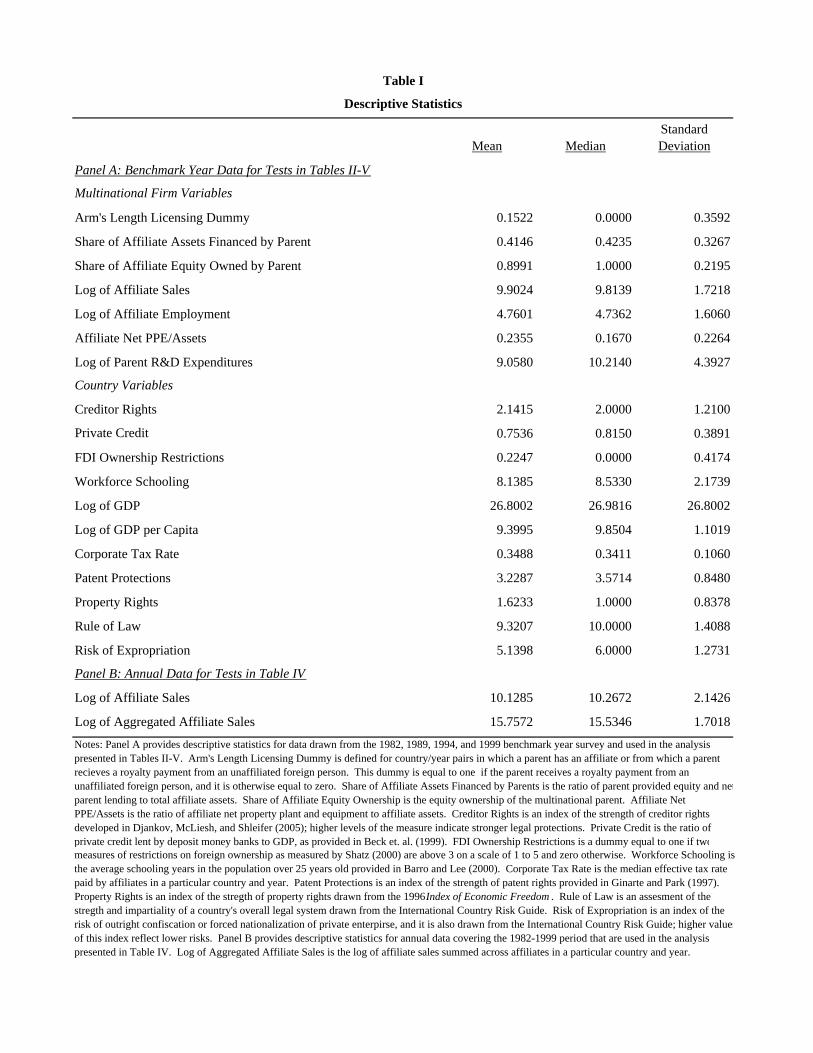
Mean MedianStandard Deviation

Panel A: Benchmark Year Data for Tests in Tables II-V

Multinational Firm Variables

Arm's Length Licensing Dummy 0.1522 0.0000 0.3592

Share of Affiliate Assets Financed by Parent 0.4146 0.4235 0.3267

Share of Affiliate Equity Owned by Parent 0.8991 1.0000 0.2195

Log of Affiliate Sales 9.9024 9.8139 1.7218

Log of Affiliate Employment 4.7601 4.7362 1.6060

Affiliate Net PPE/Assets 0.2355 0.1670 0.2264

Log of Parent R&D Expenditures 9.0580 10.2140 4.3927

Country Variables

Creditor Rights 2.1415 2.0000 1.2100

Private Credit 0.7536 0.8150 0.3891

FDI Ownership Restrictions 0.2247 0.0000 0.4174

Workforce Schooling 8.1385 8.5330 2.1739

Log of GDP 26.8002 26.9816 26.8002

Log of GDP per Capita 9.3995 9.8504 1.1019

Corporate Tax Rate 0.3488 0.3411 0.1060

Patent Protections 3.2287 3.5714 0.8480

Property Rights 1.6233 1.0000 0.8378

Rule of Law 9.3207 10.0000 1.4088

Risk of Expropriation 5.1398 6.0000 1.2731

Panel B: Annual Data for Tests in Table IV

Log of Affiliate Sales 10.1285 10.2672 2.1426

Log of Aggregated Affiliate Sales 15.7572 15.5346 1.7018

Table I

Descriptive Statistics

Notes: Panel A provides descriptive statistics for data drawn from the 1982, 1989, 1994, and 1999 benchmark year survey and used in the analysis presented in Tables II-V. Arm's Length Licensing Dummy is defined for country/year pairs in which a parent has an affiliate or from which a parent recieves a royalty payment from an unaffiliated foreign person. This dummy is equal to one if the parent receives a royalty payment from an unaffiliated foreign person, and it is otherwise equal to zero. Share of Affiliate Assets Financed by Parents is the ratio of parent provided equity and netparent lending to total affiliate assets. Share of Affiliate Equity Ownership is the equity ownership of the multinational parent. Affiliate Net PPE/Assets is the ratio of affiliate net property plant and equipment to affiliate assets. Creditor Rights is an index of the strength of creditor rights developed in Djankov, McLiesh, and Shleifer (2005); higher levels of the measure indicate stronger legal protections. Private Credit is the ratio of private credit lent by deposit money banks to GDP, as provided in Beck et. al. (1999). FDI Ownership Restrictions is a dummy equal to one if twomeasures of restrictions on foreign ownership as measured by Shatz (2000) are above 3 on a scale of 1 to 5 and zero otherwise. Workforce Schooling is the average schooling years in the population over 25 years old provided in Barro and Lee (2000). Corporate Tax Rate is the median effective tax rate paid by affiliates in a particular country and year. Patent Protections is an index of the strength of patent rights provided in Ginarte and Park (1997). Property Rights is an index of the stregth of property rights drawn from the 1996 Index of Economic Freedom . Rule of Law is an assesment of the stregth and impartiality of a country's overall legal system drawn from the International Country Risk Guide. Risk of Expropriation is an index of the risk of outright confiscation or forced nationalization of private enterpirse, and it is also drawn from the International Country Risk Guide; higher valuesof this index reflect lower risks. Panel B provides descriptive statistics for annual data covering the 1982-1999 period that are used in the analysis presented in Table IV. Log of Aggregated Affiliate Sales is the log of affiliate sales summed across affiliates in a particular country and year.

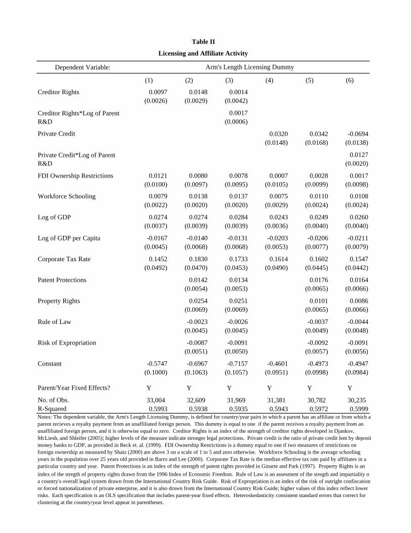
Dependent Variable:

(1) (2) (3) (4) (5) (6)

Creditor Rights 0.0097 0.0148 0.0014(0.0026) (0.0029) (0.0042)

0.0017(0.0006)

Private Credit 0.0320 0.0342 -0.0694(0.0148) (0.0168) (0.0138)

0.0127(0.0020)

FDI Ownership Restrictions 0.0121 0.0080 0.0078 0.0007 0.0028 0.0017(0.0100) (0.0097) (0.0095) (0.0105) (0.0099) (0.0098)

Workforce Schooling 0.0079 0.0138 0.0137 0.0075 0.0110 0.0108(0.0022) (0.0020) (0.0020) (0.0029) (0.0024) (0.0024)

Log of GDP 0.0274 0.0274 0.0284 0.0243 0.0249 0.0260(0.0037) (0.0039) (0.0039) (0.0036) (0.0040) (0.0040)

Log of GDP per Capita -0.0167 -0.0140 -0.0131 -0.0203 -0.0206 -0.0211(0.0045) (0.0068) (0.0068) (0.0053) (0.0077) (0.0079)

0.1452 0.1830 0.1733 0.1614 0.1602 0.1547(0.0492) (0.0470) (0.0453) (0.0490) (0.0445) (0.0442)

Patent Protections 0.0142 0.0134 0.0176 0.0164(0.0054) (0.0053) (0.0065) (0.0066)

Property Rights 0.0254 0.0251 0.0101 0.0086(0.0069) (0.0069) (0.0065) (0.0066)

Rule of Law -0.0023 -0.0026 -0.0037 -0.0044(0.0045) (0.0045) (0.0049) (0.0048)

Risk of Expropriation -0.0087 -0.0091 -0.0092 -0.0091(0.0051) (0.0050) (0.0057) (0.0056)

Constant -0.5747 -0.6967 -0.7157 -0.4601 -0.4973 -0.4947(0.1000) (0.1063) (0.1057) (0.0951) (0.0998) (0.0984)

Parent/Year Fixed Effects? Y Y Y Y Y Y

No. of Obs. 33,004 32,609 31,969 31,381 30,782 30,235 R-Squared 0.5993 0.5938 0.5935 0.5943 0.5972 0.5999

Private Credit*Log of Parent R&D

Corporate Tax Rate

Notes: The dependent variable, the Arm's Length Licensing Dummy, is defined for country/year pairs in which a parent has an affiliate or from which a parent recieves a royalty payment from an unaffiliated foreign person. This dummy is equal to one if the parent receives a royalty payment from an unaffiliated foreign person, and it is otherwise equal to zero. Creditor Rights is an index of the strength of creditor rights developed in Djankov, McLiesh, and Shleifer (2005); higher levels of the measure indicate stronger legal protections. Private credit is the ratio of private credit lent by deposit money banks to GDP, as provided in Beck et. al. (1999). FDI Ownership Restrictions is a dummy equal to one if two measures of restrictions on foreign ownership as measured by Shatz (2000) are above 3 on a scale of 1 to 5 and zero otherwise. Workforce Schooling is the average schooling years in the population over 25 years old provided in Barro and Lee (2000). Corporate Tax Rate is the median effective tax rate paid by affiliates in a particular country and year. Patent Protections is an index of the strength of patent rights provided in Ginarte and Park (1997). Property Rights is an index of the stregth of property rights drawn from the 1996 Index of Economic Freedom. Rule of Law is an assesment of the stregth and impartiality ofa country's overall legal system drawn from the International Country Risk Guide. Risk of Expropriation is an index of the risk of outright confiscation or forced nationalization of private enterpirse, and it is also drawn from the International Country Risk Guide; higher values of this index reflect lower risks. Each specification is an OLS specification that includes parent-year fixed effects. Heteroskedasticity consistent standard errors that correct for clustering at the country/year level appear in parentheses.

Table II

Licensing and Affiliate Activity

Arm's Length Licensing Dummy

Creditor Rights*Log of Parent R&D

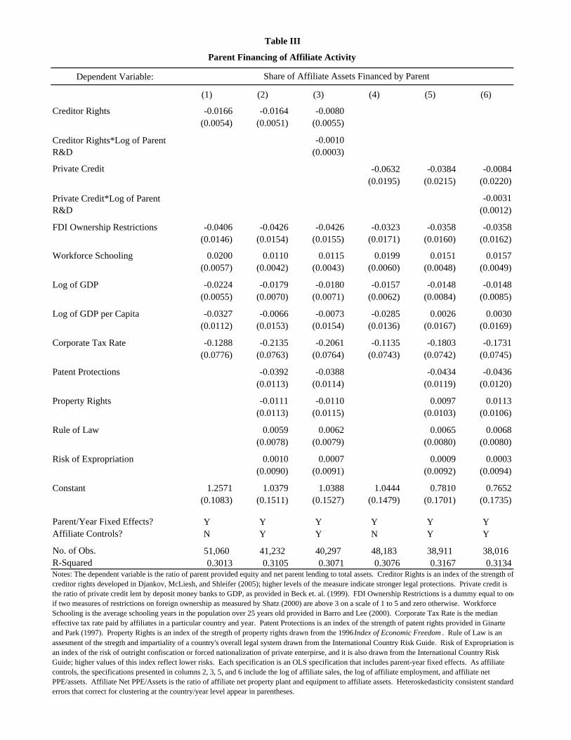
Dependent Variable:

(1) (2) (3) (4) (5) (6)

Creditor Rights -0.0166 -0.0164 -0.0080(0.0054) (0.0051) (0.0055)

-0.0010(0.0003)

Private Credit -0.0632 -0.0384 -0.0084(0.0195) (0.0215) (0.0220)

-0.0031(0.0012)

FDI Ownership Restrictions -0.0406 -0.0426 -0.0426 -0.0323 -0.0358 -0.0358(0.0146) (0.0154) (0.0155) (0.0171) (0.0160) (0.0162)

Workforce Schooling 0.0200 0.0110 0.0115 0.0199 0.0151 0.0157(0.0057) (0.0042) (0.0043) (0.0060) (0.0048) (0.0049)

Log of GDP -0.0224 -0.0179 -0.0180 -0.0157 -0.0148 -0.0148(0.0055) (0.0070) (0.0071) (0.0062) (0.0084) (0.0085)

Log of GDP per Capita -0.0327 -0.0066 -0.0073 -0.0285 0.0026 0.0030(0.0112) (0.0153) (0.0154) (0.0136) (0.0167) (0.0169)

-0.1288 -0.2135 -0.2061 -0.1135 -0.1803 -0.1731(0.0776) (0.0763) (0.0764) (0.0743) (0.0742) (0.0745)

Patent Protections -0.0392 -0.0388 -0.0434 -0.0436(0.0113) (0.0114) (0.0119) (0.0120)

Property Rights -0.0111 -0.0110 0.0097 0.0113(0.0113) (0.0115) (0.0103) (0.0106)

Rule of Law 0.0059 0.0062 0.0065 0.0068(0.0078) (0.0079) (0.0080) (0.0080)

Risk of Expropriation 0.0010 0.0007 0.0009 0.0003(0.0090) (0.0091) (0.0092) (0.0094)

Constant 1.2571 1.0379 1.0388 1.0444 0.7810 0.7652(0.1083) (0.1511) (0.1527) (0.1479) (0.1701) (0.1735)

Parent/Year Fixed Effects? Y Y Y Y Y YAffiliate Controls? N Y Y N Y Y

No. of Obs. 51,060 41,232 40,297 48,183 38,911 38,016 R-Squared 0.3013 0.3105 0.3071 0.3076 0.3167 0.3134

assesment of the stregth and impartiality of a country's overall legal system drawn from the International Country Risk Guide. Risk of Expropriation is an index of the risk of outright confiscation or forced nationalization of private enterpirse, and it is also drawn from the International Country Risk Guide; higher values of this index reflect lower risks. Each specification is an OLS specification that includes parent-year fixed effects. As affiliate controls, the specifications presented in columns 2, 3, 5, and 6 include the log of affiliate sales, the log of affiliate employment, and affiliate net PPE/assets. Affiliate Net PPE/Assets is the ratio of affiliate net property plant and equipment to affiliate assets. Heteroskedasticity consistent standard errors that correct for clustering at the country/year level appear in parentheses.

Notes: The dependent variable is the ratio of parent provided equity and net parent lending to total assets. Creditor Rights is an index of the strength of creditor rights developed in Djankov, McLiesh, and Shleifer (2005); higher levels of the measure indicate stronger legal protections. Private credit is the ratio of private credit lent by deposit money banks to GDP, as provided in Beck et. al. (1999). FDI Ownership Restrictions is a dummy equal to oneif two measures of restrictions on foreign ownership as measured by Shatz (2000) are above 3 on a scale of 1 to 5 and zero otherwise. Workforce Schooling is the average schooling years in the population over 25 years old provided in Barro and Lee (2000). Corporate Tax Rate is the median effective tax rate paid by affiliates in a particular country and year. Patent Protections is an index of the strength of patent rights provided in Ginarte and Park (1997). Property Rights is an index of the stregth of property rights drawn from the 1996 Index of Economic Freedom . Rule of Law is an

Table III

Parent Financing of Affiliate Activity

Share of Affiliate Assets Financed by Parent

Corporate Tax Rate

Creditor Rights*Log of Parent R&D

Private Credit*Log of Parent R&D

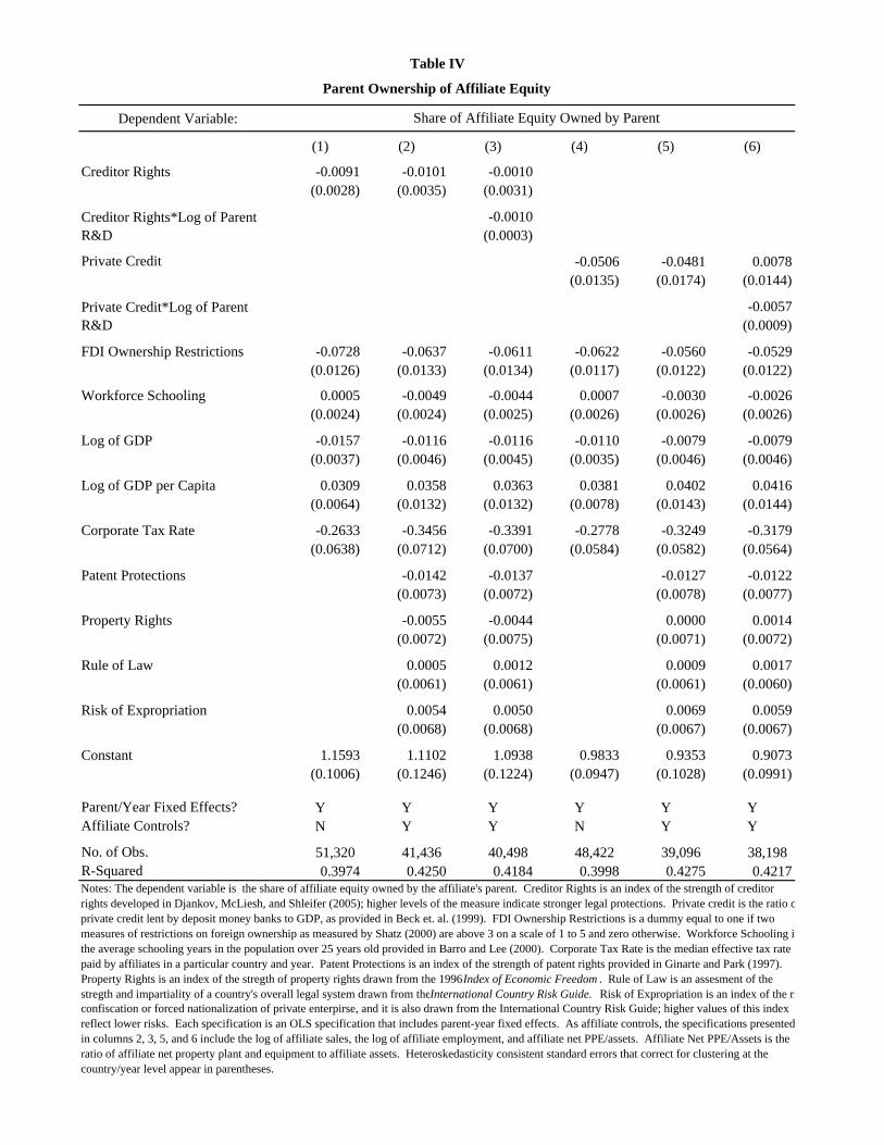
Dependent Variable:

(1) (2) (3) (4) (5) (6)

Creditor Rights -0.0091 -0.0101 -0.0010(0.0028) (0.0035) (0.0031)

-0.0010(0.0003)

Private Credit -0.0506 -0.0481 0.0078(0.0135) (0.0174) (0.0144)

-0.0057(0.0009)

FDI Ownership Restrictions -0.0728 -0.0637 -0.0611 -0.0622 -0.0560 -0.0529(0.0126) (0.0133) (0.0134) (0.0117) (0.0122) (0.0122)

Workforce Schooling 0.0005 -0.0049 -0.0044 0.0007 -0.0030 -0.0026(0.0024) (0.0024) (0.0025) (0.0026) (0.0026) (0.0026)

Log of GDP -0.0157 -0.0116 -0.0116 -0.0110 -0.0079 -0.0079(0.0037) (0.0046) (0.0045) (0.0035) (0.0046) (0.0046)

Log of GDP per Capita 0.0309 0.0358 0.0363 0.0381 0.0402 0.0416(0.0064) (0.0132) (0.0132) (0.0078) (0.0143) (0.0144)

-0.2633 -0.3456 -0.3391 -0.2778 -0.3249 -0.3179(0.0638) (0.0712) (0.0700) (0.0584) (0.0582) (0.0564)

Patent Protections -0.0142 -0.0137 -0.0127 -0.0122(0.0073) (0.0072) (0.0078) (0.0077)

Property Rights -0.0055 -0.0044 0.0000 0.0014(0.0072) (0.0075) (0.0071) (0.0072)

Rule of Law 0.0005 0.0012 0.0009 0.0017(0.0061) (0.0061) (0.0061) (0.0060)

Risk of Expropriation 0.0054 0.0050 0.0069 0.0059(0.0068) (0.0068) (0.0067) (0.0067)

Constant 1.1593 1.1102 1.0938 0.9833 0.9353 0.9073(0.1006) (0.1246) (0.1224) (0.0947) (0.1028) (0.0991)

Parent/Year Fixed Effects? Y Y Y Y Y YAffiliate Controls? N Y Y N Y Y

No. of Obs. 51,320 41,436 40,498 48,422 39,096 38,198 R-Squared 0.3974 0.4250 0.4184 0.3998 0.4275 0.4217

Private Credit*Log of Parent R&D

Corporate Tax Rate

Notes: The dependent variable is the share of affiliate equity owned by the affiliate's parent. Creditor Rights is an index of the strength of creditor rights developed in Djankov, McLiesh, and Shleifer (2005); higher levels of the measure indicate stronger legal protections. Private credit is the ratio oprivate credit lent by deposit money banks to GDP, as provided in Beck et. al. (1999). FDI Ownership Restrictions is a dummy equal to one if two measures of restrictions on foreign ownership as measured by Shatz (2000) are above 3 on a scale of 1 to 5 and zero otherwise. Workforce Schooling ithe average schooling years in the population over 25 years old provided in Barro and Lee (2000). Corporate Tax Rate is the median effective tax rate paid by affiliates in a particular country and year. Patent Protections is an index of the strength of patent rights provided in Ginarte and Park (1997). Property Rights is an index of the stregth of property rights drawn from the 1996 Index of Economic Freedom . Rule of Law is an assesment of the stregth and impartiality of a country's overall legal system drawn from theInternational Country Risk Guide. Risk of Expropriation is an index of the riconfiscation or forced nationalization of private enterpirse, and it is also drawn from the International Country Risk Guide; higher values of this index reflect lower risks. Each specification is an OLS specification that includes parent-year fixed effects. As affiliate controls, the specifications presented in columns 2, 3, 5, and 6 include the log of affiliate sales, the log of affiliate employment, and affiliate net PPE/assets. Affiliate Net PPE/Assets is the ratio of affiliate net property plant and equipment to affiliate assets. Heteroskedasticity consistent standard errors that correct for clustering at the country/year level appear in parentheses.

Table IV

Parent Ownership of Affiliate Equity

Share of Affiliate Equity Owned by Parent

Creditor Rights*Log of Parent R&D

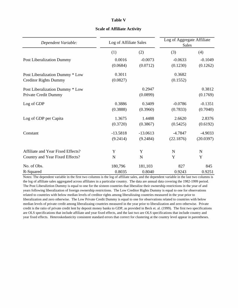
Dependent Variable:

(1) (2) (3) (4)

Post Liberalization Dummy 0.0016 -0.0073 -0.0633 -0.1049(0.0684) (0.0712) (0.1230) (0.1262)

0.3011 0.3682(0.0827) (0.1552)

0.2947 0.3812(0.0899) (0.1769)

Log of GDP 0.3886 0.3409 -0.0786 -0.1351(0.3888) (0.3960) (0.7833) (0.7040)

Log of GDP per Capita 1.3675 1.4488 2.6620 2.8376(0.3720) (0.3867) (0.5425) (0.6192)

Constant -13.5818 -13.0613 -4.7847 -4.9033(9.2414) (9.2484) (22.1876) (20.0397)

Affiliate and Year Fixed Effects? Y Y N NCountry and Year Fixed Effects? N N Y Y

No. of Obs. 180,796 181,103 827 845 R-Squared 0.8035 0.8040 0.9243 0.9251

Table V

Scale of Affiliate Activity

year fixed effects. Heteroskedasticity consistent standard errors that correct for clustering at the country level appear in parentheses.

Log of Affiliate Sales Log of Aggregate Affiliate Sales

Notes: The dependent variable in the first two columns is the log of affiliate sales, and the dependent variable in the last two columns is the log of affiliate sales aggregated across affiliates in a particular country. The data are annual data covering the 1982-1999 period. The Post Liberaliztion Dummy is equal to one for the sixteen countries that liberalize their ownership restrictions in the year of and years following liberalization of foreign ownership restrictions. The Low Creditor Rights Dummy is equal to one for observations related to countries with below median levels of creditor rights among liberalizaing countries measured in the year prior to liberalization and zero otherwise. The Low Private Credit Dummy is equal to one for observations related to countries with below median levels of private credit among liberalizaing countries measured in the year prior to liberalization and zero otherwise. Private credit is the ratio of private credit lent by deposit money banks to GDP, as provided in Beck et. al. (1999). The first two specifications are OLS specifications that include affiliate and year fixed effects, and the last two are OLS specifications that include country and

Post Liberalization Dummy * Low Creditor Rights Dummy

Post Liberalization Dummy * Low Private Credit Dummy

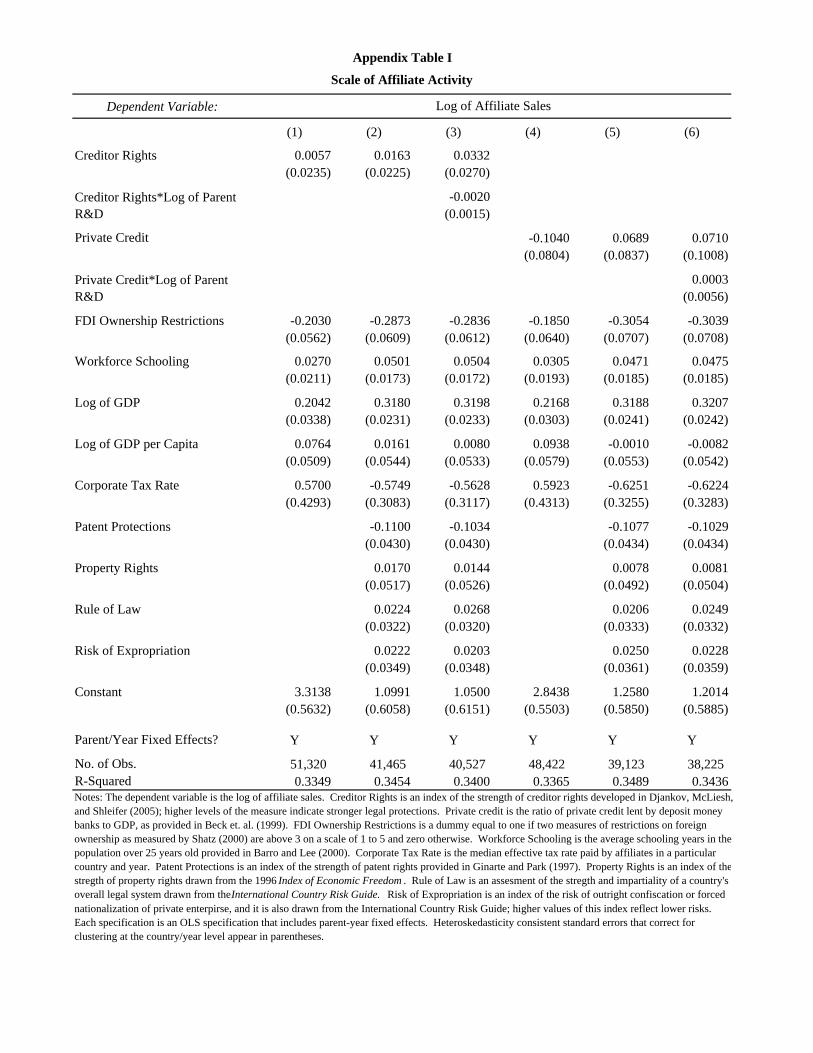
Dependent Variable:

(1) (2) (3) (4) (5) (6)

Creditor Rights 0.0057 0.0163 0.0332(0.0235) (0.0225) (0.0270)

-0.0020(0.0015)

Private Credit -0.1040 0.0689 0.0710(0.0804) (0.0837) (0.1008)

0.0003(0.0056)

FDI Ownership Restrictions -0.2030 -0.2873 -0.2836 -0.1850 -0.3054 -0.3039(0.0562) (0.0609) (0.0612) (0.0640) (0.0707) (0.0708)

Workforce Schooling 0.0270 0.0501 0.0504 0.0305 0.0471 0.0475(0.0211) (0.0173) (0.0172) (0.0193) (0.0185) (0.0185)

Log of GDP 0.2042 0.3180 0.3198 0.2168 0.3188 0.3207(0.0338) (0.0231) (0.0233) (0.0303) (0.0241) (0.0242)

Log of GDP per Capita 0.0764 0.0161 0.0080 0.0938 -0.0010 -0.0082(0.0509) (0.0544) (0.0533) (0.0579) (0.0553) (0.0542)

0.5700 -0.5749 -0.5628 0.5923 -0.6251 -0.6224(0.4293) (0.3083) (0.3117) (0.4313) (0.3255) (0.3283)

Patent Protections -0.1100 -0.1034 -0.1077 -0.1029(0.0430) (0.0430) (0.0434) (0.0434)

Property Rights 0.0170 0.0144 0.0078 0.0081(0.0517) (0.0526) (0.0492) (0.0504)

Rule of Law 0.0224 0.0268 0.0206 0.0249(0.0322) (0.0320) (0.0333) (0.0332)

Risk of Expropriation 0.0222 0.0203 0.0250 0.0228(0.0349) (0.0348) (0.0361) (0.0359)

Constant 3.3138 1.0991 1.0500 2.8438 1.2580 1.2014(0.5632) (0.6058) (0.6151) (0.5503) (0.5850) (0.5885)

Parent/Year Fixed Effects? Y Y Y Y Y Y

No. of Obs. 51,320 41,465 40,527 48,422 39,123 38,225 R-Squared 0.3349 0.3454 0.3400 0.3365 0.3489 0.3436

nationalization of private enterpirse, and it is also drawn from the International Country Risk Guide; higher values of this index reflect lower risks. Each specification is an OLS specification that includes parent-year fixed effects. Heteroskedasticity consistent standard errors that correct for clustering at the country/year level appear in parentheses.

Notes: The dependent variable is the log of affiliate sales. Creditor Rights is an index of the strength of creditor rights developed in Djankov, McLiesh, and Shleifer (2005); higher levels of the measure indicate stronger legal protections. Private credit is the ratio of private credit lent by deposit money banks to GDP, as provided in Beck et. al. (1999). FDI Ownership Restrictions is a dummy equal to one if two measures of restrictions on foreign ownership as measured by Shatz (2000) are above 3 on a scale of 1 to 5 and zero otherwise. Workforce Schooling is the average schooling years in the population over 25 years old provided in Barro and Lee (2000). Corporate Tax Rate is the median effective tax rate paid by affiliates in a particular country and year. Patent Protections is an index of the strength of patent rights provided in Ginarte and Park (1997). Property Rights is an index of thestregth of property rights drawn from the 1996 Index of Economic Freedom . Rule of Law is an assesment of the stregth and impartiality of a country's overall legal system drawn from the International Country Risk Guide. Risk of Expropriation is an index of the risk of outright confiscation or forced

Appendix Table I

Creditor Rights*Log of Parent R&D

Private Credit*Log of Parent R&D

Corporate Tax Rate

Scale of Affiliate Activity

Log of Affiliate Sales