Multimedia Traffic EngineeringThe Bursty Data Model

John T. Chapman

Distinguished Engineer

Cisco Systems

jchapman@cisco.com

Opening Comments

A) 250 per upstream

B) One less than the number it takes to bring down the whole plant

C) No clue

D) It depends

• Multiple choice question:– How many cable modems will a

CMTS support?

• This presentation will focus on a model for DOCSIS bandwidth

The Basic Concept

• The answer is:

• The CMTS bandwidth is predictable.– But there does not exist a good model for the

CM bandwidth required.– As such, the question goes unanswered.

CMTS Bandwidth Available

CM Bandwidth Required= Number of CMs Supported

IP Data “Discounts”

• Bandwidth “discounts” for data:– Example: 1 dn, 6 up, 2000 HHP per upstream

Upstream Bandwidth 2.5 Mbps / 2000 HHP => 1.25 kbps per HHP@ 10% Market Penetration => 12 kbps per Subscriber @ 20% logged on => 60 kbps Avg per User @ 20% downloading => 300 kbps per User

Bandwidth Ratio 550 kbps Downstream/ 300 kbps Upstream => 1.8 Dn/Up BW

Downstream Bandwidth 26 Mbps / 6 Rx / 2000 HHP => 2.2 kbps per HHP @ 10 % Market Penetration => 20 kbps per Subscriber @ 20 % logged on => 100 kbps avg per User @ 20% downloading => 500 kbps peak per User

250x

Bursty Data Model Requirements

• Simplicity:– Equations must fit on the back of an envelope.– Easy to put into a spreadsheet.– Easy to use by all. Approximations are fine. Complication

avoided.• Usefulness:

– Must relate to measured parameters– Must be usable for bandwidth calculations

• VoIP and broadcast quality video handled with separate models

The Role of the Model

• Modeling what already exists is interesting, but modeling what does not yet exist is what is most important

TheModel

MeasuredResults

PredictedResults

GrowthProjections

Theory

current

future

Model Scenarios

• This model is derived in part from a behavioral description of what the subscriber and operator see when looking at the network.

• Defining 1 second and 5 minute measurement intervals provides two operating points for the network.

time

time

time

bit rate

bit rate

bit rate

packets

1 secondenvelope

5 minuteenvelope

“average scenario”

“peak scenario”

“max scenario”

The Three Model Scenarios

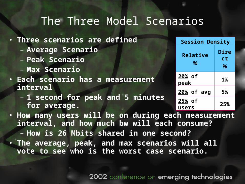
• Three scenarios are defined– Average Scenario– Peak Scenario– Max Scenario

• Each scenario has a measurement interval– 1 second for peak and 5 minutes

for average.• How many users will be on during each measurement

interval, and how much bw will each consume? – How is 26 Mbits shared in one second?

• The average, peak, and max scenarios will all vote to see who is the worst case scenario.

Session Density

Relative

%

Direct

%

20% of peak 1%

20% of avg 5%

25% of users 25%

Wall Street Analogy

• Wall Street Analogy• Avg rate == quarterly sales• Peak rate == weekly sales• Packet rate == daily sales

• Quarterly sales can be predicted reasonable well. Weekly sales have large variations, whereas daily sales can be anything. Yet, a good factory must be able to respond well to daily and weekly fluctuations to be efficient.

User Data Profile

• Bandwidth numbers are the most important• Packet size and rate is tracked so that overhead per

packet can be calculated and impact on system switching can be assessed.

Down

Stream

Data

Bit Rate

kbps

Max 2,000

Peak 256

Average 80

Up

Stream

Data

Bit Rate

kbps

Max 384

Peak 100

Average 24

Profile

Pkt Size

bytes

Pkt Rate

pps

1518 165

1518 21

400 25

Profile

Pkt Size

bytes

Pkt Rate

pps

1518 32

1518 8

64 47

Using Measured Results

• Monitoring of IP packets for both measurement intervals can supply– Mix of applications by examining the TCP/UDP port number– Number of users by looking for unique IP addresses – Size of packet per application

• The following can be calculated for each scenario:– Bandwidth per user.– Nominal packet size per user– Nominal PPS per user.

• These measurements provide the basics for the Bursty Data Model.

Generation of Subscriber Profile

Sum of {Application profiles * market penetration}

=> Web Traffic * %MPa

+ E-mail * %MPa

+ Gaming * %MPa

+ Video Streaming * %MPa

+ Audio Streaming * %MPa

+ etc

MPa = market penetrationof application within

subscriber base

Down

Stream

Data

Bit Rate

kbps

Max 2,000

Peak 256

Average 80

Up

Stream

Data

Bit Rate

kbps

Max 384

Peak 100

Average 24

Profile

Pkt Size

bytes

Pkt Rate

pps

1518 165

1518 21

400 25

Profile

Pkt Size

bytes

Pkt Rate

pps

1518 32

1518 8

64 47

Down

StreamBit

RatePkt Size

Peak 256 1518

Average 80 400

Up

StreamBit

RatePkt Size

Peak 100 1518

Average 24 400

Down

StreamBit

RatePkt Size

Peak 256 1518

Average 80 400

Up

StreamBit

RatePkt Size

Peak 100 1518

Average 24 400

Multiple Tiers of Service

Sum of {tier profiles * market penetration}

=> Platinum * %MPt

+ Gold * %MPt

+ Silver * %MPt

MPt = market penetrationof service level within

subscriber base

Platinum

Gold

Silver

Down

Stream

Data

Bit Rate

kbps

Max 2,000

Peak 256

Average 80

Up

Stream

Data

Bit Rate

kbps

Max 384

Peak 100

Average 24

Profile

Pkt Size

bytes

Pkt Rate

pps

1518 165

1518 21

400 25

Profile

Pkt Size

bytes

Pkt Rate

pps

1518 32

1518 8

64 47

Down

StreamBit

RatePkt Size

Max 2000 1518

Peak 256 1518

Average 80 400

Up

StreamBit

RatePkt Size

Max 384 1518

Peak 100 1518

Average 24 400

Down

StreamBit

RatePkt Size

Max 2000 1518

Peak 256 1518

Average 80 400

Up

StreamBit

RatePkt Size

Max 384 1518

Peak 100 1518

Average 24 400

Down

StreamBit

RatePkt Size

Max 2000 1518

Peak 256 1518

Average 80 400

Up

StreamBit

RatePkt Size

Max 384 1518

Peak 100 1518

Average 24 400

Downstream Calculation

• Inputs to the model are underlined• The inverse of MP% for avg, peak, and max equals the

over-subscription for each scenario.

Down

Stream

Data Profile

Bit Rate

kbps

Pkt Size

bytes

Pkt Rate

pps

Max 2000 1518 165

Peak 256 1518 21

Average 80 400 25

Max Users per Downstream: 1150

Users per Down

stream

1173

1832

1150

Downstream

Pkt Rate

pps

Ses-sions

1931 12

1931 92

7185 287

D/S Payload 26.25 Mbps

D/S Admission 90%

Session Density

Relative

%

Direct

%

20% of peak 1%

20% of avg 5%

25% of users 25%

Upstream Calculation

• Average BW is the limiting case

Up

Stream

Data Profile

Bit Rate

kbps

Pkt Size

bytes

Pkt Rate

pps

Max 384 1518 32

Peak 100 1518 8

Average 24 64 47

Max Users per Upstream: 207

Upstream

Ses-sions

Pkt Rate

pps

5 150

18 150

52 2424

Users per Upstream

475

365

207

U/S Payload 2.56 Mbps

U/S Admission 80%

Usage

Relative

%

Direct

%

20% of peak 1%

20% of avg 5%

25% of users 25%

Downstream & Upstream

• In this example, the system is downstream limited

DirectionSubs

allowedLC

ratio

Subs per groupSubs per

Group

Max HHP per

Directionmax final

Downstream 1150 1 11501150

766 7664

Upstream 207 6 1241 128 1277Users per HHP 1.5

%MP of data 10%

Bursty Data Model Fundamentals

– Calculation can be done backwards, starting with the number of subscribers and ending with the bandwidth profile.

MediaProfile

SessionDensity

Users

UserProfile

=

Traffic Barometer

• Using “% logged on” and “% downloading” may not be easily measurable. What is measurable from the CMTS is:– CMs per upstream & downstream– Bandwidth in terms of Mbps and PPS per u/s, d/s, and

WAN port.• Use CMTS statistics to calculate (for down and up)

– Average Mbps per CM: for example, 20 kbps– Average PPS per CM: for example, 5 PPS– Average packet size: for example, 400 bytes

The Complete Profile

• A more complete subscriber profile should include – Bandwidth– Latency– Jitter– Allowable packet loss

• Last three requirements are more QOS related• Service levels (Silver, Gold, Platinum) could differ based upon

bandwidth only, QOS only, or both bandwidth and QOS.– A low latency service for gaming, for example, would be

interesting.

Closing Comments

• Networks which carry data, voice, and video must be engineered if they are to operate properly.

• There is room for other models. However they should– parameters determined through intuition, calculation,

and/or measurement– relates to all traffic types and service tiers– can be used to calculate the network loading

• The MMTE Bursty Data Model solves the equation:

CMTS Bandwidth Available

CM Bandwidth Required= Number of CMs Supported