
Multilevel Monte Carlo for exponential Lévy models · multilevel Monte Carlo method applied to...
32
Finance Stoch (2017) 21:995–1026 DOI 10.1007/s00780-017-0341-7 Multilevel Monte Carlo for exponential Lévy models Michael B. Giles 1 · Yuan Xia 1 Received: 20 March 2014 / Accepted: 9 May 2017 / Published online: 6 September 2017 © The Author(s) 2017. This article is published with open access at Springerlink.com Abstract We apply the multilevel Monte Carlo method for option pricing problems using exponential Lévy models with a uniform timestep discretisation. For look- back and barrier options, we derive estimates of the convergence rate of the error introduced by the discrete monitoring of the running supremum of a broad class of Lévy processes. We then use these to obtain upper bounds on the multilevel Monte Carlo variance convergence rate for the variance gamma, NIG and α-stable processes. We also provide an analysis of a trapezoidal approximation for Asian options. Our method is illustrated by numerical experiments. Keywords Multilevel Monte Carlo · Exponential Lévy models · Asian options · Lookback options · Barrier options Mathematics Subject Classification (2010) 65C05 · 91G60 JEL Classification C15 · C63 1 Introduction Exponential Lévy models are based on the assumption that asset returns follow a Lévy process [25, 10]. The asset price follows S t = S 0 exp(X t ) B Y. Xia [email protected] M.B. Giles [email protected] 1 Mathematical Institute, Oxford University, Oxford, UK
Transcript of Multilevel Monte Carlo for exponential Lévy models · multilevel Monte Carlo method applied to...
Finance Stoch (2017) 21:995–1026DOI 10.1007/s00780-017-0341-7
Multilevel Monte Carlo for exponential Lévy models
Michael B. Giles1 · Yuan Xia1
Received: 20 March 2014 / Accepted: 9 May 2017 / Published online: 6 September 2017© The Author(s) 2017. This article is published with open access at Springerlink.com
Abstract We apply the multilevel Monte Carlo method for option pricing problemsusing exponential Lévy models with a uniform timestep discretisation. For look-back and barrier options, we derive estimates of the convergence rate of the errorintroduced by the discrete monitoring of the running supremum of a broad class ofLévy processes. We then use these to obtain upper bounds on the multilevel MonteCarlo variance convergence rate for the variance gamma, NIG and α-stable processes.We also provide an analysis of a trapezoidal approximation for Asian options. Ourmethod is illustrated by numerical experiments.
Keywords Multilevel Monte Carlo · Exponential Lévy models · Asian options ·Lookback options · Barrier options
Mathematics Subject Classification (2010) 65C05 · 91G60
JEL Classification C15 · C63
1 Introduction
Exponential Lévy models are based on the assumption that asset returns follow aLévy process [25, 10]. The asset price follows
St = S0 exp(Xt )
B Y. [email protected]
M.B. [email protected]
1 Mathematical Institute, Oxford University, Oxford, UK
996 M.B. Giles, Y. Xia
where X is an (m,σ, ν)-Lévy process, i.e.,
Xt = mt + σBt +∫ t
0
∫{|z|≥1}
z J (dz,ds) +∫ t
0
∫{|z|<1}
z(J (dz,ds) − ν(dz)ds
),
where m is a constant, B is a Brownian motion, J is the jump measure and ν is theLévy measure (cf. [24, Theorem I.42]).
Models with jumps give an intuitive explanation of implied volatility skews andsmiles in the index option market and foreign exchange market ([10, Chap. 11]). Thejump fear is mainly on the downside in the equity market which produces a premiumfor low-strike options; the jump risk is symmetric in the foreign exchange market sothat the implied volatility has a smile shape. Chapter 7 in [10] shows that modelsbuilding on pure jump processes can reproduce the stylised facts of asset returns, likeheavy tails and the asymmetric distribution of increments. Since pure jump processesof finite activity without a diffusion component cannot generate a realistic path, it isnatural to allow the jump activity to be infinite. In this work, we deal with infinite-activity pure jump exponential Lévy models, in particular models driven by variancegamma (VG), normal inverse Gaussian (NIG) and α-stable processes which allowdirect simulation of increments.
We are interested in estimating the expected payoff value E[f (S)] in option pric-ing problems. In the case of European options, it is possible to directly sample the fi-nal value of the underlying Lévy process, but for Asian, lookback and barrier options,the option value depends on functionals of the Lévy process and so it is necessary toapproximate those. In the case of a VG model with a lookback option, the conver-gence results in [13] show that to achieve an O(ε) root mean square (RMS) errorusing a standard Monte Carlo method with a uniform timestep discretisation requiresO(ε−2) paths, each with O(ε−1) timesteps, leading to a computational complexityof O(ε−3).
In the case of a simple Brownian diffusion, Giles [16, 17] introduced a multilevelMonte Carlo (MLMC) method, reducing the computational complexity from O(ε−3)
to O(ε−2) for a variety of payoffs. The objective of this paper is to investigate whethersimilar benefits can be obtained for exponential Lévy processes.
Various researchers have investigated simulation methods for the running maxi-mum of Lévy processes. Reference [15] develops an adaptive Monte Carlo methodfor functionals of killed Lévy processes with a controlled bias. Small-time asymp-totic expansions of the exit probability are given with computable error bounds. Forevaluating the exit probability when the barrier is close to the starting point of theprocess, this algorithm outperforms a uniform discretisation significantly. Reference[21] develops a novel Wiener–Hopf Monte Carlo method to generate the joint distri-bution of (XT , sup0≤t≤T Xt ) which is further extended to MLMC in [14], obtainingan RMS error ε with a computational complexity of O(ε−3) for Lévy processes withbounded variation, and O
(ε−4
)for processes with infinite variation. The method
currently cannot be directly applied to VG, NIG and α-stable processes. References[12, 11] adapt MLMC to Lévy-driven SDEs with payoffs which are Lipschitz withrespect to the supremum norm. If the Lévy process does not incorporate a Brownianprocess, reference [11] obtains an O(ε−(6β)/(4−β)) upper bound on the worst casecomputational complexity, where β is the BG index which will be defined later.
Multilevel Monte Carlo for exponential Lévy models 997
In contrast to those advanced techniques, we take the discretely monitored maxi-mum based on a uniform timestep discretisation of the Lévy process as the approxi-mation. The outline of the work is as follows. First we review the multilevel MonteCarlo method and present the three Lévy processes we consider in our numericalexperiments. To prepare for the analysis of the multilevel variance of lookback andbarrier, we bound the convergence rate of the discretely monitored running maximumfor a large class of Lévy processes whose Lévy measures have a power law behaviourfor small jumps, and have exponential tails. Based on this, we conclude by boundingthe variance of the multilevel estimators. Numerical results are then presented for themultilevel Monte Carlo method applied to Asian, lookback and barrier options, usingthe three different exponential Lévy models.
2 Multilevel Monte Carlo (MLMC) method
For a path-dependent payoff P based on an exponential Lévy model on the time in-terval [0, T ], let P� denote its approximation using a discretisation with M� uniformtimesteps of size h� = M−� T on level �; in the numerical results reported later, weuse M = 2. Due to the linearity of the expectation operator, we have the identity
E[PL] = E[P0] +L∑
�=1
E[P� − P�−1].
Let Y0 denote the standard Monte Carlo estimate for E[P0] using N0 paths, and for� > 0, we use N� independent paths to estimate E[P� − P�−1] using
Y� = N−1�
N�∑i=1
(P
(i)� − P
(i)�−1
).
For a given path generated for P(i)� , we can calculate P
(i)�−1 using the same underlying
Lévy path. The multilevel method exploits the fact that V� := V[P� − P�−1] decreaseswith �, and adaptively chooses N� to minimise the computational cost to achieve adesired RMS error. This is summarised in the following theorem in [18, Theorem 1]and [19, Theorem 1].
Theorem 2.1 Let P denote a functional of (St ), and let P� denote the correspond-ing approximation using a discretisation with uniform timestep h� = M−� T . If thereexist independent estimators Y� based on N� Monte Carlo samples, each with com-plexity C�, and positive constants α,β, c1, c2, c3 such that α ≥ 1
2 min(1, β) and
i) |E[P� − P ]| ≤ c1 hα� ,
ii) E[Y�] ={E[P0], � = 0,
E[P� − P�−1], � > 0,
iii) V[Y�] ≤ c2 N−1� h
β� ,
iv) C� ≤ c3 N� h−1� ,

998 M.B. Giles, Y. Xia
then there exists a positive constant c4 such that for any ε < e−1, there are values L
and N� for which the multilevel estimator
Y =L∑
�=0
Y�
has a mean square error with bound
MSE := E[(Y −E[P ])2] < ε2
with a computational complexity C with bound
C ≤
⎧⎪⎨⎪⎩
c4 ε−2, β > 1,
c4 ε−2(log ε)2, β = 1,
c4 ε−2−(1−β)/α, 0 < β < 1.
We focus on the multilevel variance convergence rate β in the following numericalresults and analysis since it is crucial in determining the computational complexity.
3 Lévy models
The numerical results to be presented later use the following three models.
3.1 Variance gamma (VG)
The VG process with parameter set (σ, θ, κ) is the Lévy process X with characteristicfunction E[ exp(iuXt )] = (1 − iuθκ + 1
2σ 2u2κ)−t/κ . The Lévy measure of the VGprocess is ([10, Table 4.5])
ν(x) = 1
κ |x|eA−B|x| with A = θ
σ 2and B =
√θ2 + 2σ 2/κ
σ 2.
One advantage of the VG process is that its additional parameters make it possibleto fit the skewness and kurtosis of the stock returns ([10, Sect. 7.3]). Another is thatit is easily simulated as we have a subordinator representation Xt = θGt + σBGt ,in which B is a Brownian process and the subordinator G is a gamma process withparameters (1/κ,1/κ).
For ease of computation, we use the mean-correcting pricing measure in[25, Sect. 6.2.2], with risk-free interest rate r = 0.05. Let (exp(−rt)St ) be a mar-tingale. This results in the drift being
m = r + κ−1 log
(1 + θκ − 1
2σ 2κ
).
After transforming the parameter representation to the definition we use, the calibra-tion in [25, Table 6.3] gives σ = 0.1213, θ = −0.1436, κ = 0.1686.

Multilevel Monte Carlo for exponential Lévy models 999
3.2 Normal inverse Gaussian (NIG)
The NIG process with parameter set (σ, θ, κ) is the Lévy process X with character-istic function E[ exp(iuXt )] = exp( t
κ− t
κ
√1 − 2iuθκ + κσ 2u2) and Lévy measure
ν(x) = C
κ|x|eAxK1(B|x|)
with
A = θ
σ 2, B =
√θ2 + σ 2/κ
σ 2, C =
√θ2 + 2σ 2/κ
2πσ√
κ,
where K1(x) is the modified Bessel function of the second kind (see [10, Sect. 4.4.3]).As x → 0, K1 (x) ∼ 1
x+O (1), while as x → ∞, K1(x) ∼ e−x
√π
2|x| (1 +O( 1|x| )).
In terms of simulation, the NIG process can be represented as Xt = θIt + σBIt ,where the subordinator I is an inverse Gaussian process with parameters ( 1
κ,1). Al-
gorithm 6.9 in [10] can be used to generate inverse Gaussian samples.Using the mean-correcting pricing measure leads to
m = r − κ−1 + πCBκ−1√
B2 − (A + 1)2.
Following the calibration in [25], we use the parameters σ = 0.1836, θ = −0.1313,κ = 1.2819, and again use the risk-free interest rate r = 0.05.
3.3 Spectrally negative α-stable process
The scalar spectrally negative α-stable process has a Lévy measure of the form([23, Sect. 1.2.6])
ν(x) = B
|x|α+11{x<0}
for 0 < α < 2 and some nonnegative B . We follow [23] to discuss another parametri-sation of the α-stable process with characteristic function
E[ exp(iuXt )] = exp
(− tBα|u|α
(1 + isgn(u) tan
πα
2
))if α �= 1,
E[ exp(iuXt )] = exp
(− tB|u|
(1 + i
2
πsgn(u) log |u|
))if α = 1,
where sgn(u) = |u|/u if u �= 0 and sgn(0) = 0. There are no positive jumps for thespectrally negative process, which has a finite exponential moment E[ exp(uXt )] [4].
For this case, the mean-correcting drift is
m = r + Bα secαπ
2.
Sample paths of α-stable processes can be generated by the algorithm in [5]. Follow-ing [4], we use the parameters α = 1.5597 and B = 0.1486.
1000 M.B. Giles, Y. Xia
4 Key numerical analysis results
The variance V� = V[P� − P�−1] of the multilevel correction depends on the be-haviour of the difference between the continuously and discretely monitored supremaof X, defined for a unit time interval as
Dn = sup0≤t≤1
Xt − maxi=0,1,...,n
Xi/n.
To derive the order of weak convergence for lookback-type payoffs, we are concernedwith E [Dn], which is extensively studied in the literature. For example, [13, 8, 9]derive asymptotic expansions for jump-diffusion, VG, NIG processes, as well as es-timates for general Lévy processes, by using Spitzer’s identity [26].
A key result due to Chen [8, Theorem 5.2.1] is the following:
Theorem 4.1 Suppose X is a scalar Lévy process with triple (m,σ, ν), with finitefirst moment, i.e., ∫
{|x|>1}|x|ν(dx) < ∞.
Then Dn = sup0≤t≤1
Xt − maxi=0,1,...,n
Xi/n satisfies the following:
1. If σ > 0, then
E [Dn] = O(1/√
n).
2. If σ = 0 and X is of finite variation, i.e.,∫{|x|<1} |x|ν(dx) < ∞, then
E [Dn] = O(logn/n).
3. If σ = 0 and X is of infinite variation, then
E [Dn] = O(n−1/β+δ),
where
β = inf
{α > 0 :
∫{|x|<1}
|x|α ν(dx) < ∞}
is the Blumenthal–Getoor index of X, and δ > 0 is an arbitrarily small strictlypositive constant.
The VG process has finite variation with Blumenthal–Getoor index 0; the NIGprocess has infinite variation with Blumenthal–Getoor index 1. They correspond tothe second and third cases of Theorem 4.1, respectively.
For the multilevel variance analysis, we require higher moments of Dn. In the pureBrownian case, Asmussen et al. [1] obtain the asymptotic distribution of Dn, whichin turn gives the asymptotic behaviour of E[D2
n]. [13] extends their result to finiteactivity jump processes with non-zero diffusion.
Multilevel Monte Carlo for exponential Lévy models 1001
However, in this paper we are looking at infinite activity jump processes. Our mainnew result is therefore concerned with the Lp convergence rate of Dn for pure jumpLévy processes. This will be used later to bound the variance of the multilevel MonteCarlo correction term V� for both lookback and barrier options.
Theorem 4.2 Let X be a scalar pure jump Lévy process, and suppose its Lévy mea-sure ν(x) satisfies
C2 |x|−1−α ≤ ν(x) ≤ C1 |x|−1−α for |x| ≤ 1,
ν(x) ≤ exp (−C3 |x|) for |x| > 1,
where C1,C2,C3 > 0, 0 ≤ α < 2 are constants. Then for p ≥ 1,
Dn = sup0≤t≤1
Xt − maxi=0,1,...,n
Xi/n
satisfies
E[Dpn ] =
{O (1/n) , p > 2α,
O((logn/n)p2α ), p ≤ 2α.
If in addition X is spectrally negative, i.e., ν(x) = 0 for x > 0, then
E[Dpn ] =
{O(n−p), 0 ≤ α < 1,
O(n−p/α+δ), 1 ≤ α < 2,
for any δ > 0.
We give the proof of this result later in Sect. 7.6. Note that for p = 1, the generalbound in Theorem 4.2 is slightly sharper than Chen’s result for α < 1
2 , is the samefor α = 1
2 , and is not as tight as Chen’s result for 12 < α < 2; the spectrally negative
bound is slightly sharper than Chen’s result for α < 1, and the bound is the same for1 ≤ α < 2.
5 MLMC analysis
5.1 Asian options
We consider the analysis for a Lipschitz arithmetic Asian payoff P = P(S), where
S = S0 T −1∫ T
0exp (Xt )dt
and P is Lipschitz such that |P(S1) − P(S2)| ≤ LK |S1 − S2|. We approximate theintegral using a trapezoidal approximation
S := S0 T −1n−1∑j=0
1
2h(
exp(Xjh) + exp(X(j+1)h)),
and the approximated payoff is then P = P(S).

1002 M.B. Giles, Y. Xia
Proposition 5.1 Let X be a scalar Lévy process underlying an exponential Lévy
model. If S, S are as defined above and∫{|z|>1} e
2z ν(dz) < ∞, then
E[(S − S)2] = O(h2).
The proof will be given later in Sect. 7.1. Using the Lipschitz property, the weakconvergence for the numerical approximation is given by
|E[P� − P ]| ≤ LKE[|S� − S|] ≤ LK
(E[(S − S)2])1/2
,
while the convergence of the MLMC variance follows from
V� ≤ E[(P� − P�−1)2]
≤ 2E[(P� − P)2] + 2 E[(P�−1 − P)2]≤ 2L2
K E[(S� − S)2] + 2L2K E[(S�−1 − S)2].
5.2 Lookback options
In exponential Lévy models, the moment generating function E[exp(q sup0≤t≤T Xt )]can be infinite for a large value of q . To avoid problems due to this, we consider alookback put option which has a bounded payoff
P = exp(−rT )(K − S0 exp(m)
)+, (5.1)
where m = sup0≤t≤T Xt . Note that P is a Lipschitz function of m, since we have|P ′(x)| ≤ K . Without loss of generality, we assume T = 1 in the following.
Because of the Lipschitz property, we have the estimate |E[P − P�]| ≤ K E[Dn],where n = M� = h−1
� . Therefore we obtain weak convergence for the processes cov-ered by Theorem 4.1, with the convergence rate given by that theorem.
To analyse the variance, V� = V[P� − P�−1], we first note that
0 ≤ max0≤i≤M�
Xi/M� − max0≤i≤M�−1
Xi/M�−1 ≤ sup0≤t≤1
Xt − max0≤i≤M�−1
Xi/M�−1 = Dn,
where n = M�−1. Hence, we have
V� ≤ E[(P� − P�−1)2] ≤ K2
E[D2n].
Theorem 4.2 then provides the following bounds on the variance for the VG, NIGand spectrally negative α-stable processes.
Proposition 5.2 Let X be a scalar Lévy process underlying an exponential Lévymodel. For the Lipschitz lookback put payoff (5.1), we have the following multilevelvariance convergence rate results:
1. If X is a variance gamma (VG) process, then V� = O (h�).2. If X is a normal inverse Gaussian (NIG) process, then V� = O(h�| logh�|).3. If X is a spectrally negative α-stable process with α > 1, then V� = O(h
2/α−δ� ),
for any small δ > 0.
Multilevel Monte Carlo for exponential Lévy models 1003
5.3 Barrier options
We consider a bounded up-and-out barrier option with discounted payoff
P = exp(−rT )f (ST ) 1{sup0<t<T St<B} = exp(−rT )f (ST ) 1{m<log(B/S0)}, (5.2)
where again m = sup0<t<T Xt , and |f (x)| ≤ F is bounded. On level �, the numericalapproximation is
P� = exp(−rT ) f (ST ) 1{m�<log(B/S0)}, (5.3)
where m� = max0≤i≤M� Xih�.
Our analysis for NIG and the spectrally negative α-stable processes requires thefollowing quite general result.
Proposition 5.3 If m is a random variable with a locally bounded density in a neigh-bourhood of B and m is a numerical approximation to m, then for any p > 0, thereexists a constant Cp(B) such that
E[|1{m<B} − 1{m<B}|] < Cp(B)‖m − m‖p/(p+1)p .
Proof This result was first proved by Avikainen (Lemma 3.4 in [2]), but we give herea simpler proof. If, for some fixed X > 0, we have |m − B| > X and |m − m| < X,then 1{m<B} − 1{m<B} = 0. Hence,
E[|1{m<B} − 1{m<B}|] ≤ P[|m − B| ≤ X] + P[|m − m| ≥ X]≤ 2ρsup(B)X + X−p ‖m − m‖p
p,
with the first term being due to the local bound ρsup(B) of the density of m and thesecond to the Markov inequality. Differentiating the upper bound with respect to X,we find that it is minimised by choosing Xp+1 = p
2ρsup(B)‖m − m‖p
p , and we thenget the desired bound. �
Our analysis for the variance gamma process requires a sharper result customisedto the properties of Lévy processes.
Proposition 5.4 If X is a scalar pure jump Lévy process satisfying the conditionsof Theorem 4.2 with 0 ≤ α ≤ 1
2 and m and mn are the continuously and discretelymonitored suprema of X and m has a locally bounded density in a neighbourhoodof B , then
E[|1{m<B} − 1{m<B}|] = O(n−1/(1+2α)+δ
),
for any δ > 0.
The proof is given later in Sect. 7.7.Both of the above propositions require the condition that the supremum m has a
locally bounded density for all strictly positive values. There is considerable current

1004 M.B. Giles, Y. Xia
research on the supremum of Lévy processes [6, 7, 20, 22]. In particular, the com-ments following [7, Proposition 2] indicate that the condition is satisfied by stableprocesses, and by a wide class of symmetric subordinated Brownian motions. Un-fortunately, the VG and NIG processes in the current paper are not symmetric, so atpresent they lie outside the range of current theory, but new theory under develop-ment [3] will extend the property to a larger class of Lévy processes including bothVG and NIG.
We now bound the weak convergence of the estimator and the multilevel varianceconvergence.
Proposition 5.5 Let X be a scalar Lévy process underlying an exponential Lévymodel. For the up-and-out barrier option payoff (5.2) with the numerical approxima-tion (5.3), we have the following rates of convergence for the multilevel correctionvariance and the weak error, assuming that m has a bounded density:
1. If X is a variance gamma (VG) process, then
V� = O(h1−δ� ),
|E[P − P ]| = O(h1−δ� ),
where δ is an arbitrary positive number.2. If X is a NIG process, then
V� = O(h1/2−δ� ),
|E[P − P ]| = O(h1/2−δ� ),
where δ is an arbitrary positive number.3. If X is a spectrally negative α-stable process with α > 1, then
V� = O(h1α−δ
� ),
|E[P − P ]| = O(h1α−δ
� ),
where δ is an arbitrary positive number.
Proof The variance of the multilevel correction term is bounded by
V� ≤ E[(P� − P�−1)2] ≤ 2 E[(P� − P)2] + 2 E[(P�−1 − P)2].
For an up-and-out barrier option, since the payoff is bounded, we have
E[(P� − P)2] ≤ F 2E[1{mn<log(B/S0)} − 1{m<log(B/S0)}],
|E[P� − P ]| ≤ F E[1{mn<log(B/S0)} − 1{m<log(B/S0)}],where n = M�.
Multilevel Monte Carlo for exponential Lévy models 1005
The bounds for the VG process come from Proposition 5.4 together with the resultsfrom Theorem 4.2.
The bounds for the NIG come from taking p = 1 in Proposition 5.3 together withChen’s result in Theorem 4.1.
The bounds for the spectrally negative α-stable process come from Proposition 5.3together with the results from Theorem 4.2. The latter gives
‖m − m‖p/(p+1)p = (E[|m − m|p])1/(p+1) = O(h
p(p+1)α
− δp+1 ).
We then obtain the desired bound by taking p to be sufficiently large. �
6 Numerical results
We have numerical results for three different Lévy models: variance gamma, normalinverse Gaussian and α-stable processes, and three different options: Asian, lookbackand barrier.
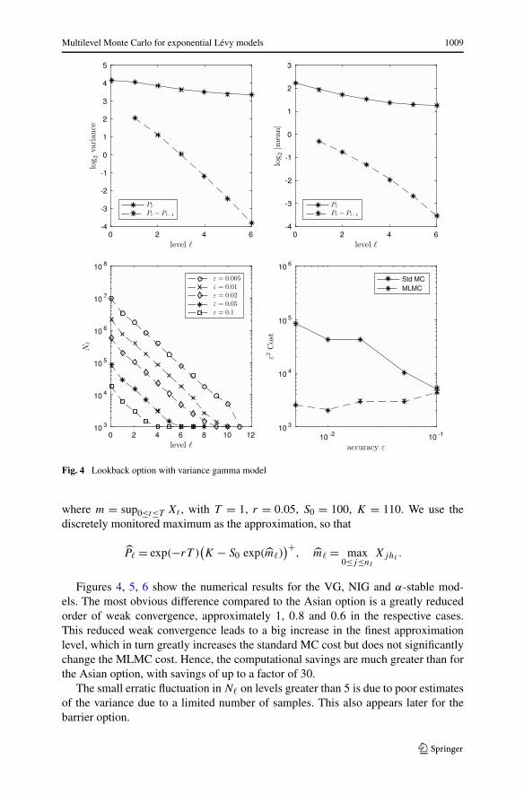
The current code is based on Giles’ MATLAB code [17], using which we generatestandardised numerical results and a set of four figures. The top two plots correspondto a set of experiments to investigate how the variance and mean for both P� andP� − P�−1 vary with level �. The top left plot shows the values for log2 variance, sothat the absolute value of the slope of the line for log2 V[P� − P�−1] indicates theconvergence rate β of V� in condition iii) of Theorem 2.1. Similarly, the absolutevalue of the slope of the line for log2 |E[P� − P�−1]| in the top right plot indicates theweak convergence rate α in the condition i) of Theorem 2.1.
The bottom two plots correspond to a set of MLMC calculations for different val-ues of the desired accuracy ε. Each line in the bottom left plot corresponds to onemultilevel calculation and displays the number of samples N� on each level. Notethat as ε is varied, the MLMC algorithm automatically decides how many levelsare required to reduce the weak error appropriately. The optimal number of sampleson each level is based on an empirical estimation of the multilevel correction vari-ance V�, together with the use of a Lagrange multiplier to determine how best tominimise the overall computational cost for a given target accuracy. A complete de-scription of the algorithm is given in [19, Sect. 3.1, Algorithm 1]. The bottom rightplots show the variation of the computational complexity C with the desired accu-racy ε. In the best cases, the MLMC complexity is O(ε−2), and therefore the plotis of ε2 C versus ε so that we can see whether this is achieved, and compare thecomplexity to that of the standard Monte Carlo method.
6.1 Asian option
The Asian option we consider is an arithmetic Asian call option with discountedpayoff
P = exp(−rT ) max(0, S − K),

1006 M.B. Giles, Y. Xia
where T = 1, r = 0.05, S0 = 100, K = 100 and
S = S0 T −1∫ T
0exp (Xt )dt.
For a general Lévy process, it is not easy to directly sample the integral process. Weuse the trapezoidal approximation
S := S0 T −1n−1∑j=0
1
2h(
exp(Xjh) + exp(X(j+1)h)),
where n = T/h is the number of timesteps. The payoff approximation is then
P = exp(−rT ) max(0, S − K).
Fig. 1 Asian option in variance gamma model

Multilevel Monte Carlo for exponential Lévy models 1007
Fig. 2 Asian option in normal inverse Gaussian model
In the multilevel estimator, the approximation P� on level � is obtained using n� := 2�
timesteps.Figures 1, 2, 3 are for the VG, NIG and α-stable models, respectively. The nu-
merical results in the top right plots indicate approximately second order weakconvergence. With the standard Monte Carlo method, the top left plots showthat the variance is approximately independent of the level, or equivalently thetimestep, and therefore, the standard Monte Carlo calculation has computational costO(ε−2n�) = O(ε−2.5). Multiplying this cost by ε2 to create the bottom right com-plexity plots, the scaled cost is O(n�) and therefore goes up in steps as ε is reduced,when decreasing ε requires an increase in the value of the finest level L. On the otherhand, the convergence rate of the variance of the MLMC estimator is approximately1.2 for VG, 2.0 for NIG and 2 for the α-stable model. Since in all three cases we haveβ > 1, the MLMC theorem gives a complexity which is O(ε−2) which is consistent

1008 M.B. Giles, Y. Xia
Fig. 3 Asian option in spectrally negative α-stable model
with the results in the bottom right plots which show little variation in ε2 C for theMLMC estimator.
For this Asian option, MLMC is 3–8 times more efficient than standard MC. Thegains are modest because the high rate of weak convergence means that only 4 levelsof refinement are required in most cases, so there is only a 24 = 16 difference in costbetween each MC path calculation on the finest level, and each of the MLMC pathcalculations on the coarsest level.
6.2 Lookback option
The lookback option we consider is a put option on the floating underlying,
P = exp(−rT )
(K − sup
0≤t≤T
St
)+= exp(−rT )
(K − S0 exp(m)
)+,
Multilevel Monte Carlo for exponential Lévy models 1009
Fig. 4 Lookback option with variance gamma model
where m = sup0≤t≤T Xt , with T = 1, r = 0.05, S0 = 100, K = 110. We use thediscretely monitored maximum as the approximation, so that
P� = exp(−rT )(K − S0 exp(m�)
)+, m� = max
0≤j≤n�
Xjh�.
Figures 4, 5, 6 show the numerical results for the VG, NIG and α-stable mod-els. The most obvious difference compared to the Asian option is a greatly reducedorder of weak convergence, approximately 1, 0.8 and 0.6 in the respective cases.This reduced weak convergence leads to a big increase in the finest approximationlevel, which in turn greatly increases the standard MC cost but does not significantlychange the MLMC cost. Hence, the computational savings are much greater than forthe Asian option, with savings of up to a factor of 30.
The small erratic fluctuation in N� on levels greater than 5 is due to poor estimatesof the variance due to a limited number of samples. This also appears later for thebarrier option.

1010 M.B. Giles, Y. Xia
Fig. 5 Lookback option with normal inverse Gaussian model
6.3 Barrier option
The barrier option is an up-and-out call with payoff
P = exp(−rT ) (ST − K)+ 1{sup0≤t≤T S(t)<B} = exp(−rT ) (ST − K)+ 1{m<log(B/S0)},
with T = 1, r = 0.05, S0 = 100, K = 100, B = 115. The discretely monitored ap-proximation is
P� = exp(−rT ) (ST − K)+ 1{m�<log(B/S0)}, m� = max0≤j≤n�
Xjh�
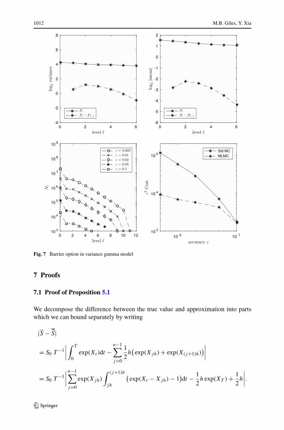
With the barrier option (Figs. 7, 8, 9), the most noticeable change from the previ-ous options is a reduction in the rate of convergence β of the MLMC variance, withβ ≈ 0.75,0.5,0.6 in the three cases. For β < 1, the MLMC theorem proves a com-plexity which is O(ε−2−(1−β)/α), with α here being the rate of weak convergence.The fact that the MLMC complexity is not O(ε−2) is clearly visible from the bottom
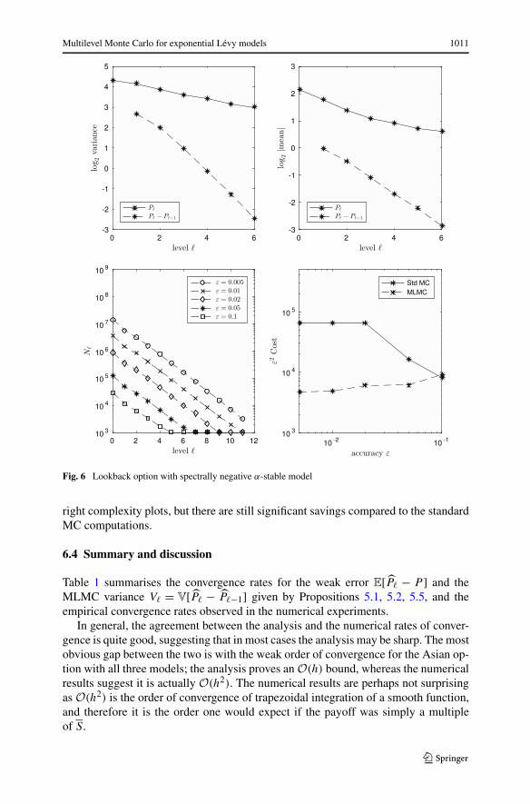
Multilevel Monte Carlo for exponential Lévy models 1011
Fig. 6 Lookback option with spectrally negative α-stable model
right complexity plots, but there are still significant savings compared to the standardMC computations.
6.4 Summary and discussion
Table 1 summarises the convergence rates for the weak error E[P� − P ] and theMLMC variance V� = V[P� − P�−1] given by Propositions 5.1, 5.2, 5.5, and theempirical convergence rates observed in the numerical experiments.
In general, the agreement between the analysis and the numerical rates of conver-gence is quite good, suggesting that in most cases the analysis may be sharp. The mostobvious gap between the two is with the weak order of convergence for the Asian op-tion with all three models; the analysis proves an O(h) bound, whereas the numericalresults suggest it is actually O(h2). The numerical results are perhaps not surprisingas O(h2) is the order of convergence of trapezoidal integration of a smooth function,and therefore it is the order one would expect if the payoff was simply a multipleof S.
1012 M.B. Giles, Y. Xia
Fig. 7 Barrier option in variance gamma model
7 Proofs
7.1 Proof of Proposition 5.1
We decompose the difference between the true value and approximation into partswhich we can bound separately by writing
|S − S|
= S0 T −1∣∣∣∣∫ T
0exp(Xt )dt −
n−1∑j=0
1
2h(
exp(Xjh) + exp(X(j+1)h))∣∣∣∣
= S0 T −1∣∣∣∣n−1∑j=0
exp(Xjh)
∫ (j+1)h
jh
(exp(Xt − Xjh) − 1
)dt − 1
2h exp(XT ) + 1
2h
∣∣∣∣.

Multilevel Monte Carlo for exponential Lévy models 1013
Fig. 8 Barrier option in normal inverse Gaussian model
If we define
bj = exp(Xjh),
Ij =∫ (j+1)h
jh
(exp(Xt − Xjh) − 1
)dt,
RA = −1
2h exp(XT ) + 1
2h,
then
E[(S − S)2] = T −2S2
0 E
[∣∣∣∣n−1∑j=0
bj Ij + RA
∣∣∣∣2]
≤ 2T −2S20
(E
[∣∣∣∣n−1∑j=0
bj Ij
∣∣∣∣2]
+E[R2A])
.

1014 M.B. Giles, Y. Xia
Fig. 9 Barrier option in spectrally negative α-stable model
We have E[R2A] = O(h2), and due to the independence of bj and Ij , we obtain
E
[∣∣∣∣n−1∑j=0
bj Ij
∣∣∣∣2]
= E
[ n−1∑j=0
b2j I
2j + 2
n−1∑m=1
m−1∑j=0
bmImbj Ij
]
=n−1∑j=0
E[b2j ]E[I 2
j ] + 2n−1∑m=1
m−1∑j=0
E[bmImbj Ij ]. (7.1)
Defining A = 2m + ∫(e2z − 1 − 2z1{|z|<1})ν(dz), we have E[b2
j ] = eAjh. Further-more, by the Cauchy–Schwarz inequality,
E[I 2j ] ≤ h E
[∫ (j+1)h
jh
(exp(Xt − Xjh) − 1
)2dt
]
= h
∫ h
0E[(
exp(Xt ) − 1)2]dt
= h
(1
A(eAh − 1 − Ah) − 2
1
r(erh − 1 − rh)
).

Multilevel Monte Carlo for exponential Lévy models 1015
Table 1 Convergence rates ofweak error and variance V� forVG, NIG and α-stableprocesses; δ can be any smallpositive constant. The numericalvalues are estimates based onthe numerical experiments
Option VG
numerical analysis
weak var weak var
Asian O(h2) O(h2) O(h) O(h2)
lookback O(h) O(h1.2) O(h| logh|) O(h)
barrier O(h0.8) O(h0.9) O(h1−δ) O(h1−δ)
Option NIG
numerical analysis
weak var weak var
Asian O(h2) O(h2) O(h) O(h2)
lookback O(h0.8) O(h1.2) O(h1−δ) O(h| logh|)barrier O(h0.4) O(h0.5) O(h0.5−δ) O(h0.5−δ)
Option spectrally negative α-stable with α > 1
numerical for α = 1.5597 analysis
weak var weak var
Asian O(h2) O(h2) O(h) O(h2)
lookback O(h0.6) O(h1.6) O(h1/α−δ) O(h2/α−δ)
barrier O(h0.5) O(h0.6) O(h1/α−δ) O(h1/α−δ)
Note that 1 + x < ex < 1 + x + x2 for 0 < x < 1, and therefore for h < 1/A, we haveE[I 2
j ] < Ah3 and hence
n−1∑j=0
E[b2j ]E[I 2
j ] < Ah3n−1∑j=0
eAjh = AeAT − 1
eAh − 1h3 < (eAT − 1) h2.
Now we calculate the second term in (7.1). Note that for m > j , Im is independentof bmbj Ij , and bm/bj+1 is independent of bj+1bj Ij , so
n−1∑m=1
m−1∑j=0
E[bmImbj Ij ] =n−1∑m=1
E[Im]m−1∑j=0
E[bm/bj+1]E[bj+1bj Ij ].
Firstly, for h < 1/r ,
E[Im] =∫ h
0(ert − 1) dt = r−1(erh − 1 − rh) < r h2.
1016 M.B. Giles, Y. Xia
Moreover, we have E[bm/bj+1] = er(m−j−1)h and
E[bj+1bj Ij ] = E
[exp(2Xjh) exp(X(j+1)h − Xjh)
×∫ (j+1)h
jh
(exp(Xt − Xjh) − 1
)dt
]
= E[exp(2Xjh)] E[
exp(Xh)
∫ h
0
(exp(Xt ) − 1
)dt
]
= eAjh
∫ h
0
(E[exp(Xh − Xt)]E[exp(2Xt)] −E[exp(Xh)]
)dt
= eAjh
∫ h
0(er(h−t)eAt − erh) dt
= eAjherh e(A−r)h − 1 − (A − r)h
A − r.
Thus, for h < 1/(A − r),
n−1∑m=1
m−1∑j=0
E[bm/bj+1]E[bj+1bj Ij ] = e(A−r)h − 1 − (A − r)
A − r
n−1∑m=1
m−1∑j=0
er(m−j)heAjh
= e(A−r)h − 1 − (A − r)h
(A − r) (e(A−r)h − 1)
n−1∑m=1
(eAmh − ermh)
< heAT − 1
eAh − 1
< A−1(eAT − 1).
Hence,
E
[ n−1∑m=1
m−1∑j=0
bmImbj Ij
]=
n−1∑m=1
E[Im]m−1∑j=0
E[bm/bj+1]E[bj+1bj Ij ] = O(h2),
and we can therefore conclude that E[(S − S)2] = O(h2). �
7.2 Lévy process decomposition
The proofs rely on a decomposition of the Lévy process into a combination of a finiteactivity pure jump part, a drift part, and a residual part consisting of very small jumps.
Let X be an (m,0, ν)-Lévy process, i.e.,
Xt = mt +∫ t
0
∫{|z|≥1}
z J (dz,ds) +∫ t
0
∫{|z|<1}
z(J (dz,ds) − ν(dz)ds
).

Multilevel Monte Carlo for exponential Lévy models 1017
The finite activity jump part is defined by
Xεt =
∫ t
0
∫{ε<|z|}
z J (dz,ds) =Nt∑i=1
Yi,
which is the compound Poisson process truncating the jumps of X smaller than ε,which is assumed to satisfy 0 < ε < 1. The intensity of (Nt ) and the c.d.f. of Yi
are
λε =∫
{ε<|z|}ν(dz),
P[Yi < y
] = λ−1ε
∫{z<y}
1{ε<|z|}ν(dz).
The drift rate for the drift term is defined to be
με = m −∫
{ε<|z|<1}z ν(dz),
so that the residual term is then a martingale, given by
Rεt :=
∫ t
0
∫{|z|≤ε}
z(J (dz,ds) − ν(dz)ds
).
We define
σ 2ε =
∫{|z|≤ε}
z2ν(dz), (7.2)
so that V[Rεt ] = σ 2
ε t . The three quantities με , λε and σε all play a major role in thesubsequent numerical analysis.
We bound Dn by the difference between continuous maxima and 2-point maximaover all timesteps via
Dn = sup0≤t≤1
Xt − maxi=0,1,...,n
X in
≤ maxi=0,...,n−1
D(i)n ,
where the random variables
D(i)n = sup
[ in, i+1
n]Xt − max
(Xi+1
n,X i
n
)
are independent and identically distributed. If we now define
�(i)Xt = X in+t
− X in, �(i)Xε
t = Xεin+t
− Xεin
,
�(i)t = t − in, �(i)Rε
t = Rεin+t
− Rεin
,

1018 M.B. Giles, Y. Xia
then
D(i)n = sup
[0, 1n]�(i)Xt − (�(i)X 1
n)+
= sup[0, 1
n](�(i)Xε
t + �(i)Rεt + με�
(i)t) −(
�(i)Xε1n
+ �(i)Rε1n
+ με
1
n
)+
≤ sup[0, 1
n](�(i)Xε
t + �(i)Rεt ) − (�(i)Xε
1n
+ �(i)Rε1n
)+ + |με|n
≤ sup[0, 1
n]�(i)Xε
t − (�(i)Xε1n
)+ + |με|n
+ sup[0, 1
n]�(i)Rε
t + (−�(i)Rε1n
)+
≤ sup[0, 1
n]�(i)Xε
t − (�(i)Xε1n
)+ + |με|n
+ 2 sup[0, 1
n]|�(i)Rε
t |, (7.3)
where we use (a + b)+ ≤ a+ + b+ with a = �(i)Xε1n
+ �(i)Rε1n
+ με1n
, b = −με1n
in
the first inequality, and a = �(i)Xε1n
+ �(i)Rε1n
, b = −�(i)Rε1n
in the second.
Let Z(i)n := sup[0, 1
n] �
(i)Xεt − (�Xε
1n
)+ and S(i)n := sup[0, 1
n] |�(i)Rε
t |. Then for
p ≥ 1, Jensen’s inequality gives
E[Dpn ] ≤ E
[max
0≤i<n(Z(i)
n + |με|n
+ 2S(i)n )p
]
≤ 3p−1E
[max
0≤i<n(Z(i)
n )p + (|με|/n)p + 2p max0≤i<n
(S(i)n )p
]
≤ 3p−1n E
[(sup[0, 1
n]Xε
t − (Xε1n
)+)p]+ 3p−1(|με|/n)p
+3p−12pE
[max
0≤i<n(S(i)
n )p], (7.4)
where in the final step we have used the fact that all of the �(i)Xεt have the same
distribution as Xεt .
The task now is to bound the first and third terms in the final line of (7.4).
7.3 Bounding moments of sup[0, 1n ] X
εt − (Xε
1n
)+
Theorem 7.1 Let X be a scalar Lévy process with triple (m,0, ν), and let Xεt , με ,
λε and σε be defined as in Sect. 7.2. Then provided λε ≤ n, for any p > 1, there exists

Multilevel Monte Carlo for exponential Lévy models 1019
Fig. 10 Behaviour of (Xεt ) in the case of one or two jumps in the interval [0, 1
n ]
a constant Kp such that
E
[(sup[0, 1
n]Xε
t − (Xε1n
)+)p] ≤ Kp
(εp + Lε(p)
λ2ε
)λ2
ε
n2, (7.5)
where Lε (p) = p∫{x>ε} x
p−1λ2x dx is a function depending on the Lévy measure
ν(x).
Proof Let
Z = sup[0, 1
n]Xε
t − (Xε1n
)+.
We determine an upper bound on E[Zp] by analysing the jump behaviour of the finiteactivity process (Xε
t ) in a single interval [0, 1n].
Let N be the number of jumps. If N ≤ 1, then Z = 0, while if N = 2, thenZ ≤ min (|Y1| , |Y2|). This can be seen from the behaviour of (Xε
t ) in the differentscenarios illustrated in Fig. 10. More generally, if N = k, k ≥ 2, then
Z > x =⇒ ∃ 1 ≤ j ≤ k − 1 such that
∣∣∣∣j∑
�=1
Y�
∣∣∣∣ > x,
∣∣∣∣k∑
�=j+1
Y�
∣∣∣∣ > x
=⇒ ∃ j1, j2 such that |Yj1 | >x
k − 1, |Yj2 | >
x
k − 1.
Since
P
[∃j1, j2 such that |Yj1 | >
x
k − 1, |Yj2 | >
x
k − 1
]
≤∑
(j1,j2)
P
[|Yj1 | >
x
k − 1, |Yj2 | >
x
k − 1
]
= k(k − 1)
2P
[|Y1| > x
k − 1
]2
,

1020 M.B. Giles, Y. Xia
it follows that
E[Zp | N = k] = p
∫xp−1
P[Z > x | N = k]dx
≤ k (k − 1)
2p
∫xp−1
P
[|Y1| > x
k − 1
]2
dx
= k (k − 1)
2
p
λ2ε
∫xp−1
(∫{|z|>x/(k−1)}
1{ε<|z|}ν(dz)
)2
dx
= k (k − 1)p+1
2
p
λ2ε
∫xp−1
(∫{|z|>x}
1{ε<|z|}ν(dz)
)2
dx
=: dk,p
(εp + Lε(p)
λ2ε
),
where dk,p = 12k (k − 1)p+1. We then have
E[Zp] =∞∑
k=2
E[Zp | N = k] P[N = k]
≤(
εp + Lε(p)
λ2ε
)exp
(− λε
n
) ∞∑k=2
dk,p
(λε
n
)k 1
k! .
For kp = �p� + 2, there exists Cp such that for any k ≥ kp , dk,p ≤ Cpk!
(k−kp)! , so
∞∑k=2
dk,p
(λε
n
)k 1
k! ≤kp−1∑k=2
dk,p
(λε
n
)k 1
k! + Cp
∞∑k=kp
(λε
n
)k 1
(k − kp)!
≤kp−1∑k=2
dk,p
(λε
n
)k 1
k! + Cp
(λε
n
)k
p
exp
(λε
n
)
≤ Kp
(λε
n
)2
for some constant Kp , where the last step uses the fact that λε ≤ n. Therefore, weobtain the final result that
E[Zp] ≤ Kp
(εp + Lε(p)
λ2ε
)λ2
ε
n2. �
7.4 Bounding moments of sup[0,T ] |Rεt |
Proposition 7.1 Let X be a scalar Lévy process with triple (m,0, ν) and let Rεt , με ,
λε and σε be defined as in Sect. 7.2. Then (Rεt ) satisfies
E
[sup[0,T ]
|Rεt |p
]≤
{Kp(T p/2σ
pε + T
∫{|z|≤ε} |z|pν(dx)), p > 2,
Kp T p/2σpε , 1 ≤ p ≤ 2,
where Kp is a constant depending on p.
Multilevel Monte Carlo for exponential Lévy models 1021
Proof For any 1 ≤ p ≤ 2, by Jensen’s inequality and the Doob inequality,
E
[sup
0≤t≤T
|Rεt |p
]≤ E
[sup
0≤t≤T
|Rεt |2
]p/2
≤ 2pE[|Rε
T |2]p/2 = 2p T p/2σpε .
For any p > 2, the Burkholder–Davis–Gundy inequality gives
E
[sup
0≤t≤1|Rε
t |p]
≤ E[[Rε]p/2
1
],
where[Rε
]t
is the quadratic variation of Rεt . We can use the method in the proof of
[24, Theorem V.66] to get
E[[Rε]p/2
1
] ≤ Kp
[(∫{|z|≤ε}
z2ν(dz)
)p/2
+∫
{|z|≤ε}|z|pν(dz)
]
= Kp
(σp
ε +∫
{|z|≤ε}|z|pν(dz)
),
where Kp is a constant depending on p.To extend this result to an arbitrary time interval [0, T ], we use a change of time
coordinate t ′ = t/T with associated changed Lévy measure ν′(dz) = T ν(dz) to ob-tain
E
[sup[0,T ]
|Rεt |p
]≤ Kp
[T p/2σp/2
ε + T
∫{|z|≤ε}
|z|pν(dz)
]. �
7.5 Bounding moments of max0≤i<n S(i)n
Proposition 7.2 Let X be a scalar pure jump Lévy process, with Lévy measure ν(x)
which satisfies
C2 |x|−1−α ≤ ν(x) ≤ C1 |x|−1−α for |x| ≤ 1,
for constants C1,C2 > 0 and 0 ≤ α < 2. If S(i)n is defined as in Sect. 7.2 and λε ≤ n,
then for p ≥ 1 and arbitrary δ > 0, there exists a constant Cp,δ , which does notdepend on n, ε, such that
E
[(max
0≤i<nS(i)
n
)p]≤ Cp,δ εp−δ.
In the particular case of α = 0, such a bound holds with δ = 0.
Proof By Proposition 7.1, for q > 2,
E
[(max
0≤i<nS(i)
n
)q]≤ n E
[sup[0, 1
n]|Rε
t |q]
≤ Kq
(n1−q/2σq
ε +∫
{|z|≤ε}|z|q ν(dx)
).

1022 M.B. Giles, Y. Xia
Recalling the definition of σε in (7.2), due to the assumption on ν(x), we have
σqε ≤
(2C1
2 − α
)q/2
εq−qα/2,
∫{|z|≤ε}
|z|q ν(dx) ≤ 2C1
q − αεq−α.
Given p ≥ 1, for any q > max (2,p), Jensen’s inequality gives
E
[(max
0≤i<nS(i)
n
)p]≤ E
[(max
0≤i<nS(i)
n
)q]p/q
≤ Kp/qq
[(2C1
2 − α
)q/2 (ε−α
n
)q/2−1
+ 2C1
q − α
]p/q
εp−αp/q .
If α = 0, then the desired bound is obtained immediately. On the other hand, if0 < α < 2, then
λε ≥ C2
∫{ε<|z|<1}
1
|z|α+1dz = 2C2
α(ε−α − 1).
Since λε ≤ n, this implies that ε−α ≤ Kα2C2
n + 1, and thus ε−α/n is bounded. Hencethere exists a constant C such that
E
[(max
0≤i<nS(i)
n
)p]≤ C εp−αp/q,
and by choosing q large enough so that αp/q ≤ δ, we obtain the desired bound. �
7.6 Proof of Theorem 4.2
Provided λε ≤ n, by (7.4) and (7.5) we have
E[Dpn ] ≺ E
[(max
0≤i<nS(i)
n
)p]︸ ︷︷ ︸
1)
+ εp λ2ε
n︸ ︷︷ ︸2)
+ Lε (p)
n︸ ︷︷ ︸3)
+( |με|
n
)p
︸ ︷︷ ︸4)
, (7.6)
where the notation u ≺ v means that there exists a constant c > 0 independent of n
such that u < cv.We can now bound each term, given the specification of the Lévy measure, and
if we can choose appropriately how ε → 0 as n → ∞ so that the RHS of (7.6) isconvergent, then the convergence rate of E[Dp
n ] can be bounded.For 0 < x < 1,
λx ≤ C1
∫{x<|z|<1}
1
|z|α+1dz +
∫{1<|z|}
exp (−C3 |z|) dz
≤{
2C1 log 1x
+ �1, α = 0,
�2 x−α, 0 < α < 2,(7.7)

Multilevel Monte Carlo for exponential Lévy models 1023
where �1, �2 are constants with �2 ≥ 2C−13 , while for x ≥ 1,
λx ≤∫
{x<|z|}exp (−C3 |z|) dz = 2C−1
3 exp(−C3 x).
If α > 0, then
Lε(p) = p
∫{x>ε}
xp−1λ2x dx
≤ �22 p
∫{x>ε}
xp−1(1{x<1}x−2α + 1{x>1} exp(−2C3x))dx
≤
⎧⎪⎨⎪⎩
�3, p > 2α,
�3 log 1ε
+ �4, p = 2α,
�3ε−2α+p + �4, p < 2α,
(7.8)
where �3 and �4 are additional constants. If α = 0, it is easily verified that Lε(p) isbounded for p ≥ 1, so (7.8) applies equally to this case.
Given 0 < ε < 1, we have
|με| =∣∣∣∣m −
∫ε<|z|<1
z ν(dz)
∣∣∣∣ ≤{
|m| + |C1 − C2| ε1−α−1α−1 , α �= 1,
|m| + |C1 − C2| log 1ε, α = 1.
(7.9)
Subject to the condition that λε ≤ n, we now consider the terms in (7.6).
1. By Proposition 7.2,
E
[(max
0≤i<nS(i)
n
)p]≺ εp−δ, for any δ > 0.
2. By (7.7),
εp λ2ε
n≺ n−1 ×
{εp log 1
ε, α = 0,
εp−2α, 0 < α < 2.
3. By (7.8),
Lε(p)
n≺ n−1 ×
⎧⎪⎨⎪⎩
1, p > 2α,
log 1ε, p = 2α,
ε−2α+p, p < 2α.
4. By (7.9),
( |με|n
)p
≺ n−p ×
⎧⎪⎨⎪⎩
1 + |C1 − C2|pεp(1−α), α > 1,
1 + (|C1 − C2| log 1ε)p, α = 1,
1, α < 1.
In the following, we assume C1 �= C2.

1024 M.B. Giles, Y. Xia
Suppose p ≥ 2α. If we choose ε = C n−2/p , then λε ≺ ε−α ≺ n2α/p , and the con-stant C can be taken to be sufficiently small so that λε ≤ n for sufficiently large n.Taking δ < p/2, we find that the dominant contribution to (7.6) comes from 3), givingthe desired result that
E[Dpn ] ≺
{n−1, p > 2α,
logn/n, p = 2α.
If 1 ≤ p < 2α, Hölder’s inequality gives E[Dpn ] ≤ E[D2α
n ] p2α ≺ (logn/n)
p2α .
For a spectrally negative process, sup[0, 1n] X
εt − (Xε
1n
)+ = 0, since X does not have
positive jumps, and hence
E[Dpn ] ≤ E
[(max
0≤i<nS(i)
n
)p]+
( |με|n
)p
.
We can take ε = Cn−1/α with the constant C again chosen so that λε ≤ n for suffi-ciently large n. We then obtain
E[Dpn ] ≺
{n−p/α+δ, α ≥ 1,
n−p, α < 1,
for any δ > 0. �
7.7 Proof of Proposition 5.4
We decompose the term we want to bound into parts and then balance their asymp-totic orders to get the desired result.
Note that 1{mn<B} − 1{m<B} = 1 only if either m is close to the barrier or thedifference between discretely and continuously monitored maximum Dn = m − mn
is large. More precisely,
{1{mn<B} − 1{m<B} = 1
} ⊆ F ∪ G,
where F := {B ≤ m ≤ B +n−r} and G := {Dn > n−r} for an r > 0 to be determined.Hence
E[1{mn<B} − 1{m<B}] ≤ P[F ] + P[G].Due to the locally bounded density for m, P[F ] = O(n−r ). If we denote
Z(i)n = sup
[0, 1n]�(i)Xε
t − (�(i)Xε1n
)+,
where �(i)Xt is defined as previously in Sect. 7.2, then (7.3) gives
Dn ≤ max0≤i<n
Z(i)n + |με|
n+ max
0≤i<nS(i)
n .

Multilevel Monte Carlo for exponential Lévy models 1025
For α < 1, με is bounded, so |με| ≤ 12n1−r for sufficiently large n. Hence,
P[Dn > n−r ] ≤ P
[max
0≤i<nZ(i)
n + max0≤i<n
S(i)n >
1
2n−r
]
≤ P
[max
0≤i<nZ(i)
n >1
4n−r
]+ P
[max
0≤i<nS(i)
n >1
4n−r
].
Now, max0≤i<n Z(i)n > 0 requires that there are at least two jumps in one of the n
intervals. The probability of two jumps in one particular interval is
1 − exp
(−λε
n
)(1 + λε
n
)≺
(λε
n
)2
if λε ≤ n, and hence
P
[max
0≤i<nZ(i)
n >1
4n−r
]≺ λ2
ε
n.
We use the Markov inequality for the remaining term. According to Proposition 7.1,E[max0≤i<n(S
(i)n )p] ≺ εp−δ and so
P
[max
0≤i<nS(i)
n >1
4n−r
]≺ E
[max
0≤i<n(S(i)
n )p] / (
1
4n−r
)p
≺ εp−δnrp.
Combining these elements, provided λε ≤ n, we have
E[1{mn<B} − 1{m<B}] ≺ n−r + εp−δnrp + λ2ε
n.
Equating the first two terms on the right-hand side gives ε = n−r(1+p)/(p−δ).If α = 0, then λε ≺ log 1
ε≺ logn, so λε = O(n) is satisfied. We also have
λ2ε
n≺ (logn)2
n, and therefore for any r < 1, we have E[1{mn<B} − 1{m<B}] ≺ n−r .
If 0 < α < 2, then λε ≺ ε−α ≺ nrα(1+p)/(p−δ), and hence we obtain thatλ2
ε
n≺ n−1+2rα(1+p)/(p−δ). Balancing n−r and n−1+2rα(1+p)/(p−δ) gives λε = O(n)
and
r =(
1 + 2α1 + p
p − δ
)−1
. (7.10)
Since r → 11+2α
as δ → 0, and p → ∞, for any fixed value of r < 11+2α
, it is possibleto choose appropriate values of p and δ to satisfy (7.10) and thereby conclude thatE[1{mn<B} − 1{m<B}] ≺ n−r . �
Acknowledgements This work was supported by the China Scholarship Council and the Oxford–ManInstitute of Quantitative Finance. We should like to thank Ben Hambly, Andreas Kyprianou, Loïc Chau-mont, Jacek Małecki and Jose Blanchet for their helpful comments.
Open Access This article is distributed under the terms of the Creative Commons Attribution 4.0 Inter-national License (http://creativecommons.org/licenses/by/4.0/), which permits unrestricted use, distribu-tion, and reproduction in any medium, provided you give appropriate credit to the original author(s) andthe source, provide a link to the Creative Commons license, and indicate if changes were made.

1026 M.B. Giles, Y. Xia
References
1. Asmussen, S., Glynn, P., Pitman, J.: Discretization error in simulation of one-dimensional reflectingBrownian motion. Ann. Appl. Probab. 5, 875–896 (1995)
2. Avikainen, R.: Convergence rates for approximations of functionals of SDEs. Finance Stoch. 13, 381–401 (2009)
3. Blanchet, J.: Personal communication (2015)4. Carr, P., Wu, L.: The finite moment log stable process and option pricing. J. Finance 58, 753–778
(2003)5. Chambers, J.M., Mallows, C.L., Stuck, B.: A method for simulating stable random variables. J. Am.
Stat. Assoc. 71, 340–344 (1976)6. Chaumont, L.: On the law of the supremum of Lévy processes. Ann. Probab. 41, 1191–1217 (2013)7. Chaumont, L., Małecki, J.: The asymptotic behavior of the density of the supremum of Lévy pro-
cesses. Ann. Inst. Henri Poincaré Probab. Stat. 52, 1178–1195 (2016)8. Chen, A.: Sampling Error of the Supremum of a Lévy Process. Ph.D. Thesis, University of Illinois at
Urbana-Champaign (2011). Available online at https://www.ideals.illinois.edu/handle/2142/263219. Chen, A., Feng, L., Song, R.: On the monitoring error of the supremum of a normal jump diffusion
process. J. Appl. Probab. 48, 1021–1034 (2011)10. Cont, R., Tankov, P.: Financial Modelling with Jump Processes. Chapman & Hall/CRC Press, London
(2004)11. Dereich, S.: Multilevel Monte Carlo algorithms for Lévy-driven SDEs with Gaussian correction. Ann.
Appl. Probab. 21, 283–311 (2011)12. Dereich, S., Heidenreich, F.: A multilevel Monte Carlo algorithm for Lévy-driven stochastic differen-
tial equations. Stoch. Process. Appl. 121, 1565–1587 (2011)13. Dia, E., Lamberton, D.: Connecting discrete and continuous lookback or hindsight options in expo-
nential Lévy models. Adv. Appl. Probab. 43, 1136–1165 (2011)14. Ferreiro-Castilla, A., Kyprianou, A.E., Scheichl, R., Suryanarayana, G.: Multilevel Monte Carlo sim-
ulation for Lévy processes based on the Wiener–Hopf factorisation. Stoch. Process. Appl. 124, 985–1010 (2014)
15. Figueroa-López, J., Tankov, P.: Small-time asymptotics of stopped Lévy bridges and simulationschemes with controlled bias. Bernoulli 20, 1126–1164 (2014)
16. Giles, M.B.: Improved multilevel Monte Carlo convergence using the Milstein scheme. In: Keller,A., et al. (eds.) Monte Carlo and Quasi-Monte Carlo Methods 2006, pp. 343–358. Springer, Berlin(2007)
17. Giles, M.B.: Multilevel Monte Carlo path simulation. Oper. Res. 56, 607–617 (2008)18. Giles, M.B.: Multilevel Monte Carlo methods. In: Dick, J., et al. (eds.) Monte Carlo and Quasi-Monte
Carlo Methods 2012, pp. 83–103. Springer, Berlin (2012)19. Giles, M.B.: Multilevel Monte Carlo methods. Acta Numer. 24, 259–328 (2015)20. Kuznetsov, A.: On extrema of stable processes. Ann. Probab. 39, 1027–1060 (2011)21. Kuznetsov, A., Kyprianou, A., Pardo, J., Van Schaik, K.: A Wiener–Hopf Monte Carlo simulation
technique for Lévy processes. Ann. Appl. Probab. 21, 2171–2190 (2011)22. Kwasnicki, M., Małecki, J., Ryznar, M.: Suprema of Lévy processes. Ann. Probab. 41, 2047–2065
(2013)23. Kyprianou, A.: Introductory Lectures on Fluctuations of Lévy Processes with Applications. Springer,
Berlin (2006)24. Protter, P.: Stochastic Integration and Differential Equations, 2nd edn. Springer, Berlin (2004)25. Schoutens, W.: Lévy Processes in Finance: Pricing Financial Derivatives. Wiley/Blackwell, New Jer-
sey (2003)26. Spitzer, F.: A combinatorial lemma and its application to probability theory. Trans. Am. Math. Soc.
82, 323–339 (1956)


![Lévy Processes and Lévy White Noise as Tempered Distributions · arXiv:1509.05274v1 [math.PR] 17 Sep 2015 Lévy Processes and Lévy White Noise as Tempered Distributions Robert](https://static.fdocuments.us/doc/165x107/5c4bf79693f3c31436469ec3/levy-processes-and-levy-white-noise-as-tempered-distributions-arxiv150905274v1.jpg)


![On the Performance of Delta Hedging Strategies in ... › pdf › 0911.4859.pdf · exponential Lévy models, this has been done in the unpublished thesis [10] for continuous time](https://static.fdocuments.us/doc/165x107/5f25b5c37c2e7b5a02308c37/on-the-performance-of-delta-hedging-strategies-in-a-pdf-a-09114859pdf.jpg)


