Multilabel Things

1

A Review on Multi-Label Learning Algorithms

Min-Ling Zhang and Zhi-Hua Zhou, Fellow, IEEE

Abstract

Multi-label learning studies the problem where each example is represented by a single instance

while associated with a set of labels simultaneously. During the past decade, significant amount of

progresses have been made towards this emerging machine learning paradigm. This paper aims to

provide a timely review on this area with emphasis on state-of-the-art multi-label learning algorithms.

Firstly, fundamentals on multi-label learning including formal definition and evaluation metrics are

given. Secondly and primarily, eight representative multi-label learning algorithms are scrutinized under

common notations with relevant analyses and discussions. Thirdly, several related learning settings

are briefly summarized. As a conclusion, online resources and open research problems on multi-label

learning are outlined for reference purposes.

Index Terms

Multi-label learning, label correlations, problem transformation, algorithm adaptation.

I. INTRODUCTION

Traditional supervised learning is one of the mostly-studied machine learning paradigms,

where each real-world object (example) is represented by a single instance (feature vector)

and associated with a single label. Formally, let X denote the instance space and Y denote

the label space, the task of traditional supervised learning is to learn a function f : X → Y

from the training set {(xi, yi) | 1 ≤ i ≤ m}. Here, xi ∈ X is an instance characterizing

the properties (features) of an object and yi ∈ Y is the corresponding label characterizing its

Min-Ling Zhang is with the School of Computer Science and Engineering, and the MOE Key Laboratory of Computer

Network and Information Integration, Southeast University, Nanjing 210096, China. Email: [email protected].

Zhi-Hua Zhou is with the National Key Laboratory for Novel Software Technology, Nanjing University, Nanjing 210023,

China. Email: [email protected]. (Corresponding author)

2

semantics. Therefore, one fundamental assumption adopted by traditional supervised learning is

that each example belongs to only one concept, i.e. having unique semantic meaning.

Although traditional supervised learning is prevailing and successful, there are many learning

tasks where the above simplifying assumption does not fit well, as real-world objects might be

complicated and have multiple semantic meanings simultaneously. To name a few, in text cate-

gorization, a news document could cover several topics such as sports, London Olympics, ticket

sales and torch relay; In music information retrieval, a piece of symphony could convey various

messages such as piano, classical music, Mozart and Austria; In automatic video annotation,

one video clip could be related to some scenarios, such as urban and building, and so on.

To account for the multiple semantic meanings that one real-world object might have, one

direct solution is to assign a set of proper labels to the object to explicitly express its semantics.

Following the above consideration, the paradigm of multi-label learning naturally emerges [95].

In contrast to traditional supervised learning, in multi-label learning each object is also repre-

sented by a single instance while associated with a set of labels instead of a single label. The

task is to learn a function which can predict the proper label sets for unseen instances.1

Early researches on multi-label learning mainly focus on the problem of multi-label text

categorization [63], [75], [97]. During the past decade, multi-label learning has gradually attracted

significant attentions from machine learning and related communities and has been widely applied

to diverse problems from automatic annotation for multimedia contents including image [5], [67],

[74], [85], [102] to bioinformatics [16], [27], [107], web mining [51], [82], rule mining [84],

[99], information retrieval [35], [114], tag recommendation [50], [77], etc. Specifically, in recent

six years (2007-2012), there are more than 60 papers with keyword multi-label (or multilabel)

in the title appearing in major machine learning-related conferences (including ICML/ECML

PKDD/IJCAI/AAAI/KDD/ICDM/NIPS).

1In a broad sense, multi-label learning can be regarded as one possible instantiation of multi-target learning [95], where each

object is associated with multiple target variables (multi-dimensional outputs) [3]. Different types of target variables would

give rise to different instantiations of multi-target learning, such as multi-label learning (binary targets), multi-dimensional

classification (categorical/multi-class targets), multi-output/multivariate regression (numerical targets), and even learning with

combined types of target variables.

3

This paper serves as a timely review on the emerging area of multi-label learning, where

its state-of-the-art is presented in three parts.2 In the first part (Section II), fundamentals on

multi-label learning including formal definition (learning framework, key challenge, threshold

calibration) and evaluation metrics (example-based, label-based, theoretical results) are given. In

the second and primary part (Section III), technical details of up to eight representative multi-label

algorithms are scrutinized under common notations with necessary analyses and discussions. In

the third part (Section IV), several related learning settings are briefly summarized. To conclude

this review (Section V), online resources and possible lines of future researches on multi-label

learning are discussed.

II. THE PARADIGM

A. Formal Definition

1) Learning Framework: Suppose X = Rd (or Zd) denotes the d-dimensional instance space,

and Y = {y1, y2, · · · , yq} denotes the label space with q possible class labels. The task of multi-

label learning is to learn a function h : X → 2Y from the multi-label training set D = {(xi, Yi) |

1 ≤ i ≤ m}. For each multi-label example (xi, Yi), xi ∈ X is a d-dimensional feature vector

(xi1, xi2, · · · , xid)⊤ and Yi ⊆ Y is the set of labels associated with xi.3 For any unseen instance

x ∈ X , the multi-label classifier h(·) predicts h(x) ⊆ Y as the set of proper labels for x.

To characterize the properties of any multi-label data set, several useful multi-label indicators

can be utilized [72], [95]. The most natural way to measure the degree of multi-labeledness

is label cardinality: LCard(D) = 1m

∑m

i=1 |Yi|, i.e. the average number of labels per example;

Accordingly, label density normalizes label cardinality by the number of possible labels in the

2Note that there have been some nice reviews on multi-label learning techniques [17], [89], [91]. Compared to earlier attempts

in this regard, we strive to provide an enriched version with the following enhancements: a) In-depth descriptions on more

algorithms; b) Comprehensive introductions on latest progresses; c) Succinct summarizations on related learning settings.

3In this paper, the term “multi-label learning” is used in equivalent sense as “multi-label classification” since labels assigned

to each instance are considered to be binary. Furthermore, there are alternative multi-label settings where other than a single

instance each example is represented by a bag of instances [113] or graphs [54], or extra ontology knowledge might exist on the

label space such as hierarchy structure [2], [100]. To keep the review comprehensive yet well-focused, examples are assumed

to adopt single-instance representation and possess flat class labels.

4

TABLE I

SUMMARY OF MAJOR MATHEMATICAL NOTATIONS.

Notations Mathematical Meanings

X d-dimensional instance space Rd (or Zd)

Y label space with q possible class labels {y1, y2, · · · , yq}

x d-dimensional feature vector (x1, x2, · · · , xd)⊤ (x ∈ X )

Y label set associated with x (Y ⊆ Y)

Y complementary set of Y in Y

D multi-label training set {(xi, Yi) | 1 ≤ i ≤ m}

S multi-label test set {(xi, Yi) | 1 ≤ i ≤ p}

h(·) multi-label classifier h : X → 2Y , where h(x) returns the set of proper labels for x

f(·, ·) real-valued function f : X × Y → R, where f(x, y) returns the confidence of being proper label of x

rankf (·, ·) rankf (x, y) returns the rank of y in Y based on the descending order induced from f(x, ·)

t(·) thresholding function t : X → R, where h(x) = {y | f(x, y) > t(x), y ∈ Y}

| · | |A| returns the cardinality of set A

[[·]] [[π]] returns 1 if predicate π holds, and 0 otherwise

φ(·, ·) φ(Y, y) returns +1 if y ∈ Y , and −1 otherwise

Dj binary training set {(xi, φ(Yi, yj)) | 1 ≤ i ≤ m} derived from D for the j-th class label yj

ψ(·, ·, ·) ψ(Y, yj , yk) returns +1 if yj ∈ Y and yk /∈ Y , and −1 if yj /∈ Y and yk ∈ Y

Djk binary training set {(xi, ψ(Yi, yj , yk)) | φ(Yi, yj) 6= φ(Yi, yk), 1 ≤ i ≤ m} derived from D for the

label pair (yj , yk)

σY(·) injective function σY : 2Y → N mapping from the power set of Y to natural numbers (σ−1Y being

the corresponding inverse function)

D†Y multi-class (single-label) training set {(xi, σY(Yi)) | 1 ≤ i ≤ m} derived from D

B binary learning algorithm [complexity: FB(m,d) for training; F ′B(d) for (per-instance) testing]

M multi-class learning algorithm [complexity: FM(m, d, q) for training; F ′M(d, q) for (per-instance) testing]

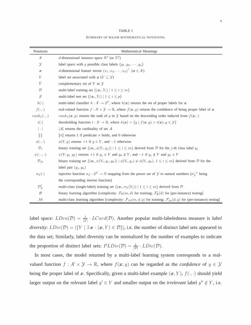
label space: LDen(D) = 1|Y| · LCard(D). Another popular multi-labeledness measure is label

diversity: LDiv(D) = |{Y | ∃x : (x, Y ) ∈ D}|, i.e. the number of distinct label sets appeared in

the data set; Similarly, label diversity can be normalized by the number of examples to indicate

the proportion of distinct label sets: PLDiv(D) = 1|D| · LDiv(D).

In most cases, the model returned by a multi-label learning system corresponds to a real-

valued function f : X × Y → R, where f(x, y) can be regarded as the confidence of y ∈ Y

being the proper label of x. Specifically, given a multi-label example (x, Y ), f(·, ·) should yield

larger output on the relevant label y′ ∈ Y and smaller output on the irrelevant label y′′ /∈ Y , i.e.

5

f(x, y′) > f(x, y′′). Note that the multi-label classifier h(·) can be derived from the real-valued

function f(·, ·) via: h(x) = {y | f(x, y) > t(x), y ∈ Y}, where t : X → R acts as a thresholding

function which dichotomizes the label space into relevant and irrelevant label sets.

For ease of reference, Table I lists major notations used throughout this review along with

their mathematical meanings.

2) Key Challenge: It is evident that traditional supervised learning can be regarded as a

degenerated version of multi-label learning if each example is confined to have only one single

label. However, the generality of multi-label learning inevitably makes the corresponding learning

task much more difficult to solve. Actually, the key challenge of learning from multi-label data

lies in the overwhelming size of output space, i.e. the number of label sets grows exponentially

as the number of class labels increases. For example, for a label space with 20 class labels

(q = 20), the number of possible label sets would exceed one million (i.e. 220).

To cope with the challenge of exponential-sized output space, it is essential to facilitate

the learning process by exploiting correlations (or dependency) among labels [95], [106]. For

example, the probability of an image being labeled annotated with label Brazil would be high if

we know it has labels rainforest and soccer; A document is unlikely to be labeled as entertainment

if it is related to politics. Therefore, effective exploitation of the label correlations information

is deemed to be crucial for the success of multi-label learning techniques. Existing strategies

to label correlations exploitation could among others be roughly categorized into three families,

based on the order of correlations that the learning techniques have considered [106]:

• First-order strategy: The task of multi-label learning is tackled in a label-by-label style and

thus ignoring co-existence of the other labels, such as decomposing the multi-label learning

problem into a number of independent binary classification problems (one per label) [5],

[16], [108]. The prominent merit of first-order strategy lies in its conceptual simplicity and

high efficiency. On the other hand, the effectiveness of the resulting approaches might be

suboptimal due to the ignorance of label correlations.

• Second-order strategy: The task of multi-label learning is tackled by considering pairwise

relations between labels, such as the ranking between relevant label and irrelevant label

6

[27], [30], [107], or interaction between any pair of labels [33], [67], [97], [114], etc.

As label correlations are exploited to some extent by second-order strategy, the resulting

approaches can achieve good generalization performance. However, there are certain real-

world applications where label correlations go beyond the second-order assumption.

• High-order strategy: The task of multi-label learning is tackled by considering high-order

relations among labels such as imposing all other labels’ influences on each label [13],

[34], [47], [103], or addressing connections among random subsets of labels [71], [72],

[94], etc. Apparently high-order strategy has stronger correlation-modeling capabilities than

first-order and second-order strategies, while on the other hand is computationally more

demanding and less scalable.

In Section III, a number of multi-label learning algorithms adopting different strategies will

be described in detail to better demonstrate the respective pros and cons of each strategy.

3) Threshold Calibration: As mentioned in Subsection II-A1, a common practice in multi-

label learning is to return some real-valued function f(·, ·) as the learned model [95]. In this

case, in order to decide the proper label set for unseen instance x (i.e. h(x)), the real-valued

output f(x, y) on each label should be calibrated against the thresholding function output t(x).

Generally, threshold calibration can be accomplished with two strategies, i.e. setting t(·) as

constant function or inducing t(·) from the training examples [44]. For the first strategy, as

f(x, y) takes value in R, one straightforward choice is to use zero as the calibration constant

[5]. Another popular choice for calibration constant is 0.5 when f(x, y) represents the posterior

probability of y being a proper label of x [16]. Furthermore, when all the unseen instances in

the test set are available, the calibration constant can be set to minimize the difference on certain

multi-label indicator between the training set and test set, notably the label cardinality [72].

For the second strategy, a stacking-style procedure would be used to determine the thresholding

function [27], [69], [107]. One popular choice is to assume a linear model for t(·), i.e. t(x) =

〈w∗, f ∗(x)〉 + b∗ where f ∗(x) = (f(x, y1), · · · , f(x, yq))T ∈ Rq is a q-dimensional stacking

vector storing the learning system’s real-valued outputs on each label. Specifically, to work out

the q-dimensional weight vector w∗ and bias b∗, the following linear least squares problem is

7

solved based on the training set D:

min{w∗,b∗}

∑m

i=1(〈w∗, f ∗(xi)〉+ b∗ − s(xi))

2(1)

Here, s(xi) = argmina∈R

(

|{yj | yj ∈ Yi, f(xi, yj) ≤ a}|+ |{yk | yk ∈ Yi, f(xi, yk) ≥ a}|)

rep-

resents the target output of the stacking model which bipartitions Y into relevant and irrelevant

labels for each training example with minimum misclassifications.

All the above threshold calibration strategies are general-purpose techniques which could be

used as a post-processing step to any multi-label learning algorithm returning real-valued function

f(·, ·). Accordingly, there also exist some ad hoc threshold calibration techniques which are

specific to the learning algorithms [30], [94] and will be introduced as their inherent component

in Section III. Instead of utilizing the thresholding function t(·), an equivalent mechanism to

induce h(·) from f(·, ·) is to specify the number of relevant labels for each example with

t′ : X → {1, 2, · · · , q} such that h(x) = {y | rankf (x, y) ≤ t′(x)} [44], [82]. Here, rankf (x, y)

returns the rank of y when all class labels in Y are sorted in descending order based on f(x, ·).

B. Evaluation Metrics

1) Brief Taxonomy: In traditional supervised learning, generalization performance of the

learning system is evaluated with conventional metrics such as accuracy, F-measure, area under

the ROC curve (AUC), etc. However, performance evaluation in multi-label learning is much

complicated than traditional single-label setting, as each example can be associated with multiple

labels simultaneously. Therefore, a number of evaluation metrics specific to multi-label learning

are proposed, which can be generally categorized into two groups, i.e. example-based metrics

[33], [34], [75] and label-based metrics [94].

Following the notations in Table I, let S = {(xi, Yi) | 1 ≤ i ≤ p)} be the test set and h(·) be

the learned multi-label classifier. Example-based metrics work by evaluating the learning system’s

performance on each test example separately, and then returning the mean value across the test

set. Different to the above example-based metrics, label-based metrics work by evaluating the

learning system’s performance on each class label separately, and then returning the macro/micro-

averaged value across all class labels.

8

Multi-label

evaluation metrics

Example-based

Classification Subset Accuracy, Hamming Loss,

Accuracyexam, Precisionexam, Recallexam, Fexam

Ranking One-error, Coverage, Ranking Loss,

Average Precision

Label-based

Classification Bmacro, Bmicro (macro/micro-averaging)

(B {Accuracy, Precision, Recall, F })

Ranking AUCmacro, AUCmicro

β

β

Fig. 1. Summary of major multi-label evaluation metrics.

Note that with respect to h(·), the learning system’s generalization performance is measured

from classification perspective. However, for either example-based or label-based metrics, with

respect to the real-valued function f(·, ·) which is returned by most multi-label learning systems

as a common practice, the generalization performance can also be measured from ranking

perspective. Fig. 1 summarizes the major multi-label evaluation metrics to be introduced next.

2) Example-based Metrics: Following the notations in Table I, six example-based classifica-

tion metrics can be defined based on the multi-label classifier h(·) [33], [34], [75]:

• Subset Accuracy:

subsetacc(h) =1

p

p∑

i=1

[[h(xi) = Yi]]

The subset accuracy evaluates the fraction of correctly classified examples, i.e. the predicted

label set is identical to the ground-truth label set. Intuitively, subset accuracy can be regarded

as a multi-label counterpart of the traditional accuracy metric, and tends to be overly strict

especially when the size of label space (i.e. q) is large.

• Hamming Loss:

hloss(h) =1

p

p∑

i=1

|h(xi)∆Yi|

9

Here, ∆ stands for the symmetric difference between two sets. The hamming loss evaluates

the fraction of misclassified instance-label pairs, i.e. a relevant label is missed or an irrelevant

is predicted. Note that when each example in S is associated with only one label, hlossS(h)

will be 2/q times of the traditional misclassification rate.

• Accuracyexam, Precisionexam, Recallexam, Fβexam:

Accuracyexam(h) =1

p

p∑

i=1

|Yi⋂

h(xi)|

|Yi⋃

h(xi)|; Precisionexam(h) =

1

p

p∑

i=1

|Yi⋂

h(xi)|

|h(xi)|

Recallexam(h) =1

p

p∑

i=1

|Yi⋂

h(xi)|

|Yi|; F β

exam(h) =(1 + β2) · Precisionexam(h) · Recallexam(h)

β2 · Precisionexam(h) +Recallexam(h)

Furthermore, F βexam is an integrated version of Precisionexam(h) and Recallexam(h) with

balancing factor β > 0. The most common choice is β = 1 which leads to the harmonic

mean of precision and recall.

When the intermediate real-valued function f(·, ·) is available, four example-based ranking

metrics can be defined as well [75]:

• One-error:

one-error(f) =1

p

p∑

i=1

[[[argmaxy∈Y f(xi, y)] /∈ Yi]]

The one-error evaluates the fraction of examples whose top-ranked label is not in the relevant

label set.

• Coverage:

coverage(f) =1

p

p∑

i=1

maxy∈Yirankf(xi, y)− 1

The coverage evaluates how many steps are needed, on average, to move down the ranked

label list so as to cover all the relevant labels of the example.

• Ranking Loss:

rloss(f) =1

p

p∑

i=1

1

|Yi||Yi||{(y′, y′′) | f(xi, y

′) ≤ f(xi, y′′), (y′, y′′) ∈ Yi × Yi)}|

The ranking loss evaluates the fraction of reversely ordered label pairs, i.e. an irrelevant

label is ranked higher than a relevant label.

10

• Average Precision:

avgprec(f) =1

p

p∑

i=1

1

|Yi|

∑

y∈Yi

|{y′ | rankf(x,y′) ≤ rankf(xi, y), y

′ ∈ Yi}|

rankf(xi, y)

The average precision evaluates the average fraction of relevant labels ranked higher than

a particular label y ∈ Yi.

For one-error, coverage and ranking loss, the smaller the metric value the better the system’s

performance, with optimal value of 1p

∑p

i=1 |Yi|−1 for coverage and 0 for one-error and ranking

loss. For the other example-based multi-label metrics, the larger the metric value the better the

system’s performance, with optimal value of 1.

3) Label-based Metrics: For the j-th class label yj , four basic quantities characterizing the

binary classification performance on this label can be defined based on h(·):

TPj = |{xi | yj ∈ Yi ∧ yj ∈ h(xi), 1 ≤ i ≤ p}|; FPj = |{xi | yj /∈ Yi ∧ yj ∈ h(xi), 1 ≤ i ≤ p}|

TNj = |{xi | yj /∈ Yi ∧ yj /∈ h(xi), 1 ≤ i ≤ p}|; FNj = |{xi | yj ∈ Yi ∧ yj /∈ h(xi), 1 ≤ i ≤ p}|

In other words, TPj , FPj , TNj and FNj represent the number of true positive, false positive, true

negative, and false negative test examples with respect to yj . According to the above definitions,

TPj + FPj + TNj + FNj = p naturally holds.

Based on the above four quantities, most of the binary classification metrics can be derived

accordingly. Let B(TPj, FPj, TNj, FNj) represent some specific binary classification metric

(B ∈ {Accuracy, P recision, Recall, F β}4), the label-based classification metrics can be ob-

tained in either of the following modes [94]:

• Macro-averaging:

Bmacro(h) =1

q

q∑

j=1

B(TPj, FPj, TNj, FNj)

• Micro-averaging:

Bmicro(h) = B

(

q∑

j=1

TPj ,

q∑

j=1

FPj,

q∑

j=1

TNj,

q∑

j=1

FNj

)

4For example, Accuracy(TPj , FPj , TNj , FNj) =TPj+TNj

TPj+FPj+TNj+FNj, Precision(TPj , FPj , TNj , FNj) =

TPj

TPj+FPj,

Recall(TPj, FPj , TNj , FNj) =TPj

TPj+FNj, and F β(TPj , FPj , TNj , FNj) =

(1+β2)·TPj

(1+β2)·TPj+β2·FNj+FPj.

11

Conceptually speaking, macro-averaging and micro-averaging assume “equal weights” for

labels and examples respectively. It is not difficult to show that both Accuracymacro(h) =

Accuracymicro(h) and Accuracymicro(h) + hloss(h) = 1 hold. Note that the macro/micro-

averaged version (Bmacro/Bmicro) is different to the example-based version in Subsection II-B2.

When the intermediate real-valued function f(·, ·) is available, one label-based ranking metric,

i.e. macro-averaged AUC, can be derived as:

AUCmacro =1

q

q∑

j=1

AUCj =1

q

q∑

j=1

|{(x′,x′′) | f(x′, yj) ≥ f(x′′, yj), (x′,x′′) ∈ Zj × Zj}|

|Zj||Zj|(2)

Here, Zj = {xi | yj ∈ Yi, 1 ≤ i ≤ p}(

Zj = {xi | yj /∈ Yi, 1 ≤ i ≤ p})

corresponds to the set

of test instances with (without) label yj . The second line of Eq.(2) follows from the close

relation between AUC and the Wilcoxon-Mann-Whitney statistic [39]. Correspondingly, the

micro-averaged AUC can also be derived as:

AUCmicro =|{(x′,x′′, y′, y′′) | f(x′, y′) ≥ f(x′′, y′′), (x′, y′) ∈ S+, (x′′, y′′) ∈ S−}|

|S+||S−|

Here, S+ = {(xi, y) | y ∈ Yi, 1 ≤ i ≤ p} (S− = {(xi, y) | y /∈ Yi, 1 ≤ i ≤ p}) corresponds to

the set of relevant (irrelevant) instance-label pairs.

For the above label-based multi-label metrics, the larger the metric value the better the system’s

performance, with optimal value of 1.

4) Theoretical Results: Based on the metric definitions, it is obvious that existing multi-label

metrics consider the performance from diverse aspects and are thus of different natures. As

shown in Section III, most multi-label learning algorithms actually learn from training examples

by explicitly or implicitly optimizing one specific metric. In light of fair and honest evaluation,

performance of the multi-label learning algorithm should therefore be tested on a broad range of

metrics instead of only on the one being optimized. Specifically, recent theoretical studies show

that classifiers aim at maximizing the subset accuracy would perform rather poor if evaluated

in terms of hamming loss, and vice versa [22], [23].

As multi-label metrics are usually non-convex and discontinuous, in practice most learning

algorithms resort to optimizing (convex) surrogate multi-label metrics [65], [66]. Recently, the

consistency of multi-label learning [32] has been studied, i.e. whether the expected loss of a

12

learned classifier converges to the Bayes loss as the training set size increases. Specifically, a

necessary and sufficient condition for consistency of multi-label learning based on surrogate loss

functions is given, which is intuitive and can be informally stated as that for a fixed distribution

over X ×2Y , the set of classifiers yielding optimal surrogate loss must fall in the set of classifiers

yielding optimal original multi-label loss.

By focusing on ranking loss, it is disclosed that none pairwise convex surrogate loss defined

on label pairs is consistent with the ranking loss and some recent multi-label approach [40] is

inconsistent even for deterministic multi-label learning [32].5 Interestingly, in contrast to this

negative result, a complementary positive result on consistent multi-label learning is reported

for ranking loss minimization [21]. By using a reduction to the bipartite ranking problem [55],

simple univariate convex surrogate loss (exponential or logistic) defined on single labels is shown

to be consistent with the ranking loss with explicit regret bounds and convergence rates.

III. LEARNING ALGORITHMS

A. Simple Categorization

Algorithm development always stands as the core issue of machine learning researches, with

multi-label learning being no exception. During the past decade, significant amount of algorithms

have been proposed to learning from multi-label data. Considering that it is infeasible to go

through all existing algorithms within limited space, in this review we opt for scrutinizing a

total of eight representative multi-label learning algorithms. Here, the representativeness of those

selected algorithms are maintained with respect to the following criteria: a) Broad spectrum:

each algorithm has unique characteristics covering a variety of algorithmic design strategies; b)

Primitive impact: most algorithms lead to a number of follow-up or related methods along its

line of research; and c) Favorable influence: each algorithm is among the highly-cited works in

the multi-label learning field.6

5Here, deterministic multi-label learning corresponds to the easier learning case where for any instance x ∈ X , there exists

a label subset Y ⊆ Y such that the posteriori probability of observing Y given x is greater than 0.5, i.e. P(Y | x) > 0.5.

6According to Google Scholar statistics (by January 2013), each paper for the eight algorithms has received at least 90

citations, with more than 200 citations on average.

13

As we try to keep the selection less biased with the above criteria, one should notice that the

eight algorithms to be detailed by no means exclude the importance of other methods. Further-

more, for the sake of notational consistency and mathematical rigor, we have chosen to rephrase

and present each algorithm under common notations. In this paper, a simple categorization of

multi-label learning algorithms is adopted [95]:

Problem transformation methods: This category of algorithms tackle multi-label learning prob-

lem by transforming it into other well-established learning scenarios. Representative algorithms

include first-order approaches Binary Relevance [5] and high-order approach Classifier Chains

[72] which transform the task of multi-label learning into the task of binary classification, second-

order approach Calibrated Label Ranking [30] which transforms the task of multi-label learning

into the task of label ranking, and high-order approach Random k-labelsets [94] which transforms

the task of multi-label learning into the task of multi-class classification.

Algorithm adaptation methods: This category of algorithms tackle multi-label learning prob-

lem by adapting popular learning techniques to deal with multi-label data directly. Repre-

sentative algorithms include first-order approach ML-kNN [108] adapting lazy learning tech-

niques, first-order approach ML-DT [16] adapting decision tree techniques, second-order ap-

proach Rank-SVM [27] adapting kernel techniques, and second-order approach CML [33] adapt-

ing information-theoretic techniques.

Briefly, the key philosophy of problem transformation methods is to fit data to algorithm,

while the key philosophy of algorithm adaptation methods is to fit algorithm to data. Fig. 2

summarizes the above-mentioned algorithms to be detailed in the rest of this section.

B. Problem Transformation Methods

1) Binary Relevance: The basic idea of this algorithm is to decompose the multi-label learn-

ing problem into q independent binary classification problems, where each binary classification

problem corresponds to a possible label in the label space [5].

Following the notations in Table I, for the j-th class label yj , Binary Relevance firstly constructs

14

Multi-label

learning algorithms

Problem

transformation

Transform to

binary classification

Binary Relevance [Subsection III-B.1]

Classifier Chains [Subsection III-B.2]

Transform to

label ranking

Calibrated Label Ranking

[Subsection III-B.3]

Transform to

multi-class classification

classification

Random k-labelsets

[Subsection III-B.4]

Algorithm

adaptation

Lazy learning ML-kNN [Subsection III-C.1]

Decision tree ML-DT [Subsection III-C.2]

Kernel learning Rank-SVM [Subsection III-C.3]

Information-theoretic CML [Subsection III-C.4]

Fig. 2. Categorization of representative multi-label learning algorithms being reviewed.

a corresponding binary training set by considering the relevance of each training example to yj:

Dj = {(xi, φ(Yi, yj)) | 1 ≤ i ≤ m} (3)

where φ(Yi, yj) =

+1, if yj ∈ Yi

−1, otherwise

After that, some binary learning algorithm B is utilized to induce a binary classifier gj : X → R,

i.e. gj ← B(Dj). Therefore, for any multi-label training example (xi, Yi), instance xi will be

involved in the learning process of q binary classifiers. For relevant label yj ∈ Yi, xi is regarded

as one positive instance in inducing gj(·); On the other hand, for irrelevant label yk ∈ Yi, xi is

regarded as one negative instance. The above training strategy is termed as cross-training in [5].

For unseen instance x, Binary Relevance predicts its associated label set Y by querying

labeling relevance on each individual binary classifier and then combing relevant labels:

Y = {yj | gj(x) > 0, 1 ≤ j ≤ q} (4)

Note that when all the binary classifiers yield negative outputs, the predicted label set Y would

15

Y =BinaryRelevance(D, B, x)

1. for j = 1 to q do

2. Construct the binary training set Dj according to Eq.(3);

3. gj ← B(Dj);

4. endfor

5. Return Y according to Eq.(5);

Fig. 3. Pseudo-code of Binary Relevance.

be empty. To avoid producing empty prediction, the following T-Criterion rule can be applied:

Y = {yj | gj(x) > 0, 1 ≤ j ≤ q}⋃

{yj∗ | j∗ = argmax1≤j≤q gj(x)} (5)

Briefly, when none of the binary classifiers yield positive predictions, T-Criterion rule comple-

ments Eq.(4) by including the class label with greatest (least negative) output. In addition to

T-Criterion, some other rules toward label set prediction based on the outputs of each binary

classifier can be found in [5].

Remarks: The pseudo-code of Binary Relevance is summarized in Fig. 3. It is a first-order

approach which builds classifiers for each label separately and offers the natural opportunity for

parallel implementation. The most prominent advantage of Binary Relevance lies in its extremely

straightforward way of handling multi-label data (Steps 1-4), which has been employed as the

building block of many state-of-the-art multi-label learning techniques [20], [34], [72], [106].

On the other hand, Binary Relevance completely ignores potential correlations among labels,

and the binary classifier for each label may suffer from the issue of class-imbalance when q

is large and label density (i.e. LDen(D)) is low. As shown in Fig. 3, Binary Relevance has

computational complexity of O(q · FB(m, d)) for training and O(q · F ′B(d)) for testing.7

2) Classifier Chains: The basic idea of this algorithm is to transform the multi-label learning

problem into a chain of binary classification problems, where subsequent binary classifiers in

the chain is built upon the predictions of preceding ones [72], [73].

7In this paper, computational complexity is mainly examined with respect to three factors which are common for all learning

algorithms, i.e.: m (number of training examples), d (dimensionality) and q (number of possible class labels). Furthermore, for

binary (multi-class) learning algorithm B (M) embedded in problem transformation methods, we denote its training complexity

as FB(m, d) (FM(m, d, q)) and its (per-instance) testing complexity as F ′B(d) (F ′

M(d, q)). All computational complexity results

reported in this paper are the worst-case bounds.

16

For q possible class labels {y1, y2, · · · , yq}, let τ : {1, · · · , q} → {1, · · · , q} be a permutation

function which is used to specify an ordering over them, i.e. yτ(1) ≻ yτ(2) ≻ · · · ≻ yτ(q). For the

j-th label yτ(j) (1 ≤ j ≤ q) in the ordered list, a corresponding binary training set is constructed

by appending each instance with its relevance to those labels preceding yτ(j):

Dτ(j) = {(

[xi,preiτ(j)], φ(Yi, yτ(j))

)

| 1 ≤ i ≤ m} (6)

where preiτ(j) = (φ(Yi, yτ(1)), · · · , φ(Yi, yτ(j−1)))⊤

Here, [xi,preiτ(j)] concatenates vectors xi and preiτ(j), and preiτ(j) represents the binary assign-

ment of those labels preceding yτ(j) on xi (specifically, preiτ(1) = ∅).8 After that, some binary

learning algorithm B is utilized to induce a binary classifier gτ(j) : X × {−1,+1}j−1 → R, i.e.

gτ(j) ← B(Dτ(j)). In other words, gτ(j)(·) determines whether yτ(j) is a relevant label or not.

For unseen instance x, its associated label set Y is predicted by traversing the classifier chain

iteratively. Let λxτ(j) ∈ {−1,+1} represent the predicted binary assignment of yτ(j) on x, which

are recursively derived as follows:

λxτ(1) = sign[

gτ(1)(x)]

(7)

λxτ(j) = sign[

gτ(j)([x, λx

τ(1), · · · , λx

τ(j−1)])]

(2 ≤ j ≤ q)

Here, sign[·] is the signed function. Accordingly, the predicted label set corresponds to:

Y = {yτ(j) | λx

τ(j) = +1, 1 ≤ j ≤ q} (8)

It is obvious that for the classifier chain obtained as above, its effectiveness is largely affected

by the ordering specified by τ . To account for the effect of ordering, an Ensemble of Classifier

Chains can be built with n random permutations over the label space, i.e. τ (1), τ (2), · · · , τ (n).

For each permutation τ (r) (1 ≤ r ≤ n), instead of inducing one classifier chain by applying

τ (r) directly on the original training set D, a modified training set D(r) is used by sampling D

without replacement (|D(r)| = 0.67 · |D|) [72] or with replacement (|D(r)| = |D|) [73].

8In Classifier Chains [72], [73], binary assignment is represented by 0 and 1. Without loss of generality, binary assignment

is represented by -1 and +1 in this paper for notational consistency.

17

Y =ClassifierChains(D, B, τ , x)


2. Construct the chaining binary training set Dτ(j) according to Eq.(6);

3. gτ(j) ← B(Dτ(j));

4. endfor

5. Return Y according to Eq.(8) (in conjunction with Eq.(7));

Fig. 4. Pseudo-code of Classifier Chains.

Remarks: The pseudo-code of Classifier Chains is summarized in Fig. 4. It is a high-order

approach which considers correlations among labels in a random manner. Compared to Binary

Relevance [5], Classifier Chains has the advantage of exploiting label correlations while loses the

opportunity of parallel implementation due to its chaining property. During the training phase,

Classifier Chains augments instance space with extra features from ground-truth labeling (i.e.

preiτ(j) in Eq.(6)). Instead of keeping extra features binary-valued, another possibility is to set

them to the classifier’s probabilistic outputs when the model returned by B (e.g. Naive Bayes) is

capable of yielding posteriori probability [20], [105]. As shown in Fig. 4, Classifier Chains has

computational complexity of O(q · FB(m, d+ q)) for training and O(q · F ′B(d+ q)) for testing.

3) Calibrated Label Ranking: The basic idea of this algorithm is to transform the multi-

label learning problem into the label ranking problem, where ranking among labels is fulfilled

by techniques of pairwise comparison [30].

For q possible class labels {y1, y2, · · · , yq}, a total of q(q − 1)/2 binary classifiers can be

generated by pairwise comparison, one for each label pair (yj, yk) (1 ≤ j < k ≤ q). Concretely,

for each label pair (yj, yk), pairwise comparison firstly constructs a corresponding binary training

set by considering the relative relevance of each training example to yj and yk:

Djk = {(xi, ψ(Yi, yj, yk)) | φ(Yi, yj) 6= φ(Yi, yk), 1 ≤ i ≤ m} (9)

where ψ(Yi, yj, yk) =

+1, if φ(Yi, yj) = +1 and φ(Yi, yk) = −1

−1, if φ(Yi, yj) = −1 and φ(Yi, yk) = +1

In other words, only instances with distinct relevance to yj and yk will be included in Djk. After

that, some binary learning algorithm B is utilized to induce a binary classifier gjk : X → R,

i.e. gjk ← B(Djk). Therefore, for any multi-label training example (xi, Yi), instance xi will

be involved in the learning process of |Yi||Yi| binary classifiers. For any instance x ∈ X , the

18

learning system votes for yj if gjk(x) > 0 and yk otherwise.

For unseen instance x, Calibrated Label Ranking firstly feeds it to the q(q − 1)/2 trained

binary classifiers to obtain the overall votes on each possible class label:

ζ(x, yj) =∑j−1

k=1[[gkj(x) ≤ 0]] +

∑q

k=j+1[[gjk(x) > 0]] (1 ≤ j ≤ q) (10)

Based on the above definition, it is not difficult to verify that∑q

j=1 ζ(x, yj) = q(q−1)/2. Here,

labels in Y can be ranked according to their respective votes (ties are broken arbitrarily).

Thereafter, some thresholding function should be further specified to bipartition the list of

ranked labels into relevant and irrelevant label set. To achieve this within the pairwise comparison

framework, Calibrated Label Ranking incorporates a virtual label yV into each multi-label

training example (xi, Yi). Conceptually speaking, the virtual label serves as an artificial splitting

point between xi’s relevant and irrelevant labels [6]. In other words, yV is considered to be

ranked lower than yj ∈ Yi while ranked higher than yk ∈ Yi.

In addition to the original q(q − 1)/2 binary classifiers, q auxiliary binary classifiers will be

induced, one for each new label pair (yj, yV) (1 ≤ j ≤ q). Similar to Eq.(9), a binary training

set corresponding to (yj, yV) can be constructed as follows:

DjV = {(xi, ϕ(Yi, yj, yV)) | 1 ≤ i ≤ m} (11)

where ϕ(Yi, yj, yV) =

+1, if yj ∈ Yi

−1, otherwise

Based on this, the binary learning algorithm B is utilized to induce a binary classifier corre-

sponding to the virtual label gjV : X → R, i.e. gjV ← B(DjV). After that, the overall votes

specified in Eq.(10) will be updated with the newly induced classifiers:

ζ∗(x, yj) = ζ(x, yj) + [[gjV(x) > 0]] (1 ≤ j ≤ q) (12)

Furthermore, the overall votes on virtual label can be computed as:

ζ∗(x, yV) =∑q

j=1[[gjV(x) ≤ 0]] (13)

Therefore, the predicted label set for unseen instance x corresponds to:

Y = {yj | ζ∗(x, yj) > ζ∗(x, yV), 1 ≤ j ≤ q} (14)

19

Y =CalibratedLabelRanking(D, B, x)

1. for j = 1 to q − 1 do

2. for k = j + 1 to q do

3. Construct the binary training set Djk according to Eq.(9);

4. gjk ← B(Djk);

5. endfor

6. endfor


8. Construct the binary training set DjV according to Eq.(11);

9. gjV ← B(DjV);

10. endfor

11. Return Y according to Eq.(14) (in conjunction with Eqs.(10)-(13));

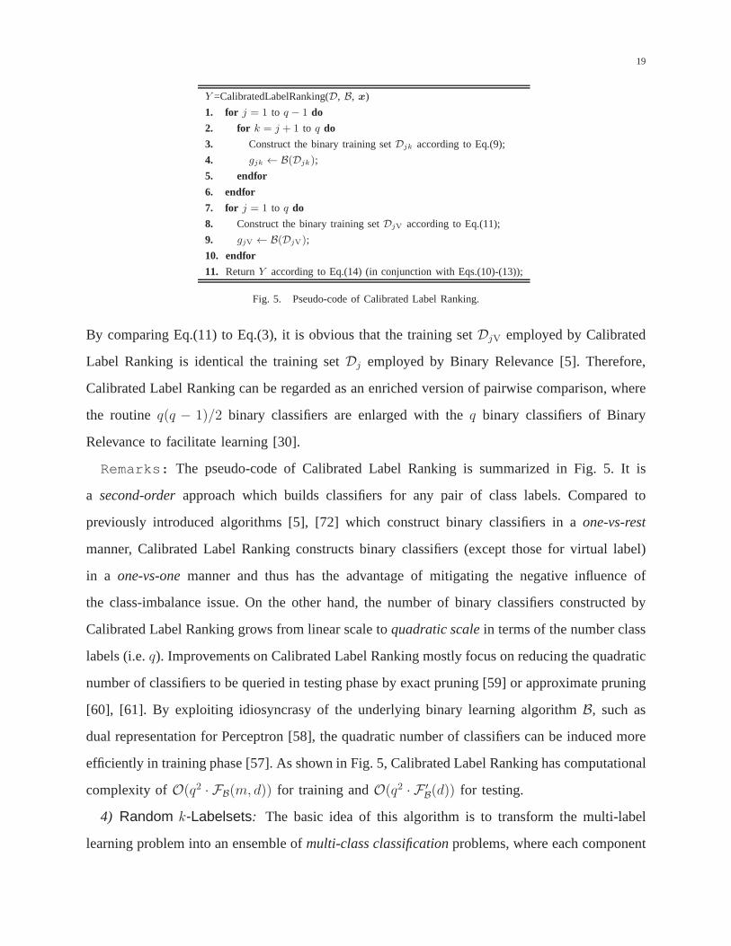
Fig. 5. Pseudo-code of Calibrated Label Ranking.

By comparing Eq.(11) to Eq.(3), it is obvious that the training set DjV employed by Calibrated

Label Ranking is identical the training set Dj employed by Binary Relevance [5]. Therefore,

Calibrated Label Ranking can be regarded as an enriched version of pairwise comparison, where

the routine q(q − 1)/2 binary classifiers are enlarged with the q binary classifiers of Binary

Relevance to facilitate learning [30].

Remarks: The pseudo-code of Calibrated Label Ranking is summarized in Fig. 5. It is

a second-order approach which builds classifiers for any pair of class labels. Compared to

previously introduced algorithms [5], [72] which construct binary classifiers in a one-vs-rest

manner, Calibrated Label Ranking constructs binary classifiers (except those for virtual label)

in a one-vs-one manner and thus has the advantage of mitigating the negative influence of

the class-imbalance issue. On the other hand, the number of binary classifiers constructed by

Calibrated Label Ranking grows from linear scale to quadratic scale in terms of the number class

labels (i.e. q). Improvements on Calibrated Label Ranking mostly focus on reducing the quadratic

number of classifiers to be queried in testing phase by exact pruning [59] or approximate pruning

[60], [61]. By exploiting idiosyncrasy of the underlying binary learning algorithm B, such as

dual representation for Perceptron [58], the quadratic number of classifiers can be induced more

efficiently in training phase [57]. As shown in Fig. 5, Calibrated Label Ranking has computational

complexity of O(q2 · FB(m, d)) for training and O(q2 · F ′B(d)) for testing.

4) Random k-Labelsets: The basic idea of this algorithm is to transform the multi-label

learning problem into an ensemble of multi-class classification problems, where each component

20

learner in the ensemble targets a random subset of Y upon which a multi-class classifier is induced

by the Label Powerset (LP) techniques [92], [94].

LP is a straightforward approach to transforming multi-label learning problem into multi-

class (single-label) classification problem. Let σY : 2Y → N be some injective function mapping

from the power set of Y to natural numbers, and σ−1Y be the corresponding inverse function. In

the training phase, LP firstly converts the original multi-label training set D into the following

multi-class training set by treating every distinct label set appearing in D as a new class:

D†Y = {(xi, σY(Yi)) | 1 ≤ i ≤ m} (15)

where the set of new classes covered by D†Y corresponds to:

Γ(

D†Y

)

= {σY(Yi) | 1 ≤ i ≤ m} (16)

Obviously,

∣

∣

∣Γ(

D†Y

)∣

∣

∣≤ min

(

m, 2|Y|)

holds here. After that, some multi-class learning algorithm

M is utilized to induce a multi-class classifier g†Y : X → Γ(

D†Y

)

, i.e. g†Y ← M(

D†Y

)

.

Therefore, for any multi-label training example (xi, Yi), instance xi will be re-assigned with the

newly mapped single-label σY(Yi) and then participates in multi-class classifier induction.

For unseen instance x, LP predicts its associated label set Y by firstly querying the prediction

of multi-class classifier and then mapping it back to the power set of Y :

Y = σ−1Y

(

g†Y(x))

(17)

Unfortunately, LP has two major limitations in terms of practical feasibility: a) Incompleteness:

as shown in Eqs.(16) and (17), LP is confined to predict label sets appearing in the training set,

i.e. unable to generalize to those outside {Yi | 1 ≤ i ≤ m}; b) Inefficiency: when Y is large,

there might be too many newly mapped classes in Γ(

D†Y

)

, leading to overly high complexity

in training g†Y(·) and extremely few training examples for some newly mapped classes.

To keep LP’s simplicity while overcoming its two major drawbacks, Random k-Labelsets

chooses to combine ensemble learning [24], [112] with LP to learn from multi-label data. The

key strategy is to invoke LP only on random k-labelsets (size-k subset in Y) to guarantee

computational efficiency, and then ensemble a number of LP classifiers to achieve predictive

completeness.

21

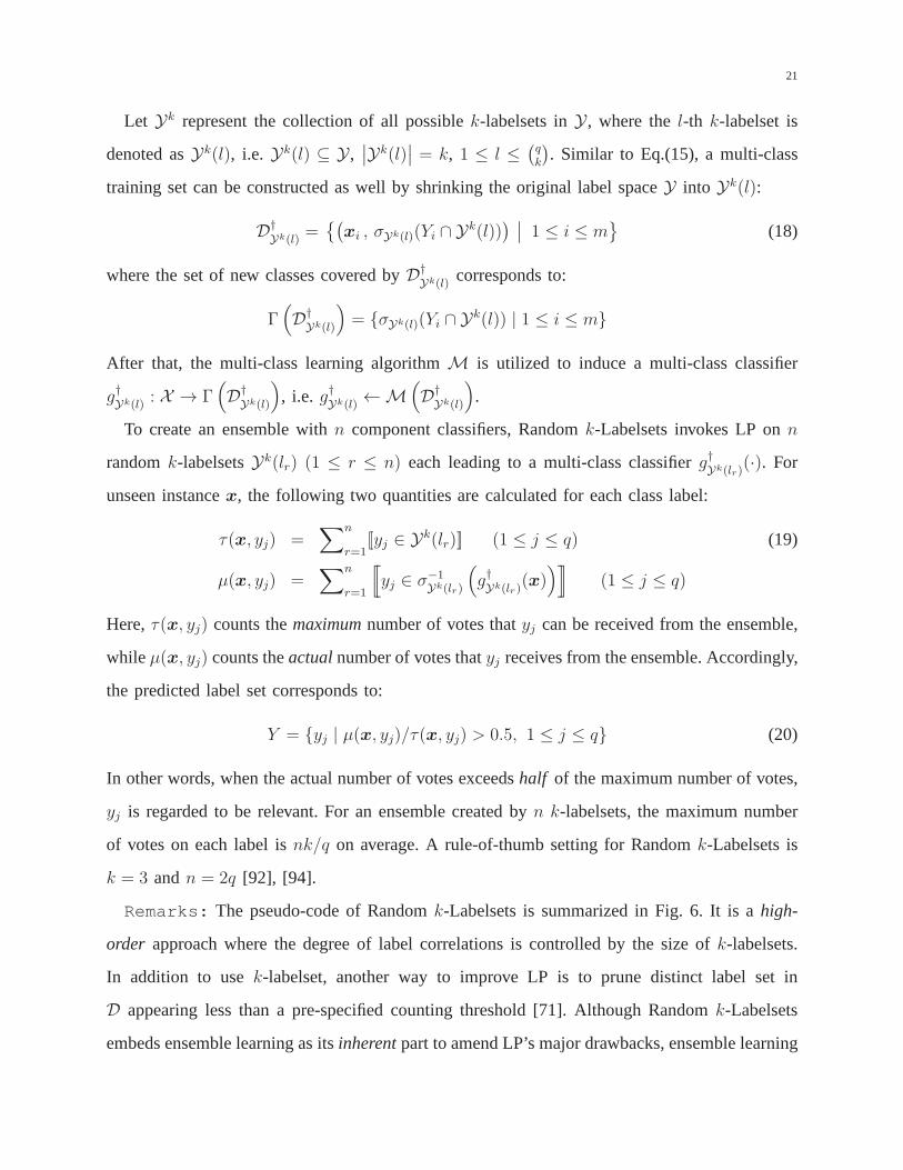
Let Yk represent the collection of all possible k-labelsets in Y , where the l-th k-labelset is

denoted as Yk(l), i.e. Yk(l) ⊆ Y ,∣

∣Yk(l)∣

∣ = k, 1 ≤ l ≤(

q

k

)

. Similar to Eq.(15), a multi-class

training set can be constructed as well by shrinking the original label space Y into Yk(l):

D†Yk(l)

={(

xi , σYk(l)(Yi ∩ Yk(l))

)∣

∣ 1 ≤ i ≤ m}

(18)

where the set of new classes covered by D†Yk(l)

corresponds to:

Γ(

D†Yk(l)

)

= {σYk(l)(Yi ∩ Yk(l)) | 1 ≤ i ≤ m}

After that, the multi-class learning algorithm M is utilized to induce a multi-class classifier

g†Yk(l)

: X → Γ(

D†Yk(l)

)

, i.e. g†Yk(l)←M

(

D†Yk(l)

)

.

To create an ensemble with n component classifiers, Random k-Labelsets invokes LP on n

random k-labelsets Yk(lr) (1 ≤ r ≤ n) each leading to a multi-class classifier g†Yk(lr)

(·). For

unseen instance x, the following two quantities are calculated for each class label:

τ(x, yj) =∑n

r=1[[yj ∈ Y

k(lr)]] (1 ≤ j ≤ q) (19)

µ(x, yj) =∑n

r=1

[[

yj ∈ σ−1Yk(lr)

(

g†Yk(lr)

(x))]]

(1 ≤ j ≤ q)

Here, τ(x, yj) counts the maximum number of votes that yj can be received from the ensemble,

while µ(x, yj) counts the actual number of votes that yj receives from the ensemble. Accordingly,

the predicted label set corresponds to:

Y = {yj | µ(x, yj)/τ(x, yj) > 0.5, 1 ≤ j ≤ q} (20)

In other words, when the actual number of votes exceeds half of the maximum number of votes,

yj is regarded to be relevant. For an ensemble created by n k-labelsets, the maximum number

of votes on each label is nk/q on average. A rule-of-thumb setting for Random k-Labelsets is

k = 3 and n = 2q [92], [94].

Remarks: The pseudo-code of Random k-Labelsets is summarized in Fig. 6. It is a high-

order approach where the degree of label correlations is controlled by the size of k-labelsets.

In addition to use k-labelset, another way to improve LP is to prune distinct label set in

D appearing less than a pre-specified counting threshold [71]. Although Random k-Labelsets

embeds ensemble learning as its inherent part to amend LP’s major drawbacks, ensemble learning

22

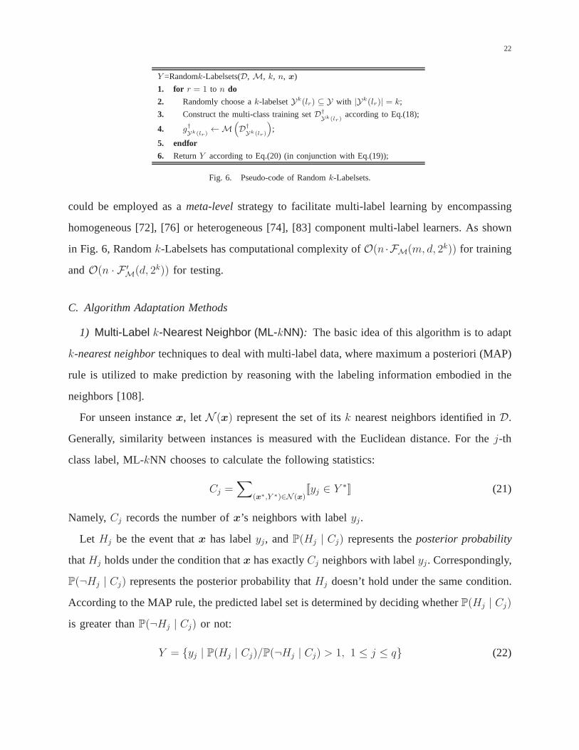
Y =Randomk-Labelsets(D, M, k, n, x)

1. for r = 1 to n do

2. Randomly choose a k-labelset Yk(lr) ⊆ Y with |Yk(lr)| = k;

3. Construct the multi-class training set D†

Yk(lr)according to Eq.(18);

4. g†Yk(lr)

←M(

D†

Yk(lr)

)

;

5. endfor

6. Return Y according to Eq.(20) (in conjunction with Eq.(19));

Fig. 6. Pseudo-code of Random k-Labelsets.

could be employed as a meta-level strategy to facilitate multi-label learning by encompassing

homogeneous [72], [76] or heterogeneous [74], [83] component multi-label learners. As shown

in Fig. 6, Random k-Labelsets has computational complexity of O(n ·FM(m, d, 2k)) for training

and O(n · F ′M(d, 2k)) for testing.

C. Algorithm Adaptation Methods

1) Multi-Label k-Nearest Neighbor (ML-kNN): The basic idea of this algorithm is to adapt

k-nearest neighbor techniques to deal with multi-label data, where maximum a posteriori (MAP)

rule is utilized to make prediction by reasoning with the labeling information embodied in the

neighbors [108].

For unseen instance x, let N (x) represent the set of its k nearest neighbors identified in D.

Generally, similarity between instances is measured with the Euclidean distance. For the j-th

class label, ML-kNN chooses to calculate the following statistics:

Cj =∑

(x∗,Y ∗)∈N (x)[[yj ∈ Y

∗]] (21)

Namely, Cj records the number of x’s neighbors with label yj .

Let Hj be the event that x has label yj , and P(Hj | Cj) represents the posterior probability

that Hj holds under the condition that x has exactly Cj neighbors with label yj . Correspondingly,

P(¬Hj | Cj) represents the posterior probability that Hj doesn’t hold under the same condition.

According to the MAP rule, the predicted label set is determined by deciding whether P(Hj | Cj)

is greater than P(¬Hj | Cj) or not:

Y = {yj | P(Hj | Cj)/P(¬Hj | Cj) > 1, 1 ≤ j ≤ q} (22)

23

Based on Bayes theorem, we have:

P(Hj | Cj)

P(¬Hj | Cj)=

P(Hj) · P(Cj | Hj)

P(¬Hj) · P(Cj | ¬Hj)(23)

Here, P(Hj) (P(¬Hj)) represents the prior probability that Hj holds (doesn’t hold). Furthermore,

P(Cj | Hj) (P(Cj | ¬Hj)) represents the likelihood that x has exactly Cj neighbors with label

yj when Hj holds (doesn’t hold). As shown in Eqs.(22) and (23), it suffices to estimate the prior

probabilities as well as likelihoods for making predictions.

ML-kNN fulfills the above task via the frequency counting strategy. Firstly, the prior proba-

bilities are estimated by counting the number training examples associated with each label:

P(Hj) =s+

∑m

i=1[[yj ∈ Yi]]

s× 2 +m; P(¬Hj) = 1− P(Hj) (1 ≤ j ≤ q) (24)

Here, s is a smoothing parameter controlling the effect of uniform prior on the estimation.

Generally, s takes the value of 1 resulting in Laplace smoothing.

Secondly, the estimation process for likelihoods is somewhat involved. For the j-th class label

yj , ML-kNN maintains two frequency arrays κj and κj each containing k+1 elements:

κj[r] =∑m

i=1[[yj ∈ Yi]] · [[δj(xi) = r]] (0 ≤ r ≤ k) (25)

κj[r] =∑m

i=1[[yj /∈ Yi]] · [[δj(xi) = r]] (0 ≤ r ≤ k)

where δj(xi) =∑

(x∗,Y ∗)∈N (xi)[[yj ∈ Y

∗]]

Here, δj(xi) records the number of xi’s neighbors with label yj . Therefore, κj [r] counts the

number of training examples which have label yj and have exactly r neighbors with label yj ,

while κj [r] counts the number of training examples which don’t have label yj and have exactly

r neighbors with label yj . Afterwards, the likelihoods can be estimated based on κj and κj :

P(Cj | Hj) =s+ κj [Cj]

s× (k + 1) +∑k

r=0 κj [r](1 ≤ j ≤ q, 0 ≤ Cj ≤ k) (26)

P(Cj | ¬Hj) =s+ κj [Cj]

s× (k + 1) +∑k

r=0 κj [r](1 ≤ j ≤ q, 0 ≤ Cj ≤ k)

Thereafter, by substituting Eq.(24) (prior probabilities) and Eq.(26) (likelihoods) into Eq.(23),

the predicted label set in Eq.(22) naturally follows.

24

Y =ML-kNN(D, k, x)

1. for i = 1 to m do

2. Identify k nearest neighbors N (xi) for xi;

3. endfor


5. Estimate the prior probabilities P(Hj) and P(¬Hj) according to Eq.(24);

6. Maintain frequency arrays κj and κj according to Eq.(25);

7. endfor

8. Identify k nearest neighbors N (x) for x;


10. Calculate statistic Cj according to Eq.(21);

11. endfor

12. Return Y according to Eq.(22) (in conjunction with Eqs.(23), (24) and (26));

Fig. 7. Pseudo-code of ML-kNN.

Remarks: The pseudo-code of ML-kNN is summarized in Fig. 7. It is a first-order approach

which reasons the relevance of each label separately. ML-kNN has the advantage of inheriting

merits of both lazy learning and Bayesian reasoning: a) decision boundary can be adaptively

adjusted due to the varying neighbors identified for each unseen instance; b) the class-imbalance

issue can be largely mitigated due to the prior probabilities estimated for each class label. There

are other ways to make use of lazy learning for handling multi-label data, such as combining

kNN with ranking aggregation [7], [15], identifying kNN in a label-specific style [41], [101],

expanding kNN to cover the whole training set [14], [49]. Considering that ML-kNN is ignorant

of exploiting label correlations, several extensions have been proposed to provide patches to

ML-kNN along this direction [13], [104]. As shown in Fig. 7, ML-kNN has computational

complexity of O(m2d+ qmk) for training and O(md+ qk) for testing.

2) Multi-Label Decision Tree (ML-DT): The basic idea of this algorithm is to adopt decision

tree techniques to deal with multi-label data, where an information gain criterion based on multi-

label entropy is utilized to build the decision tree recursively [16].

Given any multi-label data set T = {(xi, Yi) | 1 ≤ i ≤ n} with n examples, the information

gain achieved by dividing T along the l-th feature at splitting value ϑ is:

IG(T , l, ϑ) = MLEnt(T )−∑

ρ∈{−,+}

|T ρ|

|T |·MLEnt(T ρ) (27)

where T − = {(xi, Yi) | xil ≤ ϑ, 1 ≤ i ≤ n}, T + = {(xi, Yi) | xil > ϑ, 1 ≤ i ≤ n}

25

Namely, T − (T +) consists of examples with values on the l-th feature less (greater) than ϑ.9

Starting from the root node (i.e. T = D), ML-DT identifies the feature and the corresponding

splitting value which maximizes the information gain in Eq.(27), and then generates two child

nodes with respect to T − and T +. The above process is invoked recursively by treating either

T − or T + as the new root node, and terminates until some stopping criterion C is met (e.g. size

of the child node is less than the pre-specified threshold).

To instantiate ML-DT, the mechanism for computing multi-label entropy, i.e. MLEnt(·) in

Eq.(27), needs to be specified. A straightforward solution is to treat each subset Y ⊆ Y as a

new class and then resort to the conventional single-label entropy:

MLEnt(T ) = −∑

Y⊆YP(Y ) · log2(P(Y )) (28)

where P(Y ) =

∑n

i=1[[Yi = Y ]]

n

However, as the number of new classes grows exponentially with respect to |Y|, many of them

might not even appear in T and thus only have trivial estimated probability (i.e. P(Y ) = 0). To

circumvent this issue, ML-DT assumes independence among labels and computes the multi-label

entropy in a decomposable way:

MLEnt(T ) =∑q

j=1−pj log2 pj − (1− pj) log2(1− pj) (29)

where pj =

∑n

i=1[[yj ∈ Yi]]

n

Here, pj represents the fraction of examples in T with label yj . Note that Eq.(29) can be regarded

as a simplified version of Eq.(28) under the label independence assumption, and it holds that

MLEnt(T ) ≥ MLEnt(T ).

For unseen instance x, it is fed to the learned decision tree by traversing along the paths until

reaching a leaf node affiliated with a number of training examples T ⊆ D. Then, the predicted

label set corresponds to:

Y = {yj | pj > 0.5, 1 ≤ j ≤ q} (30)

9Without loss of generality, here we assume that features are real-valued and the data set is bi-partitioned by setting splitting

point along each feature. Similar to Eq.(27), information gain with respect to discrete-valued features can be defined as well.

26

Y =ML-DT(D, C, x)

1. Create a decision tree with root node N affiliated with the whole training set (T = D);

2. if stopping criterion C is met then

3. break and go to step 9;

4. else

5. Identify the feature-value pair (l, ϑ) which maximizes Eq.(27);

6. Set T − and T + according to Eq.(27);

7. Set N .lsubtree and N .rsubtree to the decision trees recursively constructed with T − and T + respectively;

8. endif

9. Traverse x along the decision tree from the root node until a leaf node is reached;


Fig. 8. Pseudo-code of ML-DT.

In other words, if for one leaf node the majority of training examples falling into it have label

yj , any test instance allocated within the same leaf node will regard yj as its relevant label.

Remarks: The pseudo-code of ML-DT is summarized in Fig. 8. It is a first-order approach

which assumes label independence in calculating multi-label entropy. One prominent advantage

of ML-DT lies in its high efficiency in inducing the decision tree model from multi-label data.

Possible improvements on multi-label decision trees include employing pruning strategy [16]

or ensemble learning techniques [52], [110]. As shown in Fig. 8, ML-DT has computational

complexity of O(mdq) for training and O(mq) for testing.

3) Ranking Support Vector Machine (Rank-SVM): The basic idea of this algorithm is to

adapt maximum margin strategy to deal with multi-label data, where a set of linear classifiers

are optimized to minimize the empirical ranking loss and enabled to handle nonlinear cases with

kernel tricks [27].

Let the learning system be composed of q linear classifiersW = {(wj, bj) | 1 ≤ j ≤ q}, where

wj ∈ Rd and bj ∈ R are the weight vector and bias for the j-th class label yj . Correspondingly,

Rank-SVM defines the learning system’s margin on (xi, Yi) by considering its ranking ability

on the example’s relevant and irrelevant labels:

min(yj ,yk)∈Yi×Yi

〈wj −wk,xi〉+ bj − bk‖wj −wk‖

(31)

Here, 〈u, v〉 returns the inner product u⊤v. Geometrically speaking, for each relevant-irrelevant

label pair (yj, yk) ∈ Yi× Yi, their discrimination boundary corresponds to the hyperplane 〈wj −

wk,x〉+ bj − bk = 0. Therefore, Eq.(31) considers the signed L2-distance of xi to hyperplanes

27

of every relevant-irrelevant label pair, and then returns the minimum as the margin on (xi, Yi).

Therefore, the learning system’s margin on the whole training set D naturally follows:

min(xi,Yi)∈D


〈wj −wk,xi〉+ bj − bk‖wj −wk‖

(32)

When the learning system is capable of properly ranking every relevant-irrelevant label pair for

each training example, Eq.(32) will return positive margin. In this ideal case, we can rescale the

linear classifiers to ensure: a) ∀ 1 ≤ i ≤ m and (yj, yk) ∈ Yi× Yi, 〈wj −wk,xi〉+ bj − bk > 1;

b) ∃ i∗ ∈ {1, · · · , m} and (yj∗, yk∗) ∈ Yi∗ × Yi∗ , 〈wj∗ −wk∗ ,xi∗〉 + bj∗ − bk∗ = 1. Thereafter,

the problem of maximizing the margin in Eq.(32) can be expressed as:

maxW

min(xi,Yi)∈D


1

‖wj −wk‖2(33)

subject to : 〈wj −wk,xi〉+ bj − bk ≥ 1 (1 ≤ i ≤ m, (yj, yk) ∈ Yi × Yi)

Suppose we have sufficient training examples such that for each label pair (yj, yk) (j 6= k), there

exists (x, Y ) ∈ D satisfying (yj, yk) ∈ Y × Y . Thus, the objective in Eq.(33) becomes equivalent

to maxW min1≤j<k≤q1

‖wj−wk‖2and the optimization problem can be re-written as:

minW

max1≤j<k≤q

‖wj −wk‖2 (34)


To overcome the difficulty brought by the max operator, Rank-SVM chooses to simplify Eq.(34)

by approximating the max operator with the sum operator:

minW

∑q

j=1‖wj‖

2 (35)


To accommodate real-world scenarios where constraints in Eq.(35) can not be fully satisfied,

slack variables can be incorporated into Eq.(35):

min{W ,Ξ}

∑q

j=1‖wj‖

2 + C∑m

i=1

1

|Yi||Yi|

∑

(yj ,yk)∈Yi×Yi

ξijk (36)

subject to : 〈wj −wk,xi〉+ bj − bk ≥ 1− ξijk

ξijk ≥ 0 (1 ≤ i ≤ m, (yj, yk) ∈ Yi × Yi)

28

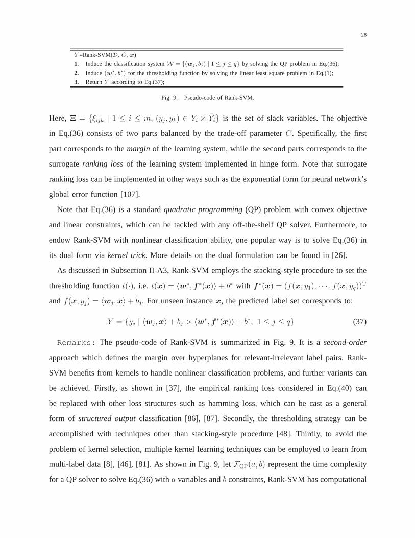
Y =Rank-SVM(D, C, x)

1. Induce the classification system W = {(wj , bj) | 1 ≤ j ≤ q} by solving the QP problem in Eq.(36);

2. Induce (w∗, b∗) for the thresholding function by solving the linear least square problem in Eq.(1);


Fig. 9. Pseudo-code of Rank-SVM.

Here, Ξ = {ξijk | 1 ≤ i ≤ m, (yj, yk) ∈ Yi × Yi} is the set of slack variables. The objective

in Eq.(36) consists of two parts balanced by the trade-off parameter C. Specifically, the first

part corresponds to the margin of the learning system, while the second parts corresponds to the

surrogate ranking loss of the learning system implemented in hinge form. Note that surrogate

ranking loss can be implemented in other ways such as the exponential form for neural network’s

global error function [107].

Note that Eq.(36) is a standard quadratic programming (QP) problem with convex objective

and linear constraints, which can be tackled with any off-the-shelf QP solver. Furthermore, to

endow Rank-SVM with nonlinear classification ability, one popular way is to solve Eq.(36) in

its dual form via kernel trick. More details on the dual formulation can be found in [26].

As discussed in Subsection II-A3, Rank-SVM employs the stacking-style procedure to set the

thresholding function t(·), i.e. t(x) = 〈w∗, f ∗(x)〉+ b∗ with f ∗(x) = (f(x, y1), · · · , f(x, yq))T

and f(x, yj) = 〈wj,x〉+ bj . For unseen instance x, the predicted label set corresponds to:

Y = {yj | 〈wj,x〉+ bj > 〈w∗, f ∗(x)〉+ b∗, 1 ≤ j ≤ q} (37)

Remarks: The pseudo-code of Rank-SVM is summarized in Fig. 9. It is a second-order

approach which defines the margin over hyperplanes for relevant-irrelevant label pairs. Rank-

SVM benefits from kernels to handle nonlinear classification problems, and further variants can

be achieved. Firstly, as shown in [37], the empirical ranking loss considered in Eq.(40) can

be replaced with other loss structures such as hamming loss, which can be cast as a general

form of structured output classification [86], [87]. Secondly, the thresholding strategy can be

accomplished with techniques other than stacking-style procedure [48]. Thirdly, to avoid the

problem of kernel selection, multiple kernel learning techniques can be employed to learn from

multi-label data [8], [46], [81]. As shown in Fig. 9, let FQP(a, b) represent the time complexity

for a QP solver to solve Eq.(36) with a variables and b constraints, Rank-SVM has computational

29

complexity of O(FQP(dq +mq2, mq2) + q2(q +m)) for training and O(dq) for testing.

4) Collective Multi-Label Classifier (CML): The basic idea of this algorithm is to adapt

maximum entropy principle to deal with multi-label data, where correlations among labels are

encoded as constraints that the resulting distribution must satisfy [33].

For any multi-label example (x, Y ), let (x,y) be the corresponding random variables repre-

sentation using binary label vector y = (y1, y2, · · · , yq)⊤ ∈ {−1,+1}q, whose j-th component

indicates whether Y contains the j-th label (yj = +1) or not (yj = −1). Statistically speaking,

the task of multi-label learning is equivalent to learn a joint probability distribution p(x,y).

Let Hp(x,y) represent the information entropy of (x,y) given their distribution p(·, ·). The

principle of maximum entropy [45] assumes that the distribution best modeling the current state

of knowledge is the one maximizing Hp(x,y) subject to a collection K of given facts:

maxpHp(x,y) (38)

subject to : Ep[fk(x,y)] = Fk (k ∈ K)

Generally, the fact is expressed as constraint on the expectation of some function over (x,y),

i.e. by imposing Ep[fk(x,y)] = Fk. Here, Ep[·] is the expectation operator with respect to p(·, ·),

while Fk corresponds to the expected value estimated from training set, e.g. 1m

∑

(x,y)∈D fk(x,y).

Together with the normalization constraint on p(·, ·) (i.e. Ep[1] = 1), the constrained opti-

mization problem of Eq.(38) can be carried out with standard Lagrange Multiplier techniques.

Accordingly, the optimal solution is shown to fall within the Gibbs distribution family [1]:

p(y | x) =1

ZΛ(x)exp

(

∑

k∈Kλk · fk(x,y)

)

(39)

Here, Λ = {λk | k ∈ K} is the set of parameters to be determined, and ZΛ(x) is the partition

function serving as the normalization factor, i.e. ZΛ(x) =∑

yexp

(∑

k∈K λk · fk(x,y))

.

By assuming Gaussian prior (i.e. λk ∼ N (0, ε2)), parameters in Λ can be found by maximizing

the following log-posterior probability function:

l(Λ | D) = log

(

∏

(x,y)∈Dp(y | x)

)

−∑

k∈K

λ2k2ε2

(40)

=∑

(x,y)∈D

(

∑

k∈Kλk · fk(x,y)− logZΛ(x)

)

−∑

k∈K

λ2k2ε2

30

Y =CML(D, ε2, x)

1. for l = 1 to d do


3. Set constraint fk(x,y) = xl · [[yj = 1]] (k = (l, j) ∈ K1);

4. endfor

5. endfor

6. for j1 = 1 to q − 1 do

7. for j2 = j1 + 1 to q do

8. Set constraint fk(x,y) = [[yj1 = b1]] · [[yj2 = b2]] (b1, b2 ∈ {−1,+1}, k = (j1, j2, b1, b2) ∈ K2);

9. endfor

10. endfor

11. Determine parameters Λ = {λk | k ∈ K1

⋃

K2} by maximizing Eq.(40) (in conjunction with Eq.(41));


Fig. 10. Pseudo-code of CML.

Note that Eq.(40) is a convex function over Λ, whose global maximum (though not in closed-

form) can be found by any off-the-shelf unconstrained optimization method such as BFGS [9].

Generally, gradients of l(Λ | D) are needed by most numerical methods:

∂l(Λ | D)

∂λk=∑

(x,y)∈D

(

fk(x,y)−∑

y

fk(x,y)p(y | x))

−λkε2

(k ∈ K) (41)

For CML, the set of constraints consists of two parts K = K1

⋃

K2. Concretely, K1 = {(l, j) |

1 ≤ l ≤ d, 1 ≤ j ≤ q} specifies a total of d · q constraints with fk(x,y) = xl · [[yj = 1]] (k =

(l, j) ∈ K1). In addition, K2 = {(j1, j2, b1, b2) | 1 ≤ j1 < j2 ≤ q, b1, b2 ∈ {−1,+1}} specifies

a total of 4 ·(

q

2

)

constraints with fk(x,y) = [[yj1 = b1]] · [[yj2 = b2]] (k = (j1, j2, b1, b2) ∈ K2).

Actually, constraints in K can be specified in other ways yielding variants of CML [33], [114].

For unseen instance x, the predicted label set corresponds to:

Y = argmaxy

p(y | x) (42)

Note that exact inference with argmax is only tractable for small label space. Otherwise, pruning

strategies need to be applied to significantly reduce the search space of argmax, e.g. only

considering label sets appearing in the training set [33].

Remarks: The pseudo-code of CML is summarized in Fig. 10. It is a second-order approach

where correlations between every label pair are considered via constraints in K2. The second-

order correlation studied by CML is more general than that of Rank-SVM [27] as the latter only

considers relevant-irrelevant label pairs. As a conditional random field (CRF) model, CML is

31

TABLE II

SUMMARY OF REPRESENTATIVE MULTI-LABEL LEARNING ALGORITHMS BEING REVIEWED.

Order of Complexity Tested

Algorithm Basic Idea Correlations [Train/Test] Domains Optimized Metric

Binary Fit multi-label data to O(q · FB(m,d))/ classification

Relevance [5] q binary classifiers first-order O(q · F ′B(d)) image (hamming loss)

Classifier Fit multi-label data to a O(q · FB(m,d+ q))/ image, video classification

Chains [72] chain of binary classifiers high-order O(q · F ′B(d+ q)) text, biology (hamming loss)

Calibrated Label Fit multi-label data to O(q2 · FB(m, d))/ image, text Ranking

Ranking [30]q(q+1)

2binary classifiers second-order O(q2 · F ′

B(d)) biology (ranking loss)

Random Fit multi-label data to O(n · FM(m, d, 2k))/ image, text classification

k-Labelsets [94] n multi-class classifiers high-order O(n · F ′M(d, 2k)) biology (subset accuracy)

Fit k-nearest neighbor O(m2d+ qmk)/ image, text classification

ML-kNN [108] to multi-label data first-order O(md+ qk) biology (hamming loss)

Fit decision tree classification

ML-DT [16] to multi-label data first-order O(mdq)/O(mq) biology (hamming loss)

Fit kernel learning O(FQP(dq +mq2,mq2) Ranking

Rank-SVM [27] to multi-label data second-order +q2(q +m))/O(dq) biology (ranking loss)

Fit conditional random O(FUNC(dq + q2,m))/ classification

CML [33] field to multi-label data second-order O((dq + q2) · 2q) text (subset accuracy)

interested in using the conditional probability distribution p(y | x) in Eq.(39) for classification.

Interestingly, p(y | x) can be factored in various ways such as p(y | x) =∏q

j=1 p(yj |

x, y1, · · · , yj−1) where each term in the product can be modeled by one classifier in the classifier

chain [20], [72], or p(y | x) =∏q

j=1 p(yj | x,paj) where each term in the product can be

modeled by node yj and its parents paj in a directed graph [36], [105], [106], and efficient

algorithms exist when the directed graph corresponds to multi-dimensional Bayesian network

with restricted topology [4], [18], [98]. Directed graphs are also found to be useful for modeling

multiple fault diagnosis where yj indicates the good/failing condition of one of the device’s

components [3], [19]. On the other hand, there have been some multi-label generative models

which aim to model the joint probability distribution p(x,y) [63], [80], [97]. As shown in Fig.

10, let FUNC(a,m) represent the time complexity for an unconstrained optimization method to

solve Eq.(40) with a variables, CML has computational complexity of O(FUNC(dq+ q2, m)) for

training and O((dq + q2) · 2q) for testing.

32

D. Summary

Table II summarizes properties of the eight multi-label learning algorithms investigated in Sub-

sections III-B and III-C, including their basic idea, label correlations, computational complexity,

tested domains, and optimized (surrogate) metric. As shown in Table II, (surrogate) hamming loss

and ranking loss are among the most popular metrics to be optimized and theoretical analyses on

them [21]–[23], [32] have been discussed in Subsection II-B4. Furthermore, note that the subset

accuracy optimized by Random k-Labelsets is only measured with respect to the k-labelset

instead of the whole label space.

Domains reported in Table II correspond to data types on which the corresponding algorithm

is shown to work well in the original literature. However, all those representative multi-label

learning algorithms are general-purpose and can be applied to various data types. Nevertheless,

the computational complexity of each learning algorithm does play a key factor on its suitability

for different scales of data. Here, the data scalability can be studied in terms of three main

aspects including the number of training examples (i.e. m), the dimensionality (i.e. d), and the

number of possible class labels (i.e. q). Furthermore, algorithms which append class labels as

extra features to instance space [20], [72], [106] might not benefit too much from this strategy

when instance dimensionality is much larger than the number of class labels (i.e. d≫ q).

As arguably the mostly-studied supervised learning framework, several algorithms in Table

II employ binary classification as the intermediate step to learn from multi-label data [5], [30],

[72]. An initial and general attempt towards binary classification transformation comes from

the famous AdaBoost.MH algorithm [75], where each multi-label training example (xi, Yi) is

converted into q binary examples {([xi, yj] , φ(Yi, yj)) | 1 ≤ j ≤ q}. It can be regarded as a high-

order approach where labels in Y are treated as appending feature to X and would be related

to each other via the shared instance x, as far as the binary learning algorithm B is capable of

capturing dependencies among features. Other ways towards binary classification transformation

can be fulfilled with techniques such as stacked aggregation [34], [64], [88] or Error-Correcting

Output Codes (ECOC) [28], [111].

In addition, first-order algorithm adaptation methods can not be simply regarded as Binary

33

Relevance [5] combined with specific binary learners. For example, ML-kNN [108] is more than

Binary Relevance combined with kNN as Bayesian inference is employed to reason with neigh-

boring information, and ML-DT [16] is more than Binary Relevance combined with decision

tree as a single decision tree instead of q decision trees is built to accommodate all class labels

(based on multi-label entropy).

IV. RELATED LEARNING SETTINGS

There are several learning settings related to multi-label learning which are worth some

discussion, such as multi-instance learning [25], ordinal classification [29], multi-task learning

[10], and data streams classification [31].

Multi-instance learning [25] studies the problem where each example is described by a bag

of instances while associated with a single (binary) label. A bag is regarded to be positive iff

at least one of its constituent instances is positive. In contrast to multi-label learning which

models the object’s ambiguities (complicated semantics) in output (label) space, multi-instance

learning can be viewed as modeling the object’s ambiguities in input (instance) space [113].

There are some initial attempt towards exploiting multi-instance representation for learning from

multi-label data [109].

Ordinal classification [29] studies the problem where a natural ordering exists among all

the class labels. In multi-label learning, we can accordingly assume an ordering of relevance on

each class label to generalize the crisp membership (yj ∈ {−1,+1}) into the graded membership

(yj ∈ {m1, m2, · · · , mk} where m1 < m2 < · · · < mk). Therefore, graded multi-label learning

accommodates the case where we can only provide vague (ordinal) instead of definite judgement

on the label relevance. Existing work shows that graded multi-label learning can be solved by

transforming it into a set of ordinal classification problems (one for each class label), or a set

of standard multi-label learning problems (one for each membership level) [12].

Multi-task learning [10] studies the problem where multiple tasks are trained in parallel such

that training information of related tasks are used as an inductive bias to help improve the

generalization performance of other tasks. Nonetheless, there are some essential differences

between multi-task learning and multi-label learning to be noticed. Firstly, in multi-label learning

34

all the examples share the same feature space, while in multi-task learning the tasks can be in

the same feature space or different feature spaces. Secondly, in multi-label learning the goal is

to predict the label subset associated with an object, while the purpose of multi-task learning

is to have multiple tasks to be learned well simultaneously, and it does not concern on which

task subset should be associated with an object (if we take a label as a task) since it generally

assumes that every object is involved by all tasks. Thirdly, in multi-label learning it is not

rare (yet demanding) to deal with large label space [90], while in multi-task learning it is not

reasonable to consider a large number of tasks. Nevertheless, techniques for multi-task learning

might be used to benefit multi-label learning [56].

Data streams classification [31] studies the problem where real-world objects are generated

online and processed in a real-time manner. Nowadays, streaming data with multi-label nature

widely exist in real-world scenarios such as instant news, emails, microblogs, etc [70]. As a

usual challenge for streaming data analysis, the key factor for effectively classifying multi-label

data streams is how to deal with the concept drift problem. Existing works model concept drift

by updating the classifiers significantly whenever a new batch of examples arrive [68], taking

the fading assumption that the influence of past data gradually declines as time evolves [53],

[78], or maintaining a change detector alerting whenever a concept drift is detected [70].

V. CONCLUSION

In this paper, the state-of-the-art of multi-label learning is reviewed in terms of paradigm

formalization, learning algorithms and related learning settings. In particular, instead of trying to

go through all the learning techniques within confined space, which would lead to only abridged

introductions, we choose to elaborate the algorithmic details of eight representative multi-label

learning algorithms with references to other related works. Some online resources for multi-label

learning are summarized in Table III, including academic activities (tutorial, workshops, special

issue), publicly-available software and data sets.

As discussed in Section II-A2, although the idea of exploiting label correlations have been

employed by various multi-label learning techniques, there has not been any formal characteri-

zation on the underlying concept or any principled mechanism on the appropriate usage of label

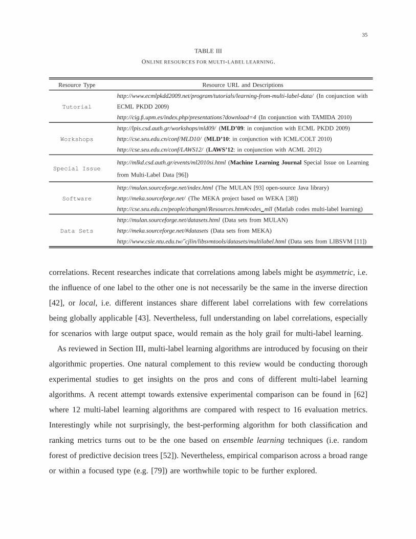
35

TABLE III

ONLINE RESOURCES FOR MULTI-LABEL LEARNING.

Resource Type Resource URL and Descriptions

http://www.ecmlpkdd2009.net/program/tutorials/learning-from-multi-label-data/ (In conjunction with

Tutorial ECML PKDD 2009)

http://cig.fi.upm.es/index.php/presentations?download=4 (In conjunction with TAMIDA 2010)

http://lpis.csd.auth.gr/workshops/mld09/ (MLD’09: in conjunction with ECML PKDD 2009)

Workshops http://cse.seu.edu.cn/conf/MLD10/ (MLD’10: in conjunction with ICML/COLT 2010)

http://cse.seu.edu.cn/conf/LAWS12/ (LAWS’12: in conjunction with ACML 2012)

Special Issuehttp://mlkd.csd.auth.gr/events/ml2010si.html (Machine Learning Journal Special Issue on Learning

from Multi-Label Data [96])

http://mulan.sourceforge.net/index.html (The MULAN [93] open-source Java library)

Software http://meka.sourceforge.net/ (The MEKA project based on WEKA [38])

http://cse.seu.edu.cn/people/zhangml/Resources.htm#codes mll (Matlab codes multi-label learning)

http://mulan.sourceforge.net/datasets.html (Data sets from MULAN)

Data Sets http://meka.sourceforge.net/#datasets (Data sets from MEKA)

http://www.csie.ntu.edu.tw/˜cjlin/libsvmtools/datasets/multilabel.html (Data sets from LIBSVM [11])

correlations. Recent researches indicate that correlations among labels might be asymmetric, i.e.

the influence of one label to the other one is not necessarily be the same in the inverse direction

[42], or local, i.e. different instances share different label correlations with few correlations

being globally applicable [43]. Nevertheless, full understanding on label correlations, especially

for scenarios with large output space, would remain as the holy grail for multi-label learning.

As reviewed in Section III, multi-label learning algorithms are introduced by focusing on their

algorithmic properties. One natural complement to this review would be conducting thorough

experimental studies to get insights on the pros and cons of different multi-label learning

algorithms. A recent attempt towards extensive experimental comparison can be found in [62]

where 12 multi-label learning algorithms are compared with respect to 16 evaluation metrics.

Interestingly while not surprisingly, the best-performing algorithm for both classification and

ranking metrics turns out to be the one based on ensemble learning techniques (i.e. random

forest of predictive decision trees [52]). Nevertheless, empirical comparison across a broad range

or within a focused type (e.g. [79]) are worthwhile topic to be further explored.

36

REFERENCES

[1] A. L. Berger, V. J. Della Pietra, and S. A. Della Pietra, “A maximum entropy approach to natural language processing,”

Computational Linguistics, vol. 22, no. 1, pp. 39–71, 1996.

[2] W. Bi and J. T. Kwok, “Multi-label classification on tree- and DAG-structured hierarchies,” in Proceedings of the 28th

International Conference on Machine Learning, Bellevue, WA, 2011, pp. 17–24.

[3] C. Bielza, G. Li, and P. Larranaga, “Multi-dimensional classification with Bayesian networks,” International Journal of

Approximate Reasoning, vol. 52, no. 6, pp. 705–727, 2011.

[4] H. Borchani, C. Bielza, C. Toro, and P. Larranaga, “Predicting human immunodeficiency virus type 1 inhibitors using

multi-dimensional Bayesian network classifiers,” Artificial Intelligence in Medicine, in press.

[5] M. R. Boutell, J. Luo, X. Shen, and C. M. Brown, “Learning multi-label scene classification,” Pattern Recognition, vol. 37,

no. 9, pp. 1757–1771, 2004.

[6] K. Brinker, J. Furnkranz, and E. Hullermeier, “A unified model for multilabel classification and ranking,” in Proceedings

of the 17th European Conference on Artificial Intelligence, Riva del Garda, Italy, 2006, pp. 489–493.

[7] K. Brinker and E. Hullermeier, “Case-based multilabel ranking,” in Proceedings of the 20th International Joint Conference

on Artificial Intelligence, Hyderabad, India, 2007, pp. 702–707.

[8] S. S. Bucak, R. Jin, and A. K. Jain, “Multi-label multiple kernel learning by stochastic approximation: Application to

visual object recognition,” in Advances in Neural Information Processing Systems 23, J. Lafferty, C. K. I. Williams,

J. Shawe-Taylor, R. S. Zemel, and A. Culotta, Eds. Cambridge, MA: MIT Press, 2010, pp. 325–333.

[9] R. H. Byrd, J. Nocedal, and R. B. Schnabel, “Representations of quasi-newton matrices and their use in limited memory

methods,” Mathematical Programming, vol. 63, no. 1-3, pp. 129–156, 1994.

[10] R. Caruana, “Multitask learning,” Machine Learning, vol. 28, no. 1, pp. 41–75, 1997.

[11] C.-C. Chang and C.-J. Lin, “LIBSVM: A library for support vector machines,” ACM Transactions on Intelligent Systems

and Technology, vol. 2, no. 3, 2011, Article 27, Software available at http://www.csie.ntu.edu.tw/˜cjlin/libsvm.

[12] W. Cheng, K. Dembczynski, and E. Hullermeier, “Graded multilabel classification: The ordinal case,” in Proceedings of

the 27th International Conference on Machine Learning, Haifa, Israel, 2010, pp. 223–230.

[13] W. Cheng and E. Hullermeier, “Combining instance-based learning and logistic regression for multilabel classification,”

Machine Learning, vol. 76, no. 2-3, pp. 211–225, 2009.

[14] ——, “A simple instance-based approach to multilabel classification using the Mallows model,” in Working Notes of the

First International Workshop on Learning from Multi-Label Data, Bled, Slovenia, 2009, pp. 28–38.

[15] T.-H. Chiang, H.-Y. Lo, and S.-D. Lin, “A ranking-based KNN approach for multi-label classification,” in Proceedings

of the 4th Asian Conference on Machine Learning, Singapore, 2012, pp. 81–96.

[16] A. Clare and R. D. King, “Knowledge discovery in multi-label phenotype data,” in Lecture Notes in Computer Science

2168, L. De Raedt and A. Siebes, Eds. Berlin: Springer, 2001, pp. 42–53.

[17] A. de Carvalho and A. A. Freitas, “A tutorial on multi-label classification techniques,” in Studies in Computational

Intelligence 205, A. Abraham, A. E. Hassanien, and V. Snasel, Eds. Berlin: Springer, 2009, pp. 177–195.

[18] P. R. de Waal and L. C. van der Gaag, “Inference and learning in multi-dimensional Bayesian network classifiers,” in

Lecture Notes in Artificial Intelligence 4724, K. Mellouli, Ed. Berlin: Springer, 2007, pp. 501–511.

[19] V. Delcroix, M.-A. Maalej, and S. Piechowiak, “Bayesian networks versus other probabilistic models for the multiple

diagnosis of large devices,” International Journal on Artificial Intelligence Tools, vol. 16, no. 3, pp. 417–433, 2007.

37

[20] K. Dembczynski, W. Cheng, and E. Hullermeier, “Bayes optimal multilabel classification via probabilistic classifier

chains,” in Proceedings of the 27th International Conference on Machine Learning, Haifa, Israel, 2010, pp. 279–286.

[21] K. Dembczynski, W. Kotłowski, and E. Hullermeier, “Consistent multilabel ranking through univariate loss minization,”

in Proceedings of the 29th International Conference on Machine Learning, Edinburgh, UK, 2012, pp. 1319–1326.

[22] K. Dembczynski, W. Waegeman, W. Cheng, and E. Hullermeier, “Regret analysis for performance metrics in multi-label

classification: The case of hamming loss and subset zero-one loss,” in Lecture Notes in Artificial Intelligence 6321,

J. Balcazar, F. Bonchi, A. Gionis, and M. Sebag, Eds. Berlin: Springer, 2010, pp. 280–295.

[23] ——, “On label dependence and loss minimization in multi-label classification,” Machine Learning, vol. 88, no. 1-2, pp.

5–45, 2012.

[24] T. G. Dietterich, “Ensemble methods in machine learning,” in Proceedings of the 1st International Workshop on Multiple

Classifier Systems, Cagliari, Italy, 2000, pp. 1–15.

[25] T. G. Dietterich, R. H. Lathrop, and T. Lozano-Perez, “Solving the multiple-instance problem with axis-parallel rectangles,”

Artificial Intelligence, vol. 89, no. 1-2, pp. 31–71, 1997.

[26] A. Elisseeff and J. Weston, “Kernel methods for multi-labelled classification and categorical regression problems,” BIOwulf

Technologies, Tech. Rep., 2001.

[27] ——, “A kernel method for multi-labelled classification,” in Advances in Neural Information Processing Systems 14,

T. G. Dietterich, S. Becker, and Z. Ghahramani, Eds. Cambridge, MA: MIT Press, 2002, pp. 681–687.

[28] C. S. Ferng and H. T. Lin, “Multi-label classification with error-correcting codes,” in Proceedings of the 3rd Asian

Conference on Machine Learning, Taoyuan, Taiwan, 2011, pp. 281–295.

[29] E. Frank and M. Hall, “A simple approach to ordinal classification,” in Lecture Notes in Computer Science 2167, L. De

Raedt and P. Flach, Eds. Berlin: Springer, 2001, pp. 145–156.

[30] J. Furnkranz, E. Hullermeier, E. Loza Mencıa, and K. Brinker, “Multilabel classification via calibrated label ranking,”

Machine Learning, vol. 73, no. 2, pp. 133–153, 2008.

[31] M. M. Gaber, A. Zaslavsky, and S. Krishnaswamy, “A survey of classification methods in data streams,” in Data Streams:

Models and Algorithms, C. C. Aggarwal, Ed. Berlin: Springer, 2007, pp. 39–59.

[32] W. Gao and Z.-H. Zhou, “On the consistency of multi-label learning,” in Proceedings of the 24th Annual Conference on

Learning Theory, Budapest, Hungary, 2011, pp. 341–358.

[33] N. Ghamrawi and A. McCallum, “Collective multi-label classification,” in Proceedings of the 14th ACM International

Conference on Information and Knowledge Management, Bremen, Germany, 2005, pp. 195–200.

[34] S. Godbole and S. Sarawagi, “Discriminative methods for multi-labeled classification,” in Lecture Notes in Artificial

Intelligence 3056, H. Dai, R. Srikant, and C. Zhang, Eds. Berlin: Springer, 2004, pp. 22–30.

[35] S. Gopal and Y. Yang, “Multilabel classification with meta-level features,” in Proceedings of the 33rd Annual International

ACM SIGIR Conference on Research and Development in Information Retrieval, Geneva, Switzerland, 2010, pp. 315–322.

[36] Y. Guo and S. Gu, “Multi-label classification using conditional dependency networks,” in Proceedings of the 22nd

International Joint Conference on Artificial Intelligence, Barcelona, Spain, 2011, pp. 1300–1305.

[37] Y. Guo and D. Schuurmans, “Adaptive large margin training for multilabel classification,” in Proceedings of the 25th

AAAI Conference on Artificial Intelligence, San Francisco, CA, 2011, pp. 374–379.

[38] M. Hall, E. Frank, G. Holmes, B. Pfahringer, P. Reutemann, and I. H. Witten, “The WEKA data mining software: An

update,” SIGKDD Explorations, vol. 11, no. 1, pp. 10–18, 2009.

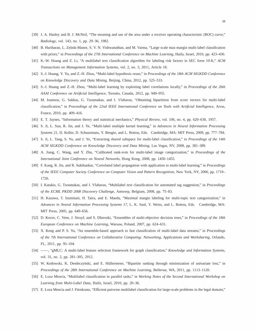
38

[39] J. A. Hanley and B. J. McNeil, “The meaning and use of the area under a receiver operating characteristic (ROC) curve,”

Radiology, vol. 143, no. 1, pp. 29–36, 1982.

[40] B. Hariharan, L. Zelnik-Manor, S. V. N. Vishwanathan, and M. Varma, “Large scale max-margin multi-label classification

with priors,” in Proceedings of the 27th International Conference on Machine Learning, Haifa, Israel, 2010, pp. 423–430.

[41] K.-W. Huang and Z. Li, “A multilabel text classification algorithm for labeling risk factors in SEC form 10-K,” ACM

Transactions on Management Information Systems, vol. 2, no. 3, 2011, Article 18.

[42] S.-J. Huang, Y. Yu, and Z.-H. Zhou, “Multi-label hypothesis reuse,” in Proceedings of the 18th ACM SIGKDD Conference

on Knowledge Discovery and Data Mining, Beijing, China, 2012, pp. 525–533.

[43] S.-J. Huang and Z.-H. Zhou, “Multi-label learning by exploiting label correlations locally,” in Proceedings of the 26th

AAAI Conference on Artificial Intelligence, Toronto, Canada, 2012, pp. 949–955.

[44] M. Ioannou, G. Sakkas, G. Tsoumakas, and I. Vlahavas, “Obtaining bipartition from score vectors for multi-label

classification,” in Proceedings of the 22nd IEEE International Conference on Tools with Artificial Intelligence, Arras,

France, 2010, pp. 409–416.

[45] E. T. Jaynes, “Information theory and statistical mechanics,” Physical Review, vol. 106, no. 4, pp. 620–630, 1957.

[46] S. Ji, L. Sun, R. Jin, and J. Ye, “Multi-label multiple kernel learning,” in Advances in Neural Information Processing

Systems 21, D. Koller, D. Schuurmans, Y. Bengio, and L. Bottou, Eds. Cambridge, MA: MIT Press, 2009, pp. 777–784.

[47] S. Ji, L. Tang, S. Yu, and J. Ye, “Extracting shared subspace for multi-label classification,” in Proceedings of the 14th

ACM SIGKDD Conference on Knowledge Discovery and Data Mining, Las Vegas, NV, 2008, pp. 381–389.

[48] A. Jiang, C. Wang, and Y. Zhu, “Calibrated rank-svm for multi-label image categorization,” in Proceedings of the

International Joint Conference on Neural Networks, Hong Kong, 2008, pp. 1450–1455.

[49] F. Kang, R. Jin, and R. Sukthankar, “Correlated label propagation with application to multi-label learning,” in Proceedings

of the IEEE Computer Society Conference on Computer Vision and Pattern Recognition, New York, NY, 2006, pp. 1719–

1726.

[50] I. Katakis, G. Tsoumakas, and I. Vlahavas, “Multilabel text classification for automated tag suggestion,” in Proceedings

of the ECML PKDD 2008 Discovery Challenge, Antwerp, Belgium, 2008, pp. 75–83.

[51] H. Kazawa, T. Izumitani, H. Taira, and E. Maeda, “Maximal margin labeling for multi-topic text categorization,” in

Advances in Neural Information Processing Systems 17, L. K. Saul, Y. Weiss, and L. Bottou, Eds. Cambridge, MA:

MIT Press, 2005, pp. 649–656.

[52] D. Kocev, C. Vens, J. Struyf, and S. Dzeroski, “Ensembles of multi-objective decision trees,” in Proceedings of the 18th

European Conference on Machine Learning, Warsaw, Poland, 2007, pp. 624–631.

[53] X. Kong and P. S. Yu, “An ensemble-based approach to fast classification of multi-label data streams,” in Proceedings

of the 7th International Conference on Collaborative Computing: Networking, Applications and Worksharing, Orlando,

FL, 2011, pp. 95–104.

[54] ——, “gMLC: A multi-label feature selection framework for graph classification,” Knowledge and Information Systems,

vol. 31, no. 2, pp. 281–305, 2012.

[55] W. Kotłowski, K. Dembczynski, and E. Hullermeier, “Bipartite ranking through minimization of univariate loss,” in

Proceedings of the 28th International Conference on Machine Learning, Bellevue, WA, 2011, pp. 1113–1120.

[56] E. Loza Mencıa, “Multilabel classification in parallel tasks,” in Working Notes of the Second International Workshop on

Learning from Multi-Label Data, Haifa, Israel, 2010, pp. 20–36.

[57] E. Loza Mencıa and J. Furnkranz, “Efficient pairwise multilabel classification for large-scale problems in the legal domain,”

39

in Lecture Notes in Artificial Intelligence 5212, W. Daelemans, B. Goethals, and K. Morik, Eds. Berlin: Springer, 2008,

pp. 50–65.

[58] ——, “Pairwise learning of multilabel classifications with perceptrons,” in Proceedings of the International Joint

Conference on Neural Networks, Hong Kong, 2008, pp. 2899–2906.

[59] E. Loza Mencıa, S.-H. Park, and J. Furnkranz, “Efficient voting prediction for pairwise multilabel classification,”

Neurocomputing, vol. 73, no. 7-9, pp. 1164–1176, 2010.

[60] G. Madjarov, D. Gjorgjevikj, and T. Delev, “Efficient two stage voting architecture for pairwise multi-label classification,”

in Lecture Notes in Computer Science 6464, J. Li, Ed. Berlin: Springer, 2011, pp. 164–173.

[61] G. Madjarov, D. Gjorgjevikj, and S. Dzeroski, “Two stage architecture for multi-label learning,” Pattern Recognition,

vol. 45, no. 3, pp. 1019–1034, 2012.

[62] G. Madjarov, D. Kocev, D. Gjorgjevikj, and S. Dzeroski, “An extensive experimental comparison of methods for multi-

label learning,” Pattern Recognition, vol. 45, no. 9, pp. 3084–3104, 2012.

[63] A. McCallum, “Multi-label text classification with a mixture model trained by EM,” in Working Notes of the AAAI’99

Workshop on Text Learning, Orlando, FL, 1999.

[64] E. Montanes, J. R. Quevedo, and J. J. del Coz, “Aggregating independent and dependent models to learn multi-label

classifiers,” in Lecture Notes in Artificial Intelligence 6912, D. Gunopulos, T. Hofmann, D. Malerba, and M. Vazirgiannis,

Eds. Berlin: Springer, 2011, pp. 484–500.

[65] J. Petterson and T. Caetano, “Reverse multi-label learning,” in Advances in Neural Information Processing Systems 23,

J. Lafferty, C. K. I. Williams, J. Shawe-Taylor, R. S. Zemel, and A. Culotta, Eds. Cambridge, MA: MIT Press, 2010,

pp. 1912–1920.

[66] ——, “Submodular multi-label learning,” in Advances in Neural Information Processing Systems 24, J. Shawe-Taylor,

R. S. Zemel, P. Bartlett, F. C. N. Pereira, and K. Q. Weinberger, Eds. Cambridge, MA: MIT Press, 2011, pp. 1512–1520.

[67] G.-J. Qi, X.-S. Hua, Y. Rui, J. Tang, T. Mei, and H.-J. Zhang, “Correlative multi-label video annotation,” in Proceedings

of the 15th ACM International Conference on Multimedia, Augsburg, Germany, 2007, pp. 17–26.

[68] W. Qu, Y. Zhang, J. Zhu, and Q. Qiu, “Mining multi-label concept-drifting data streams using dynamic classifier ensemble,”

in Lecture Notes in Artificial Intelligence 5828, Z.-H. Zhou and T. Washio, Eds. Berlin: Springer, 2009, pp. 308–321.

[69] J. R. Quevedo, O. Luaces, and A. Bahamonde, “Multilabel classifiers with a probabilistic thresholding strategy,” Pattern

Recognition, vol. 45, no. 2, pp. 876–883, 2012.

[70] J. Read, A. Bifet, G. Holmes, and B. Pfahringer, “Scalable and efficient multi-label classification for evolving data

streams,” Machine Learning, vol. 88, no. 1-2, pp. 243–272, 2012.

[71] J. Read, B. Pfahringer, and G. Holmes, “Multi-label classification using ensembles of pruned sets,” in Proceeding of the

8th IEEE International Conference on Data Mining, Pisa, Italy, 2008, pp. 995–1000.

[72] J. Read, B. Pfahringer, G. Holmes, and E. Frank, “Classifier chains for multi-label classification,” in Lecture Notes in

Artificial Intelligence 5782, W. Buntine, M. Grobelnik, and J. Shawe-Taylor, Eds. Berlin: Springer, 2009, pp. 254–269.

[73] ——, “Classifier chains for multi-label classification,” Machine Learning, vol. 85, no. 3, pp. 333–359, 2011.

[74] C. Sanden and J. Z. Zhang, “Enhancing multi-label music genre classification through ensemble techniques,” in

Proceedings of the 34th Annual International ACM SIGIR Conference on Research and Development in Information

Retrieval, Beijing, China, 2011, pp. 705–714.

[75] R. E. Schapire and Y. Singer, “Boostexter: a boosting-based system for text categorization,” Machine Learning, vol. 39,

no. 2/3, pp. 135–168, 2000.

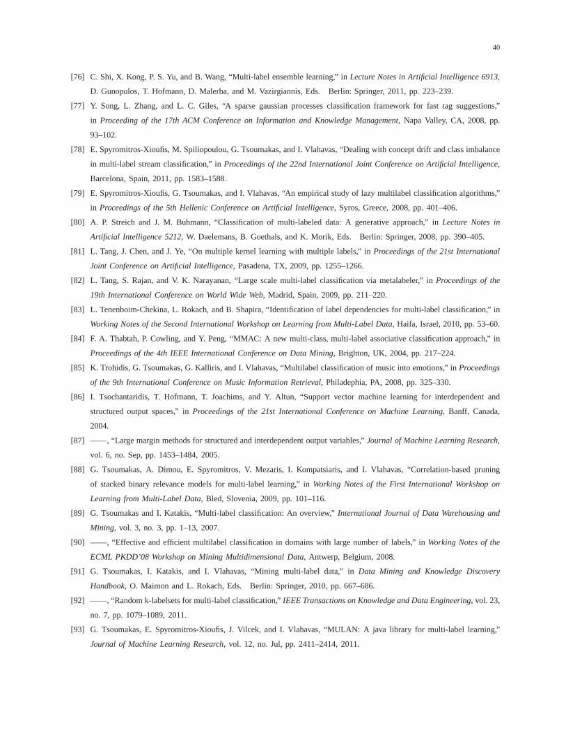
40

[76] C. Shi, X. Kong, P. S. Yu, and B. Wang, “Multi-label ensemble learning,” in Lecture Notes in Artificial Intelligence 6913,

D. Gunopulos, T. Hofmann, D. Malerba, and M. Vazirgiannis, Eds. Berlin: Springer, 2011, pp. 223–239.

[77] Y. Song, L. Zhang, and L. C. Giles, “A sparse gaussian processes classification framework for fast tag suggestions,”

in Proceeding of the 17th ACM Conference on Information and Knowledge Management, Napa Valley, CA, 2008, pp.

93–102.

[78] E. Spyromitros-Xioufis, M. Spiliopoulou, G. Tsoumakas, and I. Vlahavas, “Dealing with concept drift and class imbalance

in multi-label stream classification,” in Proceedings of the 22nd International Joint Conference on Artificial Intelligence,

Barcelona, Spain, 2011, pp. 1583–1588.

[79] E. Spyromitros-Xioufis, G. Tsoumakas, and I. Vlahavas, “An empirical study of lazy multilabel classification algorithms,”

in Proceedings of the 5th Hellenic Conference on Artificial Intelligence, Syros, Greece, 2008, pp. 401–406.

[80] A. P. Streich and J. M. Buhmann, “Classification of multi-labeled data: A generative approach,” in Lecture Notes in

Artificial Intelligence 5212, W. Daelemans, B. Goethals, and K. Morik, Eds. Berlin: Springer, 2008, pp. 390–405.

[81] L. Tang, J. Chen, and J. Ye, “On multiple kernel learning with multiple labels,” in Proceedings of the 21st International

Joint Conference on Artificial Intelligence, Pasadena, TX, 2009, pp. 1255–1266.

[82] L. Tang, S. Rajan, and V. K. Narayanan, “Large scale multi-label classification via metalabeler,” in Proceedings of the

19th International Conference on World Wide Web, Madrid, Spain, 2009, pp. 211–220.

[83] L. Tenenboim-Chekina, L. Rokach, and B. Shapira, “Identification of label dependencies for multi-label classification,” in

Working Notes of the Second International Workshop on Learning from Multi-Label Data, Haifa, Israel, 2010, pp. 53–60.

[84] F. A. Thabtah, P. Cowling, and Y. Peng, “MMAC: A new multi-class, multi-label associative classification approach,” in

Proceedings of the 4th IEEE International Conference on Data Mining, Brighton, UK, 2004, pp. 217–224.

[85] K. Trohidis, G. Tsoumakas, G. Kalliris, and I. Vlahavas, “Multilabel classification of music into emotions,” in Proceedings

of the 9th International Conference on Music Information Retrieval, Philadephia, PA, 2008, pp. 325–330.

[86] I. Tsochantaridis, T. Hofmann, T. Joachims, and Y. Altun, “Support vector machine learning for interdependent and

structured output spaces,” in Proceedings of the 21st International Conference on Machine Learning, Banff, Canada,

2004.

[87] ——, “Large margin methods for structured and interdependent output variables,” Journal of Machine Learning Research,

vol. 6, no. Sep, pp. 1453–1484, 2005.

[88] G. Tsoumakas, A. Dimou, E. Spyromitros, V. Mezaris, I. Kompatsiaris, and I. Vlahavas, “Correlation-based pruning

of stacked binary relevance models for multi-label learning,” in Working Notes of the First International Workshop on

Learning from Multi-Label Data, Bled, Slovenia, 2009, pp. 101–116.

[89] G. Tsoumakas and I. Katakis, “Multi-label classification: An overview,” International Journal of Data Warehousing and

Mining, vol. 3, no. 3, pp. 1–13, 2007.

[90] ——, “Effective and efficient multilabel classification in domains with large number of labels,” in Working Notes of the

ECML PKDD’08 Workshop on Mining Multidimensional Data, Antwerp, Belgium, 2008.

[91] G. Tsoumakas, I. Katakis, and I. Vlahavas, “Mining multi-label data,” in Data Mining and Knowledge Discovery

Handbook, O. Maimon and L. Rokach, Eds. Berlin: Springer, 2010, pp. 667–686.

[92] ——, “Random k-labelsets for multi-label classification,” IEEE Transactions on Knowledge and Data Engineering, vol. 23,

no. 7, pp. 1079–1089, 2011.

[93] G. Tsoumakas, E. Spyromitros-Xioufis, J. Vilcek, and I. Vlahavas, “MULAN: A java library for multi-label learning,”

Journal of Machine Learning Research, vol. 12, no. Jul, pp. 2411–2414, 2011.

41

[94] G. Tsoumakas and I. Vlahavas, “Random k-labelsets: an ensemble method for multilabel classification,” in Lecture Notes

in Artificial Intelligence 4701, J. N. Kok, J. Koronacki, R. L. de Mantaras, S. Matwin, D. Mladenic, and A. Skowron,

Eds. Berlin: Springer, 2007, pp. 406–417.

[95] G. Tsoumakas, M.-L. Zhang, and Z.-H. Zhou, “Tutorial on learning from multi-label data,” in European Conference

on Machine Learning and Principles and Practice of Knowledge Discovery in Databases, Bled, Slovenia, 2009

[http://www.ecml pkdd2009.net/wp-content/uploads/2009/08/learning-from-multi-label-data.pdf].

[96] ——, “Introduction to the special issue on learning from multi-label data,” Machine Learning, vol. 88, no. 1-2, pp. 1–4,

2012.

[97] N. Ueda and K. Saito, “Parametric mixture models for multi-label text,” in Advances in Neural Information Processing

Systems 15, S. Becker, S. Thrun, and K. Obermayer, Eds. Cambridge, MA: MIT Press, 2003, pp. 721–728.

[98] L. C. van der Gaag and P. R. de Waal, “Multi-dimensional Bayesian network classifiers,” in Proceedings of the 3rd

European Workshop in Probabilistic Graphical Models, Prague, Czech Republic, 2006, pp. 107–114.

[99] A. Veloso, W. Meira Jr., M. Goncalves, and M. Zaki, “Multi-label lazy associative classification,” in Lecture Notes in

Artificial Intelligence 4702, J. N. Kok, J. Koronacki, R. L. de Mantaras, S. Matwin, D. Mladenic, and A. Skowron, Eds.

Berlin: Springer, 2007, pp. 605–612.

[100] C. Vens, J. Struyf, L. Schietgat, S. Dzeroski, and H. Blockeel, “Decision trees for hierarchical multi-label classification,”

Machine Learning, vol. 73, no. 2, pp. 185–214, 2008.

[101] H. Wang, C. Ding, and H. Huang, “Multi-label classification: Inconsistency and class balanced k-nearest neighbor,” in

Proceedings of the 24th AAAI Conference on Artificial Intelligence, Atlanta, GA, 2010, pp. 1264–1266.

[102] M. Wang, X. Zhou, and T.-S. Chua, “Automatic image annotation via local multi-label classification,” in Proceedings of

the 7th ACM International Conference on Image and Video Retrieval, Niagara Falls, Canada, 2008, pp. 17–26.

[103] R. Yan, J. Tesic, and J. R. Smith, “Model-shared subspace boosting for multi-label classification,” in Proceedings of the

13th ACM SIGKDD Conference on Knowledge Discovery and Data Mining, San Jose, CA, 2007, pp. 834–843.

[104] Z. Younes, F. Abdallah, T. Denoeux, and H. Snoussi, “A dependent multilabel classification method derived from the

k-nearest neighbor rule,” EURASIP Journal on Advances in Signal Processing, 2011, Article 645964.

[105] J. H. Zaragoza, L. E. Sucar, E. F. Morales, C. Bielza, and P. Larranaga, “Bayesian chain classifiers for multidimensional

classification,” in Proceedings of the 22nd International Joint Conference on Artificial Intelligence, Barcelona, Spain,

2011, pp. 2192–2197.

[106] M.-L. Zhang and K. Zhang, “Multi-label learning by exploiting label dependency,” in Proceedings of the 16th ACM

SIGKDD International Conference on Knowledge Discovery and Data Mining, Washington D. C., 2010, pp. 999–1007.

[107] M.-L. Zhang and Z.-H. Zhou, “Multilabel neural networks with applications to functional genomics and text categoriza-

tion,” IEEE Transactions on Knowledge and Data Engineering, vol. 18, no. 10, pp. 1338–1351, 2006.

[108] ——, “ML-kNN: A lazy learning approach to multi-label learning,” Pattern Recognition, vol. 40, no. 7, pp. 2038–2048,

2007.

[109] ——, “Multi-label learning by instance differentiation,” in Proceedings of the 22nd AAAI Conference on Artificial

Intelligence, Vancouver, Canada, 2007, pp. 669–674.

[110] X. Zhang, Q. Yuan, S. Zhao, W. Fan, W. Zheng, and Z. Wang, “Multi-label classification without the multi-label cost,”

in Proceedings of the 10th SIAM International Conference on Data Mining, Columbus, OH, 2010, pp. 778–789.

[111] Y. Zhang and J. Schneider, “Maximum margin output coding,” in Proceedings of the 29th International Conference on

Machine Learning, Edinburgh, UK, 2012, pp. 1575–1582.

42

[112] Z.-H. Zhou, Ensemble Methods: Foundations and Algorithms. Boca Raton, FL: Chapman & Hall/CRC, 2012.

[113] Z.-H. Zhou, M.-L. Zhang, S.-J. Huang, and Y.-F. Li, “Multi-instance multi-label learning,” Artificial Intelligence, vol.

176, no. 1, pp. 2291–2320, 2012.

[114] S. Zhu, X. Ji, W. Xu, and Y. Gong, “Multi-labelled classification using maximum entropy method,” in Proceedings of

the 28th Annual International ACM SIGIR Conference on Research and Development in Information Retrieval, Salvador,

Brazil, 2005, pp. 274–281.

Multilabel Things

Documents

Transcript of Multilabel Things