
Multihoming: Scheduling, Modelling, and Congestion …ljilja/cnl/guests/Shami-SFU-July-9.pdf ·...
47
-
Upload
duongquynh -
Category
Documents
-
view
215 -
download
0
Transcript of Multihoming: Scheduling, Modelling, and Congestion …ljilja/cnl/guests/Shami-SFU-July-9.pdf ·...


Multihoming: Scheduling, Modelling, and Congestion Window Management
Abdallah Shami T. Daniel Wallace
Simon Fraser University July 2013
Department of Electrical and Computer Engineering

Talk Outline • Motivation/Introduction
• A Review of Multihoming Issues using SCTP*
• CMT: Scheduling
• CMT: Modelling
• CMT: Congestion Window Management
• Conclusion
CMT: Scheduling, Modelling, and CWND Management
*T. D. Wallace, and A. Shami, “A review of multihoming issues using the stream control transmission protocol,” IEEE Communications Surveys & Tutorials, vol. 14, issue 2, pp. 565-578, 2012.
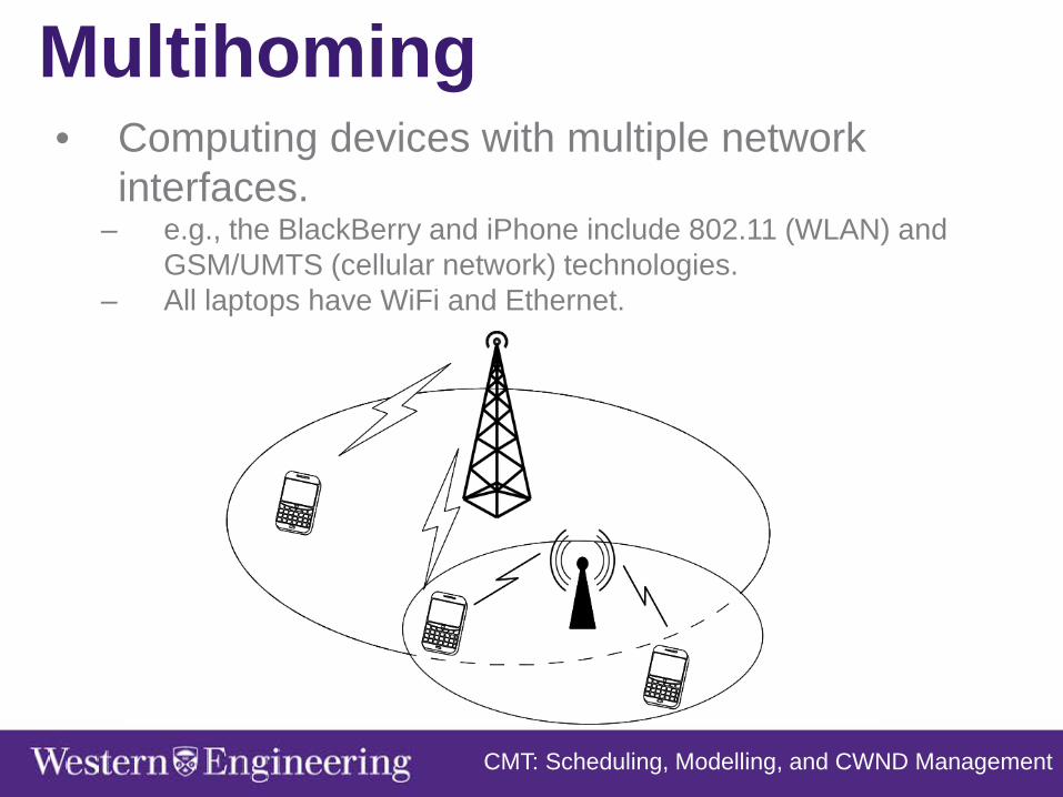
Multihoming • Computing devices with multiple network
interfaces. – e.g., the BlackBerry and iPhone include 802.11 (WLAN) and
GSM/UMTS (cellular network) technologies. – All laptops have WiFi and Ethernet.
CMT: Scheduling, Modelling, and CWND Management

Concurrent Multipath Transfer (CMT) • Goal: Take advantage of multiple network paths, between
end-points, to increase application throughput.
• Architecturally: works from the transport layer in the OSI model.
• Congestion control is managed on a per destination basis, but flow control is handled at the session layer (i.e., only one receive buffer).
CMT: Scheduling, Modelling, and CWND Management

Stream Control Transmission Protocol • An Internet Engineering Task Force (IETF) project
since 2000 (RFC 4960). • Implemented in many operating systems (e.g.,
Linux, Mac OS, FreeBSD, Solaris, Windows). • TCP Similarities:
– Reliable transport protocol. – Ordered delivery. – Implements congestion control and flow control.
• Main difference: SCTP supports multihoming. – Allows application data to be transmitted to multiple IP addresses. – Most useful for vertical handoffs and network faults. – Provides the basics to implement CMT.
CMT: Scheduling, Modelling, and CWND Management

System Description
CMT: Scheduling, Modelling, and CWND Management
Transport Layer Architecture
Multihomed Network Topology
General Terms & Concepts • Congestion Window (CWND)
– A variable that controls the amount of data that can be in flight. • Send Buffer (SBUF)
– The amount of memory allocated to accept data from the application layer before it’s send into the network.
• Receive Buffer (RBUF) – The amount of memory allocated to accept data from the network
before passing it to the application layer. • Receive Window (RWND)
– The available space in the RBUF. • Throughput
– The rate that data arrives at the receiver.
CMT: Scheduling, Modelling, and CWND Management

Multihoming: Problems, Issues, and Challenges
• Handover Management – Preemptive Path Selection – Fault Tolerant Path Selection – Post Handover Synchronization
• Concurrent Multipath Transfer
• Cross Layer Activities – Bandwidth estimation – Wireless error notifications – Network intelligence

Talk Outline • Motivation/Introduction
• A Review of Multihoming Issues using SCTP*
• CMT: Scheduling
• CMT: Modelling
• CMT: Congestion Window Management
• Conclusion
CMT: Scheduling, Modelling, and CWND Management

CMT: Scheduling, Modelling, and CWND Management
CMT: Scheduling • Scheduling & Transmission Basics
• Current Scheduling Approaches for CMT
• On-demand Scheduling
• Performance Results
• Summary & Contributions

Scheduling & Transmission Basics • Data arrives from the application, fragmented into
packets, then waits in the SBUF for a transmission opportunity.
• Transmission opportunities occur when: – 1) CWND must be greater than the number of packets it has in
flight. – 2) RWND is greater than zero.
• Cumulative packet is transmitted. – The packet with lowest sequence number in the SBUF that has yet
to be sent.
CMT: Scheduling, Modelling, and CWND Management

Current Scheduling for CMT • Naïve Round Robin Scheduling*
– No intelligence is used during the scheduling process.
– When only one destination has a transmission opportunity, uses the basic scheduling and transmission technique.
– When multiple destinations have transmission opportunities, packets are transmitted to each destination in a round robin fashion.
CMT: Scheduling, Modelling, and CWND Management
*J. Iyengar, P. Amer, and R. Stewart, “Concurrent multipath transfer using sctp multihoming over independent end-to-end paths,” IEEE/ACM Trans. Netw., vol. 14, no. 5, pp. 951–964, 2006

Current Scheduling for CMT • Naïve Round Robin Scheduling
– Assume bandwidth is the same on either path, but the delay on the
red path is twice as long as the blue path.
– Both paths always have transmission opportunities.
CMT: Scheduling, Modelling, and CWND Management
SBUF
Application Layer
Network Layer
RBUF
Application Layer
Network Layer
Sender
Transport Layer Transport Layer
Receiver
5 3 4 2 1 6 5 3
4 2
1
6
1 5 3 1 5 3 1 3 2 4 6
Receive Buffer Blocking
7 8

Current Scheduling for CMT •Bandwidth Aware Scheduler (BAS)*
– Attempts ordered packet delivery using bandwidth estimates. – Scheduling decisions are made before transmission opportunities – When packets arrive at the SBUF, they are assigned to a
destination’s send queue – Assignments are based on a reception index.
CMT: Scheduling, Modelling, and CWND Management
)()()()()(
dBdSdOpLdR ++
=
n destinatiofor estimatebandwidth a returns)(n destinatiofor queue send in the packets ofnumber thereturns )(n destinatio flight toin bytes)(or packets ofnumber thereturns )(
packet of size thereturns )(addressn destinatio a
packet new a
ddBddSddO
ppLdp
≡≡≡≡
≡≡
* M. Fiore, C. Casetti, and G. Galante, “Concurrent multipath communication for real-time traffic,” Comput. Commun., vol. 30, no. 17, pp. 3307–3320, 2007.

Current Scheduling for CMT • Bandwidth Aware Scheduler
– Assume bandwidth on the red path is twice the speed of the blue’s,
but both experience the same propagation delay.
– Initially, CWND on the red path is only 1 packet.
CMT: Scheduling, Modelling, and CWND Management
SBUF
Application Layer
Network Layer
6 5 3 RBUF
Application Layer
Network Layer
Sender
Transport Layer Transport Layer
Receiver
4 2 1 2 1 6 5 1 2 5 4
3 6
3 4
Packet 3 waits! Packet 6 waits!

On-demand Scheduler • Goal: Find the cumulative packet (in SBUF) that
cannot be delivered to any other destination sooner.
– ODS waits for a transmission opportunity before it makes its
scheduling decision.
– Uses bandwidth and propagation delay to manufacture a packet’s estimated time of acknowledgement (ETA).
– Recursively simulates the transmission and acknowledgement of packets in the SBUF.
CMT: Scheduling, Modelling, and CWND Management

CMT: Scheduling, Modelling, and CWND Management
On-demand Scheduler • Search Algorithm
Copy send buffer.
Find outstanding packet with lowest ETA and
simulate ACK.
Calc ETAs for each destination.
Start a new search. Simulate transmission.

Performance Results • Network Topology
• Simulation
– Implemented each scheduling algorithm in ns-2. – Created a variety of network scenarios to evaluate CMT: delay-
based disparity, bandwidth-based disparity, loss-based disparity, different RBUF sizes.
– Simulated a 1 GB file transfer.
CMT: Scheduling, Modelling, and CWND Management

CMT: Scheduling, Modelling, and CWND Management
Performance Results

CMT: Scheduling, Modelling, and CWND Management
Summary • Developed a new scheduling algorithm for CMT
called On-demand Scheduling (ODS).
• Compared each scheduling algorithm. – ODS will often improve performance, especially when the system is
constrained by a limited RBUF. – BAS is only suitable when the RBUF is very large and preferable
when there is a minor disparity in path delays. – Naïve scheduling is best when there is minimal difference in delays.
• Evaluated ODS under different network scenarios: – delay-based disparity (significant improvement)* – bandwidth-based disparity (some improvement) – loss-based disparity (still an open problem)
*will revisit later

CMT: Scheduling, Modelling, and CWND Management
CMT: Modelling • Modelling Framework
• Markov Model
• Renewal Model
• Performance Results
• Summary & Contributions

CMT: Scheduling, Modelling, and CWND Management
Modelling Framework • Goal:
– Given a multihomed system, approximate the throughput of a long-term session employing CMT.
• Parameters: – bandwidth (per path) – delay (per path) – probability of packet loss (per path) – RBUF size
• Approach: – Model independent SCTP sessions using techniques from TCP
literature, then aggregate throughput predictions. • Assumptions:
– Perfect scheduling. – The CWND must be less than or equal to the RBUF.

CMT: Scheduling, Modelling, and CWND Management
Markov Model •Discrete-time Markov Chain (DTMC)
– SCTP is represented as a set of discrete transmission rounds. – Each round is a state in the Markov chain. – During each round some number of packets are transmitted, where
some or all of those packets might be lost. •States:
– (ω,ξ,τ) – ω = size of the CWND during a round – ξ = number of packets transmitted during a round – τ = slow-start threshold during a round
•Operating Modes: – Congestion Avoidance (CA) – Exponential Backoff (EB) – Slow-start (SS)

CMT: Scheduling, Modelling, and CWND Management
Markov Model • States
• Steady-state probability • Throughput
Q⋅= ππ
( )
{[ ] ( ) ( , ( )) ( ) (1,1)
i
i j iE i jP j j i P
ξ
γ π ξ π∈ ∈
= +∑ ∑ ∑C,S} E
{ , }[ ] ( ) ( ) ( )
i iE i i iξ π ξ π
∈ ∈
= +∑ ∑C S E
[ ] [ ][ ]
E EEξ γη
δ−
=
{ {[ ] ( ) ( , )
i iE i D i iδ π
′∈ ∈
′= ⋅∑ ∑C,S,E} C,S,E}
{ }max( , , ) : 2 ,1 , ,ω ξ τ ω ω ξ ω ω ξ= ≤ ≤ ≤ ≤ ∈ ∈C Z Z
{ }2( , , ) : 2 ,1 log ( ), , 1,i i iω ξ τ ω ξ τ τ τ= = = ≤ ≤ ∈ > ∈S T Z
{ }(0, , ) : 2 , 1) ( 1, )Mξ τ ξ τ ξ τ= ≤ ≤ = ∪ = ∈E T

CMT: Scheduling, Modelling, and CWND Management
Renewal Model • Renewal Theory
– A stochastic process continually restarts at regular intervals. – Formulate a closed-form expression to represent an SCTP session.
• Throughput is approximated by an average interval.
– t = length of time of the average interval – St = number of packets transmitted during the average interval – Lt= number of packets lost during the average interval
• Operating Modes:
– Congestion Avoidance (CA) – Exponential Backoff (EB) – Slow-start (SS)

CMT: Scheduling, Modelling, and CWND Management
Renewal Model • Congestion Avoidance (infinite RBUF, no timeouts)
8(1 ) 1 1[ ]3 9 3
pE Wp−
= + −
2(1 ) 1 5[ ]3 36 6
pE Xp−
= + +
[ ] ( [ ] 1) RTTE T E X= + ⋅
2(1 ) [ ]2 ( [ ] 1) RTT
p E W pp E X
η − + ⋅=
⋅ + ⋅
1[ ] [ ]pE S E Wp−
= +
[ ][ ]2
E WE L =[ ] [ ][ ]
E S E LE T
η −=

CMT: Scheduling, Modelling, and CWND Management
Renewal Model • Exponential Backoff
CA CA TO
CA TO EB
[ ] [ ][ ] [ ]
E S E L PE T P E T
η − +=
+ ⋅
8 4TO 1 (1 ) (1 (1 ) )(1 )
1 (1 )
W
Wp p pP
p− − − − − −
=− −
EBmax
(1 )(1 2 )[ ] RTO RTO1 2 1
M M Mp p pE Tp p
− −= +
− −

CMT: Scheduling, Modelling, and CWND Management
Renewal Model • Slow-start
CA CA TO SS
CA TO EB SS
[ ] [ ] [ ][ ] ( [ ] [ ])
E S E L P E SE T P E T E T
η − + ⋅=
+ +
SS[ ] [ ] 1E S E W= −
SS2[ ] max(1, log [ ]) RTTE T E W= ⋅

CMT: Scheduling, Modelling, and CWND Management
Performance Results

CMT: Scheduling, Modelling, and CWND Management
Summary • Created a tractable framework to model the
throughput of CMT. • Developed two different models based on well-
known techniques: – Discrete-time Markov Chain & Renewal Theory
• Compared the performance of both models with simulated results.
– Markov model is more accurate but suffers from issues of scalability.
– Markov model uses Gaussian Elimination to solve an unbounded matrix.
– Renewal theory is more cost effective, but approximations are not always accurate.
– Renewal theory approximates throughput using a closed-form expression.

CMT: Scheduling, Modelling, and CWND Management
CMT: Congestion Window Management • CWND Update Policy
• CWND Optimization
• Performance Results
• Summary & Contributions

CWND Update Policy • policy1 :SCTP’s current CWND update policy
– SCTP grows its CWND by 1 every RTT. – CWND is unbounded. Even when flow control stops packets from
being transmitted, the CWND continues to grow.
• What impact will policy1 have on CMT? – Lowers utilization and throughput potential. – One destination address can monopolize the RWND.
• Solution – Limit the sum of all CWNDs to the size of the RBUF. – Limit the size of a path’s CWND to its corresponding bandwidth
delay product (BDP). – Apply local or “greedy” optimization.
o Rank destination addresses according to bandwidth potential. o Sets precedence to grow CWND’s of higher ranked destinations first.
CMT: Scheduling, Modelling, and CWND Management

CWND Update Policy • Algorithm name: policy2.
CMT: Scheduling, Modelling, and CWND Management
Limit a destination’s CWND to its BDP.
Sum of CWNDS is less than the RBUF.
Decrease CWND of lower ranked dest when CWND of higher ranked dest Is blocked.

CWND Optimization • Optimal performance (i.e. maximum throughput)
can be linked to the size of each destination’s CWND.
• Two optimization methods: – Dynamic Congestion Window Management (i.e., policy2) – Static Congestion Window Management (ILP and heuristic)
CMT: Scheduling, Modelling, and CWND Management

CWND Optimization • Static Congestion Window Management
– Generate a set of CWND limits to maximize throughput during CMT. – Uses CMT performance model (i.e., Markov or renewal model).
• Integer Linear Program
CMT: Scheduling, Modelling, and CWND Management
),,,,(max maxmaxiiiii
n
itcpdb∑η
∑ ≤n
ii rc ,max
,11 max +⋅≤≤ iii dbcmax ,ic ∈Z
.Ni∈∀ (packets)buffer receive theof size (seconds) path on timeout maximum
(packets) path on limit CWND
(seconds) path on delay second)per (packets path of bandwidth
paths ofnumber
max
max
≡≡
≡
≡≡≡
rit
icid
ibn
i
i
i
i
s.t.

CWND Optimization • Heuristic
– ILP can take a long time to converge. – Heuristic reduces the number of searches needed to find a solution. – Uses a subset of values when searching for the best set of CWND
limits.
CMT: Scheduling, Modelling, and CWND Management
( )
≤+⋅=
≤≤ akdbrakaxkx ii ,1,min,1:
total number of different CWND limits decreases the search space bandwidth on path delay on path
size of the receive buffer
i
i
akb id ir
≡≡≡≡≡

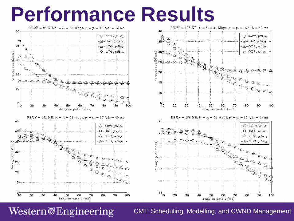
Performance Results • CWND Update Policy
– Revisit delay-based disparity and compare policy1 vs. policy2 • CWND Optimization
– Dynamic vs. Static CWND Management – Heuristic
CMT: Scheduling, Modelling, and CWND Management
CMT: Scheduling, Modelling, and CWND Management
Performance Results

CMT: Scheduling, Modelling, and CWND Management
Performance Results

CMT: Scheduling, Modelling, and CWND Management
Performance Results • Heuristic
– Parameters: r = 128 KB, p1 = p2 = 10-4 ,d1 = d2 = 40 ms, b2 = 10 Mbps, k (variable), b1 (variable).
Higher values of k yield higher throughput.
Lower values of k take less time to find a solution.

CMT: Scheduling, Modelling, and CWND Management
Summary • Developed a new CWND update policy for CMT.
– Compared policy1 to policy2 under delay-based disparity. • Created an ILP to solve the static CWND
management optimization problem. – Compared dynamic and static CWND management under different
network scenarios. – Static CWND management yields better results but requires system
knowledge (e.g, loss rate) and increases computational complexity. • Reduced computational complexity by developing
a simple heuristic. – Evaluated our heuristic using various subsets of CWND limits. – Using larger values of k lowers performance capabilities but also
reduces computational requirements.

CMT: Scheduling, Modelling, and CWND Management
Open Challenges

CMT: Scheduling, Modelling, and CWND Management
Challenges • CMT: Scheduling
– Problem: ODS is a search algorithm that has some computational
requirements.
– Develop a closed-form expression that imitates ODS.
– Implement ODS in the Linux kernel.

CMT: Scheduling, Modelling, and CWND Management
Open Challenges • CMT: Modelling
– Problem: perfect scheduling was assumed to avoid receive buffer
blocking due to loss-based disparity.
– Incorporate the effects of loss-based disparity into the model.

CMT: Scheduling, Modelling, and CWND Management
Open Challenges • CMT: CWND Management
– Problem: short term gains are not considered during the static
optimization process.
– Include the short term gains into the CMT model for static CWND management.
– Develop a solution method using a metaheurstic (e.g., simulated
annealing, tabu search, genetic algorithms).
– Formulate an optimal decision policy using a Markov Decision Process (MDP).