Multidisciplinary Design Analysis and Optimisation of … Governing Equations of Solid Structure ......

Multidisciplinary Design Analysis and Optimisationof Rear Wings for Sports Cars

Miguel da Silva Ferreira

Thesis to obtain the Master of Science Degree in

Aerospace Engineering

Supervisor: Prof. André Calado Marta

Examination Committee

Chairperson: Prof. Filipe Szolnoky Ramos Pinto Cunha

Supervisor: Prof. André Calado Marta

Member of the Committee: Prof. Miguel António Lopes de Matos Neves

June 2016

Acknowledgments

I would like to thank Prof. Andre Marta for his knowledge and guidance throughout the elaboration of

this dissertation.

I would also like to thank Prof. Miguel Matos Neves, for his support and in introducing me to the

CAD/FEM team of the Instituto de Plasmas e Fusao Nuclear (IPFN). A special thank you to the IPFN,

in allowing me to use an ANSYS R© License to achieve the proposed objectives of this dissertation. In

particular, to Prof. Hugo Policarpo for special motivation, guidance, and provide all the means at its

disposal to help me with the varied ANSYS R© related obstacles faced. Also to Paulo Quental, IPFN

researcher, for his disposal in always helping me with the several challenges faced.

This project was a culmination of the last six years of completing my degree which would not be

possible without my friends, and the friends made in this time. A very special thank you to Iuri Figueiredo,

for the companion and support in the last months of the course of this dissertation.

To Maria Pissarra, for all the affection and support in the hardest times.

To my family, I am deeply grateful for the continued knowledge and support in all my endeavors.

Finally, I would like the express my deep love to my Godfather, Anibal da Silva, one of the most

incredible and wonderful persons I have ever met. This dissertation is dedicated to him.

iii

Resumo

A presente dissertacao apresenta uma optimizacao aero-structural de designs de asas traseiras in-

vertidas para minimizar a resistencia aerodinamica e a massa estrutural. Dado que estes dispositivos

tem uma elevada influencia na performance de veıculos, de modo a obter designs optimos eficazes e

seguros, a multifısica envolvida foi assegurada atraves da interaccao fluido-estrutura.

O principal objectivo foi desenvolver a implementacao de uma metodologia para o design de dispos-

itivos aerodinamicos automoveis optimos. Para resolver o problema de optimizacao aero-estrutural, foi

aplicada uma plataforma de projecto, analise e optimizacao multidisciplinar. Dois casos de estudo foram

considerados: uma estrategia de design convencional utilizada em aplicacoes automoveis gerais e de-

sportivas; e um design proposto, onde a superfıcie de conexao entre as placas laterais e os suportes

verticais e utilizada para gerar sustentacao negativa adicional.

Para assegurar a sinergia multidisciplinar e obter solucoes fidedignas, um software de engenharia

assistida por computador foi utilizado (ANSYS R© Workbench 14.5).

O projecto foi dividido em tres partes: as configuracoes dos diferentes modelos numericos, os es-

tudos parametricos aerodinamicos e estruturais (focados nos efeitos das variaveis de projecto) e as

optimizacoes aerodinamicas e estruturais (focadas nas variaveis de maior impacto) para obter designs

optimos.

A partir dos estudos realizados nesta dissertacao, uma plataforma de design analise e optimizacao

multidisciplinar foi desenvolvida para o design preliminar de asas traseiras invertidas, o qual pode ser

tambem aplicado a quaisquer outros dispositivos aerodinamicos automoveis. Geracao da malha e

a modelacao da turbulencia sao aspectos importantes no que respeita a qualidade e precisao das

solucoes numericas e para problemas com deformacoes pequenas, usando uma estrategia one-way

de interaccao fluido-estrutura tem vantages computacionais significativas.

Palavras-chave: Problema aero-estrutural, Interaccao fluido-estrutura, Engenharia assistida

por computador, Dispositivos aerodinamicos, Materiais compositos.

v

Abstract

This thesis covers aero-structural optimisation of rear wing designs to minimise aerodynamic drag and

structural mass. These structures highly influence the performance of vehicles, and in order to achieve

effective and safe optimal designs, the multiphysics involved was considered by means of fluid-structure

interaction (FSI).

The objective was to fold the implementation of a process for optimal automotive aerodynamic de-

vices design. To solve the aero-structural optimisation problem, a multidisciplinary design analysis and

optimisation (MDAO) framework was applied. Two study cases were considered: a traditional rear wing

design strategy used in automotive and motorsport applications; and a proposed design, where the

surface connection between the endplates and vertical supports is used to create additional downforce.

Concerning the multidisciplinary synergy to obtain feasible solutions, a Computer Aided Engineering

(CAE) software was used (ANSYS R© Workbench 14.5).

The project was divided into three parts: the numerical models settings, the aerodynamic and struc-

tural parametric studies (focused on the effects of the design variables), and aerodynamic and structural

optimisation problems (focused on the most impacting variables) to obtain optimal designs.

From the studies performed in this thesis, a MDAO process for optimal preliminary design was de-

veloped for rear wings, but it can also be applied to any other automotive aerodynamic devices. Mesh

and turbulence modelling strategy proved to be very important regarding the accuracy of the numerical

solutions and for problems with small deformations, a one-way FSI coupling technique has significant

computational advantages.

Keywords: Aero-structural problem, Fluid-structure interaction, Computer-aided engineering,

Aerodynamic devices, Composite materials.

vii

Contents

Acknowledgments . . . . . . . . . . . . . . . . . . . . . . . . . . . . . . . . . . . . . . . . . . . iii

Resumo . . . . . . . . . . . . . . . . . . . . . . . . . . . . . . . . . . . . . . . . . . . . . . . . . v

Abstract . . . . . . . . . . . . . . . . . . . . . . . . . . . . . . . . . . . . . . . . . . . . . . . . . vii

Contents . . . . . . . . . . . . . . . . . . . . . . . . . . . . . . . . . . . . . . . . . . . . . . . . xi

List of Tables . . . . . . . . . . . . . . . . . . . . . . . . . . . . . . . . . . . . . . . . . . . . . . xiii

List of Figures . . . . . . . . . . . . . . . . . . . . . . . . . . . . . . . . . . . . . . . . . . . . . xv

Nomenclature . . . . . . . . . . . . . . . . . . . . . . . . . . . . . . . . . . . . . . . . . . . . . . xix

Glossary . . . . . . . . . . . . . . . . . . . . . . . . . . . . . . . . . . . . . . . . . . . . . . . . xxiii

1 Introduction 1

1.1 Motivation . . . . . . . . . . . . . . . . . . . . . . . . . . . . . . . . . . . . . . . . . . . . . 1

1.2 Rear Wing Optimal Design . . . . . . . . . . . . . . . . . . . . . . . . . . . . . . . . . . . 2

1.2.1 Design Considerations . . . . . . . . . . . . . . . . . . . . . . . . . . . . . . . . . . 2

1.2.2 Multidisciplinary Design Analysis and Optimisation Framework . . . . . . . . . . . 4

1.3 Thesis Objectives . . . . . . . . . . . . . . . . . . . . . . . . . . . . . . . . . . . . . . . . . 5

1.4 Dissertation Structure . . . . . . . . . . . . . . . . . . . . . . . . . . . . . . . . . . . . . . 6

2 Automotive Aerodynamics 7

2.1 History of Aerodynamics in Performance Cars Design . . . . . . . . . . . . . . . . . . . . 7

2.1.1 The Impact of Motorsport Aerodynamics on Production Cars . . . . . . . . . . . . 9

2.2 Performance Cars Aerodynamic Devices . . . . . . . . . . . . . . . . . . . . . . . . . . . . 9

2.2.1 Vehicle’s Front-End . . . . . . . . . . . . . . . . . . . . . . . . . . . . . . . . . . . . 9

2.2.2 Vehicle’s Under-body . . . . . . . . . . . . . . . . . . . . . . . . . . . . . . . . . . 11

2.2.3 Vehicle’s Back-End . . . . . . . . . . . . . . . . . . . . . . . . . . . . . . . . . . . . 12

2.3 Methods used for Evaluating Automotive Performance . . . . . . . . . . . . . . . . . . . . 13

2.3.1 Numerical Simulations . . . . . . . . . . . . . . . . . . . . . . . . . . . . . . . . . . 14

2.3.2 Wind Tunnel Testing . . . . . . . . . . . . . . . . . . . . . . . . . . . . . . . . . . . 14

2.3.3 Road and Track Testing . . . . . . . . . . . . . . . . . . . . . . . . . . . . . . . . . 15

3 Theoretical Background 17

3.1 Aerodynamic Theory . . . . . . . . . . . . . . . . . . . . . . . . . . . . . . . . . . . . . . . 17

3.1.1 Governing Equations of Fluid Flow . . . . . . . . . . . . . . . . . . . . . . . . . . . 17

ix

3.1.2 Turbulent Flows and Turbulence Modelling . . . . . . . . . . . . . . . . . . . . . . . 18

3.2 Structures Theory . . . . . . . . . . . . . . . . . . . . . . . . . . . . . . . . . . . . . . . . 21

3.2.1 Governing Equations of Solid Structure . . . . . . . . . . . . . . . . . . . . . . . . 21

3.2.2 First-Order Deformation Theory . . . . . . . . . . . . . . . . . . . . . . . . . . . . . 22

3.3 Fluid-Structure Interaction (FSI) . . . . . . . . . . . . . . . . . . . . . . . . . . . . . . . . . 23

3.3.1 Monolithic and Partitioned Methods . . . . . . . . . . . . . . . . . . . . . . . . . . 24

3.4 Multidisciplinary Design Analysis and Optimisation (MDAO) . . . . . . . . . . . . . . . . . 26

3.4.1 MDAO Architectures . . . . . . . . . . . . . . . . . . . . . . . . . . . . . . . . . . . 26

3.4.2 Numerical Optimisation Techniques . . . . . . . . . . . . . . . . . . . . . . . . . . 26

4 Methodology and Numerical Models 29

4.1 MDAO in ANSYS R© Workbench 14.5 . . . . . . . . . . . . . . . . . . . . . . . . . . . . . . 29

4.2 CAD Model: ANSYS R© DesignModeler . . . . . . . . . . . . . . . . . . . . . . . . . . . . . 30

4.3 CFD Model: ANSYS R© Fluent . . . . . . . . . . . . . . . . . . . . . . . . . . . . . . . . . . 30

4.3.1 Model Validation with NACA 4415 Airfoil Two-Dimensional Analyses . . . . . . . . 31

4.3.2 Benzing BE 122-125 Airfoil Three-Dimensional Analyses . . . . . . . . . . . . . . 36

4.4 CSM Model: ANSYS R© Composite PrepPost and Mechanical . . . . . . . . . . . . . . . . 39

4.4.1 Finite Element Analysis Setup . . . . . . . . . . . . . . . . . . . . . . . . . . . . . 39

4.5 FSI Model: ANSYS R© System Coupling . . . . . . . . . . . . . . . . . . . . . . . . . . . . 43

4.5.1 One-Way versus Two-Way Coupling . . . . . . . . . . . . . . . . . . . . . . . . . . 44

4.6 Optimisation Model: ANSYS R© Direct Optimisation . . . . . . . . . . . . . . . . . . . . . . 46

5 Results 51

5.1 MDAO Design Variables and Functions of Interest . . . . . . . . . . . . . . . . . . . . . . 51

5.2 CAD Parametric Design . . . . . . . . . . . . . . . . . . . . . . . . . . . . . . . . . . . . . 53

5.2.1 Airfoil Selection . . . . . . . . . . . . . . . . . . . . . . . . . . . . . . . . . . . . . . 53

5.2.2 Endplate Design . . . . . . . . . . . . . . . . . . . . . . . . . . . . . . . . . . . . . 54

5.2.3 Vertical Wing Support Design . . . . . . . . . . . . . . . . . . . . . . . . . . . . . . 55

5.2.4 Flow Design . . . . . . . . . . . . . . . . . . . . . . . . . . . . . . . . . . . . . . . 56

5.2.5 Parameters . . . . . . . . . . . . . . . . . . . . . . . . . . . . . . . . . . . . . . . . 56

5.3 Aerodynamic Parametric Studies . . . . . . . . . . . . . . . . . . . . . . . . . . . . . . . . 57

5.3.1 Effect of Horizontal and Vertical Positioning of Lower Wings . . . . . . . . . . . . . 58

5.3.2 Effect of Chord, Wingspan and Angle of Attack . . . . . . . . . . . . . . . . . . . . 60

5.3.3 Effect of Endplates Dimensions . . . . . . . . . . . . . . . . . . . . . . . . . . . . . 64

5.3.4 Vertical Supports Positioning . . . . . . . . . . . . . . . . . . . . . . . . . . . . . . 65

5.4 Aerodynamic Optimisation . . . . . . . . . . . . . . . . . . . . . . . . . . . . . . . . . . . . 66

5.5 One-Way FSI Structural Parametric Studies . . . . . . . . . . . . . . . . . . . . . . . . . . 69

5.5.1 Effect of Material Type . . . . . . . . . . . . . . . . . . . . . . . . . . . . . . . . . . 69

5.5.2 Effect of Number and Orientation of Composite Plies . . . . . . . . . . . . . . . . . 70

5.6 One-Way FSI Structural Optimisation . . . . . . . . . . . . . . . . . . . . . . . . . . . . . . 73

x

5.7 Reduced/Finer Mesh Models and Final Results . . . . . . . . . . . . . . . . . . . . . . . . 75

6 Conclusions 81

6.1 Analyses Conclusions and Recommendations . . . . . . . . . . . . . . . . . . . . . . . . 81

6.2 Future Work . . . . . . . . . . . . . . . . . . . . . . . . . . . . . . . . . . . . . . . . . . . . 82

Bibliography 83

A Chapter 5 Data 89

A.1 Additional Aerodynamic Parametric Studies . . . . . . . . . . . . . . . . . . . . . . . . . . 89

A.1.1 Effect of Wingspan Variation . . . . . . . . . . . . . . . . . . . . . . . . . . . . . . 89

A.1.2 Effect of Angle of Attack Variation . . . . . . . . . . . . . . . . . . . . . . . . . . . 90

A.1.3 Effect of Endplates Dimensions Variation . . . . . . . . . . . . . . . . . . . . . . . 92

A.1.4 Effect of Vertical Supports Positioning . . . . . . . . . . . . . . . . . . . . . . . . . 94

A.2 One-Way FSI Structural Optimisation . . . . . . . . . . . . . . . . . . . . . . . . . . . . . . 95

A.3 Final Results and Designs Comparison . . . . . . . . . . . . . . . . . . . . . . . . . . . . 97

B Material Properties Data Sheets 99

xi

List of Tables

4.1 Fluid flow reference values and target experimental data. . . . . . . . . . . . . . . . . . . 31

4.2 Spatial discretisation schemes selected for the numerical analyses using ANSYS R© Fluent. 32

4.3 Boundary conditions settings for the numerical analyses using ANSYS R© Fluent. . . . . . 32

4.4 NACA 4415 mesh dependency investigations for airfoil number of divisions, using γ-Reθt

transition model, compared to experimental data from [61]. . . . . . . . . . . . . . . . . . 35

4.5 NACA 4415 mesh dependency investigations for inflation options, using γ-Reθt transition

model, compared to experimental data from [61]. . . . . . . . . . . . . . . . . . . . . . . . 35

4.6 Comparison of turbulence modelling influence for test case ’XXIV’ against experimental

data. . . . . . . . . . . . . . . . . . . . . . . . . . . . . . . . . . . . . . . . . . . . . . . . . 36

4.7 Three-dimensional fluid flow reference values for ANSYS R© Fluent and wing dimensions,

using Benzing BE 122-125 airfoil. . . . . . . . . . . . . . . . . . . . . . . . . . . . . . . . . 37

4.8 Three-dimensional fluid flow studies with Fluent for different turbulence modelling and

meshing strategies. . . . . . . . . . . . . . . . . . . . . . . . . . . . . . . . . . . . . . . . . 39

4.9 Three-dimensional wing mesh dependency investigations with ACP and Mechanical for

SHELL181 and SHELL281 elements with one-way FSI coupling technique. . . . . . . . . 42

4.10 Approximate values of the computational time when performing FSI analyses using differ-

ent available coupling techniques in ANSYS R© Workbench for the plate exposed to wind

flow test case. . . . . . . . . . . . . . . . . . . . . . . . . . . . . . . . . . . . . . . . . . . . 46

5.1 Variables and functions of interest for the MDAO process . . . . . . . . . . . . . . . . . . 52

5.2 Baseline design variables (parameters) values assigned for the rear wings. . . . . . . . . 53

5.3 Endplates effect in wing downforce, drag and efficiency. . . . . . . . . . . . . . . . . . . . 55

5.4 Baseline aerodynamic performance values of the traditional and proposed rear wings. . . 57

5.5 Proposed rear wing lower wings horizontal position effect. . . . . . . . . . . . . . . . . . . 58

5.6 Proposed rear wing lower wings vertical position effect. . . . . . . . . . . . . . . . . . . . 60

5.7 Traditional rear wing profile chord effect. . . . . . . . . . . . . . . . . . . . . . . . . . . . . 61

5.8 Proposed rear wing main wing profile chord effect. . . . . . . . . . . . . . . . . . . . . . . 61

5.9 Proposed rear wing lower wings profile chord effect. . . . . . . . . . . . . . . . . . . . . . 61

5.10 Traditional rear wing angle of attack effect. . . . . . . . . . . . . . . . . . . . . . . . . . . . 62

5.11 Proposed rear wing main wing angle of attack effect. . . . . . . . . . . . . . . . . . . . . . 62

5.12 Proposed rear wing lower wings angle of attack effect. . . . . . . . . . . . . . . . . . . . . 62

xiii

5.13 Traditional rear wing vertical supports position effect. . . . . . . . . . . . . . . . . . . . . . 65

5.14 Proposed rear wing vertical supports position effect. . . . . . . . . . . . . . . . . . . . . . 65

5.15 Initial design variables values (1st. design point). . . . . . . . . . . . . . . . . . . . . . . . 66

5.16 Objective and constraint functions and design variables definition for the rear wings aero-

dynamic optimisation using the NLPQL algorithm. . . . . . . . . . . . . . . . . . . . . . . 67

5.17 Traditional rear wing aerodynamic optimisation results. (Note the highlighted best candi-

date design). . . . . . . . . . . . . . . . . . . . . . . . . . . . . . . . . . . . . . . . . . . . 67

5.18 Proposed rear wing aerodynamic optimisation results. (Note the highlighted best candi-

date design). . . . . . . . . . . . . . . . . . . . . . . . . . . . . . . . . . . . . . . . . . . . 68

5.19 Rear wings candidate point 1 aerodynamic performance values for 90 m/s. . . . . . . . . 69

5.20 Effect of the type of material for the traditional rear wing design. . . . . . . . . . . . . . . . 69

5.21 Effect of the number of plies for the traditional rear wing using the RC200T woven prepreg. 70

5.22 Effect of the number of plies for the proposed rear wing using the RC200T woven prepreg. 71

5.23 Effect of the plies orientation for the traditional rear wing using the RC200T woven prepreg. 71

5.24 Effect of the plies orientation for the proposed rear wing using the RC200T woven prepreg. 71

5.25 Objective function, constraint functions and design variables definition for the rear wings

structural optimisation using the MISQP algorithm. . . . . . . . . . . . . . . . . . . . . . . 73

5.26 Traditional rear wing structural optimisation results for minimisation of mass, using sets of

[(45,90)n]s for the stacking sequence of Wing Skin/Wing Spars/Endplates. . . . . . . . . . 74

5.27 Proposed Rear Wing structural optimisation results for minimisation of mass, using sets of

[(30,90)n]s for the stacking sequence of MW Skin/LW Skin/MW Spars/LW Spars/Endplates. 74

5.28 Proposed Rear Wing 2nd. structural optimisation results for minimisation of maximum

deformation. . . . . . . . . . . . . . . . . . . . . . . . . . . . . . . . . . . . . . . . . . . . 75

5.29 Traditional rear wing design aerodynamic (50 m/s) and structural (90 m/s) performance

results comparison between the coarse/fine mesh strategy. . . . . . . . . . . . . . . . . . 76

5.30 Proposed rear wing design aerodynamic (50 m/s) and structural (90 m/s) performance

results comparison between the coarse/fine mesh strategy. . . . . . . . . . . . . . . . . . 76

5.31 Rear Wing designs performance comparison. . . . . . . . . . . . . . . . . . . . . . . . . . 78

A.1 Traditional rear wing span effect. . . . . . . . . . . . . . . . . . . . . . . . . . . . . . . . . 89

A.2 Proposed Rear Wing main wing span effect. . . . . . . . . . . . . . . . . . . . . . . . . . . 89

A.3 Traditional Rear Wing endplates length effect. . . . . . . . . . . . . . . . . . . . . . . . . . 92

A.4 Proposed Rear Wing endplates length effect. . . . . . . . . . . . . . . . . . . . . . . . . . 92

A.5 Traditional Rear Wing endplates upper distance effect. . . . . . . . . . . . . . . . . . . . . 92

A.6 Proposed Rear Wing endplates upper distance effect. . . . . . . . . . . . . . . . . . . . . 92

A.7 Traditional Rear Wing endplates lower distance effect. . . . . . . . . . . . . . . . . . . . . 93

A.8 Proposed Rear Wing endplates lower distance effect. . . . . . . . . . . . . . . . . . . . . 93

B.1 Properties of the materials used in this dissertation. . . . . . . . . . . . . . . . . . . . . . 100

xiv

List of Figures

1.1 Designed rear wing for Structural Mechanics course assembled in a Porsche Carrera GT. 2

1.2 MDAO framework established for the aero-structural optimisation problem. . . . . . . . . . 5

2.1 Introduction of ground effect by F1 Lotus team in 1977 [11]. . . . . . . . . . . . . . . . . . 8

2.2 Trends showing the increase of the maximum cornering acceleration over the past years

for race cars with and without aerodynamic downforce [1]. . . . . . . . . . . . . . . . . . . 8

2.3 Examples of hypercars with aerodynamic devices influenced by motorsport. . . . . . . . . 9

2.4 Downforce and drag coefficient versus ground clearance for an inverted LS(1)-0413 airfoil

[15]. . . . . . . . . . . . . . . . . . . . . . . . . . . . . . . . . . . . . . . . . . . . . . . . . 10

2.5 Interaction between the rear wing and the car body [21]. . . . . . . . . . . . . . . . . . . . 13

3.1 Subdivisions of the flow near-wall region [31]. . . . . . . . . . . . . . . . . . . . . . . . . . 20

3.2 Solution strategies for FSI problems. . . . . . . . . . . . . . . . . . . . . . . . . . . . . . . 24

3.3 Solution algorithm for weak one-way and two-way coupling systems. . . . . . . . . . . . . 25

3.4 Illustration of Response Surface Optimisation Methodology [51]. . . . . . . . . . . . . . . 28

4.1 Example of a MDAO project schematic in ANSYS R© Workbench. . . . . . . . . . . . . . . 30

4.2 Virtual wind tunnel geometry and an example of the hybrid mesh applied to the fluid flow

geometry in ANSYS R© Fluent. . . . . . . . . . . . . . . . . . . . . . . . . . . . . . . . . . . 33

4.3 Three dimensional virtual wind tunnel geometry and mesh of test case ’I’ (with γ-Reθt

transition model). . . . . . . . . . . . . . . . . . . . . . . . . . . . . . . . . . . . . . . . . . 37

4.4 Closer look at the airfoil mesh for optimisation test cases ’IV Opt.’ using γ-Reθt model

and ’VI Opt.’ using realizable k-ǫ model with non-equilibrium wall functions in ANSYS R©

Meshing. . . . . . . . . . . . . . . . . . . . . . . . . . . . . . . . . . . . . . . . . . . . . . 38

4.5 Benzing BE 122-125 wing profile, double spars and assembled endplates geometry and

mesh for test case ’Mesh I’. . . . . . . . . . . . . . . . . . . . . . . . . . . . . . . . . . . . 41

4.6 Test case geometry used to assess the computational effort for different FSI coupling

techniques and the solution process to solve FSI analyses for thin structures. . . . . . . . 45

4.7 Plate section view of Inflation mesh option for the thin and hollow plate. . . . . . . . . . . 45

5.1 Example of a conventional and ’idealised’ proposed design of rear wings to be studied

and optimised in this dissertation. . . . . . . . . . . . . . . . . . . . . . . . . . . . . . . . . 51

xv

5.2 Baseline parametrised rear wings geometries used for the parametric studies. . . . . . . 53

5.3 Effect of the angle of attack in the airfoil efficiency. . . . . . . . . . . . . . . . . . . . . . . 54

5.4 Endplates effect visualised by surface streamlines (wall shear stress patterns) near the

wing tip region. . . . . . . . . . . . . . . . . . . . . . . . . . . . . . . . . . . . . . . . . . . 55

5.5 Virtual wind tunnel geometry example of the baseline proposed rear wing. . . . . . . . . . 56

5.6 Effect of backward position of lower wings relative to the main wing (+0.20 m) visualised

by surface (wall shear stress patterns) and flow velocity streamlines. . . . . . . . . . . . . 59

5.7 Effect of varying the main wing and lower wings angle of attack by visualisation of the

surface streamlines (wall shear stress patterns), for the realizable k-ǫ turbulence model. . 63

5.8 Convergence plots of the objective and constraint function for the traditional rear wing

optimisation problem, using the NLPQL algorithm. . . . . . . . . . . . . . . . . . . . . . . 67

5.9 Convergence plots of the objective and constraint function for the proposed rear wing

optimisation problem, using the NLPQL algorithm. . . . . . . . . . . . . . . . . . . . . . . 68

5.10 Structural response of the traditional and proposed rear wings for a laminate stacking

sequence of [(90)8] and [(90)16], respectively. . . . . . . . . . . . . . . . . . . . . . . . . . 72

5.11 Structural response of the traditional rear wing Candidate point 1 and 2 (10 : 1 scale). . . . 74

5.12 Traditional rear wing upper and lower sides pressure distribution and surface streamlines

for the coarse and refined mesh model at a flow velocity of 50 m/s. . . . . . . . . . . . . . 77

5.13 Concept high-performance cars with similar rear wing design strategy. . . . . . . . . . . . 79

A.1 Effect of varying the wing angle of attack of the traditional rear wing, by visualisation of

the surface pressure distribution and streamlines (wall shear stress patterns), using the

realizable k-ǫ turbulence model. . . . . . . . . . . . . . . . . . . . . . . . . . . . . . . . . . 90

A.2 Effect of varying the proposed design main wing angle of attack to 5 deg by visualisation

of the surface streamlines (wall shear stress patterns), using the realizable k-ǫ turbulence

model. . . . . . . . . . . . . . . . . . . . . . . . . . . . . . . . . . . . . . . . . . . . . . . . 91

A.3 Effect of varying the main wing and lower wings angle of attack by visualisation of the

surface pressure distribution, using the realizable k-ǫ turbulence model. . . . . . . . . . . 91

A.4 Pressure distribution of the proposed rear wing design for the effect of vertical supports

positioning, using the with realizable k-ǫ turbulence model. . . . . . . . . . . . . . . . . . . 94

A.5 Convergence plots of the objective and constraint function for the traditional rear wing

optimisation problem for the minimisation of mass, using the MISQP algorithm. . . . . . . 95

A.6 Convergence plots of the objective and constraint function for the proposed rear wing

optimisation problem for the minimisation of mass, using the MISQP algorithm. . . . . . . 95

A.7 Convergence plots of the objective and constraint function for the proposed rear wing

optimisation problem for the minimisation of maximum deformation, using the MISQP

algorithm. . . . . . . . . . . . . . . . . . . . . . . . . . . . . . . . . . . . . . . . . . . . . . 96

xvi

A.8 Traditional rear wing Candidate Point 1 residuals statiscs and convergence for the coarse

and refined mesh model (Test Case ’VI Opt.’ and ’II’ with realizable k-ǫ model application,

respectively). . . . . . . . . . . . . . . . . . . . . . . . . . . . . . . . . . . . . . . . . . . . 97

xvii

Nomenclature

Greek symbols

α Angle of attack.

∆ Relative variation.

ǫ Turbulent dissipation.

γ Intermittency.

κ Turbulent kinetic energy.

µ Fluid dynamic viscosity.

ν Fluid kinematic viscosity.

ω Specific dissipation.

ρ Density.

σ Stress.

τ Shear stress.

ε Strain.

Roman symbols

A Aspect ratio.

BF Bias factor.

CD Three-dimensional coefficient of drag.

Cd Two-dimensional coefficient of drag.

CL Three-dimensional coefficient of lift.

Cl Two-dimensional coefficient of lift.

Cm Two-dimensional coefficient of moment.

C Global damping matrix.

xix

D Drag force.

d Displacement.

FC Failure criterion.

g Body accelerations acting on the continuum (per unit mass).

GT Growth rate.

−L Downforce.

−L/D Downforce-to-drag ratio.

LB Lower bound.

LW Lower wings.

M Global mass matrix.

MW Main wing.

NE Number of elements.

NL Number of prismatic layers.

p Pressure.

PC Wing profile chord.

PL Vertical supports position from symmetry plane.

PRW Proposed rear wing.

Q Global stiffness matrix.

Re Reynolds number.

TRW Traditional rear wing.

TT Total thickness.

u Velocity vector.

U Fluid velocity.

u, v, w Velocity Cartesian components.

Umax Maximum Deformation.

UB Upper bound.

VS Vertical supports.

y+ Dimensionless wall distance.

xx

Subscripts

1 Longitudinal fibre direction.

2 Transverse fibre direction.

w Wall.

x, y, z Cartesian components.

Superscripts

◦ Middle plane.

f Fluid interface.

s Solid interface.

xxi

Glossary

CAD Computer-Aided Design is the use of computer

systems to aid in the creation, modification,

analysis, or optimization of a design.

CAE Computer-Aided Engineering is the broad us-

age of computer software to aid in engineering

analysis tasks, including CSM, CFD, multibody

dynamics and optimisation.

CFD Computational Fluid Dynamics is a branch of

fluid mechanics that uses numerical methods

and algorithms to solve problems that involve

fluid flows.

CFRTP Carbon-Fiber-Reinforced Thermoplastic is a

strong and light fiber-reinforced plastic which

contains carbon fibres.

CSM Computational Structural Mechanics is a

branch of structure mechanics that uses nu-

merical methods and algorithms to perform the

analysis of structures and its components.

FEM Finite Element Method is a numerical technique

for finding approximate solutions to boundary

value problems for partial differential equations,

usually used by CSM software. It is also re-

ferred to as finite element analysis (FEA).

FSDT First-Order Shear Deformation Theory is usu-

ally applied for modelling composite shells or

sandwich construction of layered applications.

FSI Fluid-Structure Interaction is the interaction of

some movable or deformable structure with an

internal or surrounding fluid flow.

xxiii

MDAO Multidisciplinary Design Analysis and Optimi-

sation is an engineering technique that uses

optimisation methods to solve design problems

incorporating two or more disciplines.

MISQP Mixed-Integer Sequential Quadratic Program-

ming is an optimisation solver that handles

dense mixed-integer non-linear programming

problems by a modified sequential quadratic

programming method.

NLPQL Non-Linear Programming by Quadratic La-

grangian is an optimisation gradient based sin-

gle objective optimiser which solves smooth

non-linear programming problems by a sequen-

tial quadratic programming method.

SQP Sequential Quadratic Programming is an itera-

tive method for non-linear optimisations, which

solve a sequence of optimization subproblems,

each of which optimises a quadratic model of

the objective subject to a linearisation of the

constraints.

xxiv

Chapter 1

Introduction

1.1 Motivation

With the desire to go faster than ever before, the automotive industry consistently benefits of engineering

and technology progress. In engineering, depending on its application, usually the end goal of any work

is optimisation. Whether it be increasing the efficiency of a rear wing, or proper placement of material to

reduce weight, such optimisation process is as much of an art as it is a science.

Aerodynamic and structural effectiveness are two of the most important subjects that affect the per-

formance of vehicles. In the late 1960s, several teams started to use wings in their race cars and it was

at this point that aerodynamics began to play a key role in race car design. Nowadays, aerodynamic

upgrades come in many different forms and devices, yet, in motorsport and sports car technology, wings

have an essential function in the exploitation of downforce. Essentially, aerodynamicists have two pri-

mary concerns [1, 2]: at first the creation of downforce, a virtual weight that helps pushing the car tires

onto the track improving stability and cornering forces, and second, the minimisation of drag, a product

of air resistance which acts to slow the car down.

Fibre-reinforced composites are often more profitable and efficient than conventional materials due

to their high strength-to-weight ratio and the possibility of adapting their stiffness by selecting fibre ori-

entations [3]. Because of this, their use in mechanical, aerospace, automotive and other branches of

engineering has increased substantially [4]. Particularly, rear and front wings of Formula One (F1) race

cars are devices that take full advantage of such materials like carbon fibre-reinforced thermoplastics

(CFRTP), due to the extreme forces cars are subjected to and the minimum weight required.

In 2014, the author of this dissertation did for Structural Mechanics course a simple analysis of a

proposed design of rear wing for a supercar (Fig.1.1), reviewing its structural behaviour according to the

composite laminate properties assigned. Although the aerodynamic performance was not included in

the project, the proposed design of the rear wing had the following motivations:

• About one third of the total downforce generated by a F1 car can come from the rear wing assembly

[1, 2, 3, 5];

1

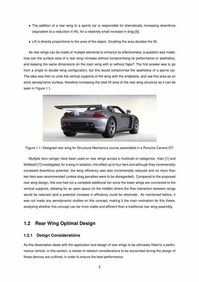
• The addition of a rear wing to a sports car is responsible for dramatically increasing downforce

(equivalent to a reduction in lift), for a relatively small increase in drag [6];

• Lift is directly proportional to the area of the object. Doubling the area doubles the lift.

As rear wings can be made of multiple elements to enhance its effectiveness, a question was made:

how can the surface area of a rear wing increase without compromising its performance or aesthetics,

and keeping the same dimensions on the main wing with or without flaps? The first answer was to go

from a single to double wing configuration, but this would compromise the aesthetics of a sports car.

The idea was then to unite the vertical supports of the wing with the endplates, and use this area as an

extra aerodynamic surface, therefore increasing the total lift area of the rear wing structure as it can be

seen in Figure 1.1.

Figure 1.1: Designed rear wing for Structural Mechanics course assembled in a Porsche Carrera GT.

Multiple tiers (wings) have been used on rear wings across a multitude of categories. Katz [1] and

McBeath [7] investigated, for a wing in isolation, this effect up to four tiers and although they incrementally

increased downforce potential, the wing efficiency was also incrementally reduced and no more than

two tiers was recommended (unless drag penalties were to be disregarded). Compared to the proposed

rear wing design, this one had not a complete additional tier since the lower wings are connected to the

vertical supports, allowing for an open space (in the middle) where the flow interaction between wings

would be reduced (and a potential increase in efficiency could be obtained). As mentioned before, it

was not made any aerodynamic studies on this concept, making it the main motivation for this thesis,

analysing whether this concept can be more viable and efficient than a traditional rear wing assembly.

1.2 Rear Wing Optimal Design

1.2.1 Design Considerations

As this dissertation deals with the application and design of rear wings to be ultimately fitted to a perfor-

mance vehicle, in this section, a review of relevant considerations to be accounted during the design of

these devices are outlined, in order to ensure the best performance.

2

Wing/body Interaction

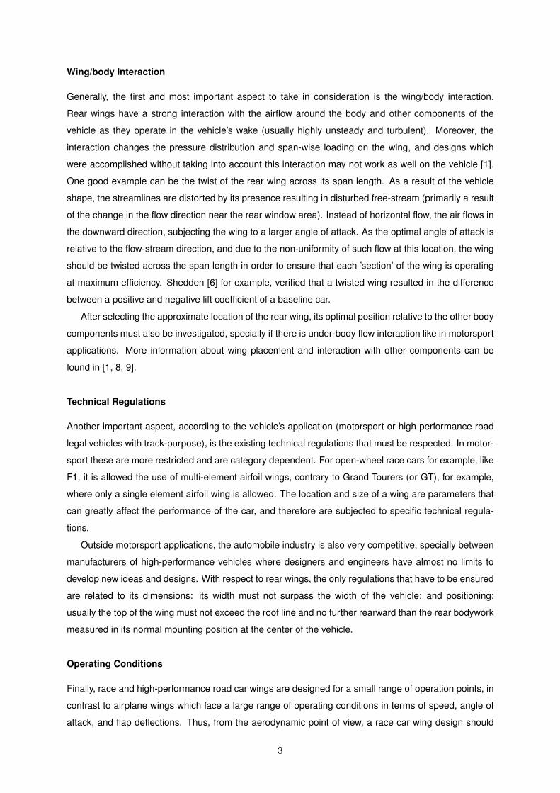
Generally, the first and most important aspect to take in consideration is the wing/body interaction.

Rear wings have a strong interaction with the airflow around the body and other components of the

vehicle as they operate in the vehicle’s wake (usually highly unsteady and turbulent). Moreover, the

interaction changes the pressure distribution and span-wise loading on the wing, and designs which

were accomplished without taking into account this interaction may not work as well on the vehicle [1].

One good example can be the twist of the rear wing across its span length. As a result of the vehicle

shape, the streamlines are distorted by its presence resulting in disturbed free-stream (primarily a result

of the change in the flow direction near the rear window area). Instead of horizontal flow, the air flows in

the downward direction, subjecting the wing to a larger angle of attack. As the optimal angle of attack is

relative to the flow-stream direction, and due to the non-uniformity of such flow at this location, the wing

should be twisted across the span length in order to ensure that each ’section’ of the wing is operating

at maximum efficiency. Shedden [6] for example, verified that a twisted wing resulted in the difference

between a positive and negative lift coefficient of a baseline car.

After selecting the approximate location of the rear wing, its optimal position relative to the other body

components must also be investigated, specially if there is under-body flow interaction like in motorsport

applications. More information about wing placement and interaction with other components can be

found in [1, 8, 9].

Technical Regulations

Another important aspect, according to the vehicle’s application (motorsport or high-performance road

legal vehicles with track-purpose), is the existing technical regulations that must be respected. In motor-

sport these are more restricted and are category dependent. For open-wheel race cars for example, like

F1, it is allowed the use of multi-element airfoil wings, contrary to Grand Tourers (or GT), for example,

where only a single element airfoil wing is allowed. The location and size of a wing are parameters that

can greatly affect the performance of the car, and therefore are subjected to specific technical regula-

tions.

Outside motorsport applications, the automobile industry is also very competitive, specially between

manufacturers of high-performance vehicles where designers and engineers have almost no limits to

develop new ideas and designs. With respect to rear wings, the only regulations that have to be ensured

are related to its dimensions: its width must not surpass the width of the vehicle; and positioning:

usually the top of the wing must not exceed the roof line and no further rearward than the rear bodywork

measured in its normal mounting position at the center of the vehicle.

Operating Conditions

Finally, race and high-performance road car wings are designed for a small range of operation points, in

contrast to airplane wings which face a large range of operating conditions in terms of speed, angle of

attack, and flap deflections. Thus, from the aerodynamic point of view, a race car wing design should

3

be easier to accomplish. Additionally, Reynolds number effects only become essential in race and road

car aerodynamics when significant speed variations exist along a certain track or when small-scale wind

tunnel tests are used to simulate the flow field of the actual vehicle. Nonetheless, nowadays the assem-

bly of a car rear wing allows the fine tuning of the angle of attack according to the track characteristics.

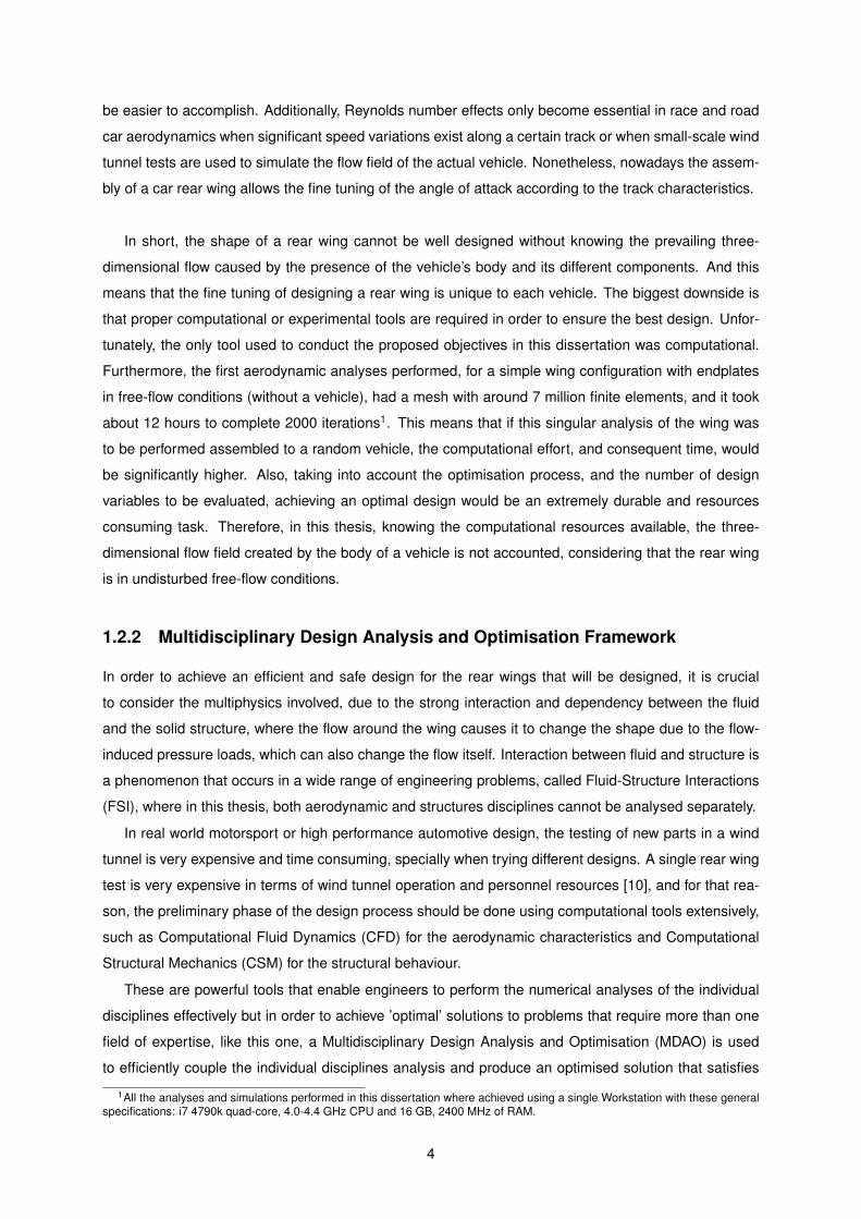
In short, the shape of a rear wing cannot be well designed without knowing the prevailing three-

dimensional flow caused by the presence of the vehicle’s body and its different components. And this

means that the fine tuning of designing a rear wing is unique to each vehicle. The biggest downside is

that proper computational or experimental tools are required in order to ensure the best design. Unfor-

tunately, the only tool used to conduct the proposed objectives in this dissertation was computational.

Furthermore, the first aerodynamic analyses performed, for a simple wing configuration with endplates

in free-flow conditions (without a vehicle), had a mesh with around 7 million finite elements, and it took

about 12 hours to complete 2000 iterations1. This means that if this singular analysis of the wing was

to be performed assembled to a random vehicle, the computational effort, and consequent time, would

be significantly higher. Also, taking into account the optimisation process, and the number of design

variables to be evaluated, achieving an optimal design would be an extremely durable and resources

consuming task. Therefore, in this thesis, knowing the computational resources available, the three-

dimensional flow field created by the body of a vehicle is not accounted, considering that the rear wing

is in undisturbed free-flow conditions.

1.2.2 Multidisciplinary Design Analysis and Optimisation Framework

In order to achieve an efficient and safe design for the rear wings that will be designed, it is crucial

to consider the multiphysics involved, due to the strong interaction and dependency between the fluid

and the solid structure, where the flow around the wing causes it to change the shape due to the flow-

induced pressure loads, which can also change the flow itself. Interaction between fluid and structure is

a phenomenon that occurs in a wide range of engineering problems, called Fluid-Structure Interactions

(FSI), where in this thesis, both aerodynamic and structures disciplines cannot be analysed separately.

In real world motorsport or high performance automotive design, the testing of new parts in a wind

tunnel is very expensive and time consuming, specially when trying different designs. A single rear wing

test is very expensive in terms of wind tunnel operation and personnel resources [10], and for that rea-

son, the preliminary phase of the design process should be done using computational tools extensively,

such as Computational Fluid Dynamics (CFD) for the aerodynamic characteristics and Computational

Structural Mechanics (CSM) for the structural behaviour.

These are powerful tools that enable engineers to perform the numerical analyses of the individual

disciplines effectively but in order to achieve ’optimal’ solutions to problems that require more than one

field of expertise, like this one, a Multidisciplinary Design Analysis and Optimisation (MDAO) is used

to efficiently couple the individual disciplines analysis and produce an optimised solution that satisfies

1All the analyses and simulations performed in this dissertation where achieved using a single Workstation with these generalspecifications: i7 4790k quad-core, 4.0-4.4 GHz CPU and 16 GB, 2400 MHz of RAM.

4

both of them. Coupling the aerodynamic and structural disciplines together defines the basic aero-

structural optimisation problem, and the tight relation between them, makes rear wing design suitable to

the application of MDAO methodologies.

Besides establishing the disciplines involved in the MDAO problem, in order to achieve an optimised

design of a rear wing, design variables and interest functions or objectives must be defined, which

requires proper geometric parametrisation. A Computer-Aided Design (CAD) tool, for example, incorpo-

rates parametric modelling capabilities and therefore allow designers and engineers to capture design

intents more effectively. Finally, after establishing the MDAO design variables and functions of inter-

est within the aerodynamic and structural disciplines, proper numerical optimisation method is required

to achieve the optimised design. This will be a subject of interest discussed during the course of this

dissertation. Figure 1.2 describes the overall scheme of the MDAO architecture established for the

aero-structural optimisation problem of this thesis.

Figure 1.2: MDAO framework established for the aero-structural optimisation problem.

1.3 Thesis Objectives

The main goal of this work is the design of a conventional rear wing and re-design of a custom rear

wing, including shape optimisation and optimal composite structure laminate layup, for a specific set

of requirements in terms of aerodynamic and structural responses and ultimately compare their perfor-

mances. The expect outcome is to fold the implementation of a process for optimal automotive aerody-

namic devices design.

The design will take into account both aerodynamic and structural disciplines and in particular the

interaction between them. The design will comprise several steps:

5

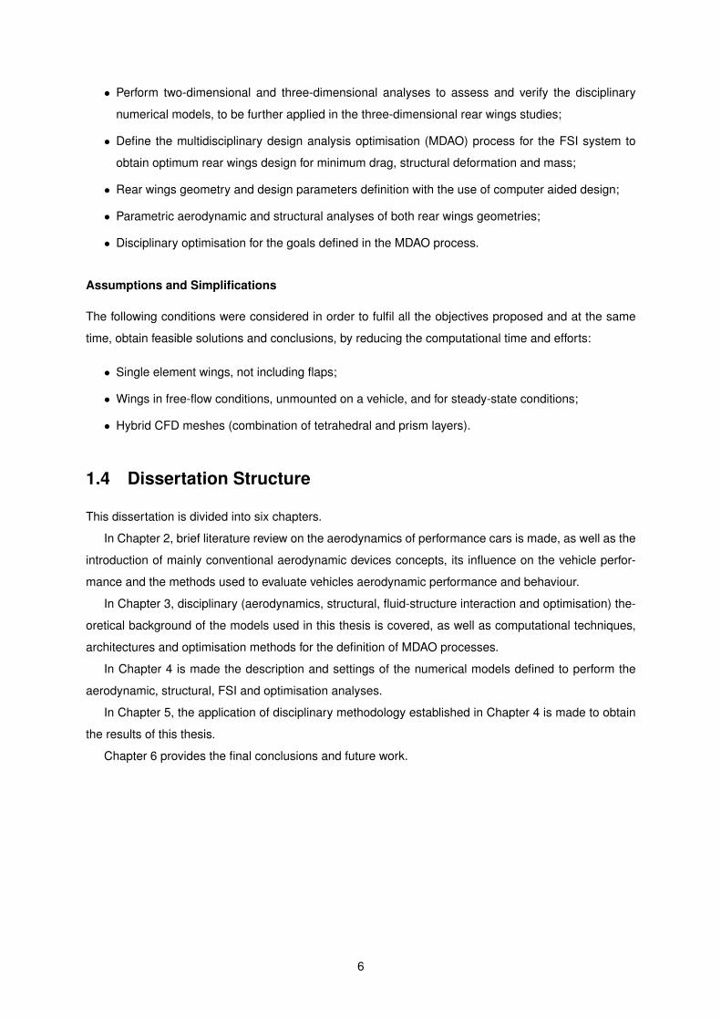
• Perform two-dimensional and three-dimensional analyses to assess and verify the disciplinary

numerical models, to be further applied in the three-dimensional rear wings studies;

• Define the multidisciplinary design analysis optimisation (MDAO) process for the FSI system to

obtain optimum rear wings design for minimum drag, structural deformation and mass;

• Rear wings geometry and design parameters definition with the use of computer aided design;

• Parametric aerodynamic and structural analyses of both rear wings geometries;

• Disciplinary optimisation for the goals defined in the MDAO process.

Assumptions and Simplifications

The following conditions were considered in order to fulfil all the objectives proposed and at the same

time, obtain feasible solutions and conclusions, by reducing the computational time and efforts:

• Single element wings, not including flaps;

• Wings in free-flow conditions, unmounted on a vehicle, and for steady-state conditions;

• Hybrid CFD meshes (combination of tetrahedral and prism layers).

1.4 Dissertation Structure

This dissertation is divided into six chapters.

In Chapter 2, brief literature review on the aerodynamics of performance cars is made, as well as the

introduction of mainly conventional aerodynamic devices concepts, its influence on the vehicle perfor-

mance and the methods used to evaluate vehicles aerodynamic performance and behaviour.

In Chapter 3, disciplinary (aerodynamics, structural, fluid-structure interaction and optimisation) the-

oretical background of the models used in this thesis is covered, as well as computational techniques,

architectures and optimisation methods for the definition of MDAO processes.

In Chapter 4 is made the description and settings of the numerical models defined to perform the

aerodynamic, structural, FSI and optimisation analyses.

In Chapter 5, the application of disciplinary methodology established in Chapter 4 is made to obtain

the results of this thesis.

Chapter 6 provides the final conclusions and future work.

6

Chapter 2

Automotive Aerodynamics

2.1 History of Aerodynamics in Performance Cars Design

Air resistance was the first major obstacle to automotive speed and fuel saving since the dawn of the

automobile. There was nothing aerodynamic about the earliest cars, but with the first races between

constructors, fast circuits with low power engines made engineers realise how much the frictional force

of aerodynamic drag increases significantly with the vehicle speed [11]. Thus, in the 1910s engineers

began to consider automobile shape in reducing aerodynamic drag at higher speeds incorporating ta-

pering features to the back-end of their cars. During the 1920s until the 1940s, adaptation from the

aeronautical industry resulted into tear-drop and slippery streamlined shaped cars.

Over the 1950s and 1960s , some of the biggest advancements in automobile aerodynamics came

from the F1 World Championship started in 1950, and the implementation of the organised World Sports

Car Championship (1953) regulated by the International Automobile Federation (FIA - Federation Inter-

nationale de l’Automobile). The typical sports prototype racing car of the 1950s was small, light weight,

front-engined and race car designers focused in making the most slippery aerodynamic body shapes

possible (round and streamlined) due to relative inefficient engines that lacked horsepower [12].

It was in the 1960s that motorsport teams started using reversed wings and the research for the

exploitation of downforce truly began. Tire and engines technology were also improved [11], focusing

teams in crafting the most aerodynamic race car possible. Front and rear cable operated spoilers and

wings to adjust the angle of attack, front air dams, fender vents, naturally aspirated mid-engine layouts

and shovel-shaped noses as well as aero-kits became more and more common to keep air flowing over

the body of the car and create fundamental downforce on the front and rear wheels [13].

These early experiments with high mountings adjustable wings, as well as high horsepower racing

engines led to many accidents, and by the early 1970s, frequent changes in regulations were presented

by the FIA. Because of them, this period lacked some of the excitement and innovation of past eras, but,

by the late 1970s, revolutionary advances in engines and aerodynamics were introduced in F1 racing.

Significant innovation was introduced in 1977 by the Lotus F1 team making use of the aerodynamic effect

that the lift of a wing increases with decreasing ground proximity, called ’ground effect ’. Their Lotus 78’s

7

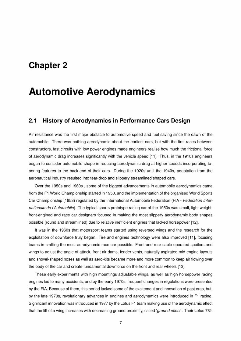
(Figure 2.1) side-pods were shaped like upside down wings creating tremendous amounts of downforce

underneath the car for a very little drag penalty, which boosted cornering speeds tremendously [12, 13].

(a) 1977 Lotus 78 ’wingcar ’. (b) 1977 Lotus 78 sidepods.

Figure 2.1: Introduction of ground effect by F1 Lotus team in 1977 [11].

The early 1980s marked the beginning of composite materials use. The McLaren F1 team introduced

carbon fibre and kevlar in the construction of the chassis, wings and body work that made prototype and

F1 cars lighter and stronger. All these elements, coupled with the continued development of ground

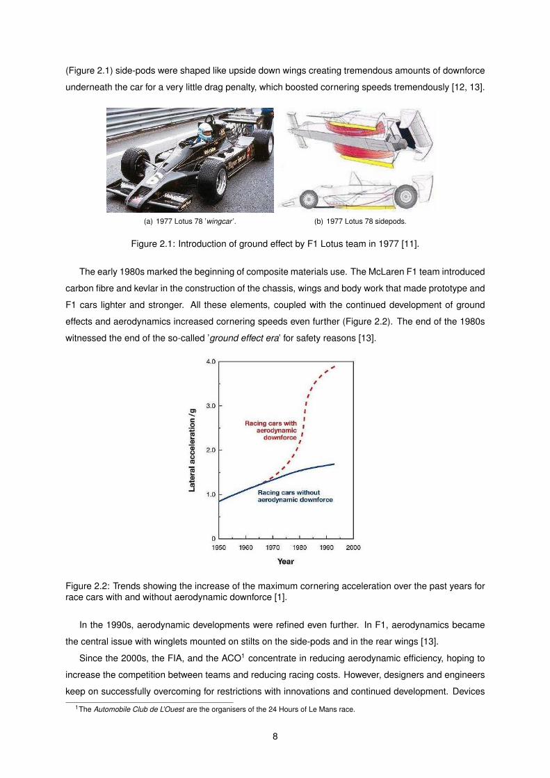
effects and aerodynamics increased cornering speeds even further (Figure 2.2). The end of the 1980s

witnessed the end of the so-called ’ground effect era’ for safety reasons [13].

Figure 2.2: Trends showing the increase of the maximum cornering acceleration over the past years for

race cars with and without aerodynamic downforce [1].

In the 1990s, aerodynamic developments were refined even further. In F1, aerodynamics became

the central issue with winglets mounted on stilts on the side-pods and in the rear wings [13].

Since the 2000s, the FIA, and the ACO1 concentrate in reducing aerodynamic efficiency, hoping to

increase the competition between teams and reducing racing costs. However, designers and engineers

keep on successfully overcoming for restrictions with innovations and continued development. Devices

1The Automobile Club de L’Ouest are the organisers of the 24 Hours of Le Mans race.

8

such as double rear diffusers, F-ducts, and exhaust-blown diffusers were introduced and quickly banned,

but their ingenuity means that every now and then, a loophole will be found in the regulations and a clever

aerodynamic solution will be introduced.

2.1.1 The Impact of Motorsport Aerodynamics on Production Cars

Aerodynamics in production passenger cars is crucial as the air resistance is the primary concern for

passenger car aerodynamicists. It influences driving performance and stability, fuel consumption, ac-

celeration and top speed [13]. The influence of motorsport is undeniable, and passenger cars greatly

benefit from these technological advances. There is also another class of road-legal vehicles that take

full advantage of racing. High-powered engines, ultra-light construction using advanced composite mate-

rials, low drag and high downforce makes this road-legal cars the closest to performance racing vehicles,

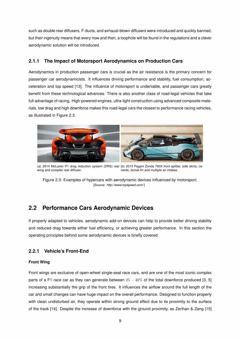
as illustrated in Figure 2.3.

(a) 2014 McLaren P1 drag reduction system (DRS) rearwing and complex rear diffuser.

(b) 2015 Pagani Zonda 760X front splitter, side skirts, ca-nards, dorsal fin and multiple air intakes.

Figure 2.3: Examples of hypercars with aerodynamic devices influenced by motorsport.

[Source: http://www.topspeed.com/ ]

2.2 Performance Cars Aerodynamic Devices

If properly adapted to vehicles, aerodynamic add-on devices can help to provide better driving stability

and reduced drag towards either fuel efficiency, or achieving greater performance. In this section the

operating principles behind some aerodynamic devices is briefly covered.

2.2.1 Vehicle’s Front-End

Front Wing

Front wings are exclusive of open-wheel single-seat race cars, and are one of the most iconic complex

parts of a F1 race car as they can generate between 25 − 40% of the total downforce produced [3, 5]

increasing substantially the grip of the front tires. It influences the airflow around the full length of the

car and small changes can have huge impact on the overall performance. Designed to function properly

with clean undisturbed air, they operate within strong ground effect due to its proximity to the surface

of the track [14]. Despite the increase of downforce with the ground proximity, as Zerihan & Zang [15]

9

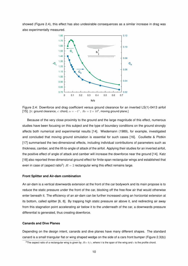
showed (Figure 2.4), this effect has also undesirable consequences as a similar increase in drag was

also experimentally measured.

Figure 2.4: Downforce and drag coefficient versus ground clearance for an inverted LS(1)-0413 airfoil

[15]. [h: ground clearance, c: chord, α = −1◦ , Re = 2× 10

6, moving ground plane.]

Because of the very close proximity to the ground and the large magnitude of this effect, numerous

studies have been focusing on this subject and the type of boundary conditions on the ground strongly

affects both numerical and experimental results [14]. Wiedemann (1989), for example, investigated

and concluded that moving ground simulation is essential for such cases [16]. Coulliette & Plotkin

[17] summarised the two-dimensional effects, including individual contributions of parameters such as

thickness, camber, and the lift-to-angle of attack of the airfoil. Applying their studies for an inverted airfoil,

the positive effect of angle of attack and camber will increase the downforce near the ground [14]. Katz

[18] also reported three-dimensional ground effect for finite-span rectangular wings and established that

even in case of (aspect ratio2)A = 2 rectangular wing this effect remains large.

Front Splitter and Air-dam combination

An air-dam is a vertical downwards extension at the front of the car bodywork and its main propose is to

reduce the static pressure under the front of the car, blocking off the free-flow air that would otherwise

enter beneath it. The efficiency of an air-dam can be further increased using an horizontal extension at

its bottom, called splitter [6, 8]. By trapping high static pressure air above it, and redirecting air away

from this stagnation point accelerating air below it to the underneath of the car, a downwards pressure

differential is generated, thus creating downforce.

Canards and Dive Planes

Depending on the design intent, canards and dive planes have many different shapes. The standard

canard is a small triangular flat or wing shaped wedge on the side of a cars front bumper (Figure 2.3(b))

2The aspect ratio of a rectangular wing is given byA= b/c, where b is the span of the wing and c is the profile chord.

10

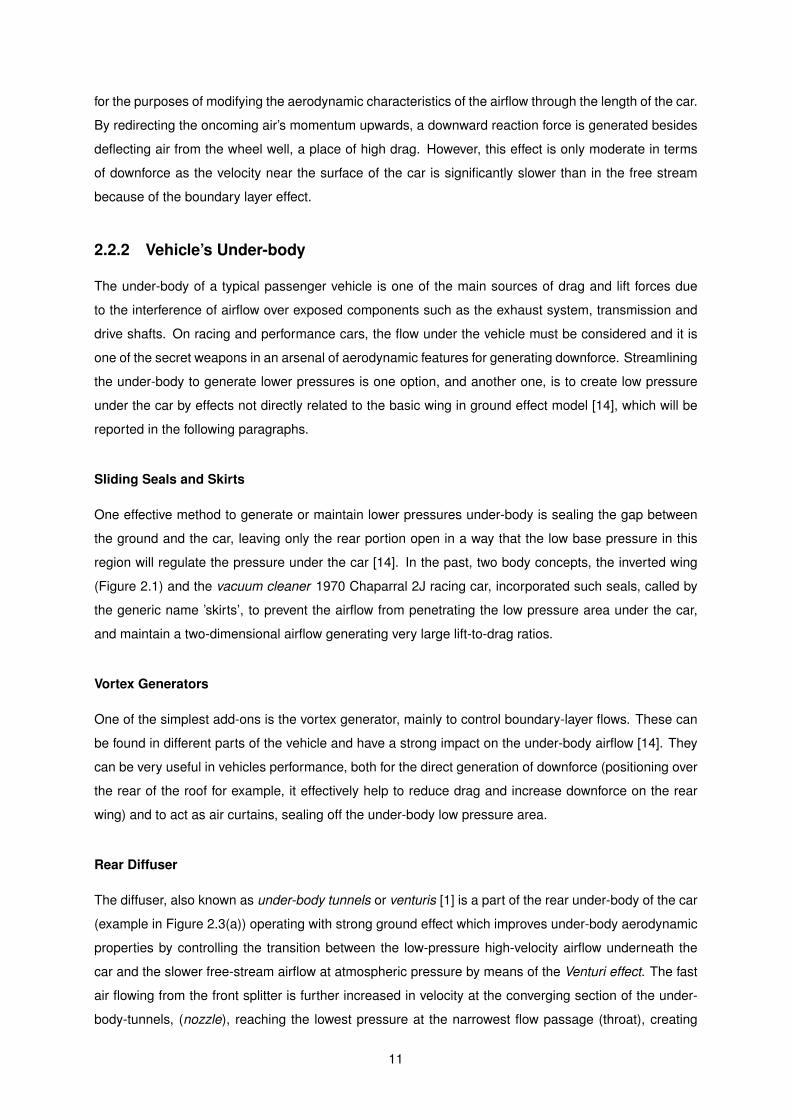
for the purposes of modifying the aerodynamic characteristics of the airflow through the length of the car.

By redirecting the oncoming air’s momentum upwards, a downward reaction force is generated besides

deflecting air from the wheel well, a place of high drag. However, this effect is only moderate in terms

of downforce as the velocity near the surface of the car is significantly slower than in the free stream

because of the boundary layer effect.

2.2.2 Vehicle’s Under-body

The under-body of a typical passenger vehicle is one of the main sources of drag and lift forces due

to the interference of airflow over exposed components such as the exhaust system, transmission and

drive shafts. On racing and performance cars, the flow under the vehicle must be considered and it is

one of the secret weapons in an arsenal of aerodynamic features for generating downforce. Streamlining

the under-body to generate lower pressures is one option, and another one, is to create low pressure

under the car by effects not directly related to the basic wing in ground effect model [14], which will be

reported in the following paragraphs.

Sliding Seals and Skirts

One effective method to generate or maintain lower pressures under-body is sealing the gap between

the ground and the car, leaving only the rear portion open in a way that the low base pressure in this

region will regulate the pressure under the car [14]. In the past, two body concepts, the inverted wing

(Figure 2.1) and the vacuum cleaner 1970 Chaparral 2J racing car, incorporated such seals, called by

the generic name ’skirts’, to prevent the airflow from penetrating the low pressure area under the car,

and maintain a two-dimensional airflow generating very large lift-to-drag ratios.

Vortex Generators

One of the simplest add-ons is the vortex generator, mainly to control boundary-layer flows. These can

be found in different parts of the vehicle and have a strong impact on the under-body airflow [14]. They

can be very useful in vehicles performance, both for the direct generation of downforce (positioning over

the rear of the roof for example, it effectively help to reduce drag and increase downforce on the rear

wing) and to act as air curtains, sealing off the under-body low pressure area.

Rear Diffuser

The diffuser, also known as under-body tunnels or venturis [1] is a part of the rear under-body of the car

(example in Figure 2.3(a)) operating with strong ground effect which improves under-body aerodynamic

properties by controlling the transition between the low-pressure high-velocity airflow underneath the

car and the slower free-stream airflow at atmospheric pressure by means of the Venturi effect. The fast

air flowing from the front splitter is further increased in velocity at the converging section of the under-

body-tunnels, (nozzle), reaching the lowest pressure at the narrowest flow passage (throat), creating

11

substantially amounts of downforce [1]. The diverging section (diffuser) aims to decelerate the airflow

and increase static pressure to ambient conditions in order to correctly recover the kinetic energy of

the airflow under the car as efficiently as possible, and therefore reduce drag. If properly designed, a

diffuser is a very effective aerodynamic device and in a modern F1 car, for example, the diffuser alone

can produce up to 40% of the total downforce [5].

2.2.3 Vehicle’s Back-End

Spoiler

Commonly interchanged with wings, spoilers are obstructions to undesirable airflow behaviour around

the vehicle and can be found in almost every type of vehicles. Usually they are mounted either on the

front (called air-dams and covered in Subsection 2.2.1) or at the rear deck. Their main goal is to reduce

drag and improve fuel efficiency [1]. On passenger vehicles, especially hatchbacks, the adverse pres-

sure gradients created by the steep angle from the roof to the rear window contributes to the separation

of the airflow in this area, generating wake turbulence (pushing the car up and down) that causes driving

instability at high speeds and adds a lot of drag. By incorporating such devices in this region, airflow

separation is delayed minimising turbulence (reducing drag) and improving fuel efficiency. Sharma &

Bansal [19] performed a CFD simulation for the flow over a passenger car incorporating such devices

measuring a 3.87% reduction in the CD and 16.62% reduction in the CL, aiding the stability and fuel

efficiency of passenger cars.

Rear Wing

Rear wings can be found on high-performance road legal vehicles (example Figure 2.3) as well as in

almost every type of racing vehicles. They generate essential downforce to increase back wheels traction

thus reducing rear axle lift (improving cornering speeds and high-speed braking), at the cost of adding

high drag values, which places severe limits on the top speed of the car. In contrast to front wings, as

mentioned in Subsection 1.2.1, rear wings operate in the vehicle’s wake (usually highly unsteady and

turbulent) [14, 20]. Katz & Largman [21] performed experimental studies of an enclosed wheel race

car with and without a rear wing (Figure 2.5) and stated that the aerodynamic downforce ’is strongly

affected by the interaction between the rear wing and the flow beneath the vehicle’. Later, Katz &

Dykstra [22] investigated the influence of rear-mount wings on the aerodynamics of two generic race car

configurations and concluded that the downforce levels are larger with the coupled configuration than the

combined contribution of the wing and the vehicle alone, and that its interaction also alters the pressure

distribution and span-wise loading on the wing. Therefore, the three-dimensional flow field created by

the body should always be taken into account in the design process of rear wings, and its placement (in

the absence of beneficial under-body interaction) should be as high as possible so that little disturbed

airflow reaches the wing, maximising downforce [1, 9, 23, 7].

Apart from the vehicle and rear wing interaction, there are another ways to improve its efficiency, such

as the use of gurney flaps and endplates. The gurney flap is a short flat plate attached to the trailing

12

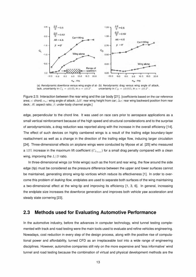
(a) Aerodynamic downforce versus wing angle of at-tack, uncertainty in CL = ±0.03, in α = ±0.2◦ .

(b) Aerodynamic drag versus wing angle of attack,uncertainty in CD = ±0.015, in α = ±0.2◦ .

Figure 2.5: Interaction between the rear wing and the car body [21]. [coefficients based on the car reference

area; c: chord; αw: wing angle of attack; ∆H: rear wing height from car; ∆x: rear wing backward position from rear

deck;A: aspect ratio; β: under-body channel angle.]

edge, perpendicular to the chord line. It was used on race cars prior to aerospace applications as a

small vertical reinforcement because of the high speed and structural considerations and to the surprise

of aerodynamicists, a drag reduction was reported along with the increase in the overall efficiency [14].

The effect of such devices on highly cambered wings is a result of the trailing edge boundary-layer

reattachment as well as a change in the direction of the trailing edge flow, inducing larger circulation

[24]. Three-dimensional effects on airplane wings were conducted by Myose et al. [25] who measured

a 13% increase in the maximum lift coefficient (CLmax) for a small drag penalty compared with a clean

wing, improving the L/D ratio.

In three-dimensional wings (or finite wings) such as the front and rear wing, the flow around the side

edge (tip) must be considered as the pressure difference between the upper and lower surfaces cannot

be maintained, generating strong wing-tip vortices which reduce its effectiveness [1]. In order to over-

come this problem of leaking flow, endplates are used to separate both surfaces of the wing maintaining

a two-dimensional effect at the wing-tip and improving its efficiency [1, 3, 6]. In general, increasing

the endplate size increases the downforce generation and improves both vehicle yaw acceleration and

steady state cornering [23].

2.3 Methods used for Evaluating Automotive Performance

In the automotive industry, before the advances in computer technology, wind tunnel testing comple-

mented with track and road testing were the main tools used to evaluate and refine vehicles engineering.

Nowadays, cost reduction in every step of the design process, along with the positive rise of computa-

tional power and affordability, turned CFD as an irreplaceable tool into a wide range of engineering

disciplines. However, automotive companies still rely on the more expensive and ’less informative’ wind

tunnel and road testing because the combination of virtual and physical development methods are the

13

most reliable way to effectively improve a vehicle performance.

2.3.1 Numerical Simulations

CFD is a modern computational analysis tool that provides numerical solutions using algorithms to

solve fluid flow governing equations (Navier-Stokes equations), in order to simulate determined physi-

cal conditions. Motorsport was one of the first professional sports to adopt commercial CFD tools for

competitive advantage because of its relative cheapness and scalable knowledge, relative to building

further wind tunnels. Besides the increase of computational power over the last two decades, the other

biggest influence on the CFD market has been the growth of CAD tools, which enabled complex real-

world geometries to be created and parametrised [26]. Combining both CAD and CFD tools, engineers

could quickly evaluate and develop new design ideas without the requirement of costly prototype testing.

However, such instrument has its own weaknesses. It is only a simulation of what could happen in the

real world, and the numerical solution strongly depends on user-defined elements (mesh generation

and turbulence modelling). Such modelling techniques have an important effect on the quality of the

numerical solution, in particular for the prediction of flow separation (in smooth curved surfaces) and for

the transition from laminar to turbulent flow at high-Reynolds numbers [14].

One example of the research of such user-defined elements influence are the American Institute

of Aeronautics and Astronautics (AIAA) CFD Drag Prediction Workshops. They have been comparing

several solutions methods with wind tunnel results for the flow over generic airplanes configurations, spe-

cially the prediction of the incremental drag associated with the nacelle/pylon installation [27, 28, 29].

In general, the conclusion is that the grid attributes (quality and resolution) and turbulence modelling

choice have a crucial affect in the results of the force coefficients, due to differences both in friction drag

and predicted flow phenomena, such as the large separation zone at the wing-body junction. Although

achieving good comparison with experiment results, in general the estimation of lift is more accurate

(although over-predicted) than that of the drag force (usually under-predicted). Same results were ob-

tained by Wordley & Saunders [23] for example. Such conclusions are as well very relevant to the

high-Reynolds number flow over race cars, dominated by both laminar and turbulent flow regimes and

localised flow separations.

2.3.2 Wind Tunnel Testing

As the capability of a CFD simulation to predict flow behaviour depends on the modelling techniques

utilised, it is very important to validate and correlate CFD results with physical experimentation. This

can be achieved through road or track testing, however, a safer and more convenient alternative is the

use of scale model wind tunnel testing. Besides the cost reduction, such facilities provides a controlled

test environment isolated from external weather effects.

Wind tunnel methodology became an essential tool in the race car design during the 1960s, when

the significance of aerodynamics was realised (Section 2.1). At this time, such methods were already

advanced and widely used by the aerospace industry, but such facilities imposed several difficulties for

14

the testing of race cars. The major problems was due to the small clearance between the vehicle under-

body and the stationary floor of the test section and the mounting of the rotating wheels [14]. These are

very important measures to take in account when testing vehicles performance and the moving ground

simulation is essential for such cases [16]. Solutions to simulate the moving ground simulation were

reported by Katz [1], in the form of blowing, suction, rolling grounds, symmetry or all of them combined,

along with techniques for the mounting of rotating wheels.

Through the 1980s and 1990s customised wind tunnel facilities were rapidly increasing and devel-

oped for general automotive and race car testing, all with moving ground simulation [1]. In order to

avoid or minimise effects of blockage and boundary layer generation, working section area, model size

and correct Reynolds number must be carefully selected to accurately predict aerodynamic behaviour

of full-size models.

2.3.3 Road and Track Testing

Comparing both experimental methodologies used to evaluate aerodynamic performance of vehicles,

the difficulties associated with wind tunnel testing: moving ground, rolling wheels, the correct Reynolds

number and wind tunnel blockage correction, are all resolved on the full-scale testing on the road or race

track. Although the vehicle must exists, be more expensive (track renting if not owned by manufacturers

and instrumentation) and dependent on the weather conditions, with the advance in sensor technology

and data acquisition systems, desirable forces, moments and pressures can be easily measured, trans-

mitted via wireless communication and analysed in real time [14]. If the external conditions cooperate,

this is ultimately the most accurate way to evaluate the vehicles performance and to validate CFD or

wind tunnel results.

15

Chapter 3

Theoretical Background

In this chapter, Fluid-Structure Interaction is discussed, mainly the types of approach that can be utilised

to solve multiphysics problems. FSI is a combination of fluid and structural dynamics, so it is essential

to understand the basic physical principles and governing equations of fluid flow and thin structures

(particular of rear wings), which can both be described by the relations of continuum mechanics and

mostly solved with numerical methods. Besides the aerodynamic and thin structures fundamental theory,

the Multidisciplinary Design Analysis and Optimisation architectures will be briefly reviewed along with

some numerical optimisation methods commonly used.

3.1 Aerodynamic Theory

In Section 2.3.1, CFD was introduced, covering its advantages as well as the principal concerns when

performing numerical simulations to predict the flow behaviour of physical problems. Such concerns,

referred as user-defined elements, are related with the numerical grid generation and turbulence mod-

elling that have a crucial effect on the quality of the numerical solution, which were investigated in the

following Chapter 4.

3.1.1 Governing Equations of Fluid Flow

The time dependent three-dimensional fluid flow and heat transfer around a body consist of the conti-

nuity equation (conservation of mass), momentum equations (conservation of momentum) and energy

equation (conservation of energy) [20].

The general approach in automotive external aerodynamics is to assume incompressible flow (the

air density is constant and is considered as an ideal gas1), and isothermal flow (constant temperature)

[8, 20]. The flow can be considered incompressible when the Mach number2, M , is under 0.3. In

automotive aerodynamics, it is unlikely that such speeds will be achieved and so compressibility effects

1The ideal gas law is the equation of state of a hypothetical ideal gas and can be written as p = ρRT , where p is the pressure,ρ is the density R is universal gas constant (for air R ≈ 287J kg−1 K−1) and T is the temperature.

2Mach number is a dimensionless quantity representing the ratio of the body velocity u to the local speed of sound c: M = u

c

17

can be disregarded [1, 8, 20]. Thus, the energy equation can be neglected and the continuity and

momentum equations can be written on the incompressible form [20] respectively, as

∂u

∂x+

∂v

∂y+

∂w

∂z= 0 , (3.1)

ρDu

Dt= ρgx −

∂p

∂x+ µ

(

∂2u

∂x2+

∂2u

∂y2+

∂2u

∂z2

)

,

ρDv

Dt= ρgy −

∂p

∂y+ µ

(

∂2v

∂x2+

∂2v

∂y2+

∂2v

∂z2

)

,

ρDw

Dt= ρgz −

∂p

∂z+ µ

(

∂2w

∂x2+

∂2w

∂y2+

∂2w

∂z2

)

,

(3.2)

where ρ is the fluid density, u, v and w are the components of the fluid velocity, g represents the body

accelerations (per unit mass) acting on the continuum (gravity and/or inertial accelerations), p is the fluid

pressure, µ is the fluid dynamic viscosity and DDt

≡ ∂∂t

+ u ∂∂x

+ v ∂∂y

+ w ∂∂z

.

It is important to recall that the momentum equations (3.2) are the application of Newton’s second

law of motion to fluid flow. The left-hand side of these equations represents the total rate of change

of momentum per unit volume and the three terms on the right-hand side represent the body force,

pressure and viscous forces, respectively, acting on a unit volume of fluid. This form of the momentum

equations (3.2) is known as the Incompressible Flow Navier-Stokes equations [20]. They are second

order non-linear partial differential equations and are solved for a finite number of control-volumes which

are referred to as a computational grid (or mesh). Most commercial CFD codes use the finite-volume

method for the discretisation of such equations with at least second-order accuracy. Detailed information

on the finite-volume discretisation can be found in [30, 31].

3.1.2 Turbulent Flows and Turbulence Modelling

Turbulence has to be one of the most challenging areas in fluid dynamics and a very important limiting

factor in accurate computer simulation of engineering flows. According to Menter (developer of the

widely used Shear-Stress Transport (SST) turbulence model), the ’turbulence modelling is the attempt to

develop approximate formulations that, despite our incomplete understanding and limited computational

resources, allow engineers to obtain approximate solutions for their technological applications’ [32].

Reynolds Averaged Navier-Stokes

An averaging concept for the Navier-Stokes equations was proposed by Reynolds, that significantly

reduces the complexity of simulating turbulent flows [32]. The resulting Reynolds-averaged Navier-

Stokes (RANS) equations are formulated in terms of the time-averaged flow field (velocity field and

pressure for incompressible isothermal flow). For example the time-averaged of the turbulent velocity

function in the x-direction is given by

u =1

T

∫ t0+T

t0

u dt , (3.3)

18

and all instantaneous properties are split into a mean and fluctuation component as

u = u+ u′ , v = v + v′ , w = w + w′ , p = p+ p′ . (3.4)

When these properties from Equations (3.4) are replaced by its mean and fluctuation components, and

time averaging is taken, the three dimensional continuity and RANS equations are formed and can be

expressed as [33]:∂u

∂x+

∂v

∂y+

∂w

∂z= 0 , (3.5)

ρDu

Dt= ρgx −

∂p

∂x+

∂

∂x

(

µ∂u

∂x− ρu′u′

)

+∂

∂y

(

µ∂u

∂y− ρu′v′

)

+∂

∂z

(

µ∂u

∂z− ρu′w′

)

,

ρDv

Dt= ρgy −

∂p

∂y+

∂

∂x

(

µ∂v

∂x− ρu′v′

)

+∂

∂y

(

µ∂v

∂y− ρv′v′

)

+∂

∂z

(

µ∂v

∂z− ρv′w′

)

,

ρDw

Dt= ρgz −

∂p

∂z+

∂

∂x

(

µ∂w

∂x− ρu′w′

)

+∂

∂y

(

µ∂w

∂y− ρv′w′

)

+∂

∂z

(

µ∂w

∂z− ρw′w′

)

.

(3.6)

Although this process eliminates turbulence fluctuations, the price for this simplification lies in additional

Reynolds stress tensors (ρuiuj) in the RANS equations, as a result of the non-linear terms from the

underlying Navier-Stokes equations [33].

Turbulent near-wall treatment

Turbulent flows are significantly affected by the presence of walls. The no-slip condition at the wall must

be satisfied and a boundary layer is generated. The boundary layer is the layer of fluid in the immediate

vicinity of the wall where the effects of viscosity are significant. Numerous experiments have shown that

the near-wall region can be subdivided into three regions [31, 33]. The region in contact with the wall

is called viscous sublayer where the flow is almost laminar and the viscous effects play a dominant role

in momentum and heat or mass transfer [31]. In the outer layer, called the fully turbulent region (or log-

law region), turbulence plays a major role, and the in between region of the viscous sublayer and fully

turbulent layer is called buffer layer, where both molecular viscosity and turbulence effects cannot be

neglected. Fig. 3.1 illustrates these subdivisions of the near-wall region, plotted in semi-log coordinates.

More detailed information about these layers can be found in [33]. In the fluid flow direction, x-axis, the

dimensionless wall distance is defined as

y+ =y uτ

ν, (3.7)

where uτ is the friction velocity defined as√

τwρ

(τw is the wall shear stress), ν is fluid kinematic viscosity

and y is the height of the first cell.

The success of RANS models is essentially established by the efficiency and accuracy in the compu-

tation of wall-bounded flows. All turbulence models can virtually predict zero-gradient boundary layers,

but, for more complex shapes, with smooth surfaces under adverse pressure-gradients (like airfoils for

example) have resulted in the need for turbulence models that are able to predict flow separation and

transition from laminar to turbulent flow in a demand of high accuracy. Such accuracy requirements are

19

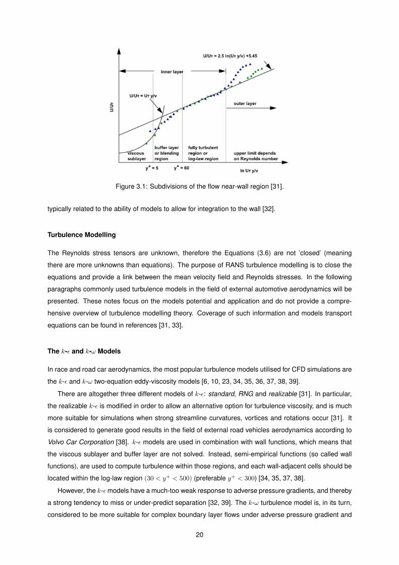
Figure 3.1: Subdivisions of the flow near-wall region [31].

typically related to the ability of models to allow for integration to the wall [32].

Turbulence Modelling

The Reynolds stress tensors are unknown, therefore the Equations (3.6) are not ’closed’ (meaning

there are more unknowns than equations). The purpose of RANS turbulence modelling is to close the

equations and provide a link between the mean velocity field and Reynolds stresses. In the following

paragraphs commonly used turbulence models in the field of external automotive aerodynamics will be

presented. These notes focus on the models potential and application and do not provide a compre-

hensive overview of turbulence modelling theory. Coverage of such information and models transport

equations can be found in references [31, 33].

The k-ǫ and k-ω Models

In race and road car aerodynamics, the most popular turbulence models utilised for CFD simulations are

the k-ǫ and k-ω two-equation eddy-viscosity models [6, 10, 23, 34, 35, 36, 37, 38, 39].

There are altogether three different models of k-ǫ: standard, RNG and realizable [31]. In particular,

the realizable k-ǫ is modified in order to allow an alternative option for turbulence viscosity, and is much

more suitable for simulations when strong streamline curvatures, vortices and rotations occur [31]. It

is considered to generate good results in the field of external road vehicles aerodynamics according to

Volvo Car Corporation [38]. k-ǫ models are used in combination with wall functions, which means that

the viscous sublayer and buffer layer are not solved. Instead, semi-empirical functions (so called wall

functions), are used to compute turbulence within those regions, and each wall-adjacent cells should be

located within the log-law region (30 < y+ < 500) (preferable y+ < 300) [34, 35, 37, 38].

However, the k-ǫ models have a much-too weak response to adverse pressure gradients, and thereby

a strong tendency to miss or under-predict separation [32, 39]. The k-ω turbulence model is, in its turn,

considered to be more suitable for complex boundary layer flows under adverse pressure gradient and

20

separation, as found in external aerodynamics [32, 37, 38]. It uses the near-wall formulation which

means that the near-wall region is solved all the way down to the viscous sublayer (y+ < 5) [32, 35, 38].

Nevertheless, according to Menter [32] the k-ω model has shown a ’disturbing sensitivity to freestream

values imposed for ω at the boundary layer edge’, which led to development of a formulation that com-

bines the best of the k-ǫ and k-ω models. The resulting k-ω SST (Shear-stress Transport) model [40]

uses a blending function to make it behave as a k-ω model in the near-wall region and as a k-ǫ model in

the far wake region [31].

The γ-Reθt (Transition SST) Model

One of the major drawbacks of the two-equation turbulence models is that they model the flow as fully

turbulent and do not predict separation points as accurately as is sometimes required. For the flow over

airfoils or wings, a result in using such models is the over-prediction of the drag [32]. To accurately

predict the onset of transition and describe both laminar and turbulent regimes, additional equations are

needed.

The γ-Reθt, or Transition SST model, solves two additional transport equations, one for the intermit-

tency γ to trigger the transition onset, which is based on experimental correlations, and another one for

the transition onset Reynolds number Reθt, to avoid additional non-local operations introduced by the

quantities used in the experimental correlations [32, 31], thus making it a four-equation model.

The γ-Reθt transition model has been validated for a wide range of experimental data and is success-

fully used today in many industrial CFD simulations, such as in turbomachinery blades, wind turbines,

design of sailing yachts and more importantly, in racing cars [32].

3.2 Structures Theory

Similar to fluid flow systems, solid mechanics physics is governed by the relations of continuum me-

chanics: conservation of mass, momentum and energy.

3.2.1 Governing Equations of Solid Structure

The calculations for the structure side are based on the impulse conservation [41], solved by a finite

element approach described as

M · ~u+C · ~u+K · ~u = ~F , (3.8)

where M is the global mass matrix, C the global damping matrix, K the global stiffness matrix, ~F is the

vector of external forces and ~u, ~u and ~u are the nodal acceleration, velocity and displacements vectors,

respectively. For static (no time-dependent) analysis this equation becomes simply K · ~u = ~F .

21

3.2.2 First-Order Deformation Theory

This thesis deals not only with isotropic linear elastic materials, governed by the generalised Hooke’s

law, but also with fibre-reinforced laminated anisothropic materials, such as carbon fibre, as mentioned

in Section 1.1. In the analysis of thin and layered composite structures, shell elements are widely used

to keep the computational effort reasonable [42] and in-plane stresses and transverse shear stresses

can be predicted with good accuracy using shells based on the First-Order Shear Deformation Theory

(FSDT), described by [4].

In the FSDT, the Kirchhoff hypothesis is relaxed as the transverse normals do not remain perpen-

dicular to the midsurface after deformation, which amounts to including transverse shear strains in the

theory. Under the same assumptions and restrictions as in the classical laminate theory, according to

the displacement field of the first-order theory is of the form

u(x, y, z, t) = u0(x, y, t) + zφx(x, y, t) ,

v(x, y, z, t) = v0(x, y, t) + zφy(x, y, t) ,

w(x, y, z, t) = w0(x, y, t) ,

(3.9)

where u0, v0 and w0 denote the displacements of a point on the plane z = 0 (middle plane), and φx = ∂u∂z

and φy = ∂v∂z

are the rotations of a transverse normal about the y and x axes, respectively. These

quantities are called generalised displacements. For thin plates, the rotation functions φx and φy should

approach the respective slopes of the transverse deflection: φx = −∂w0

∂xand φy = −∂w0

∂y. The non-linear

strains associated with the displacement field are (Equations (3.9)) obtained by:

εxx =∂u0

∂x+

1

2

(

∂w0

∂x

)2

+ z∂φx

∂x,

γxy =

(

∂u0

∂y+

∂v0∂x

+∂w0

∂x

∂w0

∂y

)

+ z

(

∂φx

∂y+

∂φy

∂x

)

,

εyy =∂v0∂y

+1

2

(

∂w0

∂y

)2

+ z∂φy

∂y,

γxz =∂w0

∂x+ φx , γyz =

∂w0

∂y+ φy , ǫzz = 0 .

(3.10)

The stresses relative to the x y axes are now determined from the strains, and this must take into

consideration that each ply will, in general, have a different stiffness depending on its own properties

and orientation with respect to the x y axes. This is accounted for by computing the transformed stiffness

matrix Q as described in [4]. The properties of each ply must be transformed into a common x y axes,

chosen arbitrarily for the entire laminate, and the stresses at any vertical position are given by σ = Q ε,

which can also be described as σ = Q ε0 + zQ k.

Similar to laminated beam analysis, the middle plane strains must be related to applied forces and

moments by static equilibrium. The complete set of relations between applied forces and moments (per

22

unit width), and the resulting middle plane strains, can be summarised as a single matrix equation [4]:

N

M

=

A B

B D

ǫ0

k

. (3.11)

Further detail about the extensional stiffness matrix A, coupling stiffness matrix B and bending stiffness

matrix D can be found in [4].

With the above relations, stresses and displacements in laminated composites subjected to in-plane

traction or bending loads for each material type in the stacking sequence can be determined. Also if

desired, the individual ply stresses can be used to assess its failure possibility. The Maximum Stress

criterion,

σ1

σ1

= 1 ,σ2

σ2

= 1 ,τ12τ12

= 1 , (3.12)

and the Tsai-Hill failure criterion,

(

σ1

σ2

)2

−σ1 σ2

σ21

+

(

σ2

σ2

)2

+

(

τ12τ12

)2

= 1 , (3.13)

are widely used for this purpose [43, 44]. Here, σ1 and σ2 are the maximum principal stresses along the

longitudinal and transverse fibre directions and σ1 and σ2 are the ply longitudinal and transverse tensile

strengths, respectively. τ12 is the maximum shear stress and τ12 is the intralaminar (shear) ply strength.

The prediction of failure by these criteria occurs whenever the left-hand-side of Equations (3.12) and

(3.13) equals or exceeds unity.

3.3 Fluid-Structure Interaction (FSI)

FSI is an important subset of multiphysics applications where there is an interface surface between the

solid and the fluid domain. At this fluid-solid interface, both governing equations and boundary condi-

tions from the fluid and solid domain must be satisfied simultaneously, and a set of coupling boundary

conditions are introduced to close the system of equations. Such coupling conditions can be classi-

fied as kinematic, which defines the motion and ensures the compatibility of displacement across the

fluid-solid interface and traction (dynamic) condition that satisfies the stress/force balance ensuring the

compatibility of traction across the fluid-solid interface [34, 41, 45]. Since this dissertation deals with an

aero-structural problem, and not aero-elastic, the only coupling condition to be satisfied at the interface

is the kinematic. According to Wang & Yan [45], it can be written as

dfΓ= dsΓ , (3.14)

23

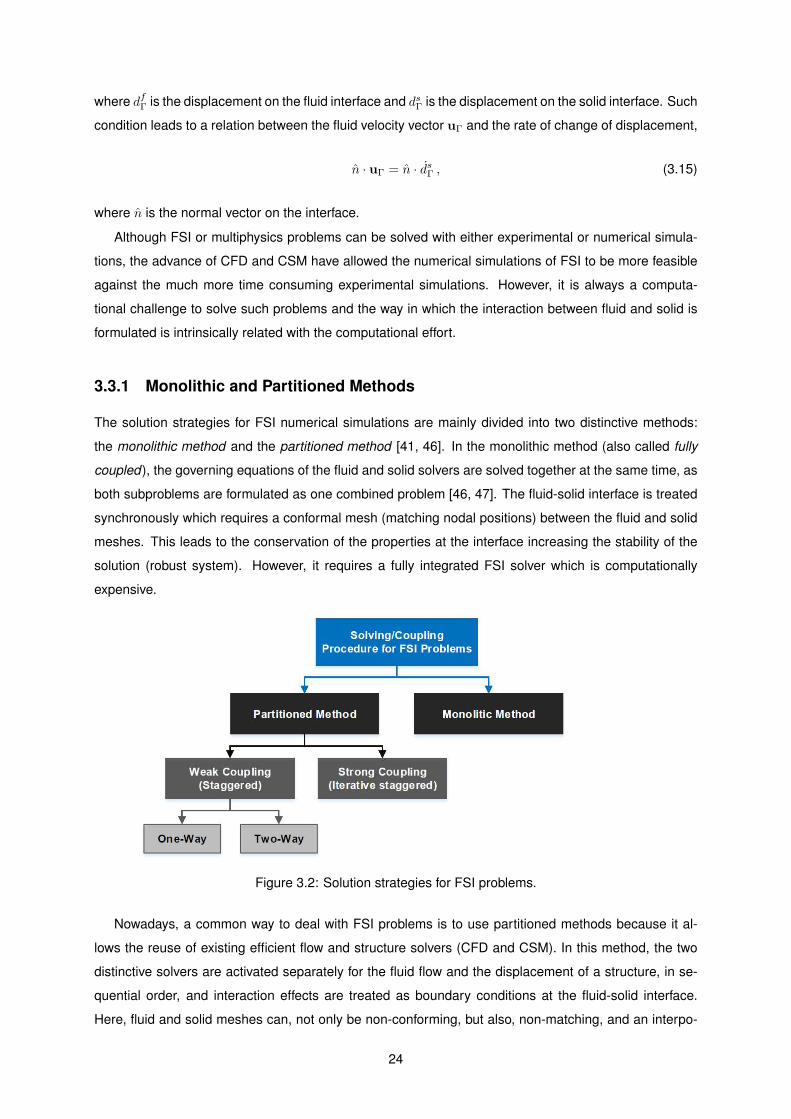
where dfΓ

is the displacement on the fluid interface and dsΓ is the displacement on the solid interface. Such

condition leads to a relation between the fluid velocity vector uΓ and the rate of change of displacement,

n · uΓ = n · dsΓ , (3.15)

where n is the normal vector on the interface.

Although FSI or multiphysics problems can be solved with either experimental or numerical simula-

tions, the advance of CFD and CSM have allowed the numerical simulations of FSI to be more feasible

against the much more time consuming experimental simulations. However, it is always a computa-

tional challenge to solve such problems and the way in which the interaction between fluid and solid is

formulated is intrinsically related with the computational effort.

3.3.1 Monolithic and Partitioned Methods

The solution strategies for FSI numerical simulations are mainly divided into two distinctive methods:

the monolithic method and the partitioned method [41, 46]. In the monolithic method (also called fully

coupled), the governing equations of the fluid and solid solvers are solved together at the same time, as

both subproblems are formulated as one combined problem [46, 47]. The fluid-solid interface is treated

synchronously which requires a conformal mesh (matching nodal positions) between the fluid and solid

meshes. This leads to the conservation of the properties at the interface increasing the stability of the

solution (robust system). However, it requires a fully integrated FSI solver which is computationally

expensive.

Figure 3.2: Solution strategies for FSI problems.

Nowadays, a common way to deal with FSI problems is to use partitioned methods because it al-

lows the reuse of existing efficient flow and structure solvers (CFD and CSM). In this method, the two

distinctive solvers are activated separately for the fluid flow and the displacement of a structure, in se-

quential order, and interaction effects are treated as boundary conditions at the fluid-solid interface.

Here, fluid and solid meshes can, not only be non-conforming, but also, non-matching, and an interpo-

24

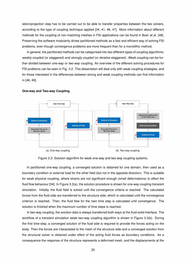
lation/projection step has to be carried out to be able to transfer properties between the two solvers,

according to the type of coupling technique applied [34, 41, 46, 47]. More information about different

methods for the coupling of non-matching meshes in FSI applications can be found in Boer et al. [48].

Preserving the software modularity drives partitioned methods as a fast and efficient way of solving FSI

problems, even though convergence problems are more frequent than for a monolithic method.

In general, the partitioned methods can be categorised into two different types of coupling algorithms:

weakly coupled (or staggered) and strongly coupled (or iterative staggered). Weak coupling can be fur-

ther divided between one-way or two-way coupling. An overview of the different solving procedures for

FSI problems can be seen in Fig. 3.2. This dissertation will deal only with weak coupling strategies, and

for those interested in the differences between strong and weak coupling methods can find information

in [46, 49].

One-way and Two-way Coupling

(a) One-way coupling. (b) Two-way coupling.

Figure 3.3: Solution algorithm for weak one-way and two-way coupling systems.

In partitioned one-way coupling, a converged solution is obtained for one domain, then used as a

boundary condition or external load for the other field (but not in the opposite direction). This is suitable

for weak physical coupling, where strains are not significant enough (small deformations) to affect the

fluid flow behaviour [34]. In Figure 3.3(a), the solution procedure is shown for one-way coupling transient

simulation. Initially, the fluid field is solved until the convergence criteria is reached. The calculated

forces from the fluid side are transferred to the structure side, which is calculated until the convergence

criterion is reached. Then, the fluid flow for the next time step is calculated until convergence. The

solution is finished when the maximum number of time steps is reached.

In two-way coupling, the solution data is always transferred both ways at the fluid-solid interface. The

workflow of a transient simulation weak two-way coupling algorithm is shown in Figure 3.3(b). During

the first time-step, a converged solution of the fluid side is required to provide the forces acting on the

body. Then the forces are interpolated to the mesh of the structure side and a converged solution from

the structural solver is obtained under effect of the acting fluid forces as boundary conditions. As a

consequence the response of the structure represents a deformed mesh, and the displacements at the

25

boundary between structure and fluid are interpolated to the fluid mesh in the next time-step, which

results in the deformation of the fluid domain. This process is repeated until the changes on both fluid

forces and structure displacements fall below a predetermined value. A two-way coupling analysis is

much more accurate for problems with large deflections, where the fluid field is strongly influenced by the

structural deformation. However, comparing with one-way coupling, the simulation needs significantly

more computational time [41].

3.4 Multidisciplinary Design Analysis and Optimisation (MDAO)

The application of MDAO to an aero-structural problem can be made by two approximations, low-fidelity

and high-fidelity. The low-fidelity level of analysis uses simplified numerical models, becoming computa-

tionally efficient (low processing time), and the various disciplines involved may be using reduced levels

of detail, or ignoring certain design factors. Its purpose is to give designers and engineers a general idea

on the performance of the structure in the first stages of the design process. On the other hand, high-

fidelity optimisation occurs when the general design of the structure has been resolved, and designers

and engineers are searching for improvements, such as optimising a rear wing shape for certain ob-

jectives. High-fidelity optimisation uses detailed numerical models and the disciplinary analysis is more

complex and rigorous (e.g. Navier-Stokes and Finite Elements Method). As a result, the computational

resources and time required are much greater, yet it is the high-fidelity analysis that provide an optimal

detailed design.

3.4.1 MDAO Architectures

Overall, the purpose of both low-fidelity and high-fidelity optimisation is to avoid, or bypass the engineers

intuition about the design problem. Based on the results of the individual analysis of the disciplines

(according to the MDAO strategy adopted), the optimisation process might follow a direction in which the

result might be unexpected. Besides achieving an optimal design, the aim of MDAO is to accomplish this

optimisation in the shortest time possible, thus increasing the efficiency of the optimisation procedure.

To this purpose, there are different MDAO architectures (or strategies) that can be more appropriate

according to the design problem. Considerable research has already been performed on the advantages

and disadvantages of particular MDAO strategies, both in the automotive [50, 51, 52, 53] and aerospace

applications [54, 55, 56, 57, 58]. For example, Tedford & Martins [55] and Perez et al. [56] consider

the efficiency of the optimisation algorithm using metrics such as number of iterations, design variable,

coupling variables and accuracy. The purpose of this project is not to fully delve into this, however, issues

concerning Multidisciplinary Design Analysis (MDA) will appear during the course of this dissertation.

3.4.2 Numerical Optimisation Techniques

Optimisation problems are solved using algorithms that consist of an iterative search process. There are

various algorithms that can be used, and the most suitable choice depends on the nature of the problem.

26

If small improvement is desired, and the structure response is likely to be linear, a local optimisation

method based on gradient information may be sufficient. However, for more complex problems where

the response is likely to be non-linear and a global optimum is desired, a method that can find a global

optimum in the face of highly non-linear responses would be required. These methods could range from

indirect method using response surface techniques to a direct optimisation method such as gradient

based local solvers or nature based global methods [50].

Direct Optimisation Methods

Usually, direct optimisation methods are categorised into two general classes: gradient based and non-

gradient based (like for example stochastic schemes or evolutionay based) [51, 58].

The non-gradient based algorithms are zero-order algorithms, which only use objective and con-

straint function values. They are based on a random generation of design points used for local search

procedures and are typically inspired by phenomenons from nature. The most common non-gradient op-

timisation methods are the Genetic Algorithms (GAs), which are probabilistic search techniques based

on the mechanics of natural selection and genetics [3]. GAs have received considerable attention in

recent years as they stand a good chance of finding the global optimum and appear to be well suited for

solving discrete optimisation problems, such as for example, the optimum laminate stacking sequence

of a rear wing [3]. However, they require evaluations of a considerable number of design points, involv-

ing very high computational costs [50, 51, 58]. More information concerning non-gradient optimisation

algorithms can be found in [3, 51, 58]

Gradient based methods can be first-order or second-order algorithms that use first-order and second-

order gradients, respectively. The majority of these methods use an iterative two-step procedure to reach

a local optimum. First, a search direction is obtained by gradient information, and then a line-search is

performed to determine the step size. For convex optimisation problems any local optimum must be

the global one, but for non-convex problems there is no guarantee for this. Yet, an improved estimation

of the global optimum can be achieved if several search procedures, from different starting points are

performed [51]. In general, gradient based algorithms are fast and require relatively small number of

design point evaluations to reach a local optimum (although both function and gradient evaluations are

needed). However, such techniques have shown difficulties solving discrete optimisation problems and

also to be susceptible to numerical noise [51, 58].

Response Surface Optimisation Method (RSM)

The Response Surface Methodology can be described as a method for constructing global approxima-

tions to the system behaviour based on the calculated results from the different design points in the

design space. It has been widely employed as an inexpensive low order approximation of the computa-

tionally expensive (although more accurate) detailed analysis and simulation codes, such as CFD and

FEM. First, initial approximations are obtained by analysing the system response for determined combi-

nations of the design points and then, the approximation model is used inside the optimization loop to

27

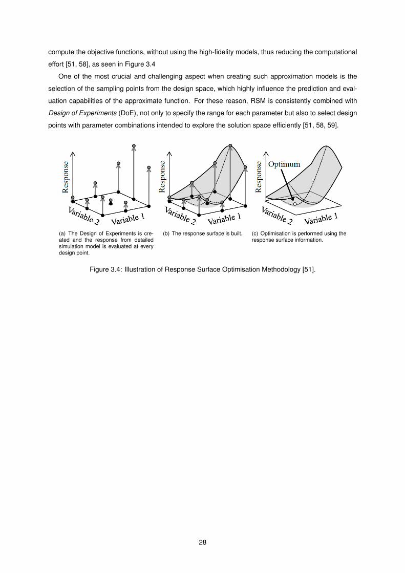
compute the objective functions, without using the high-fidelity models, thus reducing the computational

effort [51, 58], as seen in Figure 3.4

One of the most crucial and challenging aspect when creating such approximation models is the

selection of the sampling points from the design space, which highly influence the prediction and eval-

uation capabilities of the approximate function. For these reason, RSM is consistently combined with

Design of Experiments (DoE), not only to specify the range for each parameter but also to select design

points with parameter combinations intended to explore the solution space efficiently [51, 58, 59].

(a) The Design of Experiments is cre-ated and the response from detailedsimulation model is evaluated at everydesign point.

(b) The response surface is built. (c) Optimisation is performed using theresponse surface information.

Figure 3.4: Illustration of Response Surface Optimisation Methodology [51].

28

Chapter 4

Methodology and Numerical Models

In order to accomplish the objectives proposed for this thesis, appropriate computational tools had to be

chosen, taking into account the computational resources available and the synergy of the different dis-

ciplines involved. In this chapter, description of such tools (numerical models) used to perform the CFD,

CSM, FSI and Optimisation analyses, as well as the CAD geometry generation and parametrisation are

presented, mainly the specific modelling techniques, settings and simplifications adopted regarding both

reliability and quality of the numerical solutions.

4.1 MDAO in ANSYS R© Workbench 14.5

The design of a rear wing is an engineering problem where almost every team in automotive racing (and

high-performance automakers) are challenged by, and the use of Computer-Aided Engineering (CAE)

software has been the primarily choice in order to obtain reliable and efficient products as quick as

possible.

ANSYS R© has been a widely known CAE software of virtual-prototyping and modular simulation sys-

tem, and was used to perform all the analyses presented in this thesis. Its advantages for this work

relied on the fact that ANSYS R© Workbench platform offers specific modules to solve all the disciplines

employed, CAD, CFD, CSM, FSI and Optimisation, without the use of any external software to connect

them. Furthermore, it allowed the user to choose the level of analysis complexity, for each individual

discipline, with extensive settings variety. In the Figure 4.1, an example project schematic of a MDAO

process in ANSYS R© Workbench (Version 14.5) is shown, evidencing its modularity synergy, and cover-

age on the different subjects of interest for the preliminary design of rear wings.

The first module A, Fluent, is the most powerful CFD software tool available in ANSYS R© used to

perform all the CFD analysis in this dissertation. The modules B and D are the ANSYS R© Composite

Prep and Post tools, respectively, designated to the design and analysis of layered composites. These

modules work in combination with module C, Mechanical, which is the structural analysis software with

finite element analysis (FEA) tools. Both Fluent and Mechanical modules can be linked to the module

E, System Coupling, that enables engineers to solve multiphysics problems, and in particular, FSI prob-

29

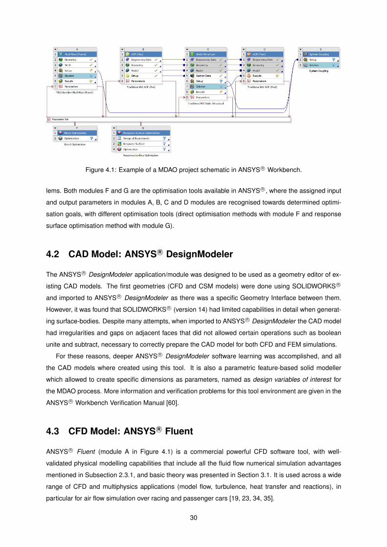
Figure 4.1: Example of a MDAO project schematic in ANSYS R© Workbench.

lems. Both modules F and G are the optimisation tools available in ANSYS R©, where the assigned input

and output parameters in modules A, B, C and D modules are recognised towards determined optimi-

sation goals, with different optimisation tools (direct optimisation methods with module F and response

surface optimisation method with module G).

4.2 CAD Model: ANSYS R© DesignModeler

The ANSYS R© DesignModeler application/module was designed to be used as a geometry editor of ex-

isting CAD models. The first geometries (CFD and CSM models) were done using SOLIDWORKS R©

and imported to ANSYS R© DesignModeler as there was a specific Geometry Interface between them.

However, it was found that SOLIDWORKS R© (version 14) had limited capabilities in detail when generat-

ing surface-bodies. Despite many attempts, when imported to ANSYS R© DesignModeler the CAD model

had irregularities and gaps on adjacent faces that did not allowed certain operations such as boolean

unite and subtract, necessary to correctly prepare the CAD model for both CFD and FEM simulations.

For these reasons, deeper ANSYS R© DesignModeler software learning was accomplished, and all

the CAD models where created using this tool. It is also a parametric feature-based solid modeller

which allowed to create specific dimensions as parameters, named as design variables of interest for

the MDAO process. More information and verification problems for this tool environment are given in the

ANSYS R© Workbench Verification Manual [60].

4.3 CFD Model: ANSYS R© Fluent

ANSYS R© Fluent (module A in Figure 4.1) is a commercial powerful CFD software tool, with well-

validated physical modelling capabilities that include all the fluid flow numerical simulation advantages

mentioned in Subsection 2.3.1, and basic theory was presented in Section 3.1. It is used across a wide

range of CFD and multiphysics applications (model flow, turbulence, heat transfer and reactions), in

particular for air flow simulation over racing and passenger cars [19, 23, 34, 35].

30

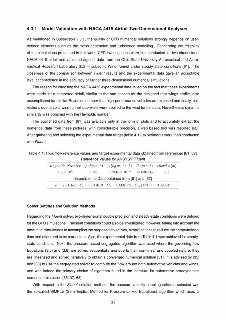
4.3.1 Model Validation with NACA 4415 Airfoil Two-Dimensional Analyses

As mentioned in Subsection 2.3.1, the quality of CFD numerical solutions strongly depends on user-

defined elements such as the mesh generation and turbulence modelling. Concerning the reliability

of the simulations presented in this work, CFD investigations were first conducted for two-dimensional

NACA 4415 airfoil and validated against data from the Ohio State University Aeronautical and Astro-

nautical Research Laboratory 3x5 m subsonic Wind Tunnel under steady state conditions [61]. The

closeness of the comparison between Fluent results and the experimental data gave an acceptable

level of confidence in the accuracy of further three-dimensional numerical simulations.

The reason for choosing the NACA 4415 experimental data relied on the fact that these experiments

were made for a cambered airfoil, similar to the one chosen for the designed rear wings profile, also

accomplished for similar Reynolds number that high-performance vehicles are exposed and finally, cor-

rections due to solid wind tunnel side-walls were applied to the wind tunnel data. Nevertheless dynamic

similarity was obtained with the Reynolds number.

The published data from [61] was available only in the form of plots and to accurately extract the

numerical data from these pictures, with considerable precision, a web based tool was resorted [62].

After gathering and selecting the experimental data target (table 4.1), experiments were then conducted

with Fluent.

Table 4.1: Fluid flow reference values and target experimental data obtained from references [61, 62].

Reference Values for ANSYS R© Fluent

Reynolds Number ρ (kgm−3) µ (kgm−1 s−1) U (ms−1) chord c (m)

1.5× 106 1.225 1.7894× 10−5 73.036735 0.3

Experimental Data obtained from [61] and [62]

α = 2.01 deg Cl = 0.641618 Cd = 0.008178 Cm (1/4 c) = 0.090047

Solver Settings and Solution Methods

Regarding the Fluent solver, two-dimensional double precision and steady-state conditions were defined

for the CFD simulations. Transient conditions could also be investigated, however, taking into account the

amount of simulations to accomplish the proposed objectives, simplifications to reduce the computational

time and effort had to be carried out. Also, the experimental data from Table 4.1 was achieved for steady-

state conditions. Next, the pressure-based segregated algorithm was used where the governing flow

Equations (3.5) and (3.6) are solved sequentially and due to their non-linear and coupled nature, they

are linearised and solved iteratively to obtain a converged numerical solution [31]. It is advised by [35]

and [63] to use the segregated solver to compute the flow around both automotive vehicles and wings,

and was indeed the primary choice of algorithm found in the literature for automotive aerodynamics

numerical simulation [35, 37, 63].

With respect to the Fluent solution methods the pressure-velocity coupling scheme selected was

the so-called SIMPLE (Semi-Implicit Method for Pressure-Linked Equations) algorithm which uses ’a

31

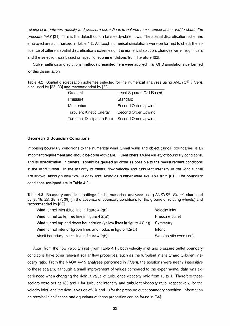
relationship between velocity and pressure corrections to enforce mass conservation and to obtain the

pressure field’ [31]. This is the default option for steady-state flows. The spatial discretisation schemes

employed are summarized in Table 4.2. Although numerical simulations were performed to check the in-

fluence of different spatial discretisations schemes on the numerical solution, changes were insignificant

and the selection was based on specific recommendations from literature [63].

Solver settings and solutions methods presented here were applied in all CFD simulations performed

for this dissertation.

Table 4.2: Spatial discretisation schemes selected for the numerical analyses using ANSYS R© Fluent,

also used by [35, 38] and recommended by [63].

Gradient Least Squares Cell Based

Pressure Standard

Momentum Second Order Upwind

Turbulent Kinetic Energy Second Order Upwind

Turbulent Dissipation Rate Second Order Upwind

Geometry & Boundary Conditions

Imposing boundary conditions to the numerical wind tunnel walls and object (airfoil) boundaries is an

important requirement and should be done with care. Fluent offers a wide variety of boundary conditions,

and its specification, in general, should be geared as close as possible to the measurement conditions

in the wind tunnel. In the majority of cases, flow velocity and turbulent intensity of the wind tunnel

are known, although only flow velocity and Reynolds number were available from [61]. The boundary

conditions assigned are in Table 4.3.

Table 4.3: Boundary conditions settings for the numerical analyses using ANSYS R© Fluent, also used

by [6, 19, 23, 35, 37, 39] (in the absense of boundary conditions for the ground or rotating wheels) and

recommended by [63].

Wind tunnel inlet (blue line in figure 4.2(a)) Velocity inlet

Wind tunnel outlet (red line in figure 4.2(a)) Pressure outlet

Wind tunnel top and down boundaries (yellow lines in figure 4.2(a)) Symmetry

Wind tunnel interior (green lines and nodes in figure 4.2(a)) Interior

Airfoil boundary (black line in figure 4.2(b)) Wall (no-slip condition)

Apart from the flow velocity inlet (from Table 4.1), both velocity inlet and pressure outlet boundary

conditions have other relevant scalar flow properties, such as the turbulent intensity and turbulent vis-

cosity ratio. From the NACA 4415 analyses performed in Fluent, the solutions were nearly insensitive

to these scalars, although a small improvement of values compared to the experimental data was ex-

perienced when changing the default value of turbulence viscosity ratio from 10 to 1. Therefore these

scalars were set as 5% and 1 for turbulent intensity and turbulent viscosity ratio, respectively, for the

velocity inlet, and the default values of 5% and 10 for the pressure outlet boundary condition. Information

on physical significance and equations of these properties can be found in [64].

32

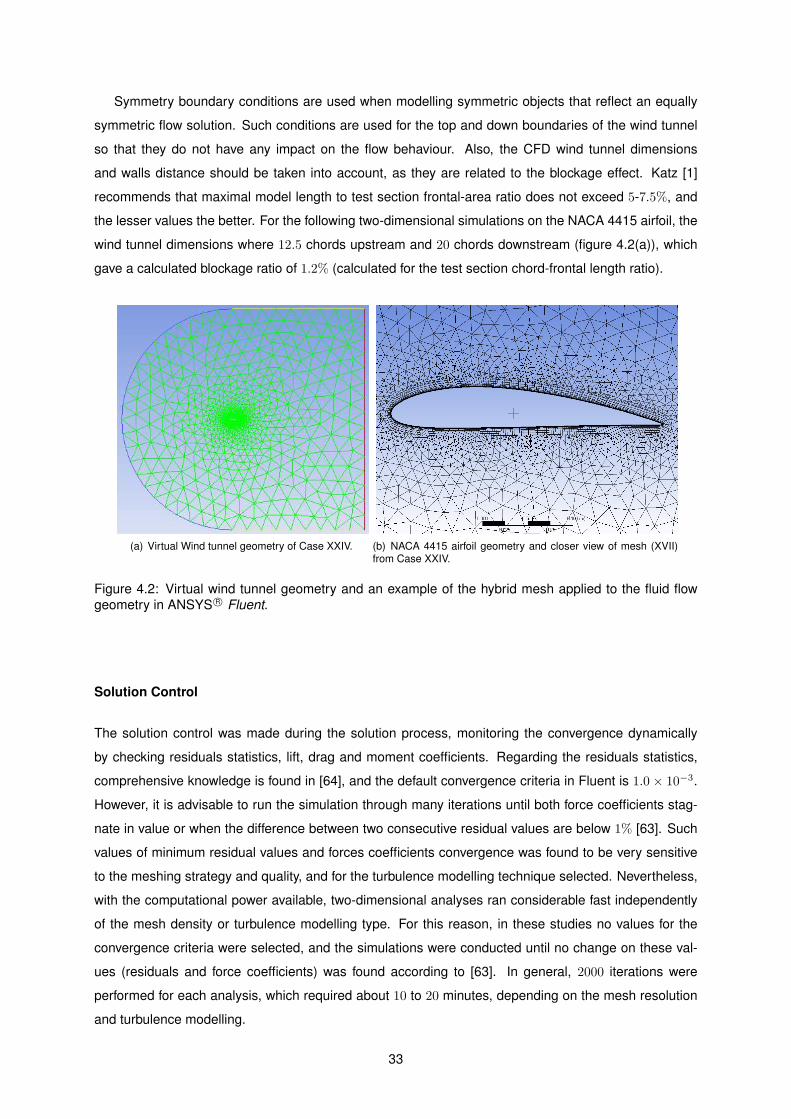
Symmetry boundary conditions are used when modelling symmetric objects that reflect an equally

symmetric flow solution. Such conditions are used for the top and down boundaries of the wind tunnel

so that they do not have any impact on the flow behaviour. Also, the CFD wind tunnel dimensions

and walls distance should be taken into account, as they are related to the blockage effect. Katz [1]

recommends that maximal model length to test section frontal-area ratio does not exceed 5-7.5%, and

the lesser values the better. For the following two-dimensional simulations on the NACA 4415 airfoil, the

wind tunnel dimensions where 12.5 chords upstream and 20 chords downstream (figure 4.2(a)), which

gave a calculated blockage ratio of 1.2% (calculated for the test section chord-frontal length ratio).

(a) Virtual Wind tunnel geometry of Case XXIV. (b) NACA 4415 airfoil geometry and closer view of mesh (XVII)from Case XXIV.

Figure 4.2: Virtual wind tunnel geometry and an example of the hybrid mesh applied to the fluid flow

geometry in ANSYS R© Fluent.

Solution Control

The solution control was made during the solution process, monitoring the convergence dynamically

by checking residuals statistics, lift, drag and moment coefficients. Regarding the residuals statistics,

comprehensive knowledge is found in [64], and the default convergence criteria in Fluent is 1.0 × 10−3.

However, it is advisable to run the simulation through many iterations until both force coefficients stag-

nate in value or when the difference between two consecutive residual values are below 1% [63]. Such

values of minimum residual values and forces coefficients convergence was found to be very sensitive

to the meshing strategy and quality, and for the turbulence modelling technique selected. Nevertheless,

with the computational power available, two-dimensional analyses ran considerable fast independently

of the mesh density or turbulence modelling type. For this reason, in these studies no values for the

convergence criteria were selected, and the simulations were conducted until no change on these val-

ues (residuals and force coefficients) was found according to [63]. In general, 2000 iterations were

performed for each analysis, which required about 10 to 20 minutes, depending on the mesh resolution

and turbulence modelling.

33

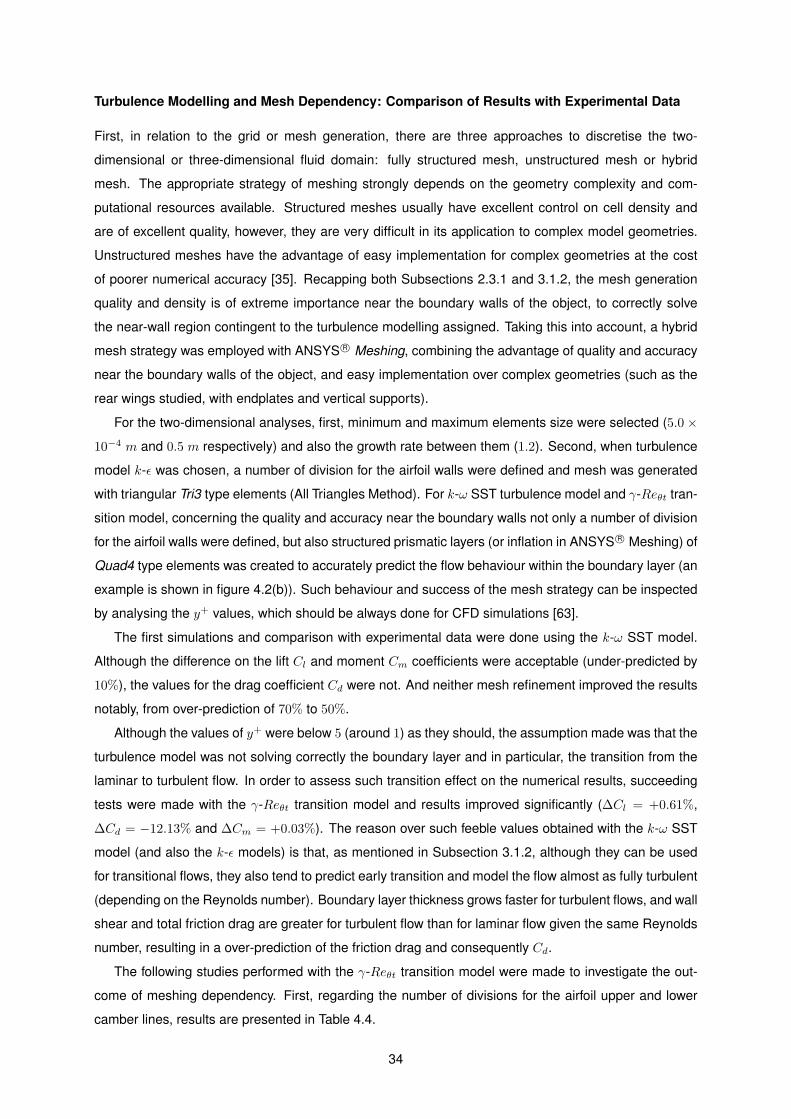
Turbulence Modelling and Mesh Dependency: Comparison of Results with Experimental Data

First, in relation to the grid or mesh generation, there are three approaches to discretise the two-

dimensional or three-dimensional fluid domain: fully structured mesh, unstructured mesh or hybrid

mesh. The appropriate strategy of meshing strongly depends on the geometry complexity and com-

putational resources available. Structured meshes usually have excellent control on cell density and

are of excellent quality, however, they are very difficult in its application to complex model geometries.

Unstructured meshes have the advantage of easy implementation for complex geometries at the cost

of poorer numerical accuracy [35]. Recapping both Subsections 2.3.1 and 3.1.2, the mesh generation

quality and density is of extreme importance near the boundary walls of the object, to correctly solve

the near-wall region contingent to the turbulence modelling assigned. Taking this into account, a hybrid

mesh strategy was employed with ANSYS R© Meshing, combining the advantage of quality and accuracy

near the boundary walls of the object, and easy implementation over complex geometries (such as the

rear wings studied, with endplates and vertical supports).

For the two-dimensional analyses, first, minimum and maximum elements size were selected (5.0×

10−4 m and 0.5 m respectively) and also the growth rate between them (1.2). Second, when turbulence

model k-ǫ was chosen, a number of division for the airfoil walls were defined and mesh was generated

with triangular Tri3 type elements (All Triangles Method). For k-ω SST turbulence model and γ-Reθt tran-

sition model, concerning the quality and accuracy near the boundary walls not only a number of division

for the airfoil walls were defined, but also structured prismatic layers (or inflation in ANSYS R© Meshing) of

Quad4 type elements was created to accurately predict the flow behaviour within the boundary layer (an

example is shown in figure 4.2(b)). Such behaviour and success of the mesh strategy can be inspected

by analysing the y+ values, which should be always done for CFD simulations [63].

The first simulations and comparison with experimental data were done using the k-ω SST model.

Although the difference on the lift Cl and moment Cm coefficients were acceptable (under-predicted by

10%), the values for the drag coefficient Cd were not. And neither mesh refinement improved the results

notably, from over-prediction of 70% to 50%.

Although the values of y+ were below 5 (around 1) as they should, the assumption made was that the

turbulence model was not solving correctly the boundary layer and in particular, the transition from the

laminar to turbulent flow. In order to assess such transition effect on the numerical results, succeeding

tests were made with the γ-Reθt transition model and results improved significantly (∆Cl = +0.61%,

∆Cd = −12.13% and ∆Cm = +0.03%). The reason over such feeble values obtained with the k-ω SST

model (and also the k-ǫ models) is that, as mentioned in Subsection 3.1.2, although they can be used

for transitional flows, they also tend to predict early transition and model the flow almost as fully turbulent

(depending on the Reynolds number). Boundary layer thickness grows faster for turbulent flows, and wall

shear and total friction drag are greater for turbulent flow than for laminar flow given the same Reynolds

number, resulting in a over-prediction of the friction drag and consequently Cd.

The following studies performed with the γ-Reθt transition model were made to investigate the out-

come of meshing dependency. First, regarding the number of divisions for the airfoil upper and lower

camber lines, results are presented in Table 4.4.

34

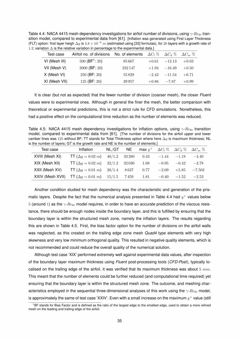
Table 4.4: NACA 4415 mesh dependency investigations for airfoil number of divisions, using γ-Reθt tran-

sition model, compared to experimental data from [61]. [Inflation was generated using First Layer Thickness

(FLT) option: first layer heigh ∆y is 4.8× 10−6 m (estimated using [33] formulas), for 20 layers with a growth rate of

1.2; variation ∆ is the relative variation in percentage to the experimental data.]

Test case Airfoil no. of divisions No. of elements ∆Cl % ∆Cd % ∆Cm %

VI (Mesh III) 500 (BF1: 20) 85 667 +0.61 −12.13 +0.03

VII (Mesh V) 2000 (BF: 20) 232 147 +1.94 −16.49 +0.50

X (Mesh VI) 250 (BF: 20) 55 829 −2.42 −11.54 +6.71

XI (Mesh VII) 125 (BF: 20) 39 957 +0.86 −7.87 +0.99

It is clear (but not as expected) that the fewer number of division (coarser mesh), the closer Fluent

values were to experimental ones. Although in general the finer the mesh, the better comparison with

theoretical or experimental predictions, this is not a strict rule for CFD simulations. Nonetheless, this

had a positive effect on the computational time reduction as the number of elements was reduced.

Table 4.5: NACA 4415 mesh dependency investigations for inflation options, using γ-Reθt transition

model, compared to experimental data from [61]. [The number of divisions for the airfoil upper and lower

camber lines was 125 without BF; TT stands for Total Thickness option where here ∆y is maximum thickness; NL

is the number of layers; GT is the growth rate and NE is the number of elements.]

Test case Inflation NL/GT NE max y+ ∆Cl % ∆Cd % ∆Cm %

XVIII (Mesh XI) TT (∆y = 0.02 m) 40/1.2 33 280 0.43 −1.44 −1.18 −4.40

XIX (Mesh XII) TT (∆y = 0.02 m) 32/1.2 32 030 1.08 −0.95 −0.42 −3.78

XXII (Mesh XV) TT (∆y = 0.01 m) 20/1.4 8 637 0.77 −2.09 +5.85 −7.502

XXIV (Mesh XVII) TT (∆y = 0.01 m) 15/1.5 7 459 1.81 −0.40 −1.52 −2.53

Another condition studied for mesh dependency was the characteristic and generation of the pris-

matic layers. Despite the fact that the numerical analysis presented in Table 4.4 had y+ values below

5 (around 1) as the γ-Reθt model requires, in order to have an accurate prediction of the viscous resis-

tance, there should be enough nodes inside the boundary layer, and this is fulfilled by ensuring that the

boundary layer is within the structured mesh zone, namely the inflation layers. The results regarding

this are shown in Table 4.5. First, the bias factor option for the number of divisions on the airfoil walls

was neglected, as this created on the trailing edge zone mesh Quad4 type elements with very high

skewness and very low minimum orthogonal quality. This resulted in negative quality elements, which is

not recommended and could reduce the overall quality of the numerical solution.

Although test case ’XIX’ performed extremely well against experimental data values, after inspection

of the boundary layer maximum thickness using Fluent post-processing tools (CFD-Post), typically lo-

calised on the trailing edge of the airfoil, it was verified that its maximum thickness was about 5 mm.

This meant that the number of elements could be further reduced (and computational time required) yet

ensuring that the boundary layer is within the structured mesh zone. The outcome, and meshing char-

acteristics employed in the sequential three-dimensional analyses of this work using the γ-Reθt model,

is approximately the same of test case ’XXIV’. Even with a small increase on the maximum y+ value (still

1BF stands for Bias Factor and is defined as the ratio of the largest edge to the smallest edge, used to obtain a more refinedmesh on the leading and trailing edge of the airfoil.

35

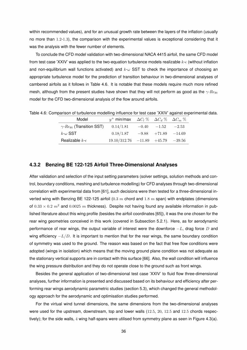
within recommended values), and for an unusual growth rate between the layers of the inflation (usually

no more than 1.2-1.3), the comparison with the experimental values is exceptional considering that it

was the analysis with the fewer number of elements.

To conclude the CFD model validation with two-dimensional NACA 4415 airfoil, the same CFD model

from test case ’XXIV’ was applied to the two-equation turbulence models realizable k-ǫ (without inflation

and non-equilibrium wall functions activated) and k-ω SST to check the importance of choosing an

appropriate turbulence model for the prediction of transition behaviour in two-dimensional analyses of

cambered airfoils as it follows in Table 4.6. It is notable that these models require much more refined

mesh, although from the present studies have shown that they will not perform as good as the γ-Reθt

model for the CFD two-dimensional analysis of the flow around airfoils.

Table 4.6: Comparison of turbulence modelling influence for test case ’XXIV’ against experimental data.

Model y+ min/max ∆Cl % ∆Cd % ∆Cm %

γ-Reθt (Transition SST) 0.14/1.81 −0.40 −1.52 −2.53

k-ω SST 0.18/1.87 −9.88 +71.89 −14.69

Realizable k-ǫ 19.10/312.76 −11.89 +45.79 −39.56

4.3.2 Benzing BE 122-125 Airfoil Three-Dimensional Analyses

After validation and selection of the input setting parameters (solver settings, solution methods and con-

trol, boundary conditions, meshing and turbulence modelling) for CFD analyses through two-dimensional

correlation with experimental data from [61], such decisions were then tested for a three-dimensional in-

verted wing with Benzing BE 122-125 airfoil (0.3 m chord and 1.8 m span) with endplates (dimensions

of 0.33 × 0.2 m2 and 0.0025 m thickness). Despite not having found any available information in pub-

lished literature about this wing profile (besides the airfoil coordinates [65]), it was the one chosen for the

rear wing geometries conceived in this work (covered in Subsection 5.2.1). Here, as for aerodynamic

performance of rear wings, the output variable of interest were the downforce −L, drag force D and

wing efficiency −L/D. It is important to mention that for the rear wings, the same boundary condition

of symmetry was used to the ground. The reason was based on the fact that free flow conditions were

adopted (wings in isolation) which means that the moving ground plane condition was not adequate as

the stationary vertical supports are in contact with this surface [66]. Also, the wall condition will influence

the wing pressure distribution and they do not operate close to the ground such as front wings.

Besides the general application of two-dimensional test case ’XXIV’ to fluid flow three-dimensional

analyses, further information is presented and discussed based on its behaviour and efficiency after per-

forming rear wings aerodynamic parametric studies (section 5.3), which changed the general methodol-

ogy approach for the aerodynamic and optimisation studies performed.

For the virtual wind tunnel dimensions, the same dimensions from the two-dimensional analyses

were used for the upstream, downstream, top and lower walls (12.5, 20, 12.5 and 12.5 chords respec-

tively); for the side walls, 4 wing half-spans were utilised from symmetry plane as seen in Figure 4.3(a).

36

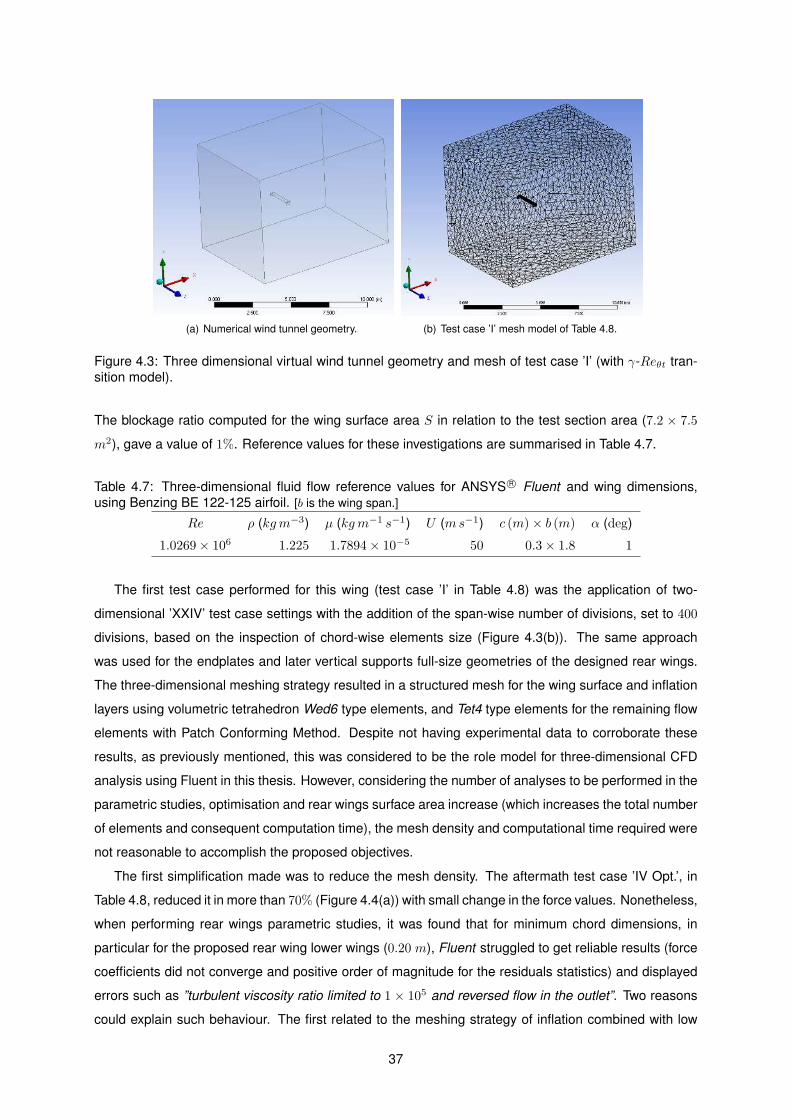
(a) Numerical wind tunnel geometry. (b) Test case ’I’ mesh model of Table 4.8.

Figure 4.3: Three dimensional virtual wind tunnel geometry and mesh of test case ’I’ (with γ-Reθt tran-

sition model).

The blockage ratio computed for the wing surface area S in relation to the test section area (7.2 × 7.5

m2), gave a value of 1%. Reference values for these investigations are summarised in Table 4.7.

Table 4.7: Three-dimensional fluid flow reference values for ANSYS R© Fluent and wing dimensions,

using Benzing BE 122-125 airfoil. [b is the wing span.]

Re ρ (kgm−3) µ (kgm−1 s−1) U (ms−1) c (m)× b (m) α (deg)

1.0269× 106 1.225 1.7894× 10−5 50 0.3× 1.8 1

The first test case performed for this wing (test case ’I’ in Table 4.8) was the application of two-

dimensional ’XXIV’ test case settings with the addition of the span-wise number of divisions, set to 400

divisions, based on the inspection of chord-wise elements size (Figure 4.3(b)). The same approach

was used for the endplates and later vertical supports full-size geometries of the designed rear wings.

The three-dimensional meshing strategy resulted in a structured mesh for the wing surface and inflation

layers using volumetric tetrahedron Wed6 type elements, and Tet4 type elements for the remaining flow

elements with Patch Conforming Method. Despite not having experimental data to corroborate these

results, as previously mentioned, this was considered to be the role model for three-dimensional CFD

analysis using Fluent in this thesis. However, considering the number of analyses to be performed in the

parametric studies, optimisation and rear wings surface area increase (which increases the total number

of elements and consequent computation time), the mesh density and computational time required were

not reasonable to accomplish the proposed objectives.

The first simplification made was to reduce the mesh density. The aftermath test case ’IV Opt.’, in

Table 4.8, reduced it in more than 70% (Figure 4.4(a)) with small change in the force values. Nonetheless,

when performing rear wings parametric studies, it was found that for minimum chord dimensions, in

particular for the proposed rear wing lower wings (0.20 m), Fluent struggled to get reliable results (force

coefficients did not converge and positive order of magnitude for the residuals statistics) and displayed

errors such as ”turbulent viscosity ratio limited to 1 × 105 and reversed flow in the outlet”. Two reasons

could explain such behaviour. The first related to the meshing strategy of inflation combined with low

37

number of divisions (60) and bias factor (10), that resulted in poor quality mesh with extremely high

skewness and very low minimum orthogonal quality elements for the first layers of the inflation and in

particular at the trailing edge of the wing. The second one, associated with the specific γ-Reθt transition

model application for low Reynolds numbers (as a result of reducing the chord dimension). Such model

delays the flow transition and is also extremely dependent on the inlet conditions for low Reynolds

numbers. This can result in a non-converged solution relative to the predominant laminar regime and

consequent problematic transition prediction.

(a) Test case ’IV Opt.’ with 60 (BF:10) number of division forthe airfoil and 200 spanwise. Inflation options are the same oftwo-dimensional test case ’XXIV’.

(b) Test case ’VI Opt.’ with 80 number of division for the airfoiland 200 spanwise. Inflation suppressed.

Figure 4.4: Closer look at the airfoil mesh for optimisation test cases ’IV Opt.’ using γ-Reθt model and

’VI Opt.’ using realizable k-ǫ model with non-equilibrium wall functions in ANSYS R© Meshing.

In order to overcome this and improve significantly poor quality elements from test case ’IV Opt.’

mesh, the decision was to use a turbulence model that doesn’t necessarily need prismatic layers to

guarantee the correct fluid flow computation at the near-wall region through the use of wall functions

(subsection 3.1). The two-equation turbulence model realizable k-ǫ satisfies such requirements. This

turbulence model used in combination with non-equilibrium wall functions is widely used in academic

and industrial applications, and in particular for the automotive road and racing industry [19, 34, 35, 63]

which showed that it is ’possible to achieve good results in terms of integral values (e.g., CD, which are

within 2 − 5%’ [63]. Non-equilibrium wall functions are sensitised to the effects of pressure gradients

and distortion of the velocity profiles [31, 63] and is strongly recommended to be selected for external

aerodynamic simulations by [63].

The third test case presented in Table 4.8 (test case ’II’) is the application of mesh from the first

one (test case I with suppressed inflation) for realizable k-ǫ model in combination with non-equilibrium

wall functions. The resulting mesh, with only Tet4 type elements was significantly reduced in density

as well as computational time required. It performed well against test case ’I’ values using γ-Reθt

transition model with inflation method (within the expected from [63]). The values of y+ where of 10.44 <

y+ < 385.48, although 99% of the wing surface where within 30.00 < y+ < 385.48. Comparing with

two-dimensional numerical analyses, the reason why the realizable k-ǫ model performed a lot better

when compared to the γ-Reθt transition model is related to the type of drag predominance. For two-

dimensional flow around an airfoil, the predominant drag was the friction drag as for three-dimensional

flow around a wing, it was the resulting induced drag from the pressure distribution and vortices at the

wing tip (and endplates).

Despite considerable reduction on the computational time, resources and mesh density, with respect

38

to the rear wings parametric studies and optimisation, it was advised by the supervisor to run these

analyses with a coarser mesh and maximum number of elements about two million. To fulfil such rec-

ommendations, further studies were done and the resulting test case ’VI Opt.’ performed good when

compared to test case ’I’. The y+ values for this test case where of 39.49 < y+ < 479.18 and cross

section view of mesh (and characteristics) can be seen in figure 4.4(b).

Table 4.8: Three-dimensional fluid flow studies with Fluent for different turbulence modelling and mesh-

ing strategies. [NE is the total number of elements; ∆t is the duration of the analysis, for 1000, 1000, 500 and 500

iterations respectively; ∆ is the relative percentage variation calculated in relation to the first ’I (γ-Reθt)’ test case.]

Test case (Model) NE ∆t −L (N) ∆ % D (N) ∆ % −L/D ∆ %

I (γ-Reθt) 6 699 559 8h 938.75 — 59.09 — 15.89 —

IV Opt. (γ-Reθt) 1 805 605 3h 913.45 −2.70 58.23 −1.47 15.69 −1.25

II (realizable k-ǫ) 2 887 477 45min 929.06 −1.03 61.92 +4.77 15.00 −5.55

VI Opt. (realizable k-ǫ) 1 445 577 20min 953.89 +1.61 64.38 +8.95 14.82 −6.74

Based on the discussion and results obtained from these studies, succeeding rear wings aerody-

namic parametric studies (Section 5.3) are presented for both model application of test cases ’IV Opt.’

with γ-Reθt transition model and ’VI Opt.’ with realizable k-ǫ turbulence model combined with non-

equilibrium wall functions. Optimisation analyses were performed only with application of test case ’VI

Opt.’ considering the minimisation of the computational effort. Final results of rear wings aerodynamic

performance were conducted using the test case ’II’ application (with realizable k-ǫ turbulence model)

taking into attention the evidence of small values change when compared to the γ-Reθt transition model

test case ’I’ and the significant computational time advantages.

4.4 CSM Model: ANSYS R© Composite PrepPost and Mechanical

The ANSYS R© Composite PrepPost (ACP) is an add-on module to the existing structural solver (ANSYS R©

Mechanical) dedicated to the modelling of layered composite structures (modules ’B’, ’C’ and ’D’ in fig-

ure 4.1). It has efficient built-in pre- and post-processor tools to accurately represent structure in its

environment (geometry, mesh and boundary conditions), and specifically the representation of the com-

posites (material behaviour, ply definitions, orientations of fibres among others). Another advantage is

the ability that ANSYS R© Composite PrepPost provides in defining composite layup properties as param-

eters (number, orientation and material of laminas) as well as output of structural variables of interest

necessary to conduct structural optimisation studies (displacements, stresses, strains and composites

failure performance). General theory used in both ANSYS R© Composite PrepPost and Mechanical for

the numerical analysis of thin composite structures was mentioned in Section 3.2.

4.4.1 Finite Element Analysis Setup

In this subsection, the structural discipline methodology approach utilised for next chapter succeeding

rear wings numerical analyses is presented. The most important conditions that need to be considered

39

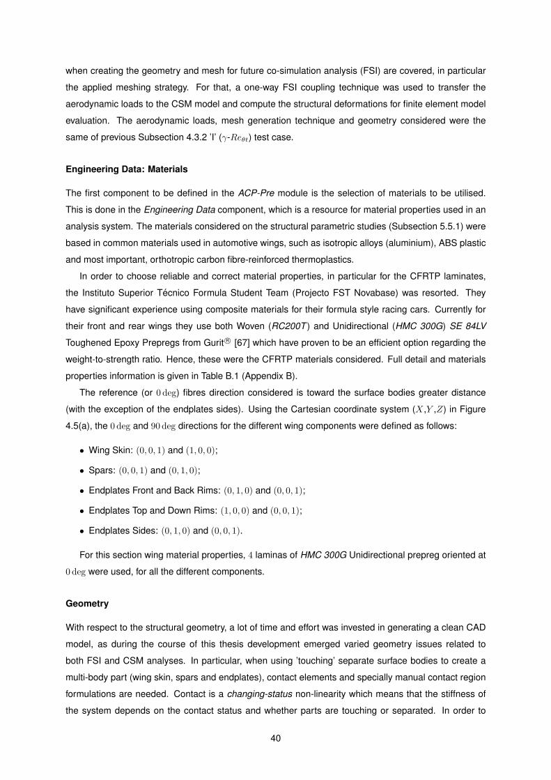
when creating the geometry and mesh for future co-simulation analysis (FSI) are covered, in particular

the applied meshing strategy. For that, a one-way FSI coupling technique was used to transfer the

aerodynamic loads to the CSM model and compute the structural deformations for finite element model

evaluation. The aerodynamic loads, mesh generation technique and geometry considered were the

same of previous Subsection 4.3.2 ’I’ (γ-Reθt) test case.

Engineering Data: Materials

The first component to be defined in the ACP-Pre module is the selection of materials to be utilised.

This is done in the Engineering Data component, which is a resource for material properties used in an

analysis system. The materials considered on the structural parametric studies (Subsection 5.5.1) were

based in common materials used in automotive wings, such as isotropic alloys (aluminium), ABS plastic

and most important, orthotropic carbon fibre-reinforced thermoplastics.

In order to choose reliable and correct material properties, in particular for the CFRTP laminates,

the Instituto Superior Tecnico Formula Student Team (Projecto FST Novabase) was resorted. They

have significant experience using composite materials for their formula style racing cars. Currently for

their front and rear wings they use both Woven (RC200T ) and Unidirectional (HMC 300G) SE 84LV

Toughened Epoxy Prepregs from Gurit R© [67] which have proven to be an efficient option regarding the

weight-to-strength ratio. Hence, these were the CFRTP materials considered. Full detail and materials

properties information is given in Table B.1 (Appendix B).

The reference (or 0 deg) fibres direction considered is toward the surface bodies greater distance

(with the exception of the endplates sides). Using the Cartesian coordinate system (X,Y ,Z) in Figure

4.5(a), the 0 deg and 90 deg directions for the different wing components were defined as follows:

• Wing Skin: (0, 0, 1) and (1, 0, 0);

• Spars: (0, 0, 1) and (0, 1, 0);

• Endplates Front and Back Rims: (0, 1, 0) and (0, 0, 1);

• Endplates Top and Down Rims: (1, 0, 0) and (0, 0, 1);

• Endplates Sides: (0, 1, 0) and (0, 0, 1).

For this section wing material properties, 4 laminas of HMC 300G Unidirectional prepreg oriented at

0 deg were used, for all the different components.

Geometry

With respect to the structural geometry, a lot of time and effort was invested in generating a clean CAD

model, as during the course of this thesis development emerged varied geometry issues related to

both FSI and CSM analyses. In particular, when using ’touching’ separate surface bodies to create a

multi-body part (wing skin, spars and endplates), contact elements and specially manual contact region

formulations are needed. Contact is a changing-status non-linearity which means that the stiffness of

the system depends on the contact status and whether parts are touching or separated. In order to

40

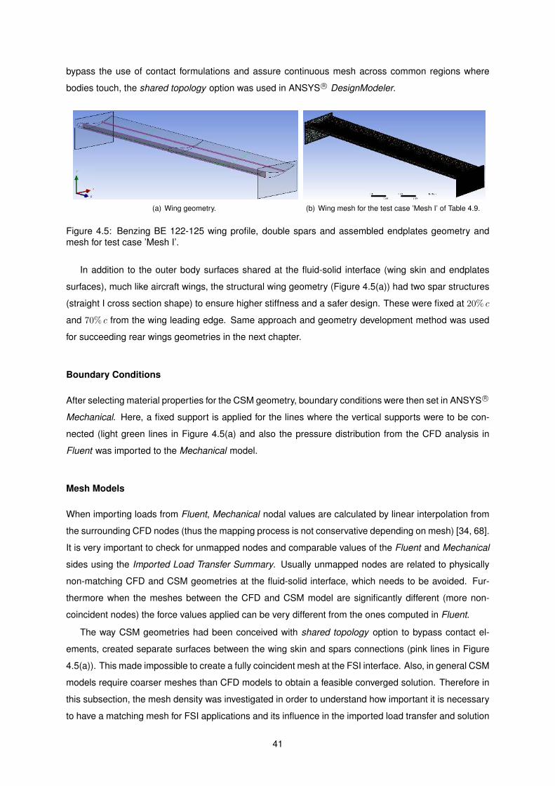
bypass the use of contact formulations and assure continuous mesh across common regions where

bodies touch, the shared topology option was used in ANSYS R© DesignModeler.

(a) Wing geometry. (b) Wing mesh for the test case ’Mesh I’ of Table 4.9.

Figure 4.5: Benzing BE 122-125 wing profile, double spars and assembled endplates geometry and

mesh for test case ’Mesh I’.

In addition to the outer body surfaces shared at the fluid-solid interface (wing skin and endplates

surfaces), much like aircraft wings, the structural wing geometry (Figure 4.5(a)) had two spar structures

(straight I cross section shape) to ensure higher stiffness and a safer design. These were fixed at 20% c

and 70% c from the wing leading edge. Same approach and geometry development method was used

for succeeding rear wings geometries in the next chapter.

Boundary Conditions

After selecting material properties for the CSM geometry, boundary conditions were then set in ANSYS R©

Mechanical. Here, a fixed support is applied for the lines where the vertical supports were to be con-

nected (light green lines in Figure 4.5(a) and also the pressure distribution from the CFD analysis in

Fluent was imported to the Mechanical model.

Mesh Models

When importing loads from Fluent, Mechanical nodal values are calculated by linear interpolation from

the surrounding CFD nodes (thus the mapping process is not conservative depending on mesh) [34, 68].

It is very important to check for unmapped nodes and comparable values of the Fluent and Mechanical

sides using the Imported Load Transfer Summary. Usually unmapped nodes are related to physically

non-matching CFD and CSM geometries at the fluid-solid interface, which needs to be avoided. Fur-

thermore when the meshes between the CFD and CSM model are significantly different (more non-

coincident nodes) the force values applied can be very different from the ones computed in Fluent.

The way CSM geometries had been conceived with shared topology option to bypass contact el-

ements, created separate surfaces between the wing skin and spars connections (pink lines in Figure

4.5(a)). This made impossible to create a fully coincident mesh at the FSI interface. Also, in general CSM

models require coarser meshes than CFD models to obtain a feasible converged solution. Therefore in

this subsection, the mesh density was investigated in order to understand how important it is necessary

to have a matching mesh for FSI applications and its influence in the imported load transfer and solution

41

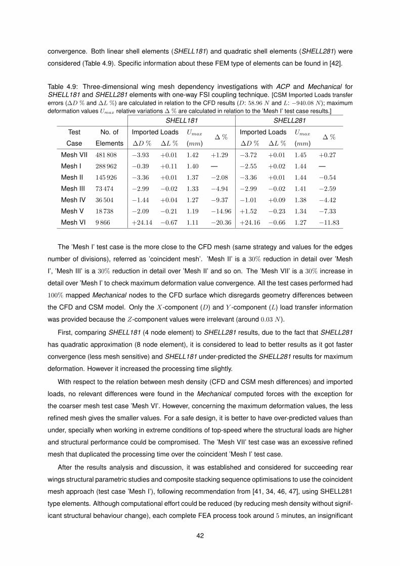
convergence. Both linear shell elements (SHELL181) and quadratic shell elements (SHELL281) were

considered (Table 4.9). Specific information about these FEM type of elements can be found in [42].

Table 4.9: Three-dimensional wing mesh dependency investigations with ACP and Mechanical for

SHELL181 and SHELL281 elements with one-way FSI coupling technique. [CSM Imported Loads transfer

errors (∆D % and ∆L %) are calculated in relation to the CFD results (D: 58.96 N and L: −940.08 N ); maximum

deformation values Umax relative variations ∆ % are calculated in relation to the ’Mesh I’ test case results.]

SHELL181 SHELL281

Test

Case

No. of

Elements

Imported Loads Umax∆ %

Imported Loads Umax∆ %

∆D % ∆L % (mm) ∆D % ∆L % (mm)

Mesh VII 481 808 −3.93 +0.01 1.42 +1.29 −3.72 +0.01 1.45 +0.27

Mesh I 288 962 −0.39 +0.11 1.40 — −2.55 +0.02 1.44 —

Mesh II 145 926 −3.36 +0.01 1.37 −2.08 −3.36 +0.01 1.44 −0.54

Mesh III 73 474 −2.99 −0.02 1.33 −4.94 −2.99 −0.02 1.41 −2.59

Mesh IV 36 504 −1.44 +0.04 1.27 −9.37 −1.01 +0.09 1.38 −4.42

Mesh V 18 738 −2.09 −0.21 1.19 −14.96 +1.52 −0.23 1.34 −7.33

Mesh VI 9 866 +24.14 −0.67 1.11 −20.36 +24.16 −0.66 1.27 −11.83

The ’Mesh I’ test case is the more close to the CFD mesh (same strategy and values for the edges

number of divisions), referred as ’coincident mesh’. ’Mesh II’ is a 30% reduction in detail over ’Mesh

I’, ’Mesh III’ is a 30% reduction in detail over ’Mesh II’ and so on. The ’Mesh VII’ is a 30% increase in

detail over ’Mesh I’ to check maximum deformation value convergence. All the test cases performed had

100% mapped Mechanical nodes to the CFD surface which disregards geometry differences between

the CFD and CSM model. Only the X-component (D) and Y -component (L) load transfer information

was provided because the Z-component values were irrelevant (around 0.03 N ).

First, comparing SHELL181 (4 node element) to SHELL281 results, due to the fact that SHELL281

has quadratic approximation (8 node element), it is considered to lead to better results as it got faster

convergence (less mesh sensitive) and SHELL181 under-predicted the SHELL281 results for maximum

deformation. However it increased the processing time slightly.

With respect to the relation between mesh density (CFD and CSM mesh differences) and imported

loads, no relevant differences were found in the Mechanical computed forces with the exception for

the coarser mesh test case ’Mesh VI’. However, concerning the maximum deformation values, the less

refined mesh gives the smaller values. For a safe design, it is better to have over-predicted values than

under, specially when working in extreme conditions of top-speed where the structural loads are higher

and structural performance could be compromised. The ’Mesh VII’ test case was an excessive refined

mesh that duplicated the processing time over the coincident ’Mesh I’ test case.

After the results analysis and discussion, it was established and considered for succeeding rear

wings structural parametric studies and composite stacking sequence optimisations to use the coincident

mesh approach (test case ’Mesh I’), following recommendation from [41, 34, 46, 47], using SHELL281

type elements. Although computational effort could be reduced (by reducing mesh density without signif-

icant structural behaviour change), each complete FEA process took around 5 minutes, an insignificant

42

value compared to the CFD analyses and it was decided that there was no need to further simplify the

structural model.

4.5 FSI Model: ANSYS R© System Coupling

In ANSYS R© Workbench there are two different approaches to solve FSI problems, a straightforward

technique for one-way coupling (used in the CSM analyses performed in Section 4.4), and for a fully

coupled iterative solution at each time step, using the System Coupling to perform both one-way and

two-way FSI analyses.

Description on the model validity, surface mapping and load transfer accuracy when solving one-way

FSI problems with the straightforward technique was covered in the previous Subsection 4.4.1. In this

section, the process of using the System Coupling to solve both one-way and two-way FSI problems is

explained. Also, a simple non-qualitative problem was conducted in order to understand and evaluate

the computational efficiency in resources when using each one of these techniques (with and without

the System Coupling) to establish the FSI procedure for the following next chapter structural parametric

and optimisation analyses.

Workflow

In order to use the System Coupling module to conduct FSI analyses in ANSYS R© Workbench, ad-

ditional boundary conditions need to be defined in Fluent and Mechanical components. In Fluent, a

System Coupling type dynamic mesh zone for the fluid-solid interface needs to be created, and in Me-

chanical, a Fluid Solid Interface boundary condition is also needed so that the System Coupling can

collect necessary information for the analysis.

By connecting the setup components from Fluent and Mechanical to the System Coupling setup

(Figure 4.1), a participant system is developed by collecting numerical conditions and information from

the coupling participants to identify the fluid-structure interface and synchronize the whole setup of sim-

ulation. The workflow of one-way and two-way coupling techniques were briefly explained in Subsection

3.3.1, and the general procedure of simulation setup in System Coupling consists of three steps:

• Analysis Settings: includes the definition of the coupling initialization (program controlled) and the

duration controls defined by the number of steps and its controls (minimum and maximum coupling

iterations for each time step;

• Data Transfers: incorporation and management of the data transfer sequence between the two nu-

merical solvers (Fluent and Mechanical). This data transfer process is dependent on the coupling

technique adopted. One-way coupling analysis is carried out using a single data transfer from

Fluent (force variable) to Mechanical (also force variable). Besides this data transfer, two-way

coupling has data transfer in both directions, with the addition of a data transfer from Mechanical

(incremental displacement variable) to Fluent (displacement variable). Also Data Transfer Control

can be defined (under relaxation factor and convergence target);

43

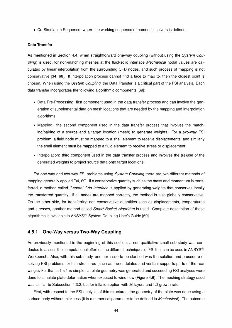
• Co-Simulation Sequence: where the working sequence of numerical solvers is defined.

Data Transfer

As mentioned in Section 4.4, when straightforward one-way coupling (without using the System Cou-

pling) is used, for non-matching meshes at the fluid-solid interface Mechanical nodal values are cal-

culated by linear interpolation from the surrounding CFD nodes, and such process of mapping is not

conservative [34, 68]. If interpolation process cannot find a face to map to, then the closest point is

chosen. When using the System Coupling, the Data Transfer is a critical part of the FSI analysis. Each

data transfer incorporates the following algorithmic components [69]:

• Data Pre-Processing: first component used in the data transfer process and can involve the gen-

eration of supplemental data on mesh locations that are needed by the mapping and interpolation

algorithms;

• Mapping: the second component used in the data transfer process that involves the match-

ing/pairing of a source and a target location (mesh) to generate weights. For a two-way FSI

problem, a fluid node must be mapped to a shell element to receive displacements, and similarly

the shell element must be mapped to a fluid element to receive stress or displacement;

• Interpolation: third component used in the data transfer process and involves the (re)use of the

generated weights to project source data onto target locations.

For one-way and two-way FSI problems using System Coupling there are two different methods of

mapping generally applied [34, 69]. If a conservative quantity such as the mass and momentum is trans-

ferred, a method called General Grid Interface is applied by generating weights that conserves locally

the transferred quantity. If all nodes are mapped correctly, the method is also globally conservative.

On the other side, for transferring non-conservative quantities such as displacements, temperatures

and stresses, another method called Smart Bucket Algorithm is used. Complete description of these

algorithms is available in ANSYS R© System Coupling User’s Guide [69].

4.5.1 One-Way versus Two-Way Coupling

As previously mentioned in the beginning of this section, a non-qualitative small sub-study was con-

ducted to assess the computational effort on the different techniques of FSI that can be used in ANSYS R©

Workbench. Also, with this sub-study, another issue to be clarified was the solution and procedure of

solving FSI problems for thin structures (such as the endplates and vertical supports parts of the rear

wings). For that, a 1× 1 m simple flat plate geometry was generated and succeeding FSI analyses were

done to simulate plate deformation when exposed to wind flow (Figure 4.6). The meshing strategy used

was similar to Subsection 4.3.2, but for inflation option with 30 layers and 1.2 growth rate.

First, with respect to the FSI analysis of thin structures, the geometry of the plate was done using a

surface-body without thickness (it is a numerical parameter to be defined in Mechanical). The outcome

44

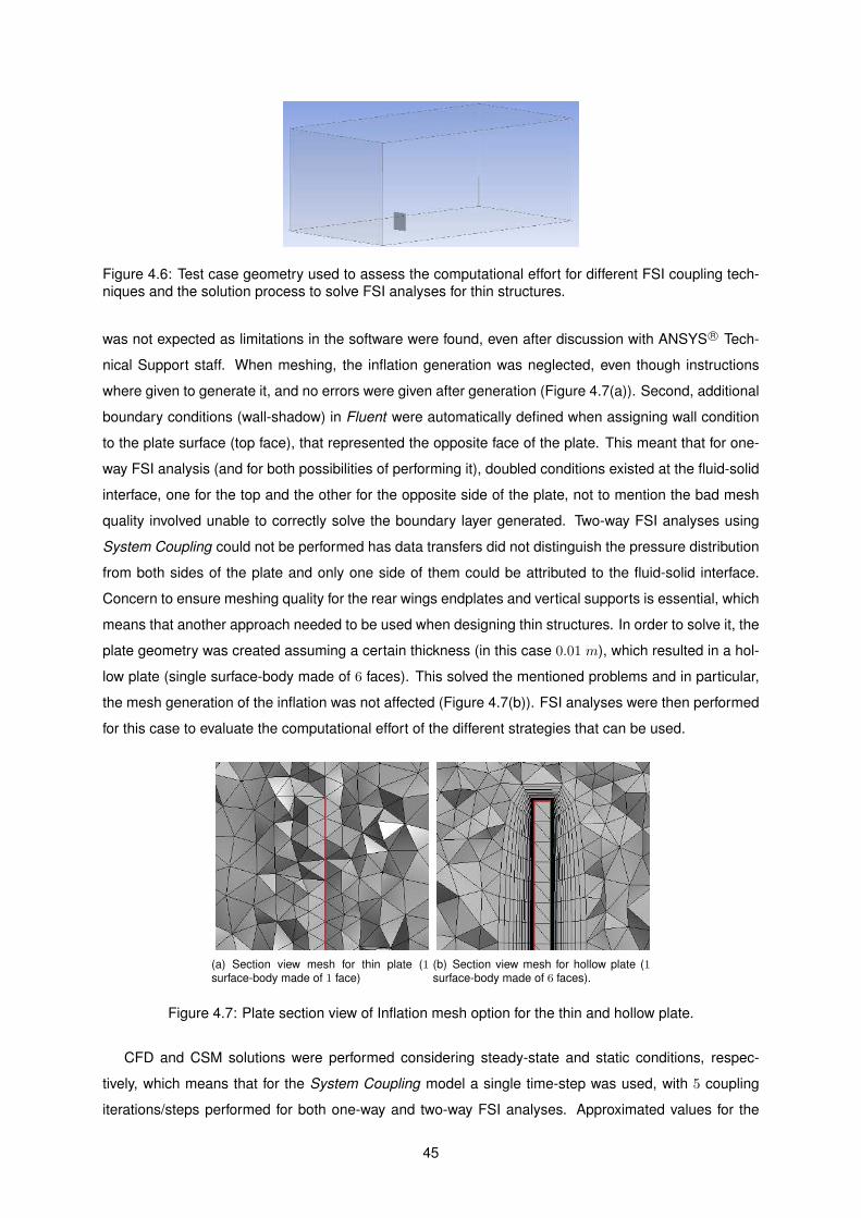
Figure 4.6: Test case geometry used to assess the computational effort for different FSI coupling tech-

niques and the solution process to solve FSI analyses for thin structures.

was not expected as limitations in the software were found, even after discussion with ANSYS R© Tech-

nical Support staff. When meshing, the inflation generation was neglected, even though instructions

where given to generate it, and no errors were given after generation (Figure 4.7(a)). Second, additional

boundary conditions (wall-shadow) in Fluent were automatically defined when assigning wall condition

to the plate surface (top face), that represented the opposite face of the plate. This meant that for one-

way FSI analysis (and for both possibilities of performing it), doubled conditions existed at the fluid-solid

interface, one for the top and the other for the opposite side of the plate, not to mention the bad mesh

quality involved unable to correctly solve the boundary layer generated. Two-way FSI analyses using

System Coupling could not be performed has data transfers did not distinguish the pressure distribution

from both sides of the plate and only one side of them could be attributed to the fluid-solid interface.

Concern to ensure meshing quality for the rear wings endplates and vertical supports is essential, which

means that another approach needed to be used when designing thin structures. In order to solve it, the

plate geometry was created assuming a certain thickness (in this case 0.01 m), which resulted in a hol-

low plate (single surface-body made of 6 faces). This solved the mentioned problems and in particular,

the mesh generation of the inflation was not affected (Figure 4.7(b)). FSI analyses were then performed

for this case to evaluate the computational effort of the different strategies that can be used.

(a) Section view mesh for thin plate (1surface-body made of 1 face)

(b) Section view mesh for hollow plate (1surface-body made of 6 faces).

Figure 4.7: Plate section view of Inflation mesh option for the thin and hollow plate.

CFD and CSM solutions were performed considering steady-state and static conditions, respec-

tively, which means that for the System Coupling model a single time-step was used, with 5 coupling

iterations/steps performed for both one-way and two-way FSI analyses. Approximated values for the

45

computational time required are presented in Table 4.10.

Table 4.10: Approximate values of the computational time when performing FSI analyses using different

available coupling techniques in ANSYS R© Workbench for the plate exposed to wind flow test case.

Fluid-structure interaction technique Computational time

One-way FSI with straightforward technique 8 min

One-way FSI using System Coupling 40 min

Two-way FSI using System Coupling 1 h 30 min

The use of System Coupling to solve FSI problems and specially for two-way analysis proved to

be computationally expensive when compared to the straightforward technique of importing directly the

pressure distribution to the Mechanical component (one-way coupling). Even for one-way coupling,

the System Coupling module proved to be 5 times slower, and for this specific version of ANSYS R©

(14.5) it was advised not to use it for one-way analyses by the ANSYS R© Technical Support staff. The

reason is related to the process that System Coupling uses. For each coupling iteration, the process of

mapping/interpolation is done (which takes more time than the direct approach without using the System

Coupling), than the CFD solution is computed and used to calculate the structural response. For two-

way analyses, also in the same coupling iteration the incremental displacement, or nodal displacements,

are applied to the mesh of the CFD solution and the process of mapping/interpolation occurs again to

compute the CFD solution. This is done for the number of coupling iterations the user defines. It is

not feasible to use more than one coupling iteration when using the System Coupling for one-way FSI

approach, and even so, the solution process is slower than without using the System Coupling. This is

why the ANSYS R© Technical Support staff recommended not to use it for one-way coupling.

Taking into attention the computational resources and in particular the duration of performing FSI

analyses to better fit the objectives proposed for this thesis, the straightforward technique of one-way

coupling was used to perform all the structural parametric and optimisation solutions. Furthermore,

in particular for rear wings, the deformations usually are small, which fits the FSI one-way coupling

approach [34].

4.6 Optimisation Model: ANSYS R© Direct Optimisation

In order to have a complete control and regulation of the optimisation process, where it be regarding the

MDAO strategy to be employed, or the optimiser algorithm, a specific external code would have to be

necessarily used, or produced, and linked to the ANSYS R© Workbench environment. However, due to

time constraints and concern in maintaining the synergy of the disciplinary modules used, the optimi-

sation problems were also conducted inside the ANSYS R© Workbench environment. ANSYS R© Design

Exploration seamlessly integrated different single and multi-objective direct optimisation strategies as

well as response surface generation and optimisation.

Following the investigations and simplifications selected in Subsection 4.5.1, to achieve optimal so-

lutions of both aerodynamic and structural disciplines in a relative short time frame, the MDAO strategy

46

employed followed a sequential optimisation method, where each sub-system (CFD and CSM) had its

own local optimiser. This gave space to employ different optimisation algorithms more suited for each

discipline.

Although response surface optimisation methods have been widely employed and performed consis-

tently well [50], they still are low order approximation models of the high-fidelity codes where the design

space needs to be carefully formulated, as they unconditionally influence the prediction and evaluation

capabilities of the approximate functions. That said, the option was to use the Goal Driven Optimisation

tool with direct optimisation methods that use the high-fidelity CFD and FEM codes, seeking accuracy

and robustness when performing both aerodynamic and structural optimisation of the rear wing designs.

Furthermore, the Direct Optimisation system (module F in Figure 4.1) allowed to monitor and inspect

the optimisation progress towards its feasibility.

The available optimisation methods in the Direct Optimisation system were: Shifted Hammersley

Sampling (Screening), Non-Linear Programming by Quadratic Lagrangian (NLPQL), Mixed-Integer Se-

quential Quadratic Programming (MISQP), Multi-Objective Genetic Algorithm (MOGA), Adaptive Single-

Objective and Adaptive Multi-Objective. Specific information over each method can be seen in [59].

Both aerodynamic and structural disciplines optimisation were performed for a single objective function,

so only single objective optimisation methods were considered. The aerodynamic design variables were

continuous parameters (Section 5.4) as for the structural discipline, these were discrete parameters

(Section 5.6). This was an important condition in choosing appropriate optimisation methods as their

capabilities in handling such deign variables classification varies according to the specific method.

The aerodynamic optimisation method employed was the NLPQL. It provides a more refined ap-

proach than the Screening method and although Adaptative Single-Objective method could also be

used, it was recommended over the NLPQL for simulations with great deal of noise [59]. The NLPQL

is a gradient based single objective optimiser (others output parameters can be defined as constraints)

developed by Klaus Schittkowski, which is based on quasi-Newton methods and suited for local optimi-

sation problems. This method solves constrained non-linear programming problems of the form [59]:

Minimisex

f = f({x}) ,

subject to gk({x}) ≤ 0 , ∀ k = 1, 2, ...,K ,

hl({x}) = 0 , ∀ l = 1, 2, ..., L ,

where {xl} ≤ {x} ≤ {xu} ,

(4.1)

where f({x}) is the objective function, gk({x} and hl({x}) are the system constraints, K and L are the

numbers of inequality and equality constraints, and {xl} and {xu} are the lower and upper bounds of

the continuous design variable x.

With respect to the structural discipline, the available methods that could handle discrete design

variables were the Screening and MISQP. For the same reason explained for the aerodynamic optimi-

sation, the Screening method was considered by [59] being not fully accurate and recommended to be

used only for preliminary designs. Although its accuracy could improve with more sample points, that

47

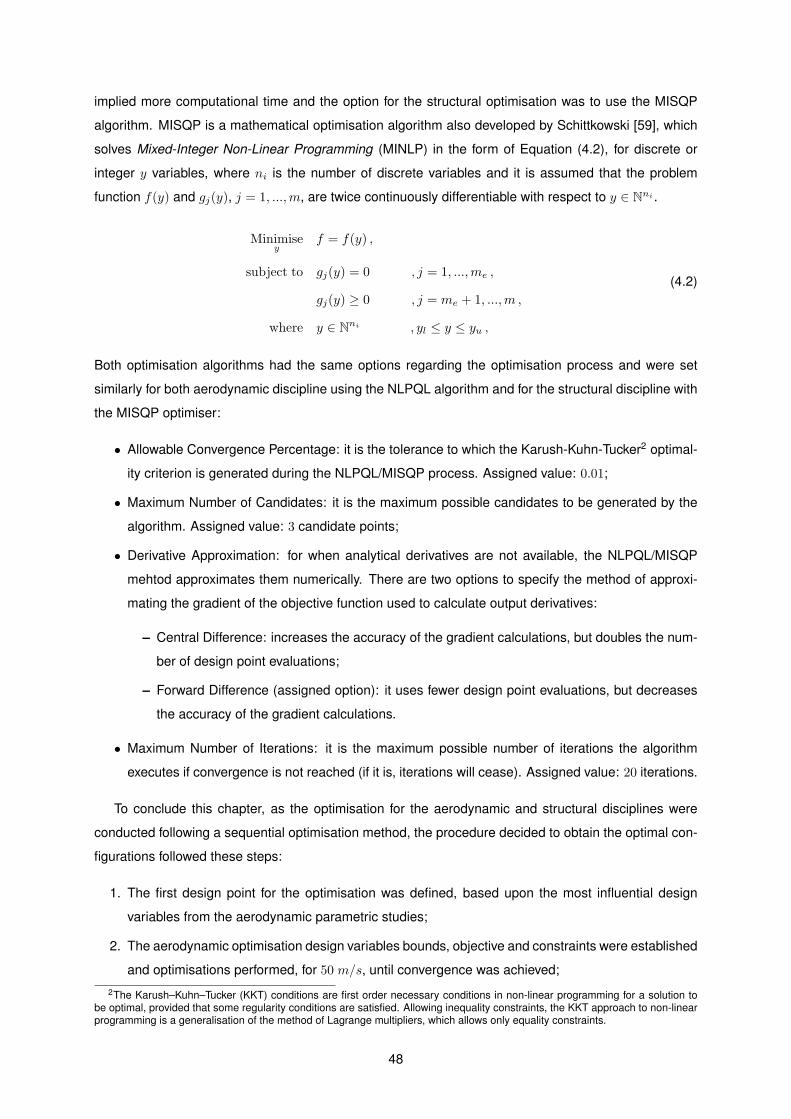
implied more computational time and the option for the structural optimisation was to use the MISQP

algorithm. MISQP is a mathematical optimisation algorithm also developed by Schittkowski [59], which

solves Mixed-Integer Non-Linear Programming (MINLP) in the form of Equation (4.2), for discrete or

integer y variables, where ni is the number of discrete variables and it is assumed that the problem

function f(y) and gj(y), j = 1, ...,m, are twice continuously differentiable with respect to y ∈ Nni .

Minimisey

f = f(y) ,

subject to gj(y) = 0 , j = 1, ...,me ,

gj(y) ≥ 0 , j = me + 1, ...,m ,

where y ∈ Nni , yl ≤ y ≤ yu ,

(4.2)

Both optimisation algorithms had the same options regarding the optimisation process and were set

similarly for both aerodynamic discipline using the NLPQL algorithm and for the structural discipline with

the MISQP optimiser:

• Allowable Convergence Percentage: it is the tolerance to which the Karush-Kuhn-Tucker2 optimal-

ity criterion is generated during the NLPQL/MISQP process. Assigned value: 0.01;

• Maximum Number of Candidates: it is the maximum possible candidates to be generated by the

algorithm. Assigned value: 3 candidate points;

• Derivative Approximation: for when analytical derivatives are not available, the NLPQL/MISQP

mehtod approximates them numerically. There are two options to specify the method of approxi-

mating the gradient of the objective function used to calculate output derivatives:

– Central Difference: increases the accuracy of the gradient calculations, but doubles the num-

ber of design point evaluations;

– Forward Difference (assigned option): it uses fewer design point evaluations, but decreases

the accuracy of the gradient calculations.

• Maximum Number of Iterations: it is the maximum possible number of iterations the algorithm

executes if convergence is not reached (if it is, iterations will cease). Assigned value: 20 iterations.

To conclude this chapter, as the optimisation for the aerodynamic and structural disciplines were

conducted following a sequential optimisation method, the procedure decided to obtain the optimal con-

figurations followed these steps:

1. The first design point for the optimisation was defined, based upon the most influential design

variables from the aerodynamic parametric studies;

2. The aerodynamic optimisation design variables bounds, objective and constraints were established

and optimisations performed, for 50 m/s, until convergence was achieved;

2The Karush–Kuhn–Tucker (KKT) conditions are first order necessary conditions in non-linear programming for a solution tobe optimal, provided that some regularity conditions are satisfied. Allowing inequality constraints, the KKT approach to non-linearprogramming is a generalisation of the method of Lagrange multipliers, which allows only equality constraints.

48

3. Structural parametric studies were run for the best (aerodynamic) candidate design configurations,

but for a velocity considered of 90 m/s (were the aerodynamic loads are more significant);

4. The structural optimisation design variables bounds, objective and constraints were established

and optimisations performed until convergence was achieved.

49

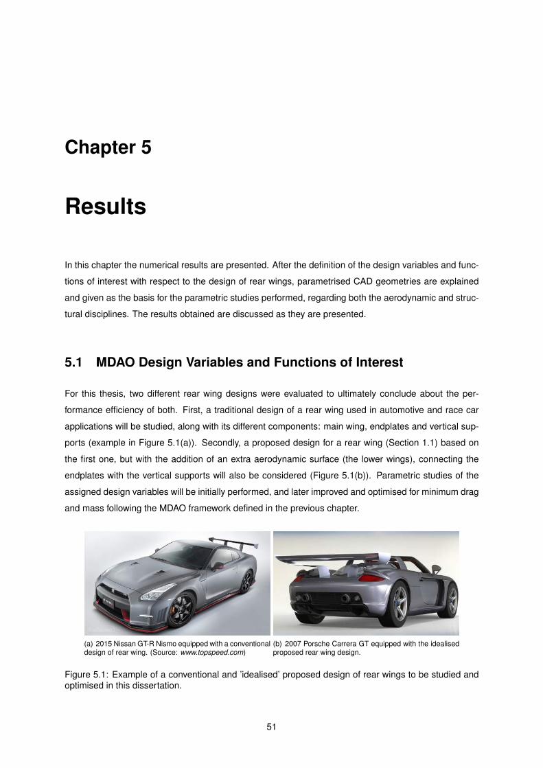
Chapter 5

Results

In this chapter the numerical results are presented. After the definition of the design variables and func-

tions of interest with respect to the design of rear wings, parametrised CAD geometries are explained

and given as the basis for the parametric studies performed, regarding both the aerodynamic and struc-

tural disciplines. The results obtained are discussed as they are presented.

5.1 MDAO Design Variables and Functions of Interest

For this thesis, two different rear wing designs were evaluated to ultimately conclude about the per-

formance efficiency of both. First, a traditional design of a rear wing used in automotive and race car

applications will be studied, along with its different components: main wing, endplates and vertical sup-

ports (example in Figure 5.1(a)). Secondly, a proposed design for a rear wing (Section 1.1) based on

the first one, but with the addition of an extra aerodynamic surface (the lower wings), connecting the

endplates with the vertical supports will also be considered (Figure 5.1(b)). Parametric studies of the

assigned design variables will be initially performed, and later improved and optimised for minimum drag

and mass following the MDAO framework defined in the previous chapter.

(a) 2015 Nissan GT-R Nismo equipped with a conventionaldesign of rear wing. (Source: www.topspeed.com)

(b) 2007 Porsche Carrera GT equipped with the idealisedproposed rear wing design.

Figure 5.1: Example of a conventional and ’idealised’ proposed design of rear wings to be studied and

optimised in this dissertation.

51

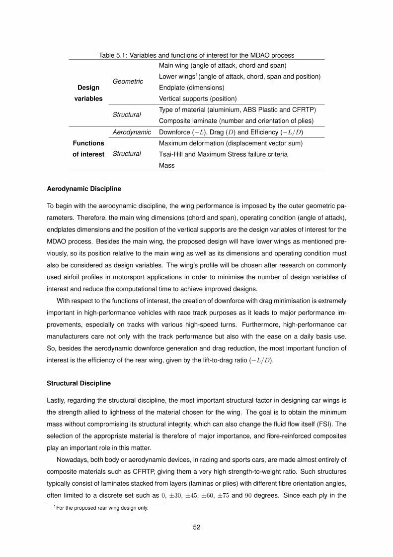
Table 5.1: Variables and functions of interest for the MDAO process

Design

variables

Geometric

Main wing (angle of attack, chord and span)

Lower wings1(angle of attack, chord, span and position)

Endplate (dimensions)

Vertical supports (position)

StructuralType of material (aluminium, ABS Plastic and CFRTP)

Composite laminate (number and orientation of plies)

Functions

of interest

Aerodynamic Downforce (−L), Drag (D) and Efficiency (−L/D)

Structural

Maximum deformation (displacement vector sum)

Tsai-Hill and Maximum Stress failure criteria

Mass

Aerodynamic Discipline

To begin with the aerodynamic discipline, the wing performance is imposed by the outer geometric pa-

rameters. Therefore, the main wing dimensions (chord and span), operating condition (angle of attack),

endplates dimensions and the position of the vertical supports are the design variables of interest for the

MDAO process. Besides the main wing, the proposed design will have lower wings as mentioned pre-

viously, so its position relative to the main wing as well as its dimensions and operating condition must

also be considered as design variables. The wing’s profile will be chosen after research on commonly

used airfoil profiles in motorsport applications in order to minimise the number of design variables of

interest and reduce the computational time to achieve improved designs.

With respect to the functions of interest, the creation of downforce with drag minimisation is extremely

important in high-performance vehicles with race track purposes as it leads to major performance im-

provements, especially on tracks with various high-speed turns. Furthermore, high-performance car

manufacturers care not only with the track performance but also with the ease on a daily basis use.

So, besides the aerodynamic downforce generation and drag reduction, the most important function of

interest is the efficiency of the rear wing, given by the lift-to-drag ratio (−L/D).

Structural Discipline

Lastly, regarding the structural discipline, the most important structural factor in designing car wings is

the strength allied to lightness of the material chosen for the wing. The goal is to obtain the minimum

mass without compromising its structural integrity, which can also change the fluid flow itself (FSI). The

selection of the appropriate material is therefore of major importance, and fibre-reinforced composites

play an important role in this matter.

Nowadays, both body or aerodynamic devices, in racing and sports cars, are made almost entirely of

composite materials such as CFRTP, giving them a very high strength-to-weight ratio. Such structures

typically consist of laminates stacked from layers (laminas or plies) with different fibre orientation angles,

often limited to a discrete set such as 0, ±30, ±45, ±60, ±75 and 90 degrees. Since each ply in the

1For the proposed rear wing design only.

52

composite laminate can have distinct orientations, the optimum composite laminate properties can be

achieved within the MDAO process. Moreover, the number of plies in the composite laminate strongly

influences the mass of the structure and structural response (such as the deformations and stresses).

Concerning the structural integrity of the rear wings, the analysis of failure of the composite layers is

also a function of interest.

The design variables and functions of interest for these case studies are summarised in Table 5.1.

5.2 CAD Parametric Design

After defining the aerodynamic and structural design variables and functions of interest, the baseline

developed parametrised geometries of both traditional and proposed rear wing designs are presented in

Figure 5.2, according to the values summarised in Table 5.2. Furthermore, in the following subsections,

justification and simplifications adopted in the different rear wings components are given and explained.

(a) Traditional rear wing baseline geometry. (b) Proposed rear wing baseline geometry.

Figure 5.2: Baseline parametrised rear wings geometries used for the parametric studies.

Table 5.2: Baseline design variables (parameters) values assigned for the rear wings.

Design variable Value

Wings angle of attack 1 deg

Wings profile chord Main wings: 0.30 m; Lower wings: 0.25 m

Lower wings position Horizontal: 0.0 m; Vertical: −0.2 m

Main wings half-span 0.9 m

Vertical supports position 0.36 m

Endplates length 5% of the main wing chord (from leading and trailing edge)

Endplates upper distance 5% of the main wing chord value

Endplates lower distance 65% of the main wing chord value

5.2.1 Airfoil Selection

The wing profile is a crucial design consideration. Mainly there are two approaches that can be explored:

create it, or choose one from standard airfoils commonly used in motorsport applications. Nevertheless,

much like in motorsport and for high performance road vehicles, the creation of the airfoil is done when

53

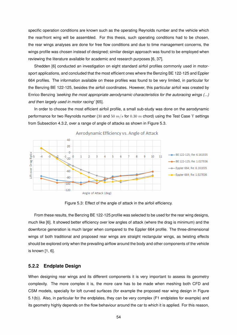
specific operation conditions are known such as the operating Reynolds number and the vehicle which

the rear/front wing will be assembled. For this thesis, such operating conditions had to be chosen,

the rear wings analyses are done for free flow conditions and due to time management concerns, the

wings profile was chosen instead of designed; similar design approach was found to be employed when

reviewing the literature available for academic and research purposes [6, 37].

Shedden [6] conducted an investigation on eight standard airfoil profiles commonly used in motor-

sport applications, and concluded that the most efficient ones where the Benzing BE 122-125 and Eppler

664 profiles. The information available on these profiles was found to be very limited, in particular for

the Benzing BE 122-125, besides the airfoil coordinates. However, this particular airfoil was created by

Enrico Benzing ’seeking the most appropriate aerodynamic characteristics for the autoracing wings (...)

and then largely used in motor racing’ [65].

In order to choose the most efficient airfoil profile, a small sub-study was done on the aerodynamic

performance for two Reynolds number (30 and 50 m/s for 0.30 m chord) using the Test Case ’I’ settings

from Subsection 4.3.2, over a range of angle of attacks as shown in Figure 5.3.

Figure 5.3: Effect of the angle of attack in the airfoil efficiency.

From these results, the Benzing BE 122-125 profile was selected to be used for the rear wing designs,

much like [6]. It showed better efficiency over low angles of attack (where the drag is minimum) and the

downforce generation is much larger when compared to the Eppler 664 profile. The three-dimensional

wings of both traditional and proposed rear wings are straight rectangular wings, as twisting effects

should be explored only when the prevailing airflow around the body and other components of the vehicle

is known [1, 6].

5.2.2 Endplate Design

When designing rear wings and its different components it is very important to assess its geometry

complexity. The more complex it is, the more care has to be made when meshing both CFD and

CSM models, specially for loft curved surfaces (for example the proposed rear wing design in Figure

5.1(b)). Also, in particular for the endplates, they can be very complex (F1 endplates for example) and

its geometry highly depends on the flow behaviour around the car to which it is applied. For this reason,

54

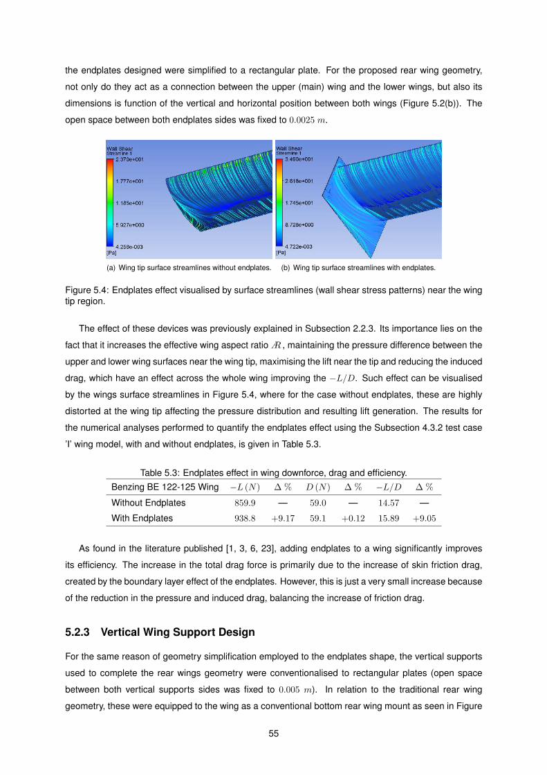
the endplates designed were simplified to a rectangular plate. For the proposed rear wing geometry,

not only do they act as a connection between the upper (main) wing and the lower wings, but also its

dimensions is function of the vertical and horizontal position between both wings (Figure 5.2(b)). The

open space between both endplates sides was fixed to 0.0025 m.

(a) Wing tip surface streamlines without endplates. (b) Wing tip surface streamlines with endplates.

Figure 5.4: Endplates effect visualised by surface streamlines (wall shear stress patterns) near the wing

tip region.

The effect of these devices was previously explained in Subsection 2.2.3. Its importance lies on the

fact that it increases the effective wing aspect ratioA , maintaining the pressure difference between the

upper and lower wing surfaces near the wing tip, maximising the lift near the tip and reducing the induced

drag, which have an effect across the whole wing improving the −L/D. Such effect can be visualised

by the wings surface streamlines in Figure 5.4, where for the case without endplates, these are highly

distorted at the wing tip affecting the pressure distribution and resulting lift generation. The results for

the numerical analyses performed to quantify the endplates effect using the Subsection 4.3.2 test case

’I’ wing model, with and without endplates, is given in Table 5.3.

Table 5.3: Endplates effect in wing downforce, drag and efficiency.

Benzing BE 122-125 Wing −L (N) ∆ % D (N) ∆ % −L/D ∆ %

Without Endplates 859.9 — 59.0 — 14.57 —

With Endplates 938.8 +9.17 59.1 +0.12 15.89 +9.05

As found in the literature published [1, 3, 6, 23], adding endplates to a wing significantly improves

its efficiency. The increase in the total drag force is primarily due to the increase of skin friction drag,

created by the boundary layer effect of the endplates. However, this is just a very small increase because

of the reduction in the pressure and induced drag, balancing the increase of friction drag.

5.2.3 Vertical Wing Support Design

For the same reason of geometry simplification employed to the endplates shape, the vertical supports

used to complete the rear wings geometry were conventionalised to rectangular plates (open space

between both vertical supports sides was fixed to 0.005 m). In relation to the traditional rear wing

geometry, these were equipped to the wing as a conventional bottom rear wing mount as seen in Figure

55

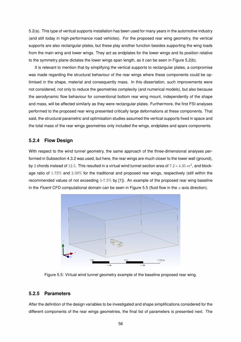
5.2(a). This type of vertical supports installation has been used for many years in the automotive industry

(and still today in high-performance road vehicles). For the proposed rear wing geometry, the vertical

supports are also rectangular plates, but these play another function besides supporting the wing loads

from the main wing and lower wings. They act as endplates for the lower wings and its position relative

to the symmetry plane dictates the lower wings span length, as it can be seen in Figure 5.2(b).

It is relevant to mention that by simplifying the vertical supports to rectangular plates, a compromise

was made regarding the structural behaviour of the rear wings where these components could be op-

timised in the shape, material and consequently mass. In this dissertation, such improvements were

not considered, not only to reduce the geometries complexity (and numerical models), but also because

the aerodynamic flow behaviour for conventional bottom rear wing mount, independently of the shape

and mass, will be affected similarly as they were rectangular plates. Furthermore, the first FSI analyses

performed to the proposed rear wing presented critically large deformations at these components. That

said, the structural parametric and optimisation studies assumed the vertical supports fixed in space and

the total mass of the rear wings geometries only included the wings, endplates and spars components.

5.2.4 Flow Design

With respect to the wind tunnel geometry, the same approach of the three-dimensional analyses per-

formed in Subsection 4.3.2 was used, but here, the rear wings are much closer to the lower wall (ground),

by 2 chords instead of 12.5. This resulted in a virtual wind tunnel section area of 7.2×4.35m2, and block-

age ratio of 1.72% and 2.59% for the traditional and proposed rear wings, respectively (still within the

recommended values of not exceeding 5-7.5% by [1]). An example of the proposed rear wing baseline

in the Fluent CFD computational domain can be seen in Figure 5.5 (fluid flow in the x-axis direction).

Figure 5.5: Virtual wind tunnel geometry example of the baseline proposed rear wing.

5.2.5 Parameters

After the definition of the design variables to be investigated and shape simplifications considered for the

different components of the rear wings geometries, the final list of parameters is presented next. The

56

assigned values for the first design point, called Baseline, are presented in table 5.4.

• Lower wings position: horizontal and vertical position relative to the main wing leading edge line,

of the proposed rear wing only;

• Angle of attack: in relation to the fluid flow x-axis, for the main wings of the traditional and pro-

posed rear wings and also for the lower wings of the proposed design;

• Profile chord: of the main wings of the traditional and proposed rear wings and also for the lower

wings of the proposed design;

• Wing half span: of the main wings of the traditional and proposed rear wings;

• Vertical supports position: in relation to the symmetry plane, for both traditional and proposed

rear wings. Furthermore, for the proposed rear wing this parameter controls the lower wings span

length given by the subtraction of the wing half span and vertical supports position parameters;

• Endplates length: this value is given by the profile chord of the main wing and additional horizontal

distance (in % of the chord value) from the wing leading and trailing edge, for both traditional and

proposed rear wings;

• Endplates upper distance: this value is given by the additional upper vertical distance (in % of

the chord value) from the main wings trailing edge depending of the wing angle of attack, for both

traditional and proposed rear wings;

• Endplates lower distance: for the traditional rear wing, this value is given by the additional lower

vertical distance (in % of the chord value) from the main wing leading edge. For the proposed

design, this value is given by the additional lower vertical distance (also in % of the chord value)

from the lower wings leading edge.

5.3 Aerodynamic Parametric Studies

Results and discussion of the aerodynamic design variables values variation effect for the different rear

wings components are presented in this section. Such effects are given in the form of tables, compared

to the baseline design point of both rear wing designs (relative change).

Table 5.4: Baseline aerodynamic performance values of the traditional and proposed rear wings.

Traditional rear wing Proposed rear wing

−L (N) D (N) −L/D −L (N) D (N) −L/D

γ-Reθt R. k-ǫ γ-Reθt R. k-ǫ γ-Reθt R. k-ǫ γ-Reθt R. k-ǫ γ-Reθt R. k-ǫ γ-Reθt R. k-ǫ

931.7 1028.8 74.2 74.7 12.56 13.78 1289.6 1332.1 110.3 117.9 11.69 11.30

The numerical solutions, as mentioned in Subsection 4.3.2, were calculated with model application

of both test case ’IV Opt.’ with γ-Reθt transition model and ’VI Opt.’ with realizable k-ǫ turbulence model

combined with non-equilibrium wall functions, in order to assess the influence of the turbulence modelling

57

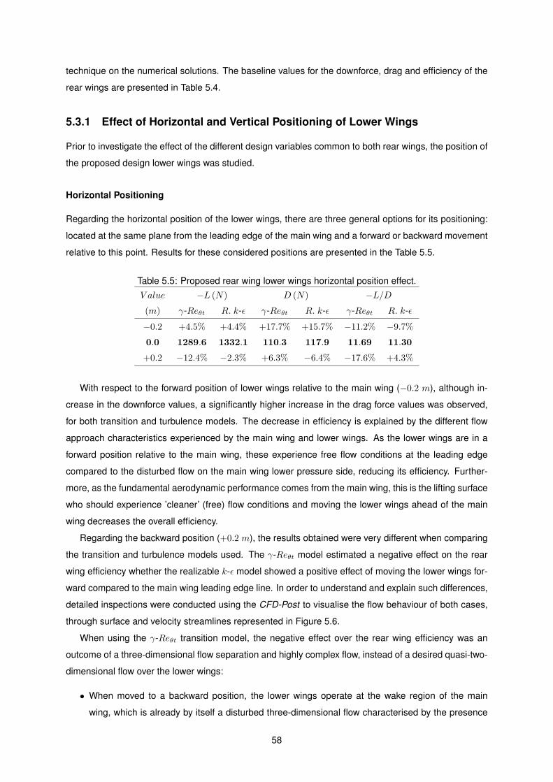
technique on the numerical solutions. The baseline values for the downforce, drag and efficiency of the

rear wings are presented in Table 5.4.

5.3.1 Effect of Horizontal and Vertical Positioning of Lower Wings

Prior to investigate the effect of the different design variables common to both rear wings, the position of

the proposed design lower wings was studied.

Horizontal Positioning

Regarding the horizontal position of the lower wings, there are three general options for its positioning:

located at the same plane from the leading edge of the main wing and a forward or backward movement

relative to this point. Results for these considered positions are presented in the Table 5.5.

Table 5.5: Proposed rear wing lower wings horizontal position effect.

V alue

(m)

−L (N) D (N) −L/D

γ-Reθt R. k-ǫ γ-Reθt R. k-ǫ γ-Reθt R. k-ǫ

−0.2 +4.5% +4.4% +17.7% +15.7% −11.2% −9.7%

0.0 1289.6 1332.1 110.3 117.9 11.69 11.30

+0.2 −12.4% −2.3% +6.3% −6.4% −17.6% +4.3%

With respect to the forward position of lower wings relative to the main wing (−0.2 m), although in-

crease in the downforce values, a significantly higher increase in the drag force values was observed,

for both transition and turbulence models. The decrease in efficiency is explained by the different flow

approach characteristics experienced by the main wing and lower wings. As the lower wings are in a

forward position relative to the main wing, these experience free flow conditions at the leading edge

compared to the disturbed flow on the main wing lower pressure side, reducing its efficiency. Further-

more, as the fundamental aerodynamic performance comes from the main wing, this is the lifting surface

who should experience ’cleaner’ (free) flow conditions and moving the lower wings ahead of the main

wing decreases the overall efficiency.

Regarding the backward position (+0.2 m), the results obtained were very different when comparing

the transition and turbulence models used. The γ-Reθt model estimated a negative effect on the rear

wing efficiency whether the realizable k-ǫ model showed a positive effect of moving the lower wings for-

ward compared to the main wing leading edge line. In order to understand and explain such differences,

detailed inspections were conducted using the CFD-Post to visualise the flow behaviour of both cases,

through surface and velocity streamlines represented in Figure 5.6.

When using the γ-Reθt transition model, the negative effect over the rear wing efficiency was an

outcome of a three-dimensional flow separation and highly complex flow, instead of a desired quasi-two-

dimensional flow over the lower wings:

• When moved to a backward position, the lower wings operate at the wake region of the main

wing, which is already by itself a disturbed three-dimensional flow characterised by the presence

58

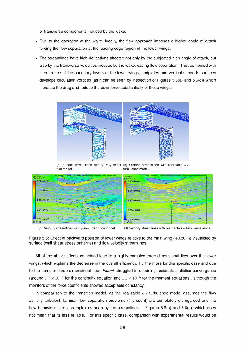
of transverse components induced by the wake;

• Due to the operation at the wake, locally, the flow approach imposes a higher angle of attack

forcing the flow separation at the leading edge region of the lower wings;

• The streamlines have high deflections affected not only by the subjected high angle of attack, but

also by the transverse velocities induced by the wake, easing flow separation. This, combined with

interference of the boundary layers of the lower wings, endplates and vertical supports surfaces

develops circulation vortices (as it can be seen by inspection of Figures 5.6(a) and 5.6(c)) which

increase the drag and reduce the downforce substantially of these wings.

(a) Surface streamlines with γ-Reθt transi-tion model.

(b) Surface streamlines with realizable k-ǫturbulence model.

(c) Velocity streamlines with γ-Reθt transition model. (d) Velocity streamlines with realizable k-ǫ turbulence model.

Figure 5.6: Effect of backward position of lower wings relative to the main wing (+0.20 m) visualised by

surface (wall shear stress patterns) and flow velocity streamlines.

All of the above effects combined lead to a highly complex three-dimensional flow over the lower

wings, which explains the decrease in the overall efficiency. Furthermore for this specific case and due

to the complex three-dimensional flow, Fluent struggled in obtaining residuals statistics convergence

(around 1.7 × 10−3 for the continuity equation and 1.1 × 10−5 for the moment equations), although the

monitors of the force coefficients showed acceptable constancy.

In comparison to the transition model, as the realizable k-ǫ turbulence model assumes the flow

as fully turbulent, laminar flow separation problems (if present) are completely disregarded and the

flow behaviour is less complex as seen by the streamlines in Figures 5.6(b) and 5.6(d), which does

not mean that its less reliable. For this specific case, comparison with experimental results would be

59

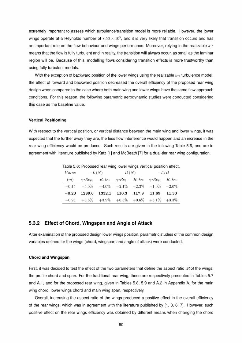
extremely important to assess which turbulence/transition model is more reliable. However, the lower

wings operate at a Reynolds number of 8.56 × 105, and it is very likely that transition occurs and has

an important role on the flow behaviour and wings performance. Moreover, relying in the realizable k-ǫ

means that the flow is fully turbulent and in reality, the transition will always occur, as small as the laminar

region will be. Because of this, modelling flows considering transition effects is more trustworthy than

using fully turbulent models.

With the exception of backward position of the lower wings using the realizable k-ǫ turbulence model,

the effect of forward and backward position decreased the overall efficiency of the proposed rear wing

design when compared to the case where both main wing and lower wings have the same flow approach

conditions. For this reason, the following parametric aerodynamic studies were conducted considering

this case as the baseline value.

Vertical Positioning

With respect to the vertical position, or vertical distance between the main wing and lower wings, it was

expected that the further away they are, the less flow interference would happen and an increase in the

rear wing efficiency would be produced. Such results are given in the following Table 5.6, and are in

agreement with literature published by Katz [1] and McBeath [7] for a dual-tier rear wing configuration.

Table 5.6: Proposed rear wing lower wings vertical position effect.

V alue

(m)

−L (N) D (N) −L/D


−0.15 −4.0% −4.0% −2.1% −2.3% −1.9% −2.0%

−0.20 1289.6 1332.1 110.3 117.9 11.69 11.30

−0.25 +3.6% +3.9% +0.5% +0.6% +3.1% +3.3%

5.3.2 Effect of Chord, Wingspan and Angle of Attack

After examination of the proposed design lower wings position, parametric studies of the common design

variables defined for the wings (chord, wingspan and angle of attack) were conducted.

Chord and Wingspan

First, it was decided to test the effect of the two parameters that define the aspect ratioAof the wings,

the profile chord and span. For the traditional rear wing, these are respectively presented in Tables 5.7

and A.1, and for the proposed rear wing, given in Tables 5.8, 5.9 and A.2 in Appendix A, for the main

wing chord, lower wings chord and main wing span, respectively.

Overall, increasing the aspect ratio of the wings produced a positive effect in the overall efficiency

of the rear wings, which was in agreement with the literature published by [1, 8, 6, 7]. However, such

positive effect on the rear wings efficiency was obtained by different means when changing the chord

60

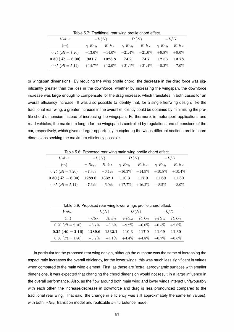
Table 5.7: Traditional rear wing profile chord effect.

V alue

(m)

−L (N) D (N) −L/D


0.25 (A = 7.20) −13.6% −14.0% −21.4% −21.0% +9.8% +9.0%

0.30 (A = 6.00) 931.7 1028.8 74.2 74.7 12.56 13.78

0.35 (A = 5.14) +14.7% +13.0% +21.1% +21.4% −5.2% −7.0%

or wingspan dimensions. By reducing the wing profile chord, the decrease in the drag force was sig-

nificantly greater than the loss in the downforce, whether by increasing the wingspan, the downforce

increase was large enough to compensate for the drag increase, which translates in both cases for an

overall efficiency increase. It was also possible to identify that, for a single tier/wing design, like the

traditional rear wing, a greater increase in the overall efficiency could be obtained by minimising the pro-

file chord dimension instead of increasing the wingspan. Furthermore, in motorsport applications and

road vehicles, the maximum length for the wingspan is controlled by regulations and dimensions of the

car, respectively, which gives a larger opportunity in exploring the wings different sections profile chord

dimensions seeking the maximum efficiency possible.

Table 5.8: Proposed rear wing main wing profile chord effect.

V alue

(m)

−L (N) D (N) −L/D


0.25 (A = 7.20) −7.3% −6.1% −16.3% −14.9% +10.8% +10.4%

0.30 (A = 6.00) 1289.6 1332.1 110.3 117.9 11.69 11.30

0.35 (A = 5.14) +7.6% +6.9% +17.7% +16.2% −8.5% −8.0%

Table 5.9: Proposed rear wing lower wings profile chord effect.

V alue

(m)

−L (N) D (N) −L/D


0.20 (A = 2.70) −8.7% −3.6% −9.2% −6.0% +0.5% +2.6%

0.25 (A = 2.16) 1289.6 1332.1 110.3 117.9 11.69 11.30

0.30 (A = 1.80) +3.7% +4.1% +4.4% +4.8% −0.7% −0.6%

In particular for the proposed rear wing design, although the outcome was the same of increasing the

aspect ratio increases the overall efficiency, for the lower wings, this was much less significant in values

when compared to the main wing element. First, as these are ’extra’ aerodynamic surfaces with smaller

dimensions, it was expected that changing the chord dimension would not result in a large influence in

the overall performance. Also, as the flow around both main wing and lower wings interact unfavourably

with each other, the increase/decrease in downforce and drag is less pronounced compared to the

traditional rear wing. That said, the change in efficiency was still approximately the same (in values),

with both γ-Reθt transition model and realizable k-ǫ turbulence model.

61

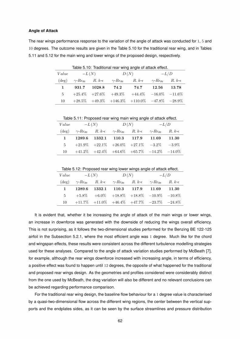
Angle of Attack

The rear wings performance response to the variation of the angle of attack was conducted for 1, 5 and

10 degrees. The outcome results are given in the Table 5.10 for the traditional rear wing, and in Tables

5.11 and 5.12 for the main wing and lower wings of the proposed design, respectively.

Table 5.10: Traditional rear wing angle of attack effect.

V alue

(deg)

−L (N) D (N) −L/D


1 931.7 1028.8 74.2 74.7 12.56 13.78

5 +25.4% +27.6% +49.3% +44.4% −16.0% −11.6%

10 +28.5% +49.3% +146.3% +110.0% −47.8% −28.9%

Table 5.11: Proposed rear wing main wing angle of attack effect.

V alue

(deg)

−L (N) D (N) −L/D


1 1289.6 1332.1 110.3 117.9 11.69 11.30

5 +21.9% +22.1% +26.0% +27.1% −3.2% −3.9%

10 +41.2% +42.4% +64.6% +65.7% −14.2% −14.0%

Table 5.12: Proposed rear wing lower wings angle of attack effect.

V alue

(deg)

−L (N) D (N) −L/D


1 1289.6 1332.1 110.3 117.9 11.69 11.30

5 +5.8% +6.0% +18.8% +18.8% −10.9% −10.8%

10 +11.7% +11.0% +46.4% +47.7% −23.7% −24.8%

It is evident that, whether it be increasing the angle of attack of the main wings or lower wings,

an increase in downforce was generated with the downside of reducing the wings overall efficiency.

This is not surprising, as it follows the two-dimensional studies performed for the Benzing BE 122-125

airfoil in the Subsection 5.2.1, where the most efficient angle was 1 degree. Much like for the chord

and wingspan effects, these results were consistent across the different turbulence modelling strategies

used for these analyses. Compared to the angle of attack variation studies performed by McBeath [7],

for example, although the rear wings downforce increased with increasing angle, in terms of efficiency,

a positive effect was found to happen until 12 degrees, the opposite of what happened for the traditional

and proposed rear wings design. As the geometries and profiles considered were considerably distinct

from the one used by McBeath, the drag variation will also be different and no relevant conclusions can

be achieved regarding performance comparison.

For the traditional rear wing design, the baseline flow behaviour for a 1 degree value is characterised

by a quasi-two-dimensional flow across the different wing regions, the center between the vertical sup-

ports and the endplates sides, as it can be seen by the surface streamlines and pressure distribution

62

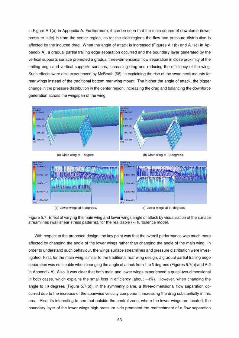
in Figure A.1(a) in Appendix A. Furthermore, it can be seen that the main source of downforce (lower

pressure side) is from the center region, as for the side regions the flow and pressure distribution is

affected by the induced drag. When the angle of attack is increased (Figures A.1(b) and A.1(c) in Ap-

pendix A), a gradual partial trailing edge separation occurred and the boundary layer generated by the

vertical supports surface promoted a gradual three-dimensional flow separation in close proximity of the

trailing edge and vertical supports surfaces, increasing drag and reducing the efficiency of the wing.

Such effects were also experienced by McBeath [66], in explaining the rise of the swan neck mounts for

rear wings instead of the traditional bottom rear wing mount. The higher the angle of attack, the bigger

change in the pressure distribution in the center region, increasing the drag and balancing the downforce

generation across the wingspan of the wing.

(a) Main wing at 1 degree. (b) Main wing at 10 degrees.

(c) Lower wings at 5 degrees. (d) Lower wings at 10 degrees.

Figure 5.7: Effect of varying the main wing and lower wings angle of attack by visualisation of the surface

streamlines (wall shear stress patterns), for the realizable k-ǫ turbulence model.

With respect to the proposed design, the key point was that the overall performance was much more

affected by changing the angle of the lower wings rather than changing the angle of the main wing. In

order to understand such behaviour, the wings surface streamlines and pressure distribution were inves-

tigated. First, for the main wing, similar to the traditional rear wing design, a gradual partial trailing edge

separation was noticeable when changing the angle of attack from 1 to 5 degrees (Figures 5.7(a) and A.2

in Appendix A). Also, it was clear that both main and lower wings experienced a quasi-two-dimensional

in both cases, which explains the small loss in efficiency (about −4%). However, when changing the

angle to 10 degrees (Figure 5.7(b)), in the symmetry plane, a three-dimensional flow separation oc-

curred due to the increase of the spanwise velocity component, increasing the drag substantially in this

area. Also, its interesting to see that outside the central zone, where the lower wings are located, the

boundary layer of the lower wings high-pressure side promoted the reattachment of a flow separation

63

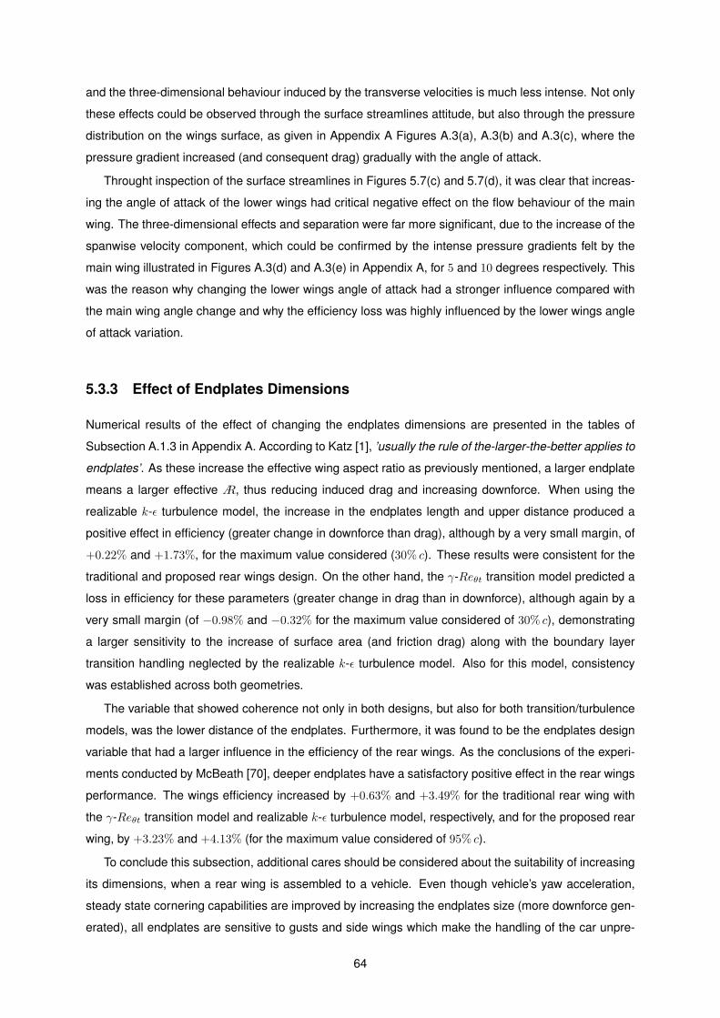
and the three-dimensional behaviour induced by the transverse velocities is much less intense. Not only

these effects could be observed through the surface streamlines attitude, but also through the pressure

distribution on the wings surface, as given in Appendix A Figures A.3(a), A.3(b) and A.3(c), where the

pressure gradient increased (and consequent drag) gradually with the angle of attack.

Throught inspection of the surface streamlines in Figures 5.7(c) and 5.7(d), it was clear that increas-

ing the angle of attack of the lower wings had critical negative effect on the flow behaviour of the main

wing. The three-dimensional effects and separation were far more significant, due to the increase of the

spanwise velocity component, which could be confirmed by the intense pressure gradients felt by the

main wing illustrated in Figures A.3(d) and A.3(e) in Appendix A, for 5 and 10 degrees respectively. This

was the reason why changing the lower wings angle of attack had a stronger influence compared with

the main wing angle change and why the efficiency loss was highly influenced by the lower wings angle

of attack variation.

5.3.3 Effect of Endplates Dimensions

Numerical results of the effect of changing the endplates dimensions are presented in the tables of

Subsection A.1.3 in Appendix A. According to Katz [1], ’usually the rule of the-larger-the-better applies to

endplates’. As these increase the effective wing aspect ratio as previously mentioned, a larger endplate

means a larger effective A, thus reducing induced drag and increasing downforce. When using the

realizable k-ǫ turbulence model, the increase in the endplates length and upper distance produced a

positive effect in efficiency (greater change in downforce than drag), although by a very small margin, of

+0.22% and +1.73%, for the maximum value considered (30% c). These results were consistent for the

traditional and proposed rear wings design. On the other hand, the γ-Reθt transition model predicted a

loss in efficiency for these parameters (greater change in drag than in downforce), although again by a

very small margin (of −0.98% and −0.32% for the maximum value considered of 30% c), demonstrating

a larger sensitivity to the increase of surface area (and friction drag) along with the boundary layer

transition handling neglected by the realizable k-ǫ turbulence model. Also for this model, consistency

was established across both geometries.

The variable that showed coherence not only in both designs, but also for both transition/turbulence

models, was the lower distance of the endplates. Furthermore, it was found to be the endplates design

variable that had a larger influence in the efficiency of the rear wings. As the conclusions of the experi-

ments conducted by McBeath [70], deeper endplates have a satisfactory positive effect in the rear wings

performance. The wings efficiency increased by +0.63% and +3.49% for the traditional rear wing with

the γ-Reθt transition model and realizable k-ǫ turbulence model, respectively, and for the proposed rear

wing, by +3.23% and +4.13% (for the maximum value considered of 95% c).

To conclude this subsection, additional cares should be considered about the suitability of increasing

its dimensions, when a rear wing is assembled to a vehicle. Even though vehicle’s yaw acceleration,

steady state cornering capabilities are improved by increasing the endplates size (more downforce gen-

erated), all endplates are sensitive to gusts and side wings which make the handling of the car unpre-

64

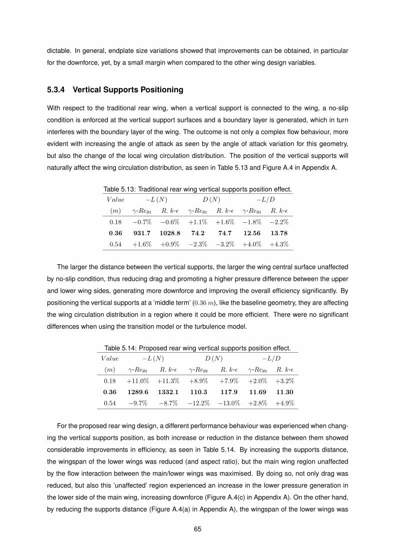
dictable. In general, endplate size variations showed that improvements can be obtained, in particular

for the downforce, yet, by a small margin when compared to the other wing design variables.

5.3.4 Vertical Supports Positioning

With respect to the traditional rear wing, when a vertical support is connected to the wing, a no-slip

condition is enforced at the vertical support surfaces and a boundary layer is generated, which in turn

interferes with the boundary layer of the wing. The outcome is not only a complex flow behaviour, more

evident with increasing the angle of attack as seen by the angle of attack variation for this geometry,

but also the change of the local wing circulation distribution. The position of the vertical supports will

naturally affect the wing circulation distribution, as seen in Table 5.13 and Figure A.4 in Appendix A.

Table 5.13: Traditional rear wing vertical supports position effect.

V alue

(m)

−L (N) D (N) −L/D


0.18 −0.7% −0.6% +1.1% +1.6% −1.8% −2.2%

0.36 931.7 1028.8 74.2 74.7 12.56 13.78

0.54 +1.6% +0.9% −2.3% −3.2% +4.0% +4.3%

The larger the distance between the vertical supports, the larger the wing central surface unaffected

by no-slip condition, thus reducing drag and promoting a higher pressure difference between the upper

and lower wing sides, generating more downforce and improving the overall efficiency significantly. By

positioning the vertical supports at a ’middle term’ (0.36m), like the baseline geometry, they are affecting

the wing circulation distribution in a region where it could be more efficient. There were no significant

differences when using the transition model or the turbulence model.

Table 5.14: Proposed rear wing vertical supports position effect.

V alue

(m)

−L (N) D (N) −L/D


0.18 +11.0% +11.3% +8.9% +7.9% +2.0% +3.2%

0.36 1289.6 1332.1 110.3 117.9 11.69 11.30

0.54 −9.7% −8.7% −12.2% −13.0% +2.8% +4.9%

For the proposed rear wing design, a different performance behaviour was experienced when chang-

ing the vertical supports position, as both increase or reduction in the distance between them showed

considerable improvements in efficiency, as seen in Table 5.14. By increasing the supports distance,

the wingspan of the lower wings was reduced (and aspect ratio), but the main wing region unaffected

by the flow interaction between the main/lower wings was maximised. By doing so, not only drag was

reduced, but also this ’unaffected’ region experienced an increase in the lower pressure generation in

the lower side of the main wing, increasing downforce (Figure A.4(c) in Appendix A). On the other hand,

by reducing the supports distance (Figure A.4(a) in Appendix A), the wingspan of the lower wings was

65

increased (and aspect ratio). The increase in the total lifting surface area meant a significant increase in

downforce when compared to the increase drag. These results were also consistent for both transition

and turbulence models. Finally, by analysing the efficiency values increase, it was noteworthy that a

better efficiency could be achieved, by increasing the vertical supports distance, instead of reducing it,

although by a small margin.

5.4 Aerodynamic Optimisation

Following the parametric studies concluded for the aerodynamic discipline, the next step was the choice

of the optimisation design variables that most positively influenced the aerodynamic performance of

the rear wings. These were the main wings profile chord and angle of attack, wingspan and vertical

supports positioning. In particular for the proposed design, the vertical distance between the main

wing and lower wings also had a strong influence on the overall performance, as the further away they

were, the better the design efficiency. In order to eventually make a correct comparison between both

designs, the objective and constraint functions were defined similarly. Also, the baseline parameters

values were changed in a way that, not only followed the aerodynamic parametric studies seeking better

efficiency, but also to fulfil the optimisation constraint function defined (Downforce > 1200 N ) and reduce

the computational effort in an attempt to approach the optimum design (smaller deviations between the

lower and upper bounds of the optimisation design variables). These design configurations were defined

as the 1st. design point, presented in Table 5.15, where the parameters not mentioned were attributed

as the same of the baseline values and MW, LW and VS are the designations for main wing, lower wings

and vertical supports, respectively.

Table 5.15: Initial design variables values (1st. design point).


Angle of attack = 5.5 deg

Profile chord = 0.27 m

VS position = 0.6 m

−L = 1236.6 N

D = 93.1 N

−L/D = 13.29

MW angle of attack = 2.5 deg −L = 1234.2 N

D = 94.8 N

−L/D = 13.01

MW profile chord = 0.27 m

LW profile chord = 0.23 m

LW vertical position = −0.25 m

VS position = 0.6 m

In Table 5.16 are presented the definition of the optimisation objective and constraint functions and

design variables lower (LB) and upper bounds (UB). Taking into attention the computational effort, due

to time constraints, in the optimisation process of the proposed rear wing design not all of the design

variables from Table 5.15 were considered (only the same of the traditional design). It is also important

to refer that the decisions about the ’best candidates’ (candidate points) was made not only towards

the objective function, that is minimising drag, but also taking into attention the overall performance

(efficiency −L/D) of the rear wings, as advised by Aiguabella [10].

Aerodynamic optimisation results after convergence are presented in Tables 5.17 and 5.18 for the

traditional and proposed rear wing designs, respectively, where AoA, PC and PL are the designations

66

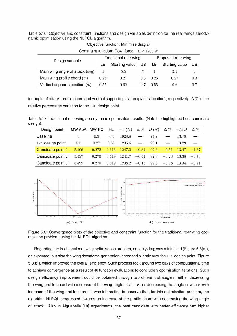
Table 5.16: Objective and constraint functions and design variables definition for the rear wings aerody-

namic optimisation using the NLPQL algorithm.

Objective function: Minimise drag D

Constraint function: Downforce −L ≥ 1200 N

Design variableTraditional rear wing Proposed rear wing

LB Starting value UB LB Starting value UB

Main wing angle of attack (deg) 4 5.5 7 1 2.5 3

Main wing profile chord (m) 0.25 0.27 0.3 0.25 0.27 0.3

Vertical supports position (m) 0.55 0.62 0.7 0.55 0.6 0.7

for angle of attack, profile chord and vertical supports position (pylons location), respectively. ∆ % is the

relative percentage variation to the 1st. design point.

Table 5.17: Traditional rear wing aerodynamic optimisation results. (Note the highlighted best candidate

design).

Design point MW AoA MW PC PL −L (N ) ∆ % D (N ) ∆ % −L/D ∆ %

Baseline 1 0.3 0.36 1028.8 — 74.7 — 13.78 —

1st. design point 5.5 0.27 0.62 1236.6 — 93.1 — 13.29 —

Candidate point 1 5.406 0.272 0.616 1247.0 +0.84 92.6 −0.51 13.47 +1.37

Candidate point 2 5.497 0.270 0.619 1241.7 +0.41 92.8 −0.28 13.38 +0.70

Candidate point 3 5.499 0.270 0.619 1238.2 +0.13 92.8 −0.28 13.34 +0.41

(a) Drag D. (b) Downforce −L.

Figure 5.8: Convergence plots of the objective and constraint function for the traditional rear wing opti-

misation problem, using the NLPQL algorithm.

Regarding the traditional rear wing optimisation problem, not only drag was minimised (Figure 5.8(a)),

as expected, but also the wing downforce generation increased slightly over the 1st. design point (Figure

5.8(b)), which improved the overall efficiency. Such process took around two days of computational time

to achieve convergence as a result of 46 function evaluations to conclude 3 optimisation iterations. Such

design efficiency improvement could be obtained through two different strategies: either decreasing

the wing profile chord with increase of the wing angle of attack, or decreasing the angle of attack with

increase of the wing profile chord. It was interesting to observe that, for this optimisation problem, the

algorithm NLPQL progressed towards an increase of the profile chord with decreasing the wing angle

of attack. Also in Aiguabella [10] experiments, the best candidate with better efficiency had higher

67

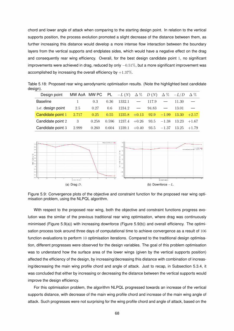
chord and lower angle of attack when comparing to the starting design point. In relation to the vertical

supports position, the process evolution promoted a slight decrease of the distance between them, as

further increasing this distance would develop a more intense flow interaction between the boundary

layers from the vertical supports and endplates sides, which would have a negative effect on the drag

and consequently rear wing efficiency. Overall, for the best design candidate point 1, no significant

improvements were achieved in drag, reduced by only −0.51%, but a more significant improvement was

accomplished by increasing the overall efficiency by +1.37%.

Table 5.18: Proposed rear wing aerodynamic optimisation results. (Note the highlighted best candidate

design).

Design point MW AoA MW PC PL −L (N ) ∆ % D (N ) ∆ % −L/D ∆ %

Baseline 1 0.3 0.36 1332.1 — 117.9 — 11.30 —

1st. design point 2.5 0.27 0.6 1234.2 — 94.83 — 13.01 —

Candidate point 1 2.717 0.25 0.55 1235.8 +0.13 92.9 −1.99 13.30 +2.17

Candidate point 2 3 0.258 0.596 1237.4 +0.26 93.5 −1.38 13.23 +1.67

Candidate point 3 2.999 0.260 0.604 1239.1 +0.40 93.5 −1.37 13.25 +1.79

(a) Drag D. (b) Downforce −L.

Figure 5.9: Convergence plots of the objective and constraint function for the proposed rear wing opti-

misation problem, using the NLPQL algorithm.

With respect to the proposed rear wing, both the objective and constraint functions progress evo-

lution was the similar of the previous traditional rear wing optimisation, where drag was continuously

minimised (Figure 5.9(a)) with increasing downforce (Figure 5.9(b)) and overall efficiency. The optimi-

sation process took around three days of computational time to achieve convergence as a result of 106

function evaluations to perform 10 optimisation iterations. Compared to the traditional design optimisa-

tion, different progresses were observed for the design variables. The goal of this problem optimisation

was to understand how the surface area of the lower wings (given by the vertical supports position)

affected the efficiency of the design, by increasing/decreasing this distance with combination of increas-

ing/decreasing the main wing profile chord and angle of attack. Just to recap, in Subsection 5.3.4, it

was concluded that either by increasing or decreasing the distance between the vertical supports would

improve the design efficiency.

For this optimisation problem, the algorithm NLPQL progressed towards an increase of the vertical

supports distance, with decrease of the main wing profile chord and increase of the main wing angle of

attack. Such progresses were not surprising for the wing profile chord and angle of attack, based on the

68

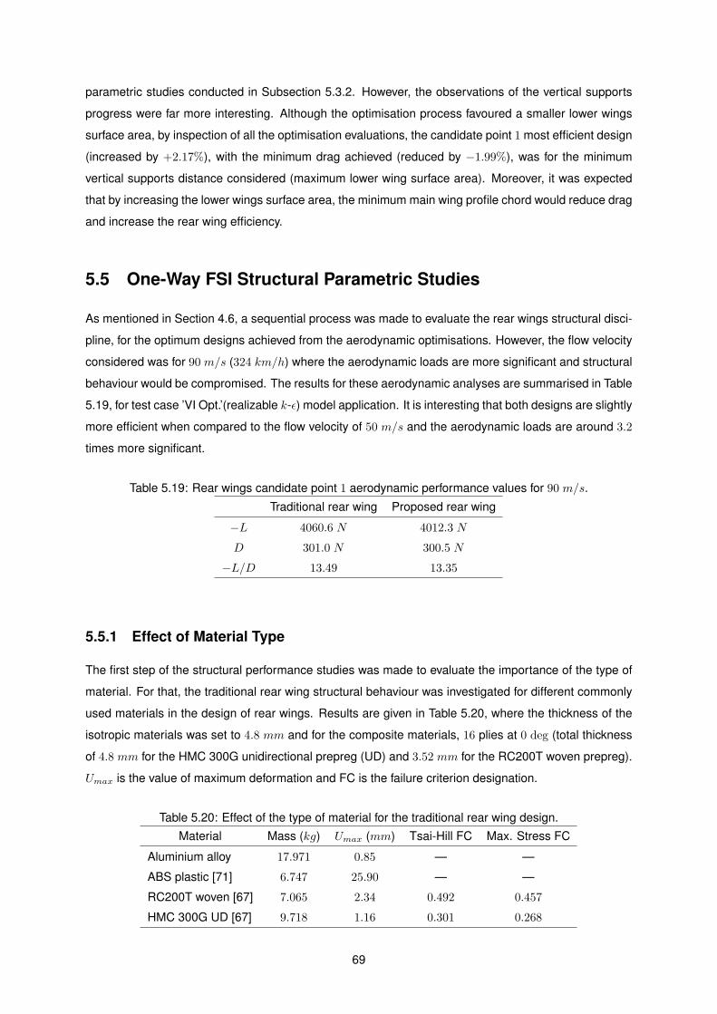
parametric studies conducted in Subsection 5.3.2. However, the observations of the vertical supports

progress were far more interesting. Although the optimisation process favoured a smaller lower wings

surface area, by inspection of all the optimisation evaluations, the candidate point 1 most efficient design

(increased by +2.17%), with the minimum drag achieved (reduced by −1.99%), was for the minimum

vertical supports distance considered (maximum lower wing surface area). Moreover, it was expected

that by increasing the lower wings surface area, the minimum main wing profile chord would reduce drag

and increase the rear wing efficiency.

5.5 One-Way FSI Structural Parametric Studies

As mentioned in Section 4.6, a sequential process was made to evaluate the rear wings structural disci-

pline, for the optimum designs achieved from the aerodynamic optimisations. However, the flow velocity

considered was for 90 m/s (324 km/h) where the aerodynamic loads are more significant and structural

behaviour would be compromised. The results for these aerodynamic analyses are summarised in Table

5.19, for test case ’VI Opt.’(realizable k-ǫ) model application. It is interesting that both designs are slightly

more efficient when compared to the flow velocity of 50 m/s and the aerodynamic loads are around 3.2

times more significant.

Table 5.19: Rear wings candidate point 1 aerodynamic performance values for 90 m/s.


−L 4060.6 N 4012.3 N

D 301.0 N 300.5 N

−L/D 13.49 13.35

5.5.1 Effect of Material Type

The first step of the structural performance studies was made to evaluate the importance of the type of

material. For that, the traditional rear wing structural behaviour was investigated for different commonly

used materials in the design of rear wings. Results are given in Table 5.20, where the thickness of the

isotropic materials was set to 4.8 mm and for the composite materials, 16 plies at 0 deg (total thickness

of 4.8 mm for the HMC 300G unidirectional prepreg (UD) and 3.52 mm for the RC200T woven prepreg).

Umax is the value of maximum deformation and FC is the failure criterion designation.

Table 5.20: Effect of the type of material for the traditional rear wing design.

Material Mass (kg) Umax (mm) Tsai-Hill FC Max. Stress FC

Aluminium alloy 17.971 0.85 — —

ABS plastic [71] 6.747 25.90 — —

RC200T woven [67] 7.065 2.34 0.492 0.457

HMC 300G UD [67] 9.718 1.16 0.301 0.268

69

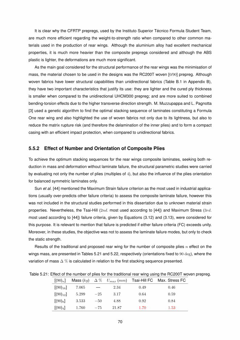
It is clear why the CFRTP prepregs, used by the Instituto Superior Tecnico Formula Student Team,

are much more efficient regarding the weight-to-strength ratio when compared to other common ma-

terials used in the production of rear wings. Although the aluminium alloy had excellent mechanical

properties, it is much more heavier than the composite prepregs considered and although the ABS

plastic is lighter, the deformations are much more significant.

As the main goal considered for the structural performance of the rear wings was the minimisation of

mass, the material chosen to be used in the designs was the RC200T woven [0/90] prepreg. Although

woven fabrics have lower structural capabilities than unidirectional fabrics (Table B.1 in Appendix B),

they have two important characteristics that justify its use: they are lighter and the cured ply thickness

is smaller when compared to the unidirectional UHCM300 prepreg; and are more suited to combined

bending-torsion effects due to the higher transverse direction strength. M. Muzzupappa and L. Pagnotta

[3] used a genetic algorithm to find the optimal stacking sequence of laminates constituting a Formula

One rear wing and also highlighted the use of woven fabrics not only due to its lightness, but also to

reduce the matrix rupture risk (and therefore the delamination of the inner plies) and to form a compact

casing with an efficient impact protection, when compared to unidirectional fabrics.

5.5.2 Effect of Number and Orientation of Composite Plies

To achieve the optimum stacking sequences for the rear wings composite laminates, seeking both re-

duction in mass and deformation without laminate failure, the structural parametric studies were carried

by evaluating not only the number of plies (multiples of 4), but also the influence of the plies orientation

for balanced symmetric laminates only.

Sun et al. [44] mentioned the Maximum Strain failure criterion as the most used in industrial applica-

tions (usually over-predicts other failure criteria) to assess the composite laminate failure, however this

was not included in the structural studies performed in this dissertation due to unknown material strain

properties. Nevertheless, the Tsai-Hill (2nd. most used according to [44]) and Maximum Stress (3rd.

most used according to [44]) failure criteria, given by Equations (3.12) and (3.13), were considered for

this purpose. It is relevant to mention that failure is predicted if either failure criteria (FC) exceeds unity.

Moreover, in these studies, the objective was not to assess the laminate failure modes, but only to check

the static strength.

Results of the traditional and proposed rear wing for the number of composite plies n effect on the

wings mass, are presented in Tables 5.21 and 5.22, respectively (orientations fixed to 90 deg), where the

variation of mass ∆ % is calculated in relation to the first stacking sequence presented.

Table 5.21: Effect of the number of plies for the traditional rear wing using the RC200T woven prepreg.

[(90)n] Mass (kg) ∆ % Umax (mm) Tsai-Hill FC Max. Stress FC

[(90)16] 7.065 — 2.34 0.49 0.46

[(90)12] 5.299 −25 3.17 0.64 0.59

[(90)8] 3.533 −50 4.88 0.92 0.84

[(90)4] 1.760 −75 21.87 1.70 1.53

70

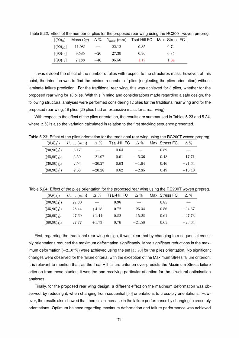
Table 5.22: Effect of the number of plies for the proposed rear wing using the RC200T woven prepreg.

[(90)n] Mass (kg) ∆ % Umax (mm) Tsai-Hill FC Max. Stress FC

[(90)20] 11.981 — 22.12 0.85 0.74

[(90)16] 9.585 −20 27.30 0.96 0.85

[(90)12] 7.188 −40 35.56 1.17 1.04

It was evident the effect of the number of plies with respect to the structures mass, however, at this

point, the intention was to find the minimum number of plies (neglecting the plies orientation) without

laminate failure prediction. For the traditional rear wing, this was achieved for 8 plies, whether for the

proposed rear wing for 16 plies. With this in mind and considerations made regarding a safe design, the

following structural analyses were performed considering 12 plies for the traditional rear wing and for the

proposed rear wing, 16 plies (20 plies had an excessive mass for a rear wing).

With respect to the effect of the plies orientation, the results are summarised in Tables 5.23 and 5.24,

where ∆ % is also the variation calculated in relation to the first stacking sequence presented.

Table 5.23: Effect of the plies orientation for the traditional rear wing using the RC200T woven prepreg.

[(θ,θ)3]s Umax (mm) ∆ % Tsai-Hill FC ∆ % Max. Stress FC ∆ %

[(90,90)3]s 3.17 — 0.64 — 0.59 —

[(45,90)3]s 2.50 −21.07 0.61 −5.36 0.48 −17.71

[(30,90)3]s 2.53 −20.27 0.63 −1.64 0.46 −21.64

[(60,90)3]s 2.53 −20.28 0.62 −2.85 0.49 −16.40

Table 5.24: Effect of the plies orientation for the proposed rear wing using the RC200T woven prepreg.

[(θ,θ)4]s Umax (mm) ∆ % Tsai-Hill FC ∆ % Max. Stress FC ∆ %

[(90,90)4]s 27.30 — 0.96 — 0.85 —

[(45,90)4]s 28.44 +4.18 0.72 −25.34 0.56 −34.67

[(30,90)4]s 27.69 +1.44 0.82 −15.28 0.61 −27.73

[(60,90)4]s 27.77 +1.73 0.76 −21.58 0.65 −23.64

First, regarding the traditional rear wing design, it was clear that by changing to a sequential cross-

ply orientations reduced the maximum deformation significantly. More significant reductions in the max-

imum deformation (−21.07%) were achieved using the set [45,90] for the plies orientation. No significant

changes were observed for the failure criteria, with the exception of the Maximum Stress failure criterion.

It is relevant to mention that, as the Tsai-Hill failure criterion over-predicts the Maximum Stress failure

criterion from these studies, it was the one receiving particular attention for the structural optimisation

analyses.

Finally, for the proposed rear wing design, a different effect on the maximum deformation was ob-

served, by reducing it, when changing from sequential [90] orientations to cross-ply orientations. How-

ever, the results also showed that there is an increase in the failure performance by changing to cross-ply

orientations. Optimum balance regarding maximum deformation and failure performance was achieved

71

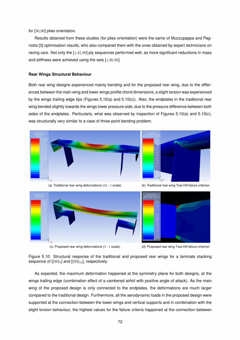
for [30,90] plies orientation.

Results obtained from these studies (for plies orientation) were the same of Muzzupappa and Pag-

notta [3] optimisation results, who also compared them with the ones obtained by expert technicians on

racing cars. Not only the [±45,90] ply sequences performed well, as more significant reductions in mass

and stiffness were achieved using the sets [±30,90].

Rear Wings Structural Behaviour

Both rear wing designs experienced mainly bending and for the proposed rear wing, due to the differ-

ences between the main wing and lower wings profile chord dimensions, a slight torsion was experienced

by the wings trailing edge tips (Figures 5.10(a) and 5.10(c)). Also, the endplates in the traditional rear

wing bended slightly towards the wings lower pressure side, due to the pressure difference between both

sides of the endplates. Particularly, what was observed by inspection of Figures 5.10(a) and 5.10(c),

was structurally very similar to a case of three-point bending problem.

(a) Traditional rear wing deformations (10 : 1 scale). (b) Traditional rear wing Tsai-Hill failure criterion.

(c) Proposed rear wing deformations (5 : 1 scale). (d) Proposed rear wing Tsai-Hill failure cirterion.

Figure 5.10: Structural response of the traditional and proposed rear wings for a laminate stacking

sequence of [(90)8] and [(90)16], respectively.

As expected, the maximum deformation happened at the symmetry plane for both designs, at the

wings trailing edge (combination effect of a cambered airfoil with positive angle of attack). As the main

wing of the proposed design is only connected to the endplates, the deformations are much larger

compared to the traditional design. Furthermore, all the aerodynamic loads in the proposed design were

supported at the connection between the lower wings and vertical supports and in combination with the

slight torsion behaviour, the highest values for the failure criteria happened at the connection between

72

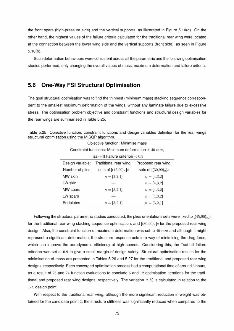
the front spars (high-pressure side) and the vertical supports, as illustrated in Figure 5.10(d). On the

other hand, the highest values of the failure criteria calculated for the traditional rear wing were located

at the connection between the lower wing side and the vertical supports (front side), as seen in Figure

5.10(b).

Such deformation behaviours were consistent across all the parametric and the following optimisation

studies performed, only changing the overall values of mass, maximum deformation and failure criteria.

5.6 One-Way FSI Structural Optimisation

The goal structural optimisation was to find the thinnest (minimum mass) stacking sequence correspon-

dent to the smallest maximum deformation of the wings, without any laminate failure due to excessive

stress. The optimisation problem objective and constraint functions and structural design variables for

the rear wings are summarised in Table 5.25.

Table 5.25: Objective function, constraint functions and design variables definition for the rear wings

structural optimisation using the MISQP algorithm.

Objective function: Minimise mass

Constraint functions: Maximum deformation < 40 mm,

Tsai-Hill Failure criterion < 0.9

Design variable:

Number of plies

Traditional rear wing:

sets of [(45,90)n]s

Proposed rear wing:

sets of [(30,90)n]s

MW skin n = [3,2,1] n = [4,3,2]

LW skin — n = [4,3,2]

MW spars n = [3,2,1] n = [4,3,2]

LW spars — n = [4,3,2]

Endplates n = [3,2,1] n = [3,2,1]

Following the structural parametric studies conducted, the plies orientations sets were fixed to [(45,90)n]s

for the traditional rear wing stacking sequence optimisation, and [(30,90)n]s for the proposed rear wing

design. Also, the constraint function of maximum deformation was set to 40 mm and although it might

represent a significant deformation, the structure response acts in a way of minimising the drag force,

which can improve the aerodynamic efficiency at high speeds. Considering this, the Tsai-hill failure

criterion was set at 0.9 to give a small margin of design safety. Structural optimisation results for the

minimisation of mass are presented in Tables 5.26 and 5.27 for the traditional and proposed rear wing

designs, respectively. Each converged optimisation process had a computational time of around 6 hours,

as a result of 25 and 74 function evaluations to conclude 6 and 12 optimisation iterations for the tradi-

tional and proposed rear wing designs, respectively. The variation ∆ % is calculated in relation to the

1st. design point.

With respect to the traditional rear wing, although the more significant reduction in weight was ob-

tained for the candidate point 2, the structure stiffness was significantly reduced when compared to the

73

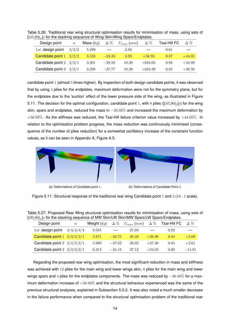
Table 5.26: Traditional rear wing structural optimisation results for minimisation of mass, using sets of

[(45,90)n]s for the stacking sequence of Wing Skin/Wing Spars/Endplates.

Design point n Mass (kg) ∆ % Umax (mm) ∆ % Tsai-Hill FC ∆ %

1st. design point 3/3/3 5.299 — 2.50 — 0.61 —

Candidate point 1 2/2/2 3.533 −33.33 3.93 +56.93 0.87 +44.05

Candidate point 2 2/2/1 3.201 −39.58 18.39 +634.63 0.88 +44.99

Candidate point 3 2/3/1 3.298 −37.77 18.39 +634.39 0.85 +40.50

candidate point 1 (almost 5 times higher). By inspection of both design candidate points, it was observed

that by using 4 plies for the endplates, maximum deformation were not for the symmetry plane, but for

the endplates due to the ’suction’ effect of the lower pressure side of the wing, as illustrated in Figure

5.11. The decision for the optimal configuration, candidate point 1, with 8 plies ([(45,90)2]s) for the wing

skin, spars and endplates, reduced the mass in −33.33% and increased the maximum deformation by

+56.93%. As the stiffness was reduced, the Tsai-Hill failure criterion value increased by +44.05%. In

relation to the optimisation problem progress, the mass reduction was continuously minimised (conse-

quence of the number of plies reduction) for a somewhat oscillatory increase of the constraint function

values, as it can be seen in Appendix A, Figure A.5.

(a) Deformations of Candidate point 1. (b) Deformations of Candidate Point 2.

Figure 5.11: Structural response of the traditional rear wing Candidate point 1 and 2 (10 : 1 scale).

Table 5.27: Proposed Rear Wing structural optimisation results for minimisation of mass, using sets of

[(30,90)n]s for the stacking sequence of MW Skin/LW Skin/MW Spars/LW Spars/Endplates.

Design point n Weight (kg) ∆ % Umax (mm) ∆ % Tsai-Hill FC ∆ %

1st. design point 4/4/4/4/4 9.585 — 27.69 — 0.82 —

Candidate point 1 3/3/2/2/1 5.871 −38.75 38.49 +38.98 0.84 +2.69

Candidate point 2 3/4/2/2/1 5.960 −37.82 38.02 +37.30 0.84 +2.61

Candidate point 3 3/3/3/2/1 6.313 −34.13 37.12 +34.03 0.69 −14.91

Regarding the proposed rear wing optimisation, the most significant reduction in mass and stiffness

was achieved with 12 plies for the main wing and lower wings skin, 8 plies for the main wing and lower

wings spars and 4 plies for the endplates components. The mass was reduced by −38.48% for a max-

imum deformation increase of +56.93% and the structural behaviour experienced was the same of the

previous structural analyses, explained in Subsection 5.5.2. It was also noted a much smaller decrease

in the failure performance when compared to the structural optimisation problem of the traditional rear

74

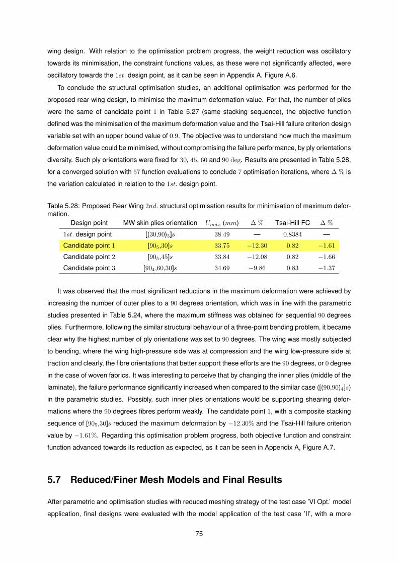
wing design. With relation to the optimisation problem progress, the weight reduction was oscillatory

towards its minimisation, the constraint functions values, as these were not significantly affected, were

oscillatory towards the 1st. design point, as it can be seen in Appendix A, Figure A.6.

To conclude the structural optimisation studies, an additional optimisation was performed for the

proposed rear wing design, to minimise the maximum deformation value. For that, the number of plies

were the same of candidate point 1 in Table 5.27 (same stacking sequence), the objective function

defined was the minimisation of the maximum deformation value and the Tsai-Hill failure criterion design

variable set with an upper bound value of 0.9. The objective was to understand how much the maximum

deformation value could be minimised, without compromising the failure performance, by ply orientations

diversity. Such ply orientations were fixed for 30, 45, 60 and 90 deg. Results are presented in Table 5.28,

for a converged solution with 57 function evaluations to conclude 7 optimisation iterations, where ∆ % is

the variation calculated in relation to the 1st. design point.

Table 5.28: Proposed Rear Wing 2nd. structural optimisation results for minimisation of maximum defor-

mation.

Design point MW skin plies orientation Umax (mm) ∆ % Tsai-Hill FC ∆ %

1st. design point [(30,90)3]s 38.49 — 0.8384 —

Candidate point 1 [905,30]s 33.75 −12.30 0.82 −1.61

Candidate point 2 [905,45]s 33.84 −12.08 0.82 −1.66

Candidate point 3 [904,60,30]s 34.69 −9.86 0.83 −1.37

It was observed that the most significant reductions in the maximum deformation were achieved by

increasing the number of outer plies to a 90 degrees orientation, which was in line with the parametric

studies presented in Table 5.24, where the maximum stiffness was obtained for sequential 90 degrees

plies. Furthermore, following the similar structural behaviour of a three-point bending problem, it became

clear why the highest number of ply orientations was set to 90 degrees. The wing was mostly subjected

to bending, where the wing high-pressure side was at compression and the wing low-pressure side at

traction and clearly, the fibre orientations that better support these efforts are the 90 degrees, or 0 degree

in the case of woven fabrics. It was interesting to perceive that by changing the inner plies (middle of the

laminate), the failure performance significantly increased when compared to the similar case ([(90,90)4]s)

in the parametric studies. Possibly, such inner plies orientations would be supporting shearing defor-

mations where the 90 degrees fibres perform weakly. The candidate point 1, with a composite stacking

sequence of [905,30]s reduced the maximum deformation by −12.30% and the Tsai-Hill failure criterion

value by −1.61%. Regarding this optimisation problem progress, both objective function and constraint

function advanced towards its reduction as expected, as it can be seen in Appendix A, Figure A.7.

5.7 Reduced/Finer Mesh Models and Final Results

After parametric and optimisation studies with reduced meshing strategy of the test case ’VI Opt.’ model

application, final designs were evaluated with the model application of the test case ’II’, with a more

75

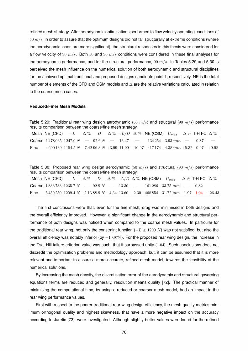
refined mesh strategy. After aerodynamic optimisations performed to flow velocity operating conditions of

50 m/s, in order to assure that the optimum designs did not fail structurally at extreme conditions (where

the aerodynamic loads are more significant), the structural responses in this thesis were considered for

a flow velocity of 90 m/s. Both 50 and 90 m/s conditions were considered in these final analyses for

the aerodynamic performance, and for the structural performance, 90 m/s. In Tables 5.29 and 5.30 is

perceived the mesh influence on the numerical solution of both aerodynamic and structural disciplines

for the achieved optimal traditional and proposed designs candidate point 1, respectively. NE is the total

number of elements of the CFD and CSM models and ∆ are the relative variations calculated in relation

to the coarse mesh cases.

Reduced/Finer Mesh Models

Table 5.29: Traditional rear wing design aerodynamic (50 m/s) and structural (90 m/s) performance

results comparison between the coarse/fine mesh strategy.

Mesh NE (CFD) −L ∆ % D ∆ % −L/D ∆ % NE (CSM) Umax ∆ % T-H FC ∆ %

Coarse 1 478 035 1247.0 N — 92.6 N — 13.47 — 134 254 3.93 mm — 0.87 —

Fine 4 600 139 1154.5 N −7.42 96.3 N +3.99 11.99 −10.97 417 174 4.38 mm +5.32 0.97 +9.98

Table 5.30: Proposed rear wing design aerodynamic (50 m/s) and structural (90 m/s) performance

results comparison between the coarse/fine mesh strategy.

Mesh NE (CFD) −L ∆ % D ∆ % −L/D ∆ % NE (CSM) Umax ∆ % T-H FC ∆ %

Coarse 1 833 733 1235.7 N — 92.9 N — 13.30 — 161 286 33.75 mm — 0.82 —

Fine 5 450 250 1209.4 N −2.13 88.9 N −4.34 13.60 +2.30 468 854 31.72 mm −1.97 1.04 +26.43

The first conclusions were that, even for the fine mesh, drag was minimised in both designs and

the overall efficiency improved. However, a significant change in the aerodynamic and structural per-

formance of both designs was noticed when compared to the coarse mesh values. In particular for

the traditional rear wing, not only the constraint function (−L ≥ 1200 N ) was not satisfied, but also the

overall efficiency was notably inferior (by −10.97%). For the proposed rear wing design, the increase in

the Tsai-Hill failure criterion value was such, that it surpassed unity (1.04). Such conclusions does not

discredit the optimisation problems and methodology approach, but, it can be assumed that it is more

relevant and important to assure a more accurate, refined mesh model, towards the feasibility of the

numerical solutions.

By increasing the mesh density, the discretisation error of the aerodynamic and structural governing

equations terms are reduced and generally, resolution means quality [72]. The practical manner of

minimising the computational time, by using a reduced or coarser mesh model, had an impact in the

rear wing performance values.

First with respect to the poorer traditional rear wing design efficiency, the mesh quality metrics min-

imum orthogonal quality and highest skewness, that have a more negative impact on the accuracy

according to Juretic [73], were investigated. Although slightly better values were found for the refined

76

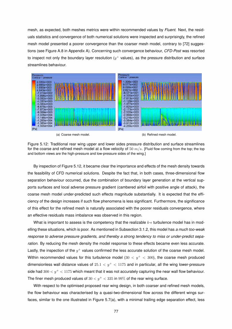
mesh, as expected, both meshes metrics were within recommended values by Fluent. Next, the resid-

uals statistics and convergence of both numerical solutions were inspected and surprisingly, the refined

mesh model presented a poorer convergence than the coarser mesh model, contrary to [72] sugges-

tions (see Figure A.8 in Appendix A). Concerning such convergence behaviour, CFD-Post was resorted

to inspect not only the boundary layer resolution (y+ values), as the pressure distribution and surface

streamlines behaviour.

(a) Coarse mesh model. (b) Refined mesh model.

Figure 5.12: Traditional rear wing upper and lower sides pressure distribution and surface streamlines

for the coarse and refined mesh model at a flow velocity of 50 m/s. [Fluid flow coming from the top; the top

and bottom views are the high-pressure and low-pressure sides of the wing.]

By inspection of Figure 5.12, it became clear the importance and effects of the mesh density towards

the feasibility of CFD numerical solutions. Despite the fact that, in both cases, three-dimensional flow

separation behaviour occurred, due the combination of boundary layer generation at the vertical sup-

ports surfaces and local adverse pressure gradient (cambered airfoil with positive angle of attack), the

coarse mesh model under-predicted such effects magnitude substantially. It is expected that the effi-

ciency of the design increases if such flow phenomena is less significant. Furthermore, the significance

of this effect for the refined mesh is naturally associated with the poorer residuals convergence, where

an effective residuals mass imbalance was observed in this region.

What is important to assess is the competency that the realizable k-ǫ turbulence model has in mod-

elling these situations, which is poor. As mentioned in Subsection 3.1.2, this model has a much too-weak

response to adverse pressure gradients, and thereby a strong tendency to miss or under-predict sepa-

ration. By reducing the mesh density the model response to these effects became even less accurate.

Lastly, the inspection of the y+ values confirmed the less accurate solution of the coarse mesh model.

Within recommended values for this turbulence model (30 < y+ < 300), the coarse mesh produced

dimensionless wall distance values of 25.1 < y+ < 1175 and in particular, all the wing lower-pressure

side had 300 < y+ < 1175 which meant that it was not accurately capturing the near wall flow behaviour.

The finer mesh produced values of 30 < y+ < 335 in 99% of the rear wing surface.

With respect to the optimised proposed rear wing design, in both coarser and refined mesh models,

the flow behaviour was characterised by a quasi-two-dimensional flow across the different wings sur-

faces, similar to the one illustrated in Figure 5.7(a), with a minimal trailing edge separation effect, less

77

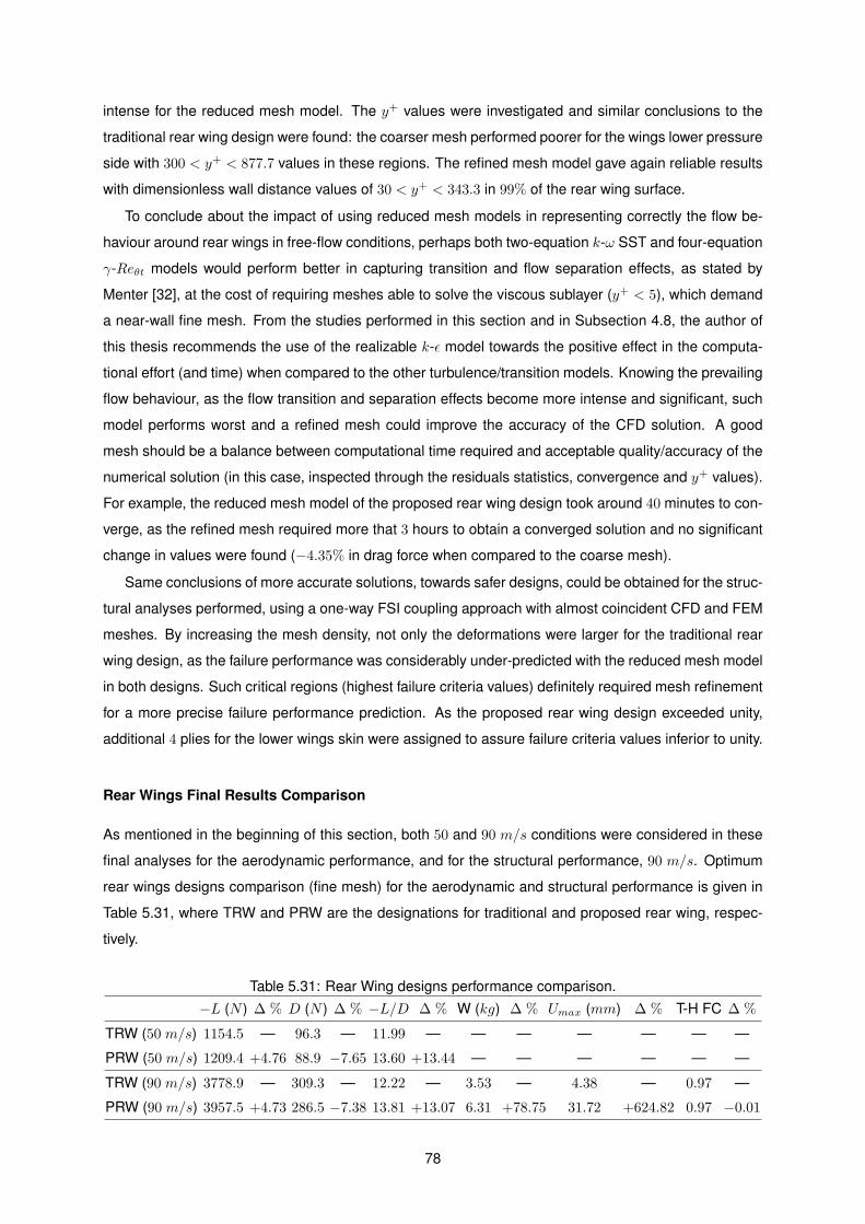
intense for the reduced mesh model. The y+ values were investigated and similar conclusions to the

traditional rear wing design were found: the coarser mesh performed poorer for the wings lower pressure

side with 300 < y+ < 877.7 values in these regions. The refined mesh model gave again reliable results

with dimensionless wall distance values of 30 < y+ < 343.3 in 99% of the rear wing surface.

To conclude about the impact of using reduced mesh models in representing correctly the flow be-

haviour around rear wings in free-flow conditions, perhaps both two-equation k-ω SST and four-equation

γ-Reθt models would perform better in capturing transition and flow separation effects, as stated by

Menter [32], at the cost of requiring meshes able to solve the viscous sublayer (y+ < 5), which demand

a near-wall fine mesh. From the studies performed in this section and in Subsection 4.8, the author of

this thesis recommends the use of the realizable k-ǫ model towards the positive effect in the computa-

tional effort (and time) when compared to the other turbulence/transition models. Knowing the prevailing

flow behaviour, as the flow transition and separation effects become more intense and significant, such

model performs worst and a refined mesh could improve the accuracy of the CFD solution. A good

mesh should be a balance between computational time required and acceptable quality/accuracy of the

numerical solution (in this case, inspected through the residuals statistics, convergence and y+ values).

For example, the reduced mesh model of the proposed rear wing design took around 40 minutes to con-

verge, as the refined mesh required more that 3 hours to obtain a converged solution and no significant

change in values were found (−4.35% in drag force when compared to the coarse mesh).

Same conclusions of more accurate solutions, towards safer designs, could be obtained for the struc-

tural analyses performed, using a one-way FSI coupling approach with almost coincident CFD and FEM

meshes. By increasing the mesh density, not only the deformations were larger for the traditional rear

wing design, as the failure performance was considerably under-predicted with the reduced mesh model

in both designs. Such critical regions (highest failure criteria values) definitely required mesh refinement

for a more precise failure performance prediction. As the proposed rear wing design exceeded unity,

additional 4 plies for the lower wings skin were assigned to assure failure criteria values inferior to unity.

Rear Wings Final Results Comparison

As mentioned in the beginning of this section, both 50 and 90 m/s conditions were considered in these

final analyses for the aerodynamic performance, and for the structural performance, 90 m/s. Optimum

rear wings designs comparison (fine mesh) for the aerodynamic and structural performance is given in

Table 5.31, where TRW and PRW are the designations for traditional and proposed rear wing, respec-

tively.

Table 5.31: Rear Wing designs performance comparison.

−L (N ) ∆ % D (N ) ∆ % −L/D ∆ % W (kg) ∆ % Umax (mm) ∆ % T-H FC ∆ %

TRW (50 m/s) 1154.5 — 96.3 — 11.99 — — — — — — —

PRW (50 m/s) 1209.4 +4.76 88.9 −7.65 13.60 +13.44 — — — — — —

TRW (90 m/s) 3778.9 — 309.3 — 12.22 — 3.53 — 4.38 — 0.97 —

PRW (90 m/s) 3957.5 +4.73 286.5 −7.38 13.81 +13.07 6.31 +78.75 31.72 +624.82 0.97 −0.01

78

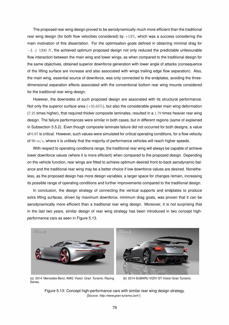
The proposed rear wing design proved to be aerodynamically much more efficient than the traditional

rear wing design (for both flow velocities considered) by +13%, which was a success considering the

main motivation of this dissertation. For the optimisation goals defined in obtaining minimal drag for

−L ≥ 1200 N , the achieved optimum proposed design not only reduced the predictable unfavourable

flow interaction between the main wing and lower wings, as when compared to the traditional design for

the same objectives, obtained superior downforce generation with lower angle of attacks (consequence

of the lifting surface are increase and also associated with wings trailing edge flow separation). Also,

the main wing, essential source of downforce, was only connected to the endplates, avoiding the three-

dimensional separation effects associated with the conventional bottom rear wing mounts considered

for the traditional rear wing design.

However, the downsides of such proposed design are associated with its structural performance.

Not only the superior surface area (+35.65%), but also the considerable greater main wing deformation

(7.25 times higher), that required thicker composite laminates, resulted in a 1.79 times heavier rear wing

design. The failure performances were similar in both cases, but in different regions (same of explained

in Subsection 5.5.2). Even though composite laminate failure did not occurred for both designs, a value

of 0.97 is critical. However, such values were simulated for critical operating conditions, for a flow velocity

of 90 m/s, where it is unlikely that the majority of performance vehicles will reach higher speeds.

With respect to operating conditions range, the traditional rear wing will always be capable of achieve

lower downforce values (where it is more efficient) when compared to the proposed design. Depending

on the vehicle function, rear wings are fitted to achieve optimum desired front-to-back aerodynamic bal-

ance and the traditional rear wing may be a better choice if low downforce values are desired. Nonethe-

less, as the proposed design has more design variables, a larger space for changes remain, increasing

its possible range of operating conditions and further improvements compared to the traditional design.

In conclusion, the design strategy of connecting the vertical supports and endplates to produce

extra lifting surfaces, driven by maximum downforce, minimum drag goals, was proven that it can be

aerodynamically more efficient than a traditional rear wing design. Moreover, it is not surprising that

in the last two years, similar design of rear wing strategy has been introduced in two concept high-

performance cars as seen in Figure 5.13.

(a) 2014 Mercedes-Benz AMG Vision Gran Turismo RacingSeries.

(b) 2014 SUBARU VIZIV GT Vision Gran Turismo.

Figure 5.13: Concept high-performance cars with similar rear wing design strategy.

[Source: http://www.gran-turismo.com/ ]

79

Chapter 6

Conclusions

The purpose of this thesis was to develop knowledge in the field of high-performance automobile aero-

dynamic devices, in particular rear wings, which have crucial effects on vehicles performance. Such

expertise was focused on the comparison of two different design strategies. A traditional design, gener-

ally seen in high-performance applications, and a proposed one, where the surface connection between

the endplates and vertical supports is used to create additional downforce. A further motivation was

the fact that the author did not found information covering the proposed design strategy in the published

literature. Rear wings cover two core disciplines, aerodynamics and structures, and these were the ob-

jectives of this thesis, establish a multidisciplinary design analysis and optimisation procedure to assess

aero-structural performance of aerodynamic these devices.

6.1 Analyses Conclusions and Recommendations

From the studies performed in this thesis, a MDAO process for optimal preliminary design was devel-

oped for rear wings, but it can also be applied to any other automotive aerodynamic components. As

in almost every high-performance vehicles manufacturers, the use of CAE tools (here ANSYS R© Work-

bench) proved to be an efficient simulation platform to assure multidisciplinary synergy (CFD, CSM, FSI

and optimisation) towards feasible products in a relatively short time frame.

Prior to perform any device design, knowledge of the general (or specific) operating conditions, and to

which vehicle it is being applied is required. Effectiveness of the aerodynamic performance should be the

focus during the design procedure. After the definition of the design variables and functions of interest,

concerns should be taken regarding the CFD model. Verification of both mesh models and turbulence

modelling strategy is extremely important. Fine meshes along with transition models drives improved

accuracy of the numerical solution at the cost of computational time. Coarse meshes with turbulence

models can lead to accuracy compromise. Even though, in this thesis, the use of the realizable k-ǫ

turbulence model (with non-equilibrium wall functions) with relative coarse meshes (around two million

elements) proved to be a good trade-off regarding computational effort and solution accuracy, as long

as no complex three-dimensional flow behaviours are expected. Aerodynamic parametric studies of

81

the design variables influence the optimisation computational time by focusing on the most impacting

variables to obtain optimal designs, leading to a lower number of optimisation iterations.

Regarding the structural discipline, optimised performance can be obtained from proper shape de-

signs by means of fluid-structure interaction in order to obtain minimum mass and deformations. Fur-

thermore, if small deformations are expected and aero-elasticity phenomena could be disregarded, a

one-way coupling technique has significant computational advantages. Structural efficiency can be

obtained by selecting materials with high strength-to-weight, such as CFRTP. The structure effective-

ness should be assessed for critical, or extreme operating conditions, where failure performance can

be compromised. Again, parametric studies of the structural design variables of interest leverage the

optimisation procedure, towards fast achievement of optimal structural attributes.

For both aerodynamic and structural disciplines optimisation, the implementation of sequential quadratic

programming (SQP) methods, the NLQPL and the MISQP optimisers respectively for continuous (aero-

dynamic discipline) and discrete (structural discipline) parameters, proved to be an efficient choice re-

garding the design improvements and computational time to accomplish converged solutions.

6.2 Future Work

Prior to perform any scale-model wind tunnel validation work of the rear wings designed in this thesis,

further CFD analyses should be performed regarding improved accuracy of numerical solutions.

If computational resources would not be an obstacle, a specific vehicle should be designated to be

equipped with optimal rear wing designs along with further refined dissertation methodology application.

The results presented in this thesis were achieved considering steady-state/static conditions with a

hybrid mesh strategy (relatively coarse) and minimal oscillatory converged (CFD) solutions were no-

ticed. Although such approach in developing a reduced mesh model had significant computational time

advantages, a search for improved accuracy solutions should consider transient analyses with a more

accurate fully structured meshing strategy.

Also, multi-objective aerodynamic and structural optimisation problem considering two-way FSI ap-

proach with more design variables should be considered to explore the maximum efficiency possible

across determined range of operating conditions (different velocities and for yawed conditions). Not only

wing profile chord variation along wingspan could be investigated, but also twisting effects and specific

aerodynamic goals to achieve desired front-to-rear aerodynamic balance.

Finally, within budget conditions, scale-models of the optimum rear wings and vehicle should be

manufactured to validate optimum designs with wind-tunnel data.

82

Bibliography

[1] J. Katz. Race Car Aerodynamics: Designing for Speed. Bentley Publishers, 1995. ISBN 0-8376-

0142-8.

[2] Understanding f1 racing: Aerodynamics. https://www.formula1.com/content/fom-website/en/

championship/inside-f1/understanding-f1-racing/Aerodynamics.html, 2015. Acessed on

December 2015.

[3] M. Muzzupappa and L. Pagnotta. Optimum design of a formula one rear wing using a genetic

algorithm. In D. Marjanovic, editor, 7th International Design Conference, DESIGN, pages 1217–

1222, Dubrovnik-Cavta, Croatia, 2002. ISBN 953-6313-45-6.

[4] J. N. Reddy. Mechanics of Laminated Composite Plates and Shells - Theory and Analysis. CRC

Press, 2nd edition, 2004. ISBN 0-8493-1592-1.

[5] P. Wright. Formula 1 Technology. Premiere Series Books. Society of Automotive Engineers Inc,

2001. ISBN 978-0768002348.

[6] A. Shedden. The design and optimisation of an aerodynamic package for an Aston Martin V8

Vantage eligible to complete in the Britcar championship. Master thesis in motorsport engineering,

Oxford Brookes University, August 2010.

[7] S. McBeath. Rear wing rudiments. Racecar Enginnering, 25(12):52–58, December 2015.

[8] S. McBeath. Competition Car Aerodynamics. Haynes Publishing, 2nd edition, 2006. ISBN 978-

0857330079.

[9] S. McBeath. How high? Racecar Enginnering, 17(9):19–20, September 2007.

[10] R. Aiguabella. Formula one rear wing optimization. Master thesis in motorsport engineering,

METCA, collaboration between Epsilon Euskadi and Mondragon Unibertsitatea, December 2010.

[11] C. Casiraghi. Race Car Aerodynamics, Royal Institute of Technology. http://www2.mech.kth.se/

courses/5C1211/Casiraghi_2010.pdf, 2010. Acessed on December 2015.

[12] M. J. Fuller. A brief history of sports car racing. http://www.mulsannescorner.com/history.html,

1996. Acessed on December 2015.

83

https://www.formula1.com/content/fom-website/en/championship/inside-f1/understanding-f1-racing/Aerodynamics.html

https://www.formula1.com/content/fom-website/en/championship/inside-f1/understanding-f1-racing/Aerodynamics.html

http://www2.mech.kth.se/courses/5C1211/Casiraghi_2010.pdf

http://www2.mech.kth.se/courses/5C1211/Casiraghi_2010.pdf

http://www.mulsannescorner.com/history.html

[13] Allianz. Evolution of aerodynamics. http://www.f1network.net/main/s107/st22394.htm, 2003.

Acessed on December 2015.

[14] J. Katz. Aerodynamics of race cars. Annual Review of Fluid Mechanics, 38:27–63, 2006. doi:

10.1146/annurev.fluid.38.050304.092016.

[15] J. Zerihan and X. Zhang. Aerodynamics of a single element wing in ground effect. Journal of

Aircraft, 37(6):1058–1064, 2000. doi: 10.2514/2.2711.

[16] J. Wiedemann. Some basic investigations into the principles of ground simulation techniques in

automotive wind tunnels. Technical Report 890369, SAE International, 1989. doi: 10.4271/890369.

[17] C. Coulliette and A. Plotkin. Airfoil ground effect revisited. In 13th Applied Aerodynamics Confer-

ence, 1995. doi: 10.2514/6.1995-1832. San Diego, CA, USA.

[18] J. Katz. Calculation of the aerodynamic forces on automotive lifting surfaces. Journal of Fluids

Engineering, 107(4):438–443, 1985. doi: 10.1115/1.3242507.

[19] R. B. Sharma and R. Bansal. Cfd simulation for flow over passenger car using tail plates for

aerodynamic drag reduction. IOSR Journal of Mechanical and Civil Engineering, 7(5):28–35, 2013.

[20] E. L. Houghton and P. W. Carpenter. Aerodynamics for Engineering Students. Butterworth-

Heinemann, 5th edition, 2003. ISBN 0-7506-5111-3.

[21] J. Katz and R. Largman. Experimental study of the aerodynamic interaction between an enclosed-

wheel racing-car and its rear wing. Journal of Fluids Engineering, 111(2):154–159, 1989. doi:

10.1115/1.3243616.

[22] J. Katz and L. Dykstra. Effect of wing/body interaction on the aerodynamics of two generic racing

cars. Technical Report 920349, SAE International, 1992. doi: 10.4271/920349.

[23] S. Wordley and J. Saunders. Aerodynamics for formula sae: A numerical, wind tunnel and on-track

study. Technical Report 2006-01-0808, SAE International, 2006. doi: 10.4271/2006-01-0808.

[24] J. Katz and R. Largman. Effect of 90 degree flap on the aerodynamics of a two-element airfoil.

Journal of Fluids Engineering, 111(1):93–94, 1989. doi: 10.1115/1.3243605.

[25] R. Myose, M. Papadakis, and I. Heron. Gurney flap experiments on airfoils, wings and reflection

plane model. Journal of Aircraft, 35(2):206–211, 1998. doi: 10.2514/2.2309.

[26] R. K. Hanna. CFD in sport - a retrospective; 1992 - 2012. Procedia Engineering, 34(6):622–627,

2012. doi: 10.1016/j.proeng.2012.04.106.

[27] K. R. Laflin, S. M. Klauzmeyer, T. Zickuhr, et al. Data summary from second AIAA computational

fluid dynamics drag prediction workshop. Journal of Aircraft, 42(5):1165–1178, 2005.

[28] J. C. Vassberg, E. N. Tinoco, M. Mani, et al. Summary of the forth aiaa computational fluid dynamics

drag prediction workshop. Journal of Aircraft, 51(4):1070–1089, 2014. doi: 10.2514/1.C032418.

84

http://www.f1network.net/main/s107/st22394.htm

[29] D. W. Levy, K. R. Laflin, E. N. Tinoco, et al. Summary of data from the fifth AIAA CFD drag prediction

workshop. In 51st AIAA Aerospace Sciences Meeting. Aerospace Sciences Meetings, 2013. doi:

10.2514/6.2013-46. Orlando, FL, USA.

[30] J. John D. Anderson. Fundamentals of Aerodynamics. McGraw-Hill Series in Aeronautical and

Aerospace Engineering, 5th edition, 2010. ISBN 978-0-07-339810-5.

[31] ANSYS R© FLUENT Theory Guide. ANSYS R©, Inc., 2012. Release 14.5.

[32] F. R. Menter. Turbulence modeling for engineering flows. Technical report, ANSYS, Inc., 2011. A

Technical Paper from ANSYS, Inc.

[33] D. C. Wilcox. Turbulence Modeling for CFD. DCW Industries, Inc., 2th edition, 1998.

[34] J. Kesti and S. Olsson. Fluid structure interaction analysis on the aerodynamic performance of

underbody panels. Master thesis in fluid and solid mechanics, Chalmers Univerity of Technology,

2014.

[35] A. el Quazizi. CFD based aerodynamic redesign of a Marcos LM600. Master thesis in aerospace

engineering, Delft Univerity of Technology, 2006.

[36] J. Keogh, G. Doig, and S. Diasinos. The influence of compressibility effects in correlation issues for

aerodynamic development of racing cars. In Proceedings of the 18th Australasian Fluid Mechanics

Conference, pages 1–4, December 2012. ISBN 9780646583730. Launceston, Australia.

[37] E. Canada. Aerodynamic analysis and optimisation of the rear wing of a WRC car. Master thesis

in motorsport engineering, Oxford Brookes University, September 2012.

[38] J. Cederlund and J. Vikstrom. The aerodynamic influence of rim design on a sports car and its

interaction with the wing and disffuser flow. Master thesis in automotive engineering, Chalmers

Univerity of Technology, 2010.

[39] A. Humunic and G. Humunic. CFD investigations of an open-wheel race car. In 4th European

Automotive Simulation Conference, pages 85–94. ANSYS, Inc., July 2009. Munich, Germany.

[40] F. R. Menter. Two-equation eddy-viscosity turbulence models for engineering applications. AIAA

Journal, 32(8):1598–1605, 1994. doi: 10.2514/3.12149.

[41] F.-K. Benra, H. Dohmen, J. Pei, S. Shuster, and B. Wan. A comparison of one-way and two-

way coupling methods for numerical analysis of fluid-structure interactions. Journal of Applied

Mathematics, 2011. doi: 10.1155/2011/853560. Volume 2011, Article ID 853560, 16 pages.

[42] ANSYS R© Mechanical User’s Guide. ANSYS R©, Inc., 2012. Release 14.5.

[43] D. Roylance. Laminated composite plates. Technical Report MA 02139, Massachusetts Institute of

Technology, 2000.

85

[44] C. Sun, B. Quinn, T. J., D. Oplinger, and W. Hughes. Comparative evaluation of failure analy-

sis methods for composite laminates. Technical Report DOT/FAA/AR-95/109, U.S. Department

of Transportation, Federal Aviation Administration, Office of Aviation Research, Washington, D.C.

20591, May 1996.

[45] W. Q. Wang and Y. Yan. Strongly coupling of partitioned fluid/solid interaction solvers using reduced-

order models. Applied Mathematical Modelling, 34(12):3817–3830, 2010. doi: 10.1016/j.apm.2010.

03.022.

[46] T. Richter. Numerical methods for fluid-structure interaction problems, universitat hei-

delberg. https://www.researchgate.net/publication/228692330_Numerical_Methods_for_

Fluid-Structure_Interaction_Problems, August 2010. Acessed on February 2016.

[47] G. Hou, J. Wang, and A. Layton. Numerical methods for fluid-structure interaction - a review. Com-

munications in Computational Physics, 12(2):337–377, August 2012. doi: 10.4208/cicp.291210.

290411s.

[48] A. D. Boer, H. Bijl, and A. Zuijlen. Comparing different methods for the coupling of non-matching

meshes in fluid-structure interaction computations. In 17th AIAA Computational Fluid Dynamics

Conference, 2005. doi: 10.2514/6.2005-4620. Toronto, Ontario, Canada.

[49] J. M. Vassen, P. DeVincenzo, C. Hirsch, and B. Leonard. Strong coupling algorithm to solve fluid-

structure interaction problems with a staggered approach. In Proceedings of the 7th European

Symposium on Aerothermodynamics, pages 128–134, 2011. ISBN 978-92-9221-256-8. Brugge,

Belgium.

[50] A. Sheldon, E. Helwig, and Y. Cho. Investigation and application of multi-disciplinary optimization

for automotive body-in-white development. In 8th European LS/DYNA Users Conference, May 2011.

[51] R. Backryd. Multidisciplinary design optimization of automotive structures. Licentiate thesis in

management and engineering, Linkoping University, February 2003.

[52] M. Kim, D. Kang, and S. Heo. Innovative design optimization strategy for the automotive in-

dustry. International Journal of Automotive Technology, 15(2):291–301, 2014. doi: 10.1007/

s12239-014-0030-x.

[53] M. Rahmani. Multidisciplinary design optimization of automotive aluminum cross-car beam assem-

bly. Master thesis in applied science, University of Toronto, 2013.

[54] J. Sobieszczanski-Sobieski and R. Haftka. Multidiscpinary aerospace design optimization: survey

of recent developments. Structural Optimization, 14(1):1–23, 1997. doi: 10.1007/BF01197554.

[55] N. P. Tedford and R. R. A. J. Martins. Benchmarking multidisciplinary design optmization algorithms.

Optimization and Engineering, 11:159–183, 2010. doi: 10.1007/s11081-009-9082-6.

86

https://www.researchgate.net/publication/228692330_Numerical_Methods_for_Fluid-Structure_Interaction_Problems

https://www.researchgate.net/publication/228692330_Numerical_Methods_for_Fluid-Structure_Interaction_Problems

[56] R. E. Perez, H. H. T. Liu, and K. Behdinan. Evaluation of multidisciplinary optimization approaches

for aircraft conceptual design. Proceedings of the 10th AIAA/ISSMO Muldisiciplinary Analysis and

Optimization Conference, 2004. AIAA 2004-4537, Albany, New York.

[57] B. Pereira. Aero-structural optimization of sailplane wings. Master thesis in aeronautical engineer-

ing, Instituto Superior Tecnico, December 2011.

[58] V. K. Sivashammugam. Three dimensional aero-structural shape optimization of turbomachinery

blades. Master thesis in mechanical engineering, Concordia University, 2011.

[59] ANSYS R© Design Exploration User’s Guide. ANSYS R©, Inc., 2012. Release 14.5.

[60] ANSYS R© Workbench Verification Manual. ANSYS R©, Inc., 2012. Release 14.5.

[61] M. J. Hoffmann, R. R. Ramsay, and G. M. Gregorek. Effects of grit roughness and pitch oscilla-

tions on the NACA 4415 airfoil. Technical Report NREL/TP-442-7815, National Renewable Energy

Laboratory, July 1996.

[62] Web based tool to extract data from plots, images, and maps. http://arohatgi.info/

WebPlotDigitizer/. Acessed: March 2016.

[63] M. Lanfrit. Best practice guidelines for handling automotive external aerodynamics with fluent.

Technical report, Fluent Deutschland GmbH, February 2005.

[64] ANSYS R© FLUENT User’s Guide. ANSYS R©, Inc., 2012. Release 14.5.

[65] Profili by Enrico Benzing. http://www.benzing.it/enrico.profili.htm. Acessed on October

2015.

[66] S. McBeath. No cheap solution. Racecar Enginnering, 22(1):73–79, January 2012.

[67] SE 84LV Toughened Epoxy Prepreg. http://www.gurit.com/se-84lv.aspx. Acessed on March

2016.

[68] M. Lanfrit. Fluid-structure interaction (FSI) with ANSYS R© Fluent lectures. Technical report,

ANSYS R©, Inc., January 2013.

[69] ANSYS R© System Coupling User’s Guide. ANSYS R©, Inc., 2012. Release 14.5.

[70] S. McBeath. Observations on two sports racers. Racecar Enginnering, 22(1):55–56, January 2012.

[71] ABS (Tecaran R©). http://www.plasticsintl.com/abs.htm. Acessed on March 2016.

[72] J. Chawner. Accuracy, convergence and mesh quality. The Connector, 12(3), 2012.

[73] F. Juretic. Error analysis in finite volume CFD. Doctor of philosophy in mechanical engineering,

Imperial College, 2004.

87

http://arohatgi.info/WebPlotDigitizer/

http://arohatgi.info/WebPlotDigitizer/

http://www.benzing.it/enrico.profili.htm

http://www.gurit.com/se-84lv.aspx

http://www.plasticsintl.com/abs.htm

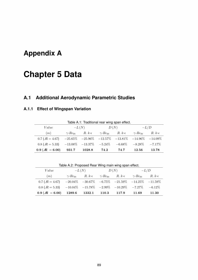
Appendix A

Chapter 5 Data

A.1 Additional Aerodynamic Parametric Studies

A.1.1 Effect of Wingspan Variation

Table A.1: Traditional rear wing span effect.

V alue

(m)

−L (N) D (N) −L/D


0.7 (A = 4.67) −25.65% −25.96% −12.57% −13.81% −14.96% −14.09%

0.8 (A = 5.33) −13.08% −13.37% −5.24% −6.68% −8.28% −7.17%

0.9 (A = 6.00) 931.7 1028.8 74.2 74.7 12.56 13.78

Table A.2: Proposed Rear Wing main wing span effect.

V alue

(m)

−L (N) D (N) −L/D


0.7 (A = 4.67) −20.04% −30.67% −6.75% −21.59% −14.25% −11.59%

0.8 (A = 5.33) −10.04% −15.78% −2.99% −10.29% −7.27% −6.12%

0.9 (A = 6.00) 1289.6 1332.1 110.3 117.9 11.69 11.30

89

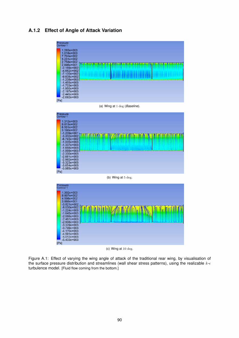
A.1.2 Effect of Angle of Attack Variation

(a) Wing at 1 deg (Baseline).

(b) Wing at 5 deg.

(c) Wing at 10 deg.

Figure A.1: Effect of varying the wing angle of attack of the traditional rear wing, by visualisation of

the surface pressure distribution and streamlines (wall shear stress patterns), using the realizable k-ǫturbulence model. [Fluid flow coming from the bottom.]

90

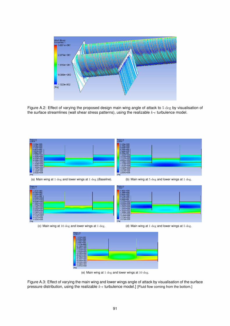
Figure A.2: Effect of varying the proposed design main wing angle of attack to 5 deg by visualisation of

the surface streamlines (wall shear stress patterns), using the realizable k-ǫ turbulence model.

(a) Main wing at 1 deg and lower wings at 1 deg (Baseline). (b) Main wing at 5 deg and lower wings at 1 deg.

(c) Main wing at 10 deg and lower wings at 1 deg. (d) Main wing at 1 deg and lower wings at 5 deg.

(e) Main wing at 1 deg and lower wings at 10 deg.

Figure A.3: Effect of varying the main wing and lower wings angle of attack by visualisation of the surface

pressure distribution, using the realizable k-ǫ turbulence model.] [Fluid flow coming from the bottom.]

91

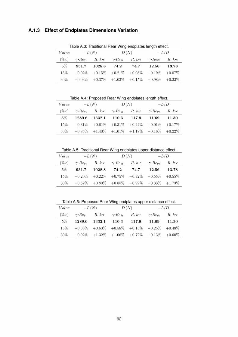
A.1.3 Effect of Endplates Dimensions Variation

Table A.3: Traditional Rear Wing endplates length effect.

V alue

(% c)

−L (N) D (N) −L/D


5% 931.7 1028.8 74.2 74.7 12.56 13.78

15% +0.02% +0.15% +0.21% +0.08% −0.19% +0.07%

30% +0.03% +0.37% +1.03% +0.15% −0.98% +0.22%

Table A.4: Proposed Rear Wing endplates length effect.

V alue

(% c)

−L (N) D (N) −L/D


5% 1289.6 1332.1 110.3 117.9 11.69 11.30

15% +0.31% +0.61% +0.31% +0.44% +0.01% +0.17%

30% +0.85% +1.40% +1.01% +1.18% −0.16% +0.22%

Table A.5: Traditional Rear Wing endplates upper distance effect.

V alue

(% c)

−L (N) D (N) −L/D


5% 931.7 1028.8 74.2 74.7 12.56 13.78

15% +0.20% +0.22% +0.75% −0.32% −0.55% +0.55%

30% +0.52% +0.80% +0.85% −0.92% −0.33% +1.73%

Table A.6: Proposed Rear Wing endplates upper distance effect.

V alue

(% c)

−L (N) D (N) −L/D


5% 1289.6 1332.1 110.3 117.9 11.69 11.30

15% +0.33% +0.63% +0.58% +0.15% −0.25% +0.48%

30% +0.92% +1.32% +1.06% +0.72% −0.13% +0.60%

92

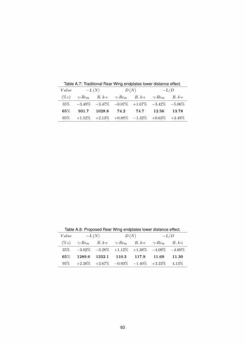
Table A.7: Traditional Rear Wing endplates lower distance effect.

V alue

(% c)

−L (N) D (N) −L/D


35% −3.49% −3.47% −0.07% +1.67% −3.42% −5.06%

65% 931.7 1028.8 74.2 74.7 12.56 13.78

95% +1.52% +2.13% +0.88% −1.32% +0.63% +3.49%

Table A.8: Proposed Rear Wing endplates lower distance effect.

V alue

(% c)

−L (N) D (N) −L/D


35% −3.02% −3.28% +1.12% +1.38% −4.09% −4.60%

65% 1289.6 1332.1 110.3 117.9 11.69 11.30

95% +2.26% +2.67% −0.93% −1.40% +3.22% 4.13%

93

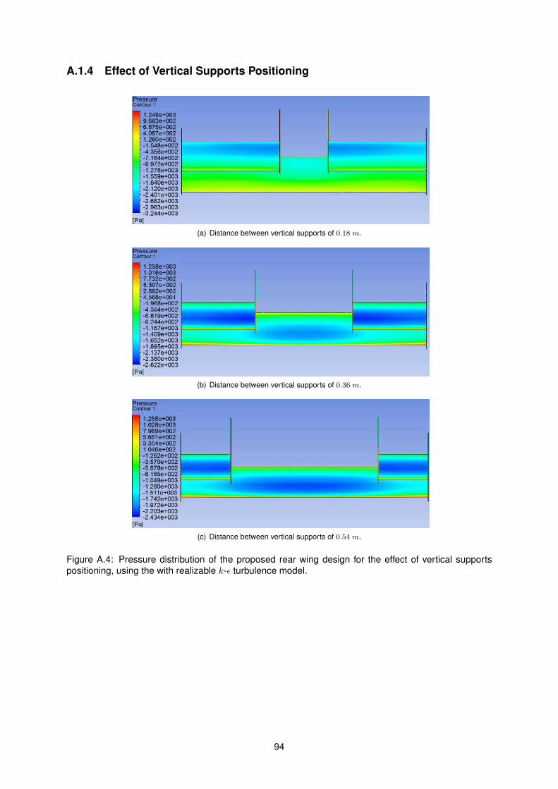
A.1.4 Effect of Vertical Supports Positioning

(a) Distance between vertical supports of 0.18 m.

(b) Distance between vertical supports of 0.36 m.

(c) Distance between vertical supports of 0.54 m.

Figure A.4: Pressure distribution of the proposed rear wing design for the effect of vertical supports

positioning, using the with realizable k-ǫ turbulence model.

94

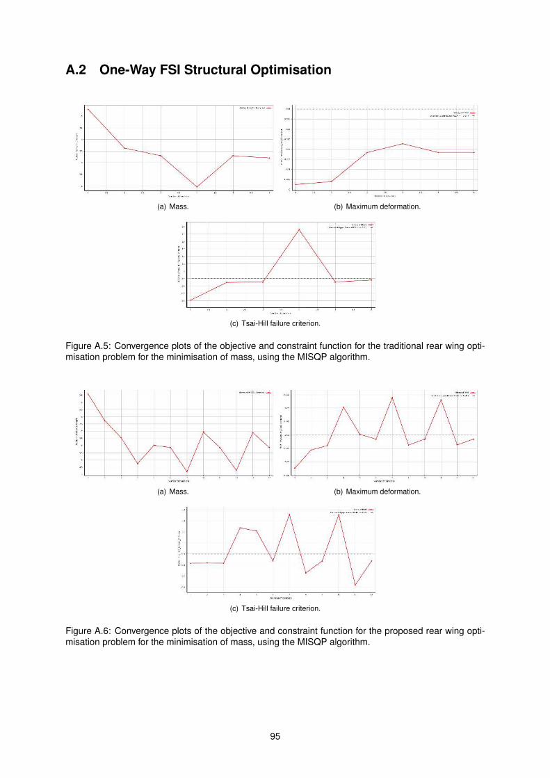
A.2 One-Way FSI Structural Optimisation

(a) Mass. (b) Maximum deformation.

(c) Tsai-Hill failure criterion.

Figure A.5: Convergence plots of the objective and constraint function for the traditional rear wing opti-

misation problem for the minimisation of mass, using the MISQP algorithm.

(a) Mass. (b) Maximum deformation.

(c) Tsai-Hill failure criterion.

Figure A.6: Convergence plots of the objective and constraint function for the proposed rear wing opti-

misation problem for the minimisation of mass, using the MISQP algorithm.

95

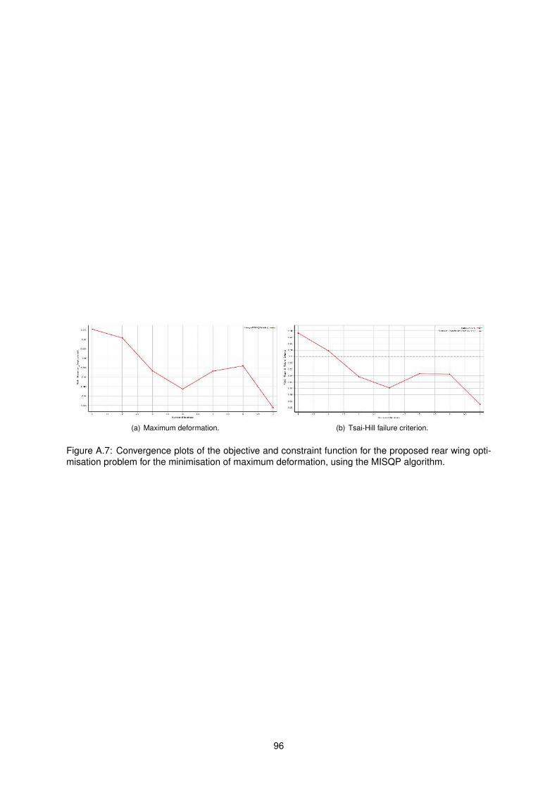
(a) Maximum deformation. (b) Tsai-Hill failure criterion.

Figure A.7: Convergence plots of the objective and constraint function for the proposed rear wing opti-

misation problem for the minimisation of maximum deformation, using the MISQP algorithm.

96

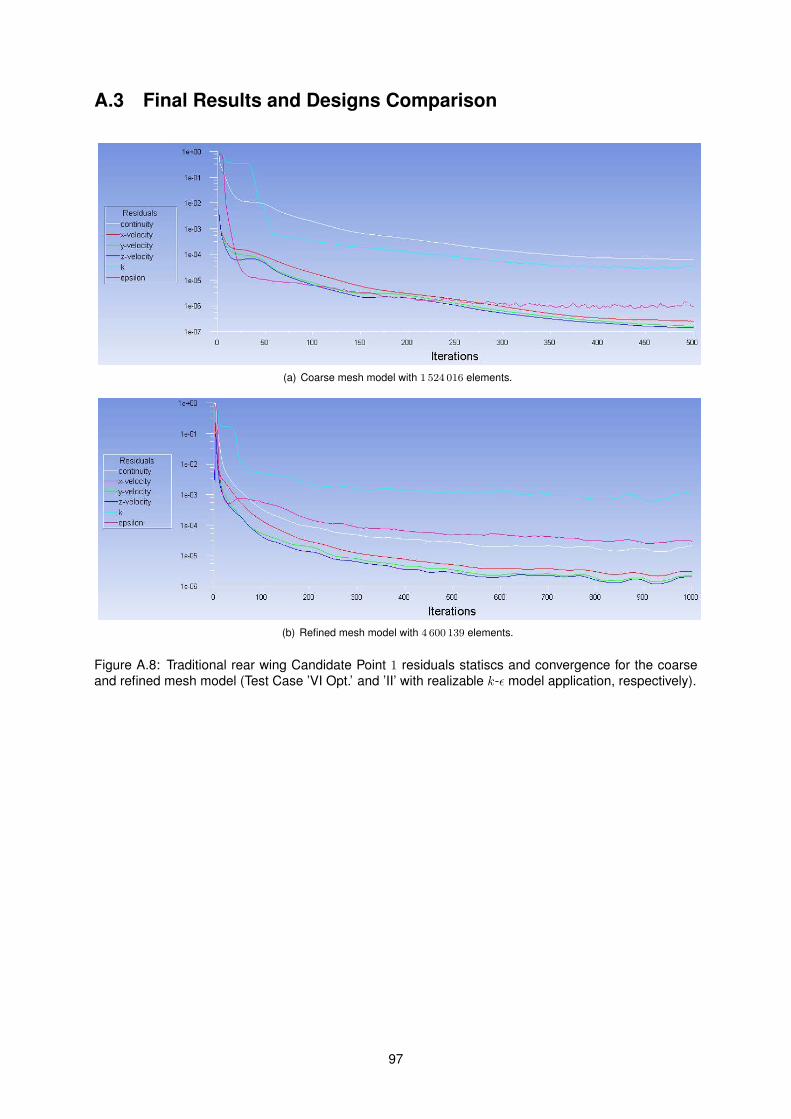
A.3 Final Results and Designs Comparison

(a) Coarse mesh model with 1 524 016 elements.

(b) Refined mesh model with 4 600 139 elements.

Figure A.8: Traditional rear wing Candidate Point 1 residuals statiscs and convergence for the coarse

and refined mesh model (Test Case ’VI Opt.’ and ’II’ with realizable k-ǫ model application, respectively).

97

Appendix B

Material Properties Data Sheets

Notes for derived shear properties according to [67]:

1. Derived properties for balance laminate at 45◦ to fibre direction;

2. Young’s Modulus is derived from the averaged tensile and compressive moduli in 1- (longitudinal)

and 2- (transverse) direction of the ply;

3. Strains are corrected for the average moduli;

4. From tensor rotation algebra it can be seen that shear strains of 45◦ plies are twice the strains

in the ply’s 1- and 2- direction. Limit shear strains are ”rotated” transverse tensile resin failure

strains. Ultimate shear strains are ”rotated” longitudinal compressive fibre failure or transverse

compressive resin failure, whichever is least;

5. Set Safety Factor between limit and ultimate load as required. Default value 1.5.

99

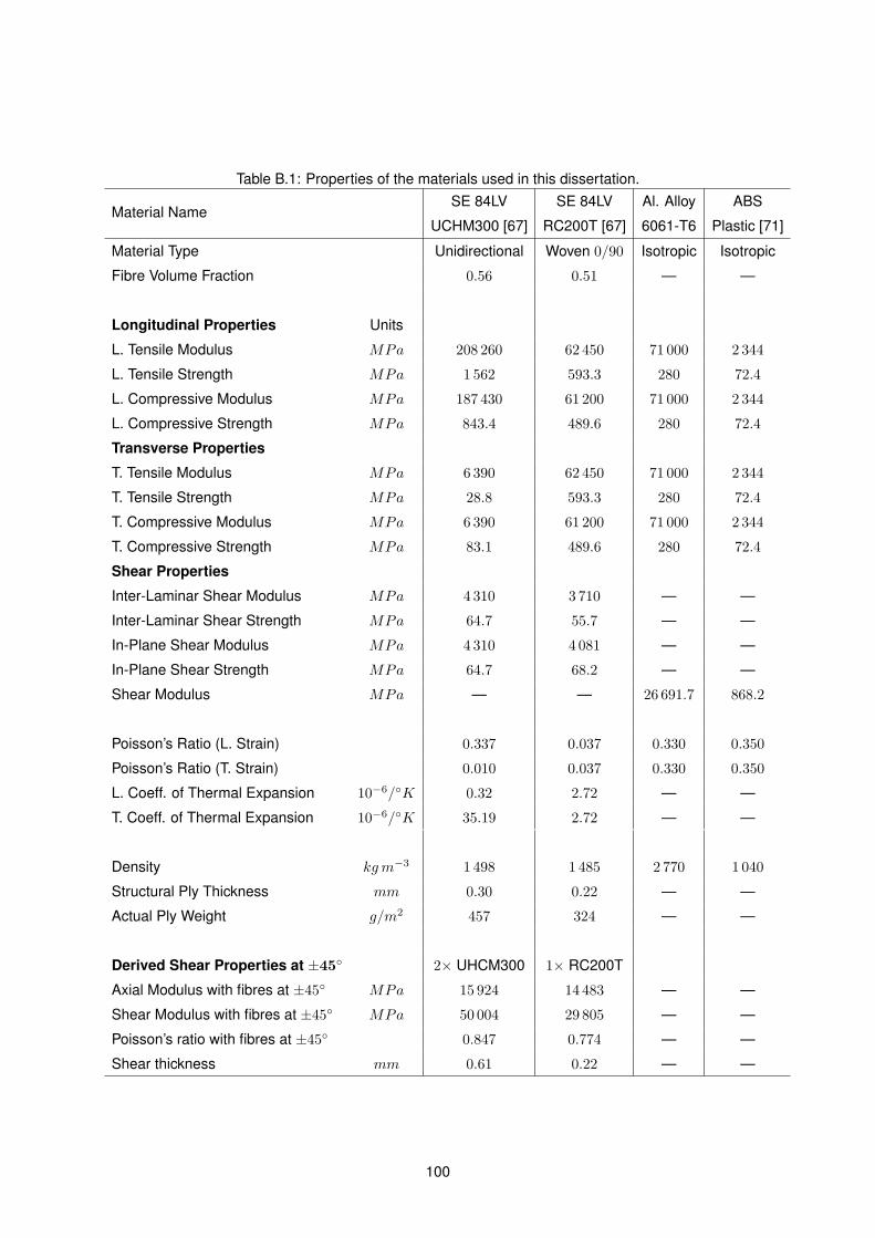
Table B.1: Properties of the materials used in this dissertation.

Material NameSE 84LV

UCHM300 [67]

SE 84LV

RC200T [67]

Al. Alloy

6061-T6

ABS

Plastic [71]

Material Type Unidirectional Woven 0/90 Isotropic Isotropic

Fibre Volume Fraction 0.56 0.51 — —

Longitudinal Properties Units

L. Tensile Modulus MPa 208 260 62 450 71 000 2 344

L. Tensile Strength MPa 1 562 593.3 280 72.4

L. Compressive Modulus MPa 187 430 61 200 71 000 2 344

L. Compressive Strength MPa 843.4 489.6 280 72.4

Transverse Properties

T. Tensile Modulus MPa 6 390 62 450 71 000 2 344

T. Tensile Strength MPa 28.8 593.3 280 72.4

T. Compressive Modulus MPa 6 390 61 200 71 000 2 344

T. Compressive Strength MPa 83.1 489.6 280 72.4

Shear Properties

Inter-Laminar Shear Modulus MPa 4 310 3 710 — —

Inter-Laminar Shear Strength MPa 64.7 55.7 — —

In-Plane Shear Modulus MPa 4 310 4 081 — —

In-Plane Shear Strength MPa 64.7 68.2 — —

Shear Modulus MPa — — 26 691.7 868.2

Poisson’s Ratio (L. Strain) 0.337 0.037 0.330 0.350

Poisson’s Ratio (T. Strain) 0.010 0.037 0.330 0.350

L. Coeff. of Thermal Expansion 10−6/◦K 0.32 2.72 — —

T. Coeff. of Thermal Expansion 10−6/◦K 35.19 2.72 — —

Density kgm−3 1 498 1 485 2 770 1 040

Structural Ply Thickness mm 0.30 0.22 — —

Actual Ply Weight g/m2 457 324 — —

Derived Shear Properties at ±45◦ 2× UHCM300 1× RC200T

Axial Modulus with fibres at ±45◦ MPa 15 924 14 483 — —

Shear Modulus with fibres at ±45◦ MPa 50 004 29 805 — —

Poisson’s ratio with fibres at ±45◦ 0.847 0.774 — —

Shear thickness mm 0.61 0.22 — —

100

Multidisciplinary Design Analysis and Optimisation of … Governing Equations of Solid Structure ......

Documents

Transcript of Multidisciplinary Design Analysis and Optimisation of … Governing Equations of Solid Structure ......