Multichannel and Multicarrier Systems · • Here we focus on AWGN channels (multi-carrier/channel...
32
Multichannel and Multicarrier Systems PD0192F Digital Communications JOÃO VIEIRA
Transcript of Multichannel and Multicarrier Systems · • Here we focus on AWGN channels (multi-carrier/channel...

Multichannel and Multicarrier Systems PD0192F Digital Communications
JOÃO VIEIRA

Outline
• Multichannel digital Communications in AWGN channels;
• Multicarrier communications:
– SC vs MC;
– Capacity of Nonideal linear channels;
– OFDM – modulation and demodulation;
– FFT implementation;
– Spectral characteristics;
– Bit and power allocation;
– Peak-to-Average Ratio

Quick Intro
• In some applications, its desirable to transmit the same signal in
different channels is prefered when using unreliable channels w/
high probability;
• Same information in multiple channels diversity;
• Another form of multichannel comm. is multicarrier transmission,
where a freq. band is subdivided into a number of subchannels (and
information is transmitted in each of the subchannels);
• This chapter covers multichannel and multicarrier signal
transmission;
• Here we focus on AWGN channels (multi-carrier/channel in fading
channels is addressed in Chapter 13).

11.1- Multichannel Digital
communications in AWGN channels
Channels are fixed and only differ in magnitude and phase;
Waveforms have equal energy and are equally likely;
N. channels N. waveforms

11.1- Multichannel Digital
communications in AWGN channels
Decision
variables
For coherent detection:

11.1- Multichannel Digital
communications in AWGN channels
For non-coherent detection:
For binary signaling and assuming that
are the transmitted waveforms. An error is commited if:
or
Square law
Detection
(easier to analyse)
No attempt is made to estimate the channel parameters;
Detector decision is based on the sum of envelopes or sum of
squared envelopes (square law detection) of the MF outputs;

11.1- Multichannel Digital
communications in AWGN channels
For non-coherent detection:
For binary signaling and assuming that
are the transmitted waveforms. An error is commited if:
or
For non-coherent detection:

11.1- Multichannel Digital
communications in AWGN channels
For binary signaling and assuming that
are the transmitted waveforms. An error is commited if:
or
For coherent detection:
For coherent detection:

11.1-1 Binary Signals
The error probability for binary multichannel signalling in
AWGN is derived in Appendix B.
– Antipodal signals + perfect estimation of
– Rx combines energy of L channels such that no loss/gain in performance
when dividing Tx signal energy in channels;
• This holds if . If the estimates are not perfect, a loss in performance
occurs (Appendix C).
SNR per bit
If , ∀ n
Total Tx signal energy for the L signals.

11.1-1 Binary Signals
Perfect CSI is an extreme case. On the other extreme DPSK;
“In differentially encoded PSK, the information sequence determines the relative phase, or
phase transition, between adjacent symbol intervals”
“Key assumption … phase offset φ remains the same over adjacent signaling periods”

11.1-1 Binary Signals
Perfect CSI is an extreme case. On the other extreme DPSK;
If , for the same SNR/bit the multichannel performance
poorer than single-channel system splitting energy performance loss;
, ∀ n
“In differentially encoded PSK, the information sequence determines the relative phase, or
phase transition, between adjacent symbol intervals”

11.1-1 Binary Signals

11.1-1 Binary Signals
• A loss in performance also occurs in square law detection of orthogonal signals
transmitted in L channels; For binary orthogonal signalling Pe is identical to DPSK
but 3dB poorer ,i.e., 𝛾𝑏 is replaced by 𝛾𝑏
2 and the peformance loss due to
non-coherent combination of the L received signals is identical.

11.2 Multicarrier Communications
• (One) Motivation: reduce ISI and performance degradation
compared to SC systems.

11.2 Single-Carrier Vs Multicarrier
modulation
• If and are constant, the channel is ideal or
nondistorting;
• If we use single carrier on nonideal linear channels ISI since
the time dispersion >> symbol rate equalizer is necessary;
• Alternatively, we can divide the BW into almost ideal channels:
Let be the frequency response of a nonideal, band-limited channel
~ constant within
each sub-band
Constrain

11.2-2 – Capacity of a Nonideal Linear
Filter Channel
• Recall : (for ideal, band-limited AWGN)
• In multicarrier system
• When
• Under the previous constaint, the choice of P(f) that maximizes C
is choosen by maximizing:

11.2-2 – Capacity of a Nonideal Linear
Filter Channel
• The optimum distribution of Tx power:
• Basic interpretation: High power @ High SNR

11.2-3 – Orthogonal Frequency
Division Multiplexing (OFDM)
• Dividing channel into small sub-bands
can yield TX rates close to channel capacity
• Independently coded and modulated;
• Flat for each sub band -> no ISI.
• For each subchannel:
• If Δ𝑓 =1
𝑇
• OFDM is a special case of multichnnel mod. where subcarrier
acting in subchannel are mutually orthogonal.

11.2-4 – Modulation and demodulation
in an OFDM system
• With N large 𝑇 ≫ 𝜏𝑚𝑎𝑥 hence, fixed
• If QAM in each subcarrier, the signal @ k^th subcarrier can
be expressed as:
QAM signal point
In k^th subcarrier
symbol time in a SC system

11.2-4 – Modulation and demodulation
in an OFDM system
• The received signal in the k^th subchannel is
• We assume 𝐶𝑘 and ϕ𝑘 known @ Rx;

11.2-4 – Modulation and demodulation
in an OFDM system
• Demodulation on the kth subcarrier cross correlating 𝑟𝑘(𝑡) with the 2
basis, given that we know {ϕ𝑘}:
• and sampling the output of the cross-correlators at t = T, we obtain:
• Expressed as complex number:
• Scaling the received sybol by channel gain
Passed to detector

11.2-4 – Modulation and demodulation
in an OFDM system
• Demodulation on the kth subcarrier cross correlating 𝑟𝑘(𝑡) with the 2
basis, given that we know {ϕ𝑘}:
• and sampling the output of the cross-correlators at t = T, we obtain:
From this description, 2 correlators (or 2 matched filters) per subcarrier to
demodulate the Rx signal. In an OFDM system 2N correlators;
This bank of 2N filters is equiv. to computation of DFT and its
inverse. Hence, FFT is an efficient tool to implement this system.

11.2-5 – An FFT Algorithm
Implementation of an OFDM system
Computation of IDFT of the data {X_k}, can be viewed as multiplication
of each data point X_k by a corresponding vector:

11.2-5 – An FFT Algorithm
Implementation of an OFDM system

11.2-5 – An FFT Algorithm
Implementation of an OFDM system
• Avoid ISI append cyclic prefix. (Re-indexing from –v to N-1);
• Conv. of with produces
• We are interested in thus the first v
samples can be discarded;
• Note: OFDM is not optimal;
11.2-5 – An FFT Algorithm
Implementation of an OFDM system
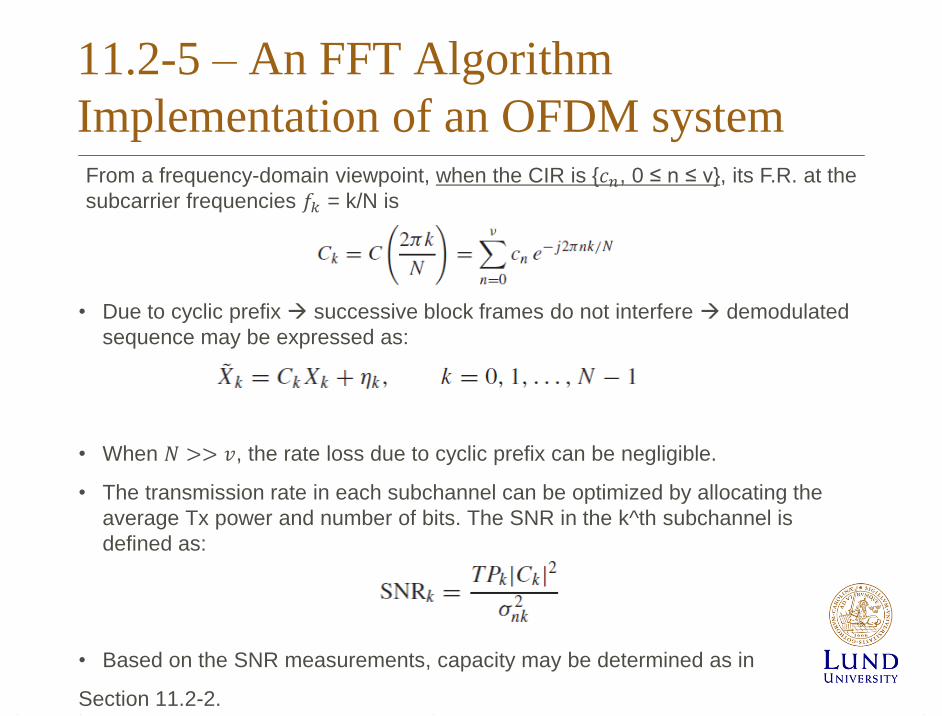
• Due to cyclic prefix successive block frames do not interfere demodulated
sequence may be expressed as:
• When 𝑁 >> 𝑣, the rate loss due to cyclic prefix can be negligible.
• The transmission rate in each subchannel can be optimized by allocating the
average Tx power and number of bits. The SNR in the k^th subchannel is
defined as:
• Based on the SNR measurements, capacity may be determined as in
Section 11.2-2.
From a frequency-domain viewpoint, when the CIR is {𝑐𝑛, 0 ≤ n ≤ ν}, its F.R. at the
subcarrier frequencies 𝑓𝑘 = k/N is

11.2-6 – Spectral Characteristics of
Multicarrier systems
• OFDM subcarrier signals in are mutually orthogonal in time, they overlap in
frequency. This can be seen by computing the F.T. of the signal
• Spectral overlap of the main lobes but
signals are still orthogonal when transmitted
synchronously;
Sidenote: Doopler destroys orthogonality
among subcarriers;

11.2-7 – Bit and Power allocation in
Multicarrier Modulation
• … to optimize performance of MC system operatnig in linear-time AWGN channels;
• We assume Ñ subcarriers using QAM with 𝑀𝑖 = 2𝑏𝑖, and 𝑏𝑖 bits are transmitted in
the i^th subcarrier during T seconds.
• We assume complex constant 𝐶(𝑓𝑖) and flat noise PSD (across subchannels);
• Objective maximize Rb for a given Pe with is the same across the Ñ
subchannels (subject to a power constaint);
Error prob. For QAM
@ low error rates
total
bitrate

11.2-8 – Peak-to-Average Ratio in
Multicarrier Modulation
• A major problem in MC modulation is the peak-to-average-power-ratio (PAPR);
occurs where many subchannels add constructively in phase;
Diff notation
Problem: the whole transmitter chain
(from baseband to antenna) needs to
have a linear/ high dynamic range.

11.2-8 – Peak-to-Average Ratio in
Multicarrier Modulation
• Clipping of the signal voltage in a D/A can happen, or it can saturate the power
amplifier in this, cause intermodulation distortion;
PAPR reducing methods:
• Tone-reservation: add a peak-annihilating signal c(n) to the transmit s(n). c(n)
is chosen such that it has counter-peaks peaks of s(n)+c(n) are lower than the
ones of s(n) .
Subcarriers need to be sacrificed;
• The desired “good” peak-annihilating property can be formulated as minimisation
problem:
average power per
signal sample

11.2-8 – Peak-to-Average Ratio in
Multicarrier Modulation
PAPR reducing methods:
• Tone-reservation;
• Tone-injection: same idea as tone-reservation (adding a peak-annihilating
signal); However, no tones are reserved: peak-annihilating signals are added on data-
carrying tones.
• Based on module principle;
• Rx has to know that the Tx may chose
to send points from the extended constellation;
• Selecting symbols from the extended
constellation increases the average Tx power
• (Connected with Tomlinson-Harashima
precoding in Section 9.5-4 ?;)