Multiagent Learning - Foundations and Recent Trendslarg/ijcai17_tutorial/multiagent... ·...
186
Multiagent Learning Foundations and Recent Trends Stefano Albrecht and Peter Stone Tutorial at IJCAI 2017 conference: http://www.cs.utexas.edu/~larg/ijcai17_tutorial
Transcript of Multiagent Learning - Foundations and Recent Trendslarg/ijcai17_tutorial/multiagent... ·...

Multiagent LearningFoundations and Recent Trends
Stefano Albrecht and Peter Stone
Tutorial at IJCAI 2017 conference:http://www.cs.utexas.edu/~larg/ijcai17_tutorial

Overview
Introduction
Multiagent Models & Assumptions
Learning Goals
Learning Algorithms
Recent Trends
S. Albrecht, P. Stone 1

Multiagent Systems
• Multiple agents interact incommon environment
• Each agent with ownsensors, effectors, goals, ...
• Agents have to coordinateactions to achieve goals
Environment
effectors
sensors
knowledge
Domain
Agent
Goals
Goals
Agent
Actions
Actions
Domain
knowledge
S. Albrecht, P. Stone 2

Multiagent Systems
Environment defined by:• state space• available actions• effects of actions on states• what agents can observe
Agents defined by:• domain knowledge• goal specification• policies for selecting actions
Environment
effectors
sensors
knowledge
Domain
Agent
Goals
Goals
Agent
Actions
Actions
Domain
knowledge
Many problems can be modelled as multiagent systems!
S. Albrecht, P. Stone 3

Multiagent Systems – Applications
Chess Poker Starcraft
Robot soccer Home assistance Autonomous cars
S. Albrecht, P. Stone 4

Multiagent Systems – Applications
Chess Poker Starcraft
Robot soccer Home assistance Autonomous cars
S. Albrecht, P. Stone 4

Multiagent Systems – Applications
Negotiation Wireless networks Smart grid
User interfaces Multi-robot rescue
S. Albrecht, P. Stone 5

Multiagent Systems – Applications
Negotiation Wireless networks Smart grid
User interfaces Multi-robot rescue
S. Albrecht, P. Stone 5

Multiagent Learning
Multiagent learning• Learning is process of improving performance via experience• Can agents learn to coordinate actions with other agents?• What to learn?
⇒ How to select own actions⇒ How other agents select actions⇒ Other agents’ goals, plans, beliefs, ...
S. Albrecht, P. Stone 6

Multiagent Learning
Multiagent learning• Learning is process of improving performance via experience• Can agents learn to coordinate actions with other agents?• What to learn?⇒ How to select own actions
⇒ How other agents select actions⇒ Other agents’ goals, plans, beliefs, ...
S. Albrecht, P. Stone 6

Multiagent Learning
Multiagent learning• Learning is process of improving performance via experience• Can agents learn to coordinate actions with other agents?• What to learn?⇒ How to select own actions⇒ How other agents select actions
⇒ Other agents’ goals, plans, beliefs, ...
S. Albrecht, P. Stone 6

Multiagent Learning
Multiagent learning• Learning is process of improving performance via experience• Can agents learn to coordinate actions with other agents?• What to learn?⇒ How to select own actions⇒ How other agents select actions⇒ Other agents’ goals, plans, beliefs, ...
S. Albrecht, P. Stone 6

Multiagent Learning
Why learning?• Domain too complex to solve by hand or with multiagent planninge.g. computing equilibrium solutions in games
• Elements of domain unknowne.g. observation probabilities, behaviours of other agents, ...⇒ Multiagent planning requires complete model
• Other agents may learn too⇒ Have to adapt continually!“Moving target problem” central issue in multiagent learning
S. Albrecht, P. Stone 7

Research in Multiagent Learning
Multiagent learning studied in different communities
• AI, game theory, robotics, psychology, ...
• Some conferences & journals: AAMAS, AAAI, IJCAI, NIPS, UAI, ICML,ICRA, IROS, RSS, PRIMA, JAAMAS, AIJ, JAIR, MLJ, JMLR, ...⇒ Very large + growing body of work!
• Many algorithms proposed to address different assumptions(constraints), learning goals, performance criteria, ...
S. Albrecht, P. Stone 8

Tutorial
This tutorial:• Introduction to basics of multiagent learning:
• Interaction models & assumptions• Learning goals• Selection of learning algorithms
• Plus some recent trends
Further reading:• AIJ Special Issue “Foundations of Multi-Agent Learning”Rakesh Vohra, Michael Wellman (eds.), 2007
• Surveys: Tuyls and Weiss (2012); Busoniu et al. (2008); Panait andLuke (2005); Shoham et al. (2003); Alonso et al. (2001); Stone andVeloso (2000); Sen and Weiss (1999)
• Our own upcoming survey on agents modelling other agents!
S. Albrecht, P. Stone 9
Overview
Introduction
Multiagent Models & Assumptions
Learning Goals
Learning Algorithms
Recent Trends
S. Albrecht, P. Stone 10

Overview
Introduction
Multiagent Models & Assumptions
Learning Goals
Learning Algorithms
Recent Trends
S. Albrecht, P. Stone 11

Multiagent Models & Assumptions
Standard multiagent models:
• Normal-form game• Repeated game• Stochastic game
Assumptions and other models
S. Albrecht, P. Stone 12

Normal-Form Game
Normal-form game consists of:• Finite set of agents N = {1, ...,n}• For each agent i ∈ N:
• Finite set of actions Ai• Utility function ui : A→ R, where A = A1 × ...× An
Each agent i selects policy πi : Ai → [0, 1], takes action ai ∈ Ai withprobability πi(ai), and receives utility ui(a1, ...,an)
Given policy profile (π1, ..., πn), expected utility to i is
Ui(π1, ..., πn) =∑a∈ A
π1(a1) ∗ ... ∗ πn(an) ∗ ui(a)
⇒ Agents want to maximise their expected utilities
S. Albrecht, P. Stone 13

Normal-Form Game: Prisoner’s Dilemma
Example: Prisoner’s Dilemma• Two prisoners questioned in isolated cells• Each prisoner can Cooperate or Defect• Utilities (row = agent 1, column = agent 2):
C DC -1,-1 -5,0D 0,-5 -3,-3
S. Albrecht, P. Stone 14

Normal-Form Game: Chicken
Example: Chicken• Two opposite drivers on same lane• Each driver can Stay on lane or Leave lane• Utilities:
S LS 0,0 7,2L 2,7 6,6
S. Albrecht, P. Stone 15

Normal-Form Game: Rock-Paper-Scissors
Example: Rock-Paper-Scissors• Two players, three actions• Rock beats Scissors beats Paper beats Rock• Utilities:
R P SR 0,0 -1,1 1,-1P 1,-1 0,0 -1,1S -1,1 1,-1 0,0
S. Albrecht, P. Stone 16

Repeated Game
Learning requires experience
• Normal-form game is single interaction⇒ No experience!
• Experience comes from repeated interactions
Repeated game:• Repeat same normal-form game: at each time t, each agent ichooses action ati and gets utility ui(at1, ...,atn)
• Policy πi : H× Ai → [0, 1] assigns action probabilities based onhistory of interaction
H = ∪t∈N0Ht, Ht ={Ht = (a0,a1, ...,at−1) | aτ ∈ A
}
S. Albrecht, P. Stone 17

Repeated Game
What is expected utility to i for policy profile (π1, ..., πn)?
• Repeating game t ∈ N times:
Ui(π1, ..., πn) =∑Ht∈Ht
P(Ht|π1, ..., πn)t−1∑τ=0
ui(aτ )
P(Ht|π1, ..., πn) =t−1∏τ=0
∏j∈N
πj(Hτ ,aτj )
S. Albrecht, P. Stone 18

Repeated Game
What is expected utility to i for policy profile (π1, ..., πn)?
• Repeating game∞ times:
Ui(π1, ..., πn) = limt→∞
∑Ht
P(Ht|π1, ..., πn)∑τ
γτui(aτ )
Discount factor 0 ≤ γ < 1 makes expectation finite
Interpretation: low γ is “myopic”, high γ is “farsighted”(Or: probability that game will end at each time is 1− γ)
Can also define expected utility as limit average
S. Albrecht, P. Stone 19

Repeated Game: Prisoner’s Dilemma
Example: Repeated Prisoner’s Dilemma
C DC -1,-1 -5,0D 0,-5 -3,-3
Example policies:
• At time t, choose C with probability (t+ 1)−1
• Grim: chose C until opponent’s first D, then choose D forever• Tit-for-Tat: begin C, then repeat opponent’s last action
S. Albrecht, P. Stone 20

Repeated Game: Rock-Paper-Scissors
Example: Repeated Rock-Paper-Scissors
R P SR 0,0 -1,1 1,-1P 1,-1 0,0 -1,1S -1,1 1,-1 0,0
Example policy:• Compute empirical frequency of opponent actions over past 5moves
P(aj) =15
t−1∑τ=t−5
[aτj = aj]1
and take best-response action maxai∑
aj P(aj)ui(ai,aj)
S. Albrecht, P. Stone 21

Stochastic Game
Agents interact in common environment
• Environment has states, actions have effect on state• Agents choose actions based on state-action history
Example: Pursuit (e.g. Barrett et al., 2011)• Predator agents must capture prey• State: agent positions• Actions: move to neighbouring cell
S. Albrecht, P. Stone 22

Stochastic Game
Stochastic game consists of:• Finite set of agents N = {1, ...,n}• Finite set of states S• For each agent i ∈ N:
• Finite set of actions Ai• Utility function ui : S× A→ R, where A = A1 × ...× An
• State transition function T : S× A× S→ [0, 1]
Generalises Markov decision process (MDP) to multiple agents
S. Albrecht, P. Stone 23

Stochastic Game
Game starts in initial state s0 ∈ S
At each time t:
• Each agent i...
• observes current state st and past joint action at−1 (if t > 0)• chooses action ati ∈ Ai with probability πi(Ht,ati) whereHt = (s0,a0, s1,a1, ..., st−1) is state-action history
• receives utility ui(at1, ...,atn)• Game transitions into next state st+1 ∈ S with probabilityT(st,at, st+1)
Process repeated finite or infinite number of times, or until terminalstate is reached (e.g. prey captured).
S. Albrecht, P. Stone 24

Stochastic Game
Game starts in initial state s0 ∈ S
At each time t:
• Each agent i...• observes current state st and past joint action at−1 (if t > 0)
• chooses action ati ∈ Ai with probability πi(Ht,ati) whereHt = (s0,a0, s1,a1, ..., st−1) is state-action history
• receives utility ui(at1, ...,atn)• Game transitions into next state st+1 ∈ S with probabilityT(st,at, st+1)
Process repeated finite or infinite number of times, or until terminalstate is reached (e.g. prey captured).
S. Albrecht, P. Stone 24

Stochastic Game
Game starts in initial state s0 ∈ S
At each time t:
• Each agent i...• observes current state st and past joint action at−1 (if t > 0)• chooses action ati ∈ Ai with probability πi(Ht,ati) whereHt = (s0,a0, s1,a1, ..., st−1) is state-action history
• receives utility ui(at1, ...,atn)
• Game transitions into next state st+1 ∈ S with probabilityT(st,at, st+1)
Process repeated finite or infinite number of times, or until terminalstate is reached (e.g. prey captured).
S. Albrecht, P. Stone 24

Stochastic Game
Game starts in initial state s0 ∈ S
At each time t:
• Each agent i...• observes current state st and past joint action at−1 (if t > 0)• chooses action ati ∈ Ai with probability πi(Ht,ati) whereHt = (s0,a0, s1,a1, ..., st−1) is state-action history
• receives utility ui(at1, ...,atn)• Game transitions into next state st+1 ∈ S with probabilityT(st,at, st+1)
Process repeated finite or infinite number of times, or until terminalstate is reached (e.g. prey captured).
S. Albrecht, P. Stone 24

Stochastic Game
Game starts in initial state s0 ∈ S
At each time t:
• Each agent i...• observes current state st and past joint action at−1 (if t > 0)• chooses action ati ∈ Ai with probability πi(Ht,ati) whereHt = (s0,a0, s1,a1, ..., st−1) is state-action history
• receives utility ui(at1, ...,atn)• Game transitions into next state st+1 ∈ S with probabilityT(st,at, st+1)
Process repeated finite or infinite number of times, or until terminalstate is reached (e.g. prey captured).
S. Albrecht, P. Stone 24

Stochastic Game: Level-Based Foraging
Example: Level-Based Foraging (Albrecht and Ramamoorthy, 2013)• Agents (circles) must collect all items (squares)• State: agent positions, item positions, which items collected• Actions: move to neighbouring cell, try to collect item
S. Albrecht, P. Stone 25

Stochastic Game: Soccer Keepaway
Example: Soccer Keepaway (Stone et al., 2005)• “Keeper” agents must keep ball away from “Taker” agents• State: player positions & orientations, ball position, ...• Actions: go to ball, pass ball to player, ...
S. Albrecht, P. Stone 26

Stochastic Game: Soccer Keepaway
Video: 4 vs 3 Keepaway
Source: http://www.cs.utexas.edu/~AustinVilla/sim/keepaway
S. Albrecht, P. Stone 27

Assumptions
Models and algorithms make assumptions, e.g.
• What do agents know about the game?• What can agents observe during a game?
Usual assumptions:
• Game elements known (state/action space, utility function, ...)• Game states & chosen actions are commonly observed⇒ “full observability” or “perfect information”
Many learning algorithms designed for repeated/stochastic gamewith full observability
• But assumptions may vary and other models exist!
S. Albrecht, P. Stone 28

Other Models
Other assumptions & models:
• Assumption: elements of game unknown
• Bayesian game, stochastic Bayesian gameAAAI’16 tutorial “Type-based Methods for Interaction inMultiagent Systems”http://thinc.cs.uga.edu/tutorials/aaai-16.html
• Assumption: partial observability of states and actions
• Extensive-form game with imperfect information• Partially observable stochastic game (POSG)• Multiagent POMDPs: Dec-POMDP, I-POMDP, ...
S. Albrecht, P. Stone 29

Overview
Introduction
Multiagent Models & Assumptions
Learning Goals
Learning Algorithms
Recent Trends
S. Albrecht, P. Stone 30

Learning Goals
Learning is to improve performance via experience
• But what is goal (end-result) of learning process?• How to measure success of learning?
Many learning goals proposed:
• Minimax/Nash/correlated equilibrium• Pareto-optimality• Social welfare & fairness• No-regret• Targeted optimality & safety
... plus combinations & approximations
S. Albrecht, P. Stone 31

Maximin/Minimax
Two-player zero-sum game: ui = −uj• e.g. Rock-Paper-Scissors, Chess
Policy profile (πi, πj) is maximin/minimax profile if
Ui(πi, πj) = maxπ′i
minπ′j
Ui(π′i , π
′j ) = min
π′j
maxπ′j
Ui(π′i , π
′j ) = −Uj(πi, πj)
Utility that can be guaranteed against worst-case opponent
• Every two-player zero-sum normal-form game has minimaxprofile (von Neumann and Morgenstern, 1944)
• Every finite or infinite+discounted zero-sum stochastic game hasminimax profile (Shapley, 1953)
S. Albrecht, P. Stone 32

Nash Equilibrium
Policy profile π = (π1, ..., πn) is Nash equilibrium (NE) if
∀i ∀π′i : Ui(π′
i , π−i) ≤ Ui(π)
No agent can improve utility by unilaterally deviating from profile(every agent plays best-response to other agents)
Every finite normal-form game has at least one NE (Nash, 1950)(also stochastic games, e.g. Fink (1964))
• Standard solution in game theory• In two-player zero-sum game, minimax is same as NE
S. Albrecht, P. Stone 33

Nash Equilibrium – Example
Example: Prisoner’s Dilemma• Only NE in normal-form game is (D,D)• Normal-form NE are also NE in infiniterepeated game
• Infinite repeated game has manymore NE⇒ Folk theorem
Example: Rock-Paper-Scissors• Only NE in normal-form game isπi = πj = ( 13 ,
13 ,
13 )
C DC -1,-1 -5,0D 0,-5 -3,-3
R P SR 0,0 -1,1 1,-1P 1,-1 0,0 -1,1S -1,1 1,-1 0,0
S. Albrecht, P. Stone 34
Correlated Equilibrium
Each agent i observes signal xi with joint distribution ξ(x1, ..., xn)
• E.g. xi is action recommendation to agent i
(π1, ..., πn) is correlated equilibrium (CE) (Aumann, 1974) if no agentcan individually improve its expected utility by deviating fromrecommended actions
• NE is subset of CE→ no correlation• CE easier to compute than NE→ linear program
S. Albrecht, P. Stone 35

Correlated Equilibrium – Example
Example: Chicken
Correlated equilibrium:• ξ(L, L) = ξ(S, L) = ξ(L, S) = 1
3
• ξ(S, S) = 0
Expected utility to both:7 ∗ 1
3 + 2 ∗ 13 + 6 ∗ 1
3 = 5
Nash equilibrium utilities:• πi(S) = 1, πj(S) = 0 → (7, 2)• πi(S) = 0, πj(S) = 1 → (2, 7)• πi(S) = 1
3 , πj(S) =13 → ≈ 4.66
S LS 0,0 7,2L 2,7 6,6
S. Albrecht, P. Stone 36

The Equilibrium Legacy
The “Equilibrium Legacy” in multiagent learning:
• Quickly adopted equilibrium as standard goal of learning• But equilibrium (e.g. NE) has many limitations...
1. Non-uniquenessOften multiple NE exist, how should agents choose same one?
2. IncompletenessNE does not specify behaviours for off-equilibrium paths
3. Sup-optimalityNE not generally same as utility maximisation
4. RationalityNE assumes all agents are rational (= perfect utility maximisers)
S. Albrecht, P. Stone 37

Pareto Optimum
Policy profile π = (π1, ..., πn) is Pareto-optimal if there is no otherprofile π′ such that
∀i : Ui(π′) ≥ Ui(π) and ∃i : Ui(π′) > Ui(π)
Can’t improve one agent without making other agent worse off
0 1 2 3 4 50
1
2
3
4
5
Payoff to player 1
Pa
yo
ff to
pla
ye
r 2
1, 1 4, 1
1, 4 3, 3
Pareto-front is set of allPareto-optimal utilities(red line)
S. Albrecht, P. Stone 38

Pareto Optimum
Policy profile π = (π1, ..., πn) is Pareto-optimal if there is no otherprofile π′ such that
∀i : Ui(π′) ≥ Ui(π) and ∃i : Ui(π′) > Ui(π)
Can’t improve one agent without making other agent worse off
0 1 2 3 4 50
1
2
3
4
5
Payoff to player 1
Pa
yo
ff t
o p
laye
r 2
1, 1 4, 1
1, 4 3, 3
Pareto-front is set of allPareto-optimal utilities(red line)
S. Albrecht, P. Stone 38

Social Welfare & Fairness
Pareto-optimality says nothing about social welfare and fairness
Welfare and fairness of profile π = (π1, ..., πn) often defined as
Welfare(π) =∑i
Ui(π) Fairness(π) =∏i
Ui(π)
π welfare/fairness-optimal if maximum Welfare(π)/Fairness(π)
Any welfare/fairness-optimal π is also Pareto-optimal! (Why?)
S. Albrecht, P. Stone 39

No-Regret
Given history Ht = (a0,a1, ...,at−1), agent i’s regret for not havingtaken action ai is
Ri(ai|Ht) =t−1∑τ=0
ui(ai,aτ−i)− ui(aτi ,aτ−i)
Policy πi achieves no-regret if
∀ai : limt→∞
1t Ri(ai|H
t) ≤ 0
(Other variants exist)
S. Albrecht, P. Stone 40

No-Regret
Given history Ht = (a0,a1, ...,at−1), agent i’s regret for not havingtaken action ai is
Ri(ai|Ht) =t−1∑τ=0
ui(ai,aτ−i)− ui(aτi ,aτ−i)
Policy πi achieves no-regret if
∀ai : limt→∞
1t Ri(ai|H
t) ≤ 0
(Other variants exist)
S. Albrecht, P. Stone 40
No-Regret
Like Nash equilibrium, no-regret widely used in multiagent learning
But, like NE, definition of regret has conceptual issues
• Regret definition assumes other agents don’t change actions
Ri(ai|Ht) =t−1∑τ=0
ui(ai,aτ−i)− ui(aτi ,aτ−i)
⇒ But: entire history may change if different actions taken!
• Thus, minimising regret not generally same as maximising utility(e.g. Crandall, 2014)
S. Albrecht, P. Stone 41

Targeted Optimality & Safety
Many algorithms designed to achieve some version of targetedoptimality and safety:
• If other agent’s policy πj in certain class, agent i’s learning shouldconverge to best-response
Ui(πi, πj) ≈ maxπ′i
Ui(π′i , πj)
• If not in class, learning should at least achieve safety (maximin)utility
Ui(πi, πj) ≈ maxπ′i
minπ′j
Ui(π′i , π
′j )
Policy classes: non-learning, memory-bounded, finite automata, ...
S. Albrecht, P. Stone 42

Overview
Introduction
Multiagent Models & Assumptions
Learning Goals
Learning Algorithms
Recent Trends
S. Albrecht, P. Stone 43

Learning Algorithms – The Internal View
How does learning take place in policy πi?
The internal view:• πi continually modifies internal policy πti based on Ht
• πti has own representation and input format Ht
πi
Ht
atiModify πt−1i → πti
Extract Ht → HtπtiHt
S. Albrecht, P. Stone 44

Learning Algorithms – The Internal View
Internal policy πti :
• Representation: Q-learning, MCTS planner, neural network, ...• Parameters: Q-table, opponent model, connection weights, ...• Input format: most recent state/action, abstract feature vector, ...
πi
Ht
atiModify πt−1i → πti
Extract Ht → HtπtiHt
S. Albrecht, P. Stone 45

Fictitious Play
Simple example: Fictitious Play (FP) (Brown, 1951)
At each time t:
1. Compute opponent’s action frequencies:
P(aj) =1
t+ 1
t∑τ=0
[aτj = aj]1
2. Compute best-response action:
ati ∈ argmaxai
∑aj
P(aj)ui(ai,aj)
Self-play: all agents use fictitious play• If policies converge, policy profile is Nash equilibrium
S. Albrecht, P. Stone 46

Learning Algorithms
Many multiagent learning algorithms exist, e.g.• Minimax-Q (Littman, 1994)• JAL (Claus and Boutilier, 1998)• Regret Matching (Hart and Mas-Colell, 2001, 2000)• FFQ (Littman, 2001)• WoLF-PHC (Bowling and Veloso, 2002)• Nash-Q (Hu and Wellman, 2003)• CE-Q (Greenwald and Hall, 2003)• OAL (Wang and Sandholm, 2003)• ReDVaLeR (Banerjee and Peng, 2004)• GIGA-WoLF (Bowling, 2005)• CJAL (Banerjee and Sen, 2007)• AWESOME (Conitzer and Sandholm, 2007)• CMLeS (Chakraborty and Stone, 2014)• HBA (Albrecht, Crandall, and Ramamoorthy, 2016)
S. Albrecht, P. Stone 47

(Conditional) Joint Action Learning
Joint Action Learning (JAL) (Claus and Boutilier, 1998) andConditional Joint Action Learning (CJAL) (Banerjee and Sen, 2007)learn Q-values for joint actions a ∈ A:
Qt+1(at) = (1− α)Qt(at) + αuti
• uti is utility received after joint action at
• α ∈ [0, 1] is learning rate
Use opponent model to compute expected utilities of actions:
JAL: E(ai) =∑aj
P(aj)Qt+1(ai,aj)
CJAL: E(ai) =∑aj
P(aj|ai)Qt+1(ai,aj)
S. Albrecht, P. Stone 48

(Conditional) Joint Action Learning
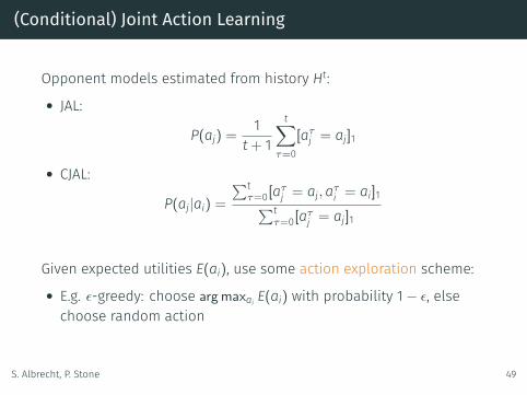
Opponent models estimated from history Ht:
• JAL:
P(aj) =1
t+ 1
t∑τ=0
[aτj = aj]1
• CJAL:
P(aj|ai) =∑t
τ=0[aτj = aj,aτi = ai]1∑tτ=0[aτj = aj]1
Given expected utilities E(ai), use some action exploration scheme:
• E.g. ϵ-greedy: choose argmaxai E(ai) with probability 1− ϵ, elsechoose random action
S. Albrecht, P. Stone 49
(Conditional) Joint Action Learning
Opponent models estimated from history Ht:
• JAL:
P(aj) =1
t+ 1
t∑τ=0
[aτj = aj]1
• CJAL:
P(aj|ai) =∑t
τ=0[aτj = aj,aτi = ai]1∑tτ=0[aτj = aj]1
Given expected utilities E(ai), use some action exploration scheme:
• E.g. ϵ-greedy: choose argmaxai E(ai) with probability 1− ϵ, elsechoose random action
S. Albrecht, P. Stone 49

(Conditional) Joint Action Learning
JAL and CJAL can converge to Nash equilibrium in self-play
CJAL in variant of Prisoner’s Dilemma (from Banerjee and Sen, 2007):
Converging to Pareto-optimal NE (C,C)
S. Albrecht, P. Stone 50

Opponent Modelling
FP, JAL, CJAL are simple examples of opponent modelling:
• Use model of other agent to predict its actions, goals, beliefs, ...
Many forms of opponent modelling exist:• Policy reconstruction• Type-based methods• Classification• Plan recognition
• Recursive reasoning• Graphical methods• Group modelling• ...
Upcoming survey by S. Albrecht & P. Stone!
S. Albrecht, P. Stone 51

Minimax/Nash/Correlated Q-Learning
Minimax Q-Learning (Minimax-Q) (Littman, 1994) andNash Q-Learning (Nash-Q) (Hu and Wellman, 2003) andCorrelated Q-Learning (CE-Q) (Greenwald and Hall, 2003)learn joint-action Q-values for each agent j ∈ N:
Qt+1j (st,at) = (1− α)Qtj(st,at) + α[utj + γEQj(st+1)
]
• Assumes utilities utj are commonly observed• EQ(st+1) is expected utility to agent j under equilibrium profile fornormal-form game with utility functions uj(a) = Qtj(st+1,a)⇒ Minimax-Q: use minimax profile (assumes zero-sum game)⇒ Nash-Q: use Nash equilibrium⇒ CE-Q: use correlated equilibrium
S. Albrecht, P. Stone 52

Minimax/Nash/Correlated Q-Learning
Minimax Q-Learning (Minimax-Q) (Littman, 1994) andNash Q-Learning (Nash-Q) (Hu and Wellman, 2003) andCorrelated Q-Learning (CE-Q) (Greenwald and Hall, 2003)learn joint-action Q-values for each agent j ∈ N:
Qt+1j (st,at) = (1− α)Qtj(st,at) + α[utj + γEQj(st+1)
]• Assumes utilities utj are commonly observed
• EQ(st+1) is expected utility to agent j under equilibrium profile fornormal-form game with utility functions uj(a) = Qtj(st+1,a)⇒ Minimax-Q: use minimax profile (assumes zero-sum game)⇒ Nash-Q: use Nash equilibrium⇒ CE-Q: use correlated equilibrium
S. Albrecht, P. Stone 52

Minimax/Nash/Correlated Q-Learning
Minimax Q-Learning (Minimax-Q) (Littman, 1994) andNash Q-Learning (Nash-Q) (Hu and Wellman, 2003) andCorrelated Q-Learning (CE-Q) (Greenwald and Hall, 2003)learn joint-action Q-values for each agent j ∈ N:
Qt+1j (st,at) = (1− α)Qtj(st,at) + α[utj + γEQj(st+1)
]• Assumes utilities utj are commonly observed• EQ(st+1) is expected utility to agent j under equilibrium profile fornormal-form game with utility functions uj(a) = Qtj(st+1,a)⇒ Minimax-Q: use minimax profile (assumes zero-sum game)⇒ Nash-Q: use Nash equilibrium⇒ CE-Q: use correlated equilibrium
S. Albrecht, P. Stone 52

Minimax/Nash/Correlated Q-Learning
Minimax-Q, Nash-Q, CE-Q can converge to equilibrium in self-play
• E.g. Nash-Q formal proof of convergence to NE• But based on strong restrictions on Qtj !
HU AND WELLMAN
Assumption 3 One of the following conditions holds during learning.3Condition A. Every stage game (Q1t (s), . . . ,Qn
t (s)), for all t and s, has a global optimal point,and agents’ payoffs in this equilibrium are used to update their Q-functions.Condition B. Every stage game (Q1t (s), . . . ,Qn
t (s)), for all t and s, has a saddle point, andagents’ payoffs in this equilibrium are used to update their Q-functions.
We further define the distance between two Q-functions.
Definition 15 For Q, Q 2Q, define
k Q� Q k ⌘ maxjmaxsk Qj(s)� Q j(s) k( j,s)
⌘ maxjmaxsmaxa1,...,an
|Qj(s,a1, . . . ,an)� Q j(s,a1, . . . ,an)|.
Given Assumption 3, we can establish that Pt is a contraction mapping operator.
Lemma 16 k PtQ�PtQ k β k Q� Q k for all Q, Q 2Q.
Proof.
k PtQ�PtQ k = maxjk PtQj�PtQ j k( j)
= maxjmaxs
| βπ1(s) · · ·πn(s)Qj(s)�βπ1(s) · · · πn(s)Q j(s) |
= maxjβ | π1(s) · · ·πn(s)Qj(s)� π1(s) · · · πn(s)Q j(s) |
We proceed to prove that
|π1(s) · · ·πn(s)Qj(s)� π1(s) · · · πn(s)Q j(s)|k Qj(s)� Q j(s) k .
To simplify notation, we use σ j to represent π j(s), and σ j to represent π j(s). The proposition wewant to prove is
|σ jσ� jQ j(s)� σ jσ� jQ j(s)|k Qj(s)� Q j(s) k .
Case 1: Suppose both (σ1, . . . ,σn) and (σ1, . . . , σn) satisfy Condition A in Assumption 3, whichmeans they are global optimal points.
If σ jσ� jQ j(s)� σ jσ� jQ j(s), we have
σ jσ� jQ j(s)� σ jσ� jQ j(s) σ jσ� jQ j(s)�σ jσ� jQ j(s)= ∑
a1,...,anσ1(a1) · · ·σn(an)
�
Qj(s,a1, . . . ,an)� Q j(s,a1, . . . ,an)�
∑a1,...,an
σ1(a1) · · ·σn(an) k Qj(s)� Q j(s) k (15)
= k Qj(s)� Q j(s) k,3. In our statement of this assumption in previous writings (Hu and Wellman, 1998, Hu, 1999), we neglected to includethe qualification that the same condition be satisfied by all stage games. We have made the qualification more explicitsubsequently (Hu and Wellman, 2000). As Bowling (2000) has observed, the distinction is essential.
1050
(Hu and Wellman, 2003)
S. Albrecht, P. Stone 53

Model-Free Learning
JAL, CJAL, Nash-Q, ... learn models of other agents
• Model-based learning
Can also learn without modelling other agents
• Model-free learning• e.g. WoLF-PHC, Regret Matching
S. Albrecht, P. Stone 54

Model-Free Learning
JAL, CJAL, Nash-Q, ... learn models of other agents
• Model-based learning
Can also learn without modelling other agents
• Model-free learning• e.g. WoLF-PHC, Regret Matching
S. Albrecht, P. Stone 54
Win or Learn Fast Policy Hill Climbing
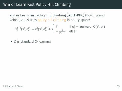
Win or Learn Fast Policy Hill Climbing (WoLF-PHC) (Bowling andVeloso, 2002) uses policy hill climbing in policy space:
πt+1i (st,ati) = πti (st,ati) +{
δ if ati = argmaxa′i Q(st,a′i)
− δ|Ai|−1 else
• Q is standard Q-learning
Variable learning rate δ:
δ =
{δw if
∑ai π
ti (st,ai)Q(st,ai) >
∑ai πi(s
t,ai)Q(st,ai)δl else
• adapt slowly when “winning”, fast when “losing” (δw < δl)• πi is average policy over past policies πi
S. Albrecht, P. Stone 55

Win or Learn Fast Policy Hill Climbing
WoLF gradient ascent in self-play converges to Nash equilibrium intwo-player, two-action repeated game (Bowling and Veloso, 2002)
0
0.2
0.4
0.6
0.8
1
0 200000 400000 600000 800000 1e+06
Pr(H
eads
)
Iterations
WoLF-PHC: Pr(Heads)PHC: Pr(Heads)
0
0.2
0.4
0.6
0.8
1
0 0.2 0.4 0.6 0.8 1
Pr(Paper)
Pr(Rock)
PHCWoLF
(a) Matching Pennies Game (b) Rock-Paper-Scissors Game
Figure 2: (a) Results for matching pennies: the policy for one of the players as a probability distribution while learning withPHC and WoLF-PHC. The other player’s policy looks similar. (b) Results for rock-paper-scissors: trajectories of one player’spolicy. The bottom-left shows PHC in self-play, and the upper-right shows WoLF-PHC in self-play.
and the other trying to move North. Hence the game requiresthat the players coordinate their behaviors.WoLF policy hill-climbing successfully converges to one
of these equilibria. Figure 3(a) shows an example trajectoryof the players’ strategies for the initial state while learningover 100,000 steps. In this example the players convergedto the equilibrium where player one moves East and playertwo moves North from the initial state. This is evidence thatWoLF policy hill-climbing can learn an equilibrium even in ageneral-sum game with multiple equilibria.
5.3 SoccerThe final domain is a comparatively large zero-sum soccergame introduced by Littman [1994] to demonstrate Minimax-Q. An example of an initial state in this game is shown in Fig-ure 3(b), where player ’B’ has possession of the ball. The goalis for the players to carry the ball into the goal on the oppositeside of the field. The actions available are the four compassdirections and the option to not move. The players select ac-tions simultaneously but they are executed in a random order,which adds non-determinism to their actions. If a player at-tempts to move to the square occupied by its opponent, thestationary player gets possession of the ball, and the movefails. Unlike the grid world domain, the Nash equilibrium forthis game requires a mixed policy. In fact any deterministicpolicy (therefore anything learned by an single-agent learneror JAL) can always be defeated [Littman, 1994].Our experimental setup resembles that used by Littman
in order to compare with his results for Minimax-Q. Eachplayer was trained for one million steps. After training,its policy was fixed and a challenger using Q-learning wastrained against the player. This determines the learned pol-icy’s worst-case performance, and gives an idea of how closethe player was to the equilibrium policy, which would per-form no worse than losing half its games to its challenger.Unlike Minimax-Q, WoLF-PHC and PHC generally oscillatearound the target solution. In order to account for this in theresults, training was continued for another 250,000 steps and
evaluated after every 50,000 steps. The worst performing pol-icy was then used for the value of that learning run.Figure 3(b) shows the percentage of games won by the
different players when playing their challengers. “Minimax-Q” represents Minimax-Q when learning against itself (theresults were taken from Littman’s original paper.) “WoLF”represents WoLF policy hill-climbing learning against itself.“PHC(L)” and “PHC(W)” represents policy hill-climbingwith � = �l and � = �w, respectively. “WoLF(2x)” representsWoLF policy hill-climbing learning with twice the training(i.e. two million steps). The performance of the policies wereaveraged over fifty training runs and the standard deviationsare shown by the lines beside the bars. The relative orderingby performance is statistically significant.WoLF-PHC does extremely well, performing equivalently
to Minimax-Q with the same amount of training2 and contin-ues to improve with more training. The exact effect of theWoLF principle can be seen by its out-performance of PHC,using either the larger or smaller learning rate. This showsthat the success of WoLF-PHC is not simply due to changinglearning rates, but rather to changing the learning rate at theappropriate time to encourage convergence.
6 ConclusionIn this paper we present two properties, rationality and con-vergence, that are desirable for a multiagent learning algo-rithm. We present a new algorithm that uses a variable learn-ing rate based on the WoLF (“Win or Learn Fast”) princi-ple. We then showed how this algorithm takes large stepstowards achieving these properties on a number and varietyof stochastic games. The algorithm is rational and is shownempirically to converge in self-play to an equilibrium even ingames with multiple or mixed policy equilibria, which previ-ous multiagent reinforcement learners have not achieved.
2The results are not directly comparable due to the use of a dif-ferent decay of the learning rate. Minimax-Q uses an exponentialdecay that decreases too quickly for use with WoLF-PHC.
Targeted optimality: if opponent policy converges, WoLF-PHCconverges to best-response against opponent
S. Albrecht, P. Stone 56

Regret Matching
Regret Matching (RegMat) (Hart and Mas-Colell, 2000) computesconditional regret for not choosing a′i whenever ai was chosen:
R(ai,a′i) =1
t+ 1∑
τ :aτi = ai
ui(a′i ,aτj )− ui(aτ )
Used to modify policy:
πt+1i (ai) =
1µ max[R(aτi ,ai), 0] ai = ati
1−∑
a′i =aτiπt+1i (a′i) ai = ati
• µ > 0 is “inertia” parameter
S. Albrecht, P. Stone 57

Regret Matching
RegMat converges to correlated equilibrium in self-play
Assumes actions commonly observed and utility functions known
• Modified RegMat (Hart and Mas-Colell, 2001) removesassumptions — only observe own action and utilities
R(ai,a′i) =1
t+ 1∑
τ :aτi = a′i
πτi (ai)
πτi (a′i)
uτi −1
t+ 1∑
τ :aτi = ai
uτi
(plus modified policy normalisation)
• Also converges to correlated equilibrium in self-play!
S. Albrecht, P. Stone 58
Learning in Mixed Groups
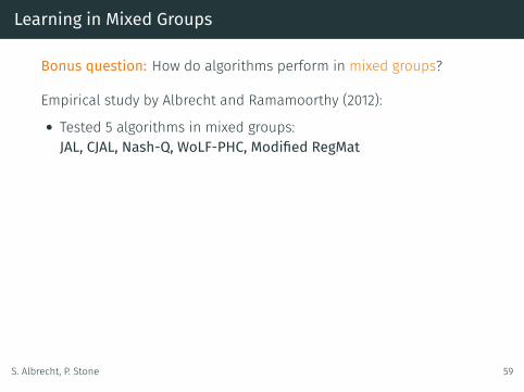
Bonus question: How do algorithms perform in mixed groups?
Empirical study by Albrecht and Ramamoorthy (2012):
• Tested 5 algorithms in mixed groups:JAL, CJAL, Nash-Q, WoLF-PHC, Modified RegMat
• Tested in all (78) structurally distinct, strictly ordinal 2× 2repeated games (Rapoport and Guyer, 1966), e.g.
1,2 2,44,1 3,3
• Also tested in 500 random strictly ordinal 2× 2× 2 (3 agents)repeated games
S. Albrecht, P. Stone 59

Learning in Mixed Groups
Test criteria:• Convergence rate• Final expected utilities• Social welfare/fairness• Solution rates:
• Nash equilibrium (NE)• Pareto-optimality (PO)• Welfare-optimality (WO)• Fairness-optimality (FO)
Which algorithm is best?
S. Albrecht, P. Stone 60

Learning in Mixed Groups
Test criteria:• Convergence rate• Final expected utilities• Social welfare/fairness• Solution rates:
• Nash equilibrium (NE)• Pareto-optimality (PO)• Welfare-optimality (WO)• Fairness-optimality (FO)
Which algorithm is best?
S. Albrecht, P. Stone 60

Learning in Mixed Groups
Conv. Exp. Util. NE PO WO FO
70%
75%
80%
85%
90%
95%
100%Overall results
JALCJALWoLF−PHC RegMat Nash-Q
100% is maximum possible utility/rateDifficulty: NE < PO < WO < FO
S. Albrecht, P. Stone 61

Learning in Mixed Groups
Conv. Exp. Util. NE PO WO FO
70%
75%
80%
85%
90%
95%
100%Overall results
JALCJALWoLF−PHC RegMat Nash-Q
Answer:No clear winner!
S. Albrecht, P. Stone 61

Overview
Introduction
Multiagent Models & Assumptions
Learning Goals
Learning Algorithms
Recent Trends
S. Albrecht, P. Stone 62

Teamwork
Typical approach:
• Whole team designed and trained by single organisation• Agents share coordination protocols, communication languages,domain knowledge, algorithms, ...
⇒ Pre-coordination!
S. Albrecht, P. Stone 63

Teamwork
Typical approach:
• Whole team designed and trained by single organisation• Agents share coordination protocols, communication languages,domain knowledge, algorithms, ...⇒ Pre-coordination!
S. Albrecht, P. Stone 63

Ad Hoc Teamwork
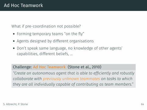
What if pre-coordination not possible?
• Forming temporary teams “on the fly”• Agents designed by different organisations• Don’t speak same language, no knowledge of other agents’capabilities, different beliefs, ...
Challenge: Ad Hoc Teamwork (Stone et al., 2010)“Create an autonomous agent that is able to efficiently and robustlycollaborate with previously unknown teammates on tasks to whichthey are all individually capable of contributing as team members.”
S. Albrecht, P. Stone 64

Ad Hoc Teamwork
What if pre-coordination not possible?
• Forming temporary teams “on the fly”
• Agents designed by different organisations• Don’t speak same language, no knowledge of other agents’capabilities, different beliefs, ...
Challenge: Ad Hoc Teamwork (Stone et al., 2010)“Create an autonomous agent that is able to efficiently and robustlycollaborate with previously unknown teammates on tasks to whichthey are all individually capable of contributing as team members.”
S. Albrecht, P. Stone 64

Ad Hoc Teamwork
What if pre-coordination not possible?
• Forming temporary teams “on the fly”• Agents designed by different organisations
• Don’t speak same language, no knowledge of other agents’capabilities, different beliefs, ...
Challenge: Ad Hoc Teamwork (Stone et al., 2010)“Create an autonomous agent that is able to efficiently and robustlycollaborate with previously unknown teammates on tasks to whichthey are all individually capable of contributing as team members.”
S. Albrecht, P. Stone 64

Ad Hoc Teamwork
What if pre-coordination not possible?
• Forming temporary teams “on the fly”• Agents designed by different organisations• Don’t speak same language, no knowledge of other agents’capabilities, different beliefs, ...
Challenge: Ad Hoc Teamwork (Stone et al., 2010)“Create an autonomous agent that is able to efficiently and robustlycollaborate with previously unknown teammates on tasks to whichthey are all individually capable of contributing as team members.”
S. Albrecht, P. Stone 64

RoboCup Drop-In Competition
RoboCup SPL Drop-In Competition ’13, ’14, ’15 (Genter et al., 2017)
• Mixed players from different teams• No prior coordination between players
Video: Drop-In Competition
S. Albrecht, P. Stone 65

Learning in Ad Hoc Teamwork
Many learning algorithms not suitable for ad hoc teamwork:
• RL-based algorithms (JAL, CJAL, Nash-Q, ...) need 1000’s ofiterations in simple gamesAd hoc teamwork: not much time for learning, trial & error, ...
• Many algorithms designed for self-play (all agents use samealgorithm)Ad hoc teamwork: no control over other agents
Need method which can learn quickly to interact effectively withunknown other agents!
S. Albrecht, P. Stone 66

Type-Based Method
Hypothesise possible types of other agents:
• Each type θj is blackbox behaviour specification:
P(aj|Ht, θj)
• Generate types from e.g.• experience from past interactions• domain and task knowledge• learn new types online (opponent modelling)
S. Albrecht, P. Stone 67

Type-Based Method
Hypothesise possible types of other agents:
• Each type θj is blackbox behaviour specification:
P(aj|Ht, θj)
• Generate types from e.g.• experience from past interactions• domain and task knowledge• learn new types online (opponent modelling)
S. Albrecht, P. Stone 67

Type-Based Method
During the interaction:• Compute belief over types based on interaction history Ht:
P(θj|Ht) ∝ P(Ht|θj)P(θj)
• Plan own action based on beliefs
S. Albrecht, P. Stone 68

Type-Based Method – Planning
Harsanyi-Bellman Ad Hoc Coordination (HBA) (Albrecht et al., 2016)
πi(Ht,ai) ∼ argmaxai
Eaist (Ht)
Eais (H) =∑θj
P(θj|H)∑aj
P(aj|H, θj)Q(ai,aj)s (H)
Qas (H) =∑s′T(s,a, s′)
[ui(s,a) + γmax
aiEais′
(⟨H,a, s′⟩
)]
Optimal planning with built-in exploration: Value of Information
S. Albrecht, P. Stone 69

Type-Based Method – Planning
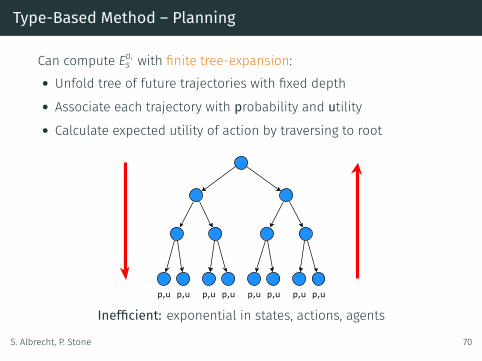
Can compute Eais with finite tree-expansion:• Unfold tree of future trajectories with fixed depth• Associate each trajectory with probability and utility• Calculate expected utility of action by traversing to root
Inefficient: exponential in states, actions, agents
S. Albrecht, P. Stone 70
Type-Based Method – Planning
Can compute Eais with finite tree-expansion:• Unfold tree of future trajectories with fixed depth• Associate each trajectory with probability and utility• Calculate expected utility of action by traversing to root
Inefficient: exponential in states, actions, agents
S. Albrecht, P. Stone 70

Type-Based Method – Planning
Use Monte-Carlo Tree Search (MCTS) for efficient approximation:
Repeat x times:1. Sample type θj ∈ Θj withprobabilities P(θj|Ht)
2. Sample interaction trajectoryusing θj and domain model T
3. Update utility estimates viabackprop on trajectory
E.g. Albrecht and Stone (2017), Barrett et al. (2011)
But: loses value of information! (no belief change during planning)
S. Albrecht, P. Stone 71

Ad Hoc Teamwork: Predator Pursuit
4 predators must capture 1 prey in grid world (Barrett et al., 2011)• We control one agent in predator team• Policies of other predators unknown (prey moves randomly)• 4 types provided to our agent; online planning using MCTS
Video: 4 types, true type insideVideo: 4 types, true type outside (students)Source: http://www.cs.utexas.edu/~larg/index.php/Ad_Hoc_Teamwork:_Pursuit
S. Albrecht, P. Stone 72

Ad Hoc Teamwork: Half Field Offense
4 offense players vs. 5 defense players (Barrett and Stone, 2015)
• We control one agent (green) inoffensive team (yellow)
• Policies of teammates unknown(defense uses fixed policies)
• 7 team types provided to our agent;for each team type, plan own policyoffline using RL
Video: 4v5 Half Field OffenseSource:http://www.cs.utexas.edu/~larg/index.php/Ad_Hoc_Teamwork:_HFO
S. Albrecht, P. Stone 73

Learning Parameters in Types
We can learn more: parameters in types! (Albrecht and Stone, 2017)
P(ai|Ht, θj,p)
• p = (p1, ...,pk) continuous parameter vector• Complex types can have several parameters⇒ learning rate, exploration rate, discount factor, ...
Goal: simultaneously learn type and parameters in type
S. Albrecht, P. Stone 74

Learning Parameters in Types
For each type θj ∈ Θj, maintain parameter estimate p ∈ [pmin,pmax]
S. Albrecht, P. Stone 75
Observe action atj of agent j
Select types Φ ⊂ Θj for updating
For each θj ∈ Φ, update estimate pt → pt+1
Update beliefs:
P(θj|Ht+1) ∝ P(atj |Ht, θj,pt+1)P(θj|Ht)
Plan own action

Updating Parameter Estimates
S. Albrecht, P. Stone 76
Given type θj, updateparameter estimate
pt → pt+1
Type definesaction likelihoods
P(atj |Ht, θj,p) P (a0j |H0, θj , p1, p2)
P (a1j |H1, θj , p1, p2)
-5
P (a2j |H2, θj , p1, p2)
5
p1
0
p2
05 -5

Updating Parameter Estimates
S. Albrecht, P. Stone 77
Bayesian updating:• Approximate P(atj |Ht, θj,p) aspolynomial with variables p
• Perform conjugate updatesthrough successive layers
Global optimisation:
argmaxp
t+1∏τ=1
P(aτ−1j |Hτ−1, θj,p)
Solve with Bayesian optimisation
(Albrecht and Stone, 2017)
P (a0j |H0, θj , p1, p2)
P (a1j |H1, θj , p1, p2)
-5
P (a2j |H2, θj , p1, p2)
5
p1
0
p2
05 -5

Ad Hoc Teamwork: Level-Based Foraging
Blue = our agent, red = other agentsGoal: collect all items in minimal timeAgents can collect item ifsum of agent levels ≥ item level
4 possible types for red, e.g.• search for item, try to load• search for agent, load itemclosest to agent
Each type uses 3 parameters:• skill level, view radius, view angle
Blue doesn’t know true type of red norparameter values of type
0.15
0.58
0.83
0.53
0.23
0.48
0.55
S. Albrecht, P. Stone 78

Ad Hoc Teamwork: Level-Based Foraging
Video: 10x10 world, 2 agents
0.15
0.58
0.83
0.53
0.23
0.48
0.55
Video: 15x15 world, 3 agents
.90
.57
.35
.87.32
.95
.67
.69
.79
.56
.63
.43
.23
S. Albrecht, P. Stone 79

Type-Based Method & Ad Hoc Teamwork
• AAAI’16 Tutorial on Type-Based Methods:http://thinc.cs.uga.edu/tutorials/aaai-16.html
• Special Issue on Multiagent Interaction without Prior Coordination(MIPC): http://mipc.inf.ed.ac.uk/journal
• MIPC Workshops:• AAMAS’17, Sao Paulo, Brazil• AAAI’16, Phoenix, Arizona, USA• AAAI’15, Austin, Texas, USA• AAAI’14, Quebec City, Canada
http://mipc.inf.ed.ac.uk
S. Albrecht, P. Stone 80
Deep Reinforcement Learning
Standard Q-learning assumes tabular representation:
• One entry in Q for each (s,a)
⇒ Does not scale to complex domains!⇒ Does not generalise values!
Needs extra engineering to work, including:
• State abstraction to reduce state space(usually hand-coded & domain-specific)
• Function approximation to store and generalise Q(e.g. linear function approximation in state features)
S. Albrecht, P. Stone 81
Deep Reinforcement Learning
Standard Q-learning assumes tabular representation:
• One entry in Q for each (s,a)⇒ Does not scale to complex domains!
⇒ Does not generalise values!
Needs extra engineering to work, including:
• State abstraction to reduce state space(usually hand-coded & domain-specific)
• Function approximation to store and generalise Q(e.g. linear function approximation in state features)
S. Albrecht, P. Stone 81

Deep Reinforcement Learning
Standard Q-learning assumes tabular representation:
• One entry in Q for each (s,a)⇒ Does not scale to complex domains!⇒ Does not generalise values!
Needs extra engineering to work, including:
• State abstraction to reduce state space(usually hand-coded & domain-specific)
• Function approximation to store and generalise Q(e.g. linear function approximation in state features)
S. Albrecht, P. Stone 81

Deep Reinforcement Learning
New problem: extra engineering may limit performance!• State abstraction may be wrong (e.g. too coarse)• Function approximator may be inaccurate
Idea: deep reinforcement learning• Use “deep” neural network to represent Q• Learn on raw data (no state abstraction)⇒ Let network learn good abstraction on its own!
S. Albrecht, P. Stone 82

Deep Reinforcement Learning
Deep learning: neural network with many layers• Input layer takes raw data→ s• Hidden layers transform data• Output layer returns target scalars→ Q(s, ·)• Train network with back-propagation on labelled data
S. Albrecht, P. Stone 83

Deep Q-Learning
Deep Q-Learning (Mnih et al., 2013)Initialise network parameters Ψ with random weights
1. Observe current state st
2. With probability ϵ, select random action atElse, select action at ∈ argmaxa Q(st,a; Ψ)
3. Get reward rt and new state st+1
4. Store experience (st,at, rt, st+1) in D
5. Sample random minibatch D+ ⊂ D
6. For each (sτ ,aτ , rτ , sτ+1) ∈ D+, perform gradient descent step on
(yτ − Q(sτ ,aτ ; Ψ))2
yτ = rτ + γmaxa′
Q(sτ ,a′; Ψfixed)
S. Albrecht, P. Stone 84
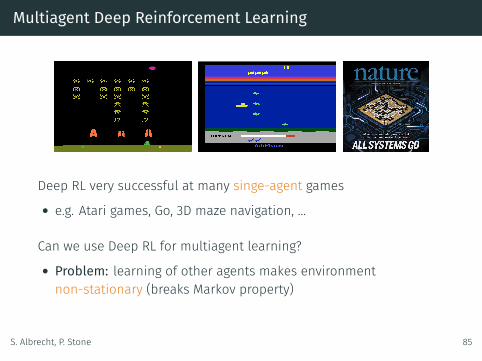
Multiagent Deep Reinforcement Learning
Deep RL very successful at many singe-agent games
• e.g. Atari games, Go, 3D maze navigation, ...
Can we use Deep RL for multiagent learning?
• Problem: learning of other agents makes environmentnon-stationary (breaks Markov property)
S. Albrecht, P. Stone 85

Independent Deep Q-Learners
Video: Cooperative PongVideo: Competitive Pong(Tampuu et al., 2017)
https://www.youtube.com/watch?v=Gb9DprIgdGwhttps://www.youtube.com/watch?v=nn6_GUVDnVw
Video: Gathering gameVideo: Wolfpack game(Leibo et al., 2017)
https://www.youtube.com/watch?v=F97lqqpcqsMhttps://www.youtube.com/watch?v=kXudpMfecs4
Video: Starcraft(Foerster et al., 2017)
https://www.youtube.com/watch?v=RK7y_uQmwhw
S. Albrecht, P. Stone 86

Multiagent Deep Reinforcement Learning
Some recent works on multiagent deep RL:• Emergence of cooperative/competitive behaviours(Tampuu et al., 2017; Leibo et al., 2017)
• Learning communication protocols(Sukhbaatar et al., 2016; Foerster et al., 2016)
• Opponent modelling(He et al., 2016)
• Improved minibatch selection(Palmer et al., 2017; Foerster et al., 2017)
• Multi-task learning(Omidshafiei et al., 2017)
• Learning value decomposition(Sunehag et al., 2017)
S. Albrecht, P. Stone 87

Concluding Remarks
We covered...
• Multiagent models: normal-form games, repeated games,stochastic games, ...
• Learning goals: equilibria, no-regret, targeted optimality, ...• Learning algorithms: internal view, model-based, model-free• Recent trends: ad hoc teamwork, deep RL
Download tutorial slides at:http://www.cs.utexas.edu/~larg/ijcai17_tutorial
Watch out for our upcoming survey on agents modelling otheragents!
S. Albrecht, P. Stone 88

References i
S. Albrecht and S. Ramamoorthy. Comparative evaluation of MAL algorithmsin a diverse set of ad hoc team problems. In Proceedings of the 11thInternational Conference on Autonomous Agents and Multiagent Systems,pages 349–356, 2012.
S. Albrecht and S. Ramamoorthy. A game-theoretic model and best-responselearning method for ad hoc coordination in multiagent systems. Technicalreport, https://arxiv.org/abs/1506.01170, 2013.
S. Albrecht and P. Stone. Reasoning about hypothetical agent behavioursand their parameters. In Proceedings of the 16th International Conferenceon Autonomous Agents and Multiagent Systems, pages 547–555, 2017.
S. Albrecht, J. Crandall, and S. Ramamoorthy. Belief and truth inhypothesised behaviours. Artificial Intelligence, 235:63–94, 2016.
E. Alonso, M. D’Inverno, D. Kudenko, M. Luck, and J. Noble. Learning inmulti-agent systems. Knowledge Engineering Review, 16(3):277–284, 2001.
S. Albrecht, P. Stone 89

References ii
R. Aumann. Subjectivity and correlation in randomized strategies. Journal ofmathematical Economics, 1:67–96, 1974.
B. Banerjee and J. Peng. Performance bounded reinforcement learning instrategic interactions. In Proceedings of the 19th AAAI Conference onArtificial Intelligence, pages 2–7, 2004.
D. Banerjee and S. Sen. Reaching pareto-optimality in prisoner’s dilemmausing conditional joint action learning. Autonomous Agents andMulti-Agent Systems, 15(1):91–108, 2007.
S. Barrett and P. Stone. Cooperating with unknown teammates in complexdomains: A robot soccer case study of ad hoc teamwork. In Proceedings ofthe 29th AAAI Conference on Artificial Intelligence, pages 2010–2016, 2015.
S. Barrett, P. Stone, and S. Kraus. Empirical evaluation of ad hoc teamwork inthe pursuit domain. In Proceedings of the 10th International Conferenceon Autonomous Agents and Multiagent Systems, pages 567–574, 2011.
S. Albrecht, P. Stone 90

References iii
M. Bowling. Convergence and no-regret in multiagent learning. In Advancesin Neural Information Processing Systems, pages 209–216, 2005.
M. Bowling and M. Veloso. Multiagent learning using a variable learning rate.Artificial Intelligence, 136(2):215–250, 2002.
G. Brown. Iterative solution of games by fictitious play. In Proceedings of theConference on Activity Analysis of Production and Allocation, CowlesCommission Monograph 13, pages 374–376, 1951.
L. Busoniu, R. Babuska, and B. De Schutter. A comprehensive survey ofmultiagent reinforcement learning. IEEE Transactions on Systems, Man,and Cybernetics, Part C, 38(2), 2008.
D. Chakraborty and P. Stone. Multiagent learning in the presence ofmemory-bounded agents. Autonomous Agents and Multi-Agent Systems,28(2):182–213, 2014.
S. Albrecht, P. Stone 91

References iv
C. Claus and C. Boutilier. The dynamics of reinforcement learning incooperative multiagent systems. In Proceedings of the 15th NationalConference on Artificial Intelligence, pages 746–752, 1998.
V. Conitzer and T. Sandholm. AWESOME: a general multiagent learningalgorithm that converges in self-play and learns a best response againststationary opponents. Machine Learning, 67(1-2):23–43, 2007.
J. Crandall. Towards minimizing disappointment in repeated games. Journalof Artificial Intelligence Research, 49:111–142, 2014.
A. Fink. Equilibrium in a stochastic n-person game. Journal of Science of theHiroshima University, 28(1):89–93, 1964.
J. Foerster, Y. Assael, N. de Freitas, and S. Whiteson. Learning to communicatewith deep multi-agent reinforcement learning. In Advances in NeuralInformation Processing Systems 29, pages 2137–2145, 2016.
S. Albrecht, P. Stone 92

References v
J. Foerster, N. Nardelli, G. Farquhar, T. Afouras, P. H. S. Torr, P. Kohli, andS. Whiteson. Stabilising experience replay for deep multi-agentreinforcement learning. In Proceedings of the 34th InternationalConference on Machine Learning, pages 1146–1155, 2017.
K. Genter, T. Laue, and P. Stone. Three years of the RoboCup standardplatform league drop-in player competition: Creating and maintaining alarge scale ad hoc teamwork robotics competition. Autonomous Agentsand Multi-Agent Systems, 31(4):790–820, 2017.
A. Greenwald and K. Hall. Correlated Q-learning. In Proceedings of the 20thInternational Conference on Machine Learning, pages 242–249, 2003.
S. Hart and A. Mas-Colell. A simple adaptive procedure leading to correlatedequilibrium. Econometrica, 68(5):1127–1150, 2000.
S. Hart and A. Mas-Colell. A reinforcement procedure leading to correlatedequilibrium. Economic Essays: A Festschrift for Werner Hildenbrand, pages181–200, 2001.
S. Albrecht, P. Stone 93

References vi
H. He, J. Boyd-Graber, K. Kwok, and H. Daumé III. Opponent modeling in deepreinforcement learning. In Proceedings of the 33rd InternationalConference on Machine Learning, pages 1804–1813, 2016.
J. Hu and M. Wellman. Nash Q-learning for general-sum stochastic games.Journal of Machine Learning Research, 4:1039–1069, 2003.
J. Z. Leibo, V. Zambaldi, M. Lanctot, J. Marecki, and T. Graepel. Multi-agentreinforcement learning in sequential social dilemmas. In Proceedings ofthe 16th International Conference on Autonomous Agents and Multi-AgentSystems, pages 464–473, 2017.
M. Littman. Markov games as a framework for multi-agent reinforcementlearning. In Proceedings of the 11th International Conference on MachineLearning, pages 157–163, 1994.
M. Littman. Friend-or-foe Q-learning in general-sum games. In Proceedingsof the 18th International Conference on Machine Learning, pages 322–328,2001.
S. Albrecht, P. Stone 94

References vii
V. Mnih, K. Kavukcuoglu, D. Silver, A. Graves, I. Antonoglou, D. Wierstra, andM. Riedmiller. Playing Atari with deep reinforcement learning. arXivpreprint arXiv:1312.5602, 2013.
J. Nash. Equilibrium points in n-person games. Proceedings of the NationalAcademy of Sciences, 36(1):48–49, 1950.
S. Omidshafiei, J. Pazis, C. Amato, J. P. How, and J. Vian. Deep decentralizedmulti-task multi-agent reinforcement learning under partial observability.In International Conference on Machine Learning, pages 2681–2690, 2017.
G. Palmer, K. Tuyls, D. Bloembergen, and R. Savani. Lenient multi-agent deepreinforcement learning. arXiv preprint arXiv:1707.04402, 2017.
L. Panait and S. Luke. Cooperative multi-agent learning: The state of the art.Autonomous Agents and Multi-Agent Systems, 11(3):387–434, 2005.
A. Rapoport and M. Guyer. A taxonomy of 2× 2 games. General Systems:Yearbook of the Society for General Systems Research, 11:203–214, 1966.
S. Albrecht, P. Stone 95

References viii
S. Sen and G. Weiss. Learning in multiagent systems. In Multiagent Systems:A Modern Approach to Distributed Artificial Intelligence, chapter 6, pages259–298. MIT Press, 1999.
L. Shapley. Stochastic games. Proceedings of the National Academy ofSciences, 39(10):1095–1100, 1953.
Y. Shoham, R. Powers, and T. Grenager. Multi-agent reinforcement learning: Acritical survey. Unpublished survey, 2003.
P. Stone and M. Veloso. Multiagent systems: A survey from a machinelearning perspective. Autonomous Robots, 8(3):345–383, 2000.
P. Stone, R. S. Sutton, and G. Kuhlmann. Reinforcement learning for RoboCupsoccer keepaway. Adaptive Behavior, 13(3):165–188, 2005.
P. Stone, G. Kaminka, S. Kraus, and J. Rosenschein. Ad hoc autonomous agentteams: collaboration without pre-coordination. In Proceedings of the 24thAAAI Conference on Artificial Intelligence, pages 1504–1509, 2010.
S. Albrecht, P. Stone 96

References ix
S. Sukhbaatar, A. Szlam, and R. Fergus. Learning multiagent communicationwith backpropagation. In Advances in Neural Information ProcessingSystems 29, pages 2244–2252, 2016.
P. Sunehag, G. Lever, A. Gruslys, W. Czarnecki, V. Zambaldi, M. Jaderberg,M. Lanctot, N. Sonnerat, J. Leibo, K. Tuyls, and T. Graepel.Value-decomposition networks for cooperative multi-agent learning. arXivpreprint arXiv:1706.05296, 2017.
A. Tampuu, T. Matiisen, D. Kodelja, I. Kuzovkin, K. Korjus, J. Aru, J. Aru, andR. Vicente. Multiagent cooperation and competition with deepreinforcement learning. PloS ONE, 12(4):e0172395, 2017.
K. Tuyls and G. Weiss. Multiagent learning: Basics, challenges, and prospects.AI Magazine, 33(3):41, 2012.
J. von Neumann and O. Morgenstern. Theory of Games and EconomicBehavior. Princeton University Press, 1944.
S. Albrecht, P. Stone 97

References x
X. Wang and T. Sandholm. Reinforcement learning to play an optimal Nashequilibrium in team Markov games. In Advances in Neural InformationProcessing Systems 15, pages 1603–1610, 2003.
S. Albrecht, P. Stone 98