Multi Variable Loop Shaping

EL2520 Control Theory and Practice Elling W Jacobsen [email protected]

EL2520Control Theory and Practice

Lecture 7:

Multivariable loop shaping

Elling W Jacobsen

School of Electrical Engineering

KTH, Stockholm, Sweden


Course structure

Three parts

1. SISO control revisited

2. Multivariable control

a. Multivariable linear systems

b. Multivariable loop shaping (today)

c. Linear quadratic control

d. H2, H1 and design example

e. Decentralized control and decoupling

f. Glover-McFarlane loop shaping

3. Systems with hard constraints


Multivariable systems cont’d

Last lecture…

• Transfer matrices and block diagram manipulations (order matters!)

• Poles and zeros of multivariable systems (from transfer matrices)

• System gain and amplification (directions matter!)

…continued this lecture

• Recap of last lecture

• Fundamental limitations and robustness of MIMO systems

• Modern multivariable loop shaping


The multivariable frequency response

For a linear multivariable system Y(s)=G(s)U(s), we have

We can bound the amplification at any frequency using

with equality if U(i) parallell w. corresponding input singular vector.


The multivariable frequency response

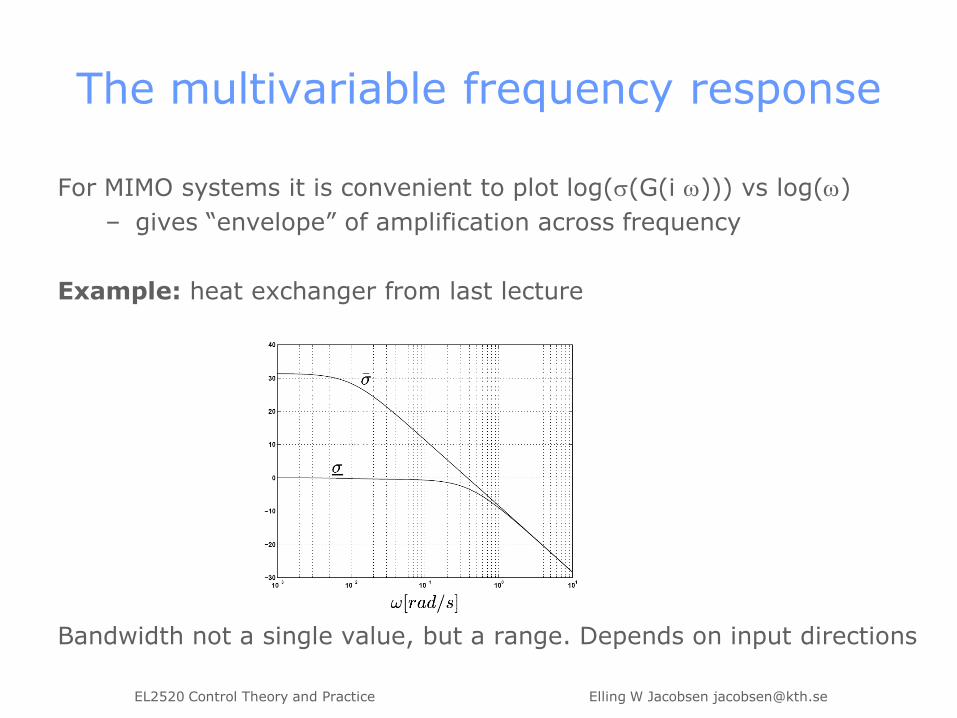
For MIMO systems it is convenient to plot log((G(i ))) vs log()

– gives “envelope” of amplification across frequency

Example: heat exchanger from last lecture

Bandwidth not a single value, but a range. Depends on input directions


Multivariable (open-) loop shaping

Similar reasoning as in SISO case gives requirements on GFy

Note: should push up smallest singular value at low frequencies, and

make sure that largest singular value is small at high frequencies.


As for scalar systems, we get

where

Note: the infinity norm computes the maximum amplifications

across frequency (sup) and input directions ( )

The system gain


Poles and zeros of MIMO systems

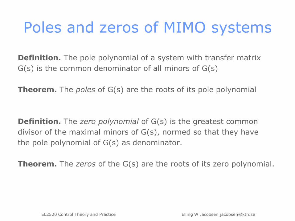
Definition. The pole polynomial of a system with transfer matrix

G(s) is the common denominator of all minors of G(s)

Theorem. The poles of G(s) are the roots of its pole polynomial

Definition. The zero polynomial of G(s) is the greatest common

divisor of the maximal minors of G(s), normed so that they have

the pole polynomial of G(s) as denominator.

Theorem. The zeros of the G(s) are the roots of its zero polynomial.


Notes on poles and zeros

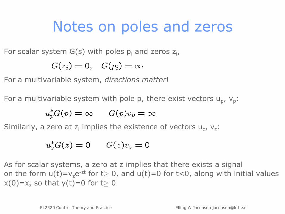
For scalar system G(s) with poles pi and zeros zi,

For a multivariable system, directions matter!

For a multivariable system with pole p, there exist vectors up, vp:

Similarly, a zero at zi implies the existence of vectors uz, vz:

As for scalar systems, a zero at z implies that there exists a signal

on the form u(t)=vze-zt for t¸ 0, and u(t)=0 for t<0, along with initial values

x(0)=xz so that y(t)=0 for t¸ 0


Example: RHP zeros

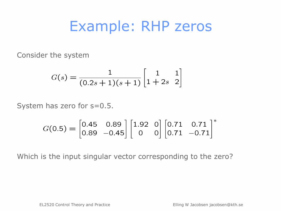
Consider the system

System has zero for s=0.5.

Which is the input singular vector corresponding to the zero?


Example: RHP zeros cont’dStep responses for (u1, u2)=(1,0), (0,1) and (1,-1)

0 2 4 6 8 10-1

0

1

2

(u1,

u2)=

(1,

0)

y1(green) and y

2(blue)

0 2 4 6 8 10-1

0

1

2

(u1,

u2)=

(0,

1)

0 2 4 6 8 10-1

0

1

2

(u1, u

2)=

(1, -1

) Clear non-minimum phase behavior!


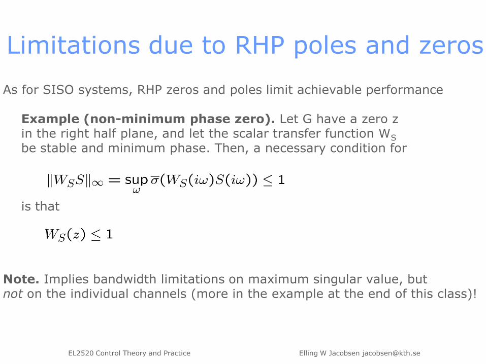
Limitations due to RHP poles and zeros

As for SISO systems, RHP zeros and poles limit achievable performance

Example (non-minimum phase zero). Let G have a zero zin the right half plane, and let the scalar transfer function WS

be stable and minimum phase. Then, a necessary condition for

is that

Note. Implies bandwidth limitations on maximum singular value, butnot on the individual channels (more in the example at the end of this class)!


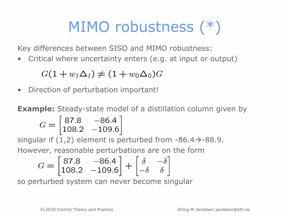
MIMO robustness (*)

Key differences between SISO and MIMO robustness:

• Critical where uncertainty enters (e.g. at input or output)

• Direction of perturbation important!

Example: Steady-state model of a distillation column given by

singular if (1,2) element is perturbed from -86.4-88.9.

However, reasonable perturbations are on the form

so perturbed system can never become singular


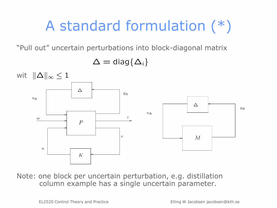
“Pull out” uncertain perturbations into block-diagonal matrix

with

Note: one block per uncertain perturbation, e.g. distillationcolumn example has a single uncertain parameter.

A standard formulation (*)


The structured singular value (*)

Conservative to use small gain, e.g. require that

The structured singular value: find smallest structured perturbation

(in terms of ) that renders closed-loop unstable, i.e. causes

Then, the structured singular value

Powerful framework for analysis and design of robust MIMO controllers

• Details out of the scope of this course

• Learn more in our graduate (PhD-level) course on robust control!


Multivariable systems cont’d

Last lecture…

• Transfer matrices and block diagram manipluations (order matters!)

• System gain and amplification (directions matter!)

• Poles and zeros of multivariable systems (from transfer matrices)

…continued on this lecture

• Recap of last lecture

• Fundamental limitations and robustness of MIMO systems

• Modern multivariable loop shaping


Mixed sensitivity design

Note: Now, WS are matrices, constraints on maximum singular values

Forbidden area

Forbidden area

Convenient to design controller by constraining critical transfer matrices


Approximate design specifications

Problem: find controller that satisfies specifications

Computationally more convenient to use the approximate form

Can be viewed as the norm of an extended system


The extended system


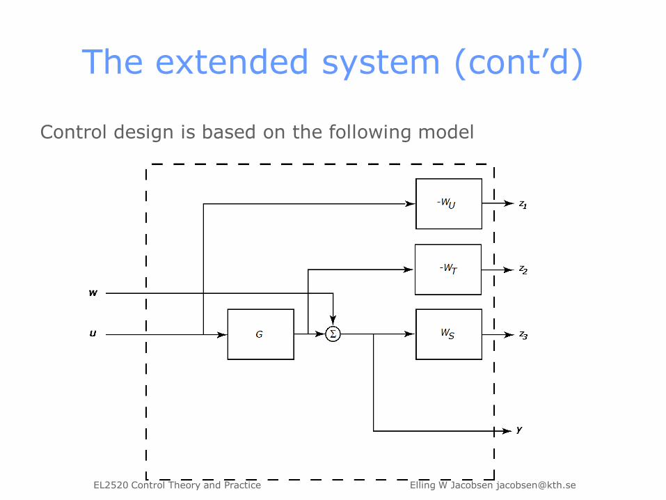
The extended system (cont’d)

Control design is based on the following model


The control design problem

Find controller that minimizes (some) norm of closed-loop

system from w to z,

Model:

Assumption:

Note: Dynamics of weights WS, WT, WU part of system dynamics.


H1 optimal control

Finding a controller that satisfies

can be done by solving a Riccati equation

with =1. If solution P satisfies P¸ 0, A-BBTP stable, the controller

fulfills the specifications (note: observer+state feedback)


How to select weights

Useful to constrain weights, limit number of ”tuning knobs” in design

1. Start with scalar weights (only use matrix-weights when needed).Make sure weights are stable and minimum phase (why?)

2. Use simple weights with easy interpretation.

Ex.

3. Start shaping most important transfer matrix, then add one by one

Ex.

4. When channels are very different, use diagonal weights


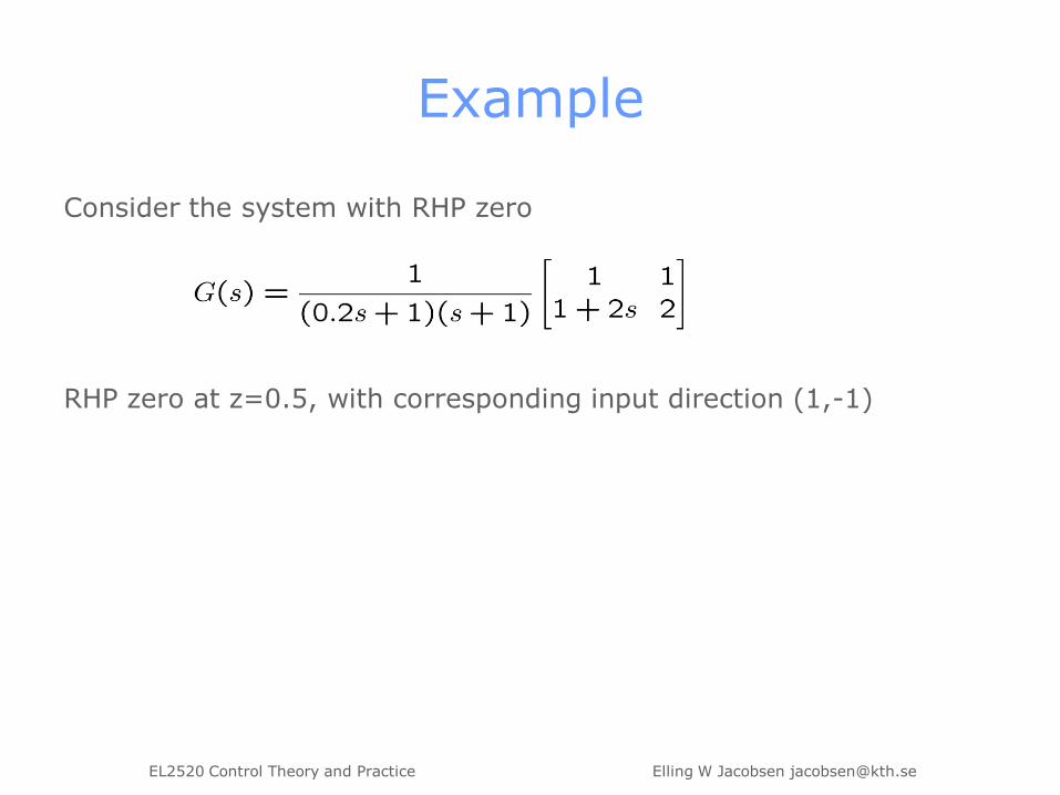
Example

Consider the system with RHP zero

RHP zero at z=0.5, with corresponding input direction (1,-1)


A first design…

Since system has RHP zero at z=0.5, a reasonable weight is

The mixed sensitivity design achieves min=2.79.

Reasonable sensitivities, but poor time-domain performance.


A second design…

Can shift bandwidth limitation from one channel to the other

(i.e. alter singular vectors; limitation on maximum singular value remains)

Time response on channel two much better, constraint on bandwidth

of maximum singular value of S still present.


Conclusions

More elements of multivariable system theory

• Multivariable frequency responses, gains, poles/zeros, directions

Key concepts from SISO analysis carry over

• fundamental limitations, robustness, loop shaping

Modern loop shaping

• Mixed sensitivity design: minimizing H1 norm of extended system

• Optimal solution is state-feedback plus observer

• Tuning knobs for design are weight functions

• Weight selection: part art, part science (must practice!)

Multi Variable Loop Shaping

Documents

Transcript of Multi Variable Loop Shaping