MULTI-SWIRLER AERODYNAMICS: COMPARISON OF …

1 Copyright © 2002 by ASME

Proceedings of ASME Turbo Expo 2002

June 3-6, 2002, Amsterdam, The Netherlands

GT-2002-30464

MULTI-SWIRLER AERODYNAMICS: COMPARISON OF DIFFERENT CONFIGURATIONS

J. Cai and S.-M. Jeng, Univ. of Cincinnati, Cincinnati, OH

R. Tacina NASA, Glenn Research Center, Cleveland, OH

ABSTRACT The non-reacting fluid flow fields generated by multi-

swirler arrays with two different port configurations were investigated experimentally. These two cases include a co-swirling array, where all swirlers act in the same direction, and a counter-swirling array, where all swirlers alternate between clockwise and counter-clockwise rotations. Each configuration consists of a three by three arrangement of swirlers, which use analogous geometries to generate the swirling flows, i.e. eight discrete jets. For each array, the mean and turbulence velocities were measured at approximately 25,000 discrete spatial locations by a two-component LDV system. Furthermore, the third velocity component was derived based on the symmetric geometry of the arrays. In both cases, the coalescence distance, distance for eight discrete jet streams to form uniform swirling flows, is very short; and each swirler within the arrangement possesses a central recirculation zone. These nine zones have varying strengths depending on the individual swirler location, and some rotate with the swirler direction. In comparison, the co-swirler configuration provides a large unified rotational flow in the same direction as the individual swirlers, while a counter-rotating flow pattern is formed by the other case. Lastly, interactions between the unified flow with that of each swirler in the array are discussed and further comparisons are made between the two cases.

INTRODUCTION

Low pollutant emissions are an essential characteristic for a modern gas turbine. Moreover, the economics of gas turbine design demand high-pressure ratios and high turbine inlet temperatures increasing engine cycle efficiency and, thusly, reducing the specific fuel consumption. However, higher pressure and temperature combustors produce an increasing amount of nitrogen oxide (NOx) emissions contradicting this vital low pollutant characteristic.

To achieve a favorable balance, decreasing either the flame temperature or the flow residence time presents two popular and effective approaches to reducing NOx emissions. One recently suggested method of attaining substantially lower NOx emissions for high overall pressure ratio aircraft gas

turbines is the advanced multi-point Lean Direct Injection (LDI) methodology [1]. As shown in Figure 1, multiple smaller-sized swirlers are employed to diminish the possibility of non-uniform combustion caused by direct fuel injection. In addition, these smaller swirlers reduce the required combustor length to have complete air/fuel mixing. As a result, the LDI concept decreases the combustion zone temperature and the flow residence time, thereby lowering pollutant emissions. Furthermore, a lesser amount of necessary airflow for liner cooling leading to the shorter combustor length and therefore less structural weight.

The gas turbine industry widely uses swirling air flow inside combustors for flame stabilization and improved air/fuel mixing. In attempts to further industry development, many individuals, such as Beer, Gupta, and Lilley, have discussed different methods of rotational flow generation inside the combustors and their respective aerodynamic characteristics [2-4]. Specifically, Ahamed investigated the velocity and turbulence of isothermal swirling flows [5]. Furthermore, Bach and Gouldin , Gouldin et al , Ramos and Somer , and Halpin studied the aerodynamics associated with co-axial flow swirlers [6-9]. Finally, Wang et al studied the interactions between co-axial swirlers and individual liquid droplets [10-12]. However, these studies have yet to be extrapolated to multi-swirler array.

In a previous paper [13], the aerodynamics of a co-swirling injector array was studied experimentally. From this previous experiment, the mean velocity and turbulent characteristics of a single three-by-three swirler array were reported. The objective of this paper is to compare the flow structures generated by two differently configured swirler arrays, one with co-swirling ports where all swirlers have the same rotation and one with counter-swirling ports where all swirlers alternate between clockwise and counter-clockwise rotations. Within both configurations, each individual swirler utilizes a similar geometry, i.e. eight discrete jets, to create the rotational fluid flows. This paper reports graphical results from experimental measurements conducted on each configuration of prototype LDI swirler arrays.


EXPERIMENTAL SET-UP As illustrated in Figure 2, the swirler arrays possess a

modular construction consisting of a mounting flange, a swirler holding plate, and nine swirlers. The mounting flange connects to the swirler holding plate to the air supply system, and the swirlers are assembled to the holding plate in the proper configurations. For the co-swirler arrangement, all of the swirlers have the same rotating directions as shown in Figure 3(a). Alternatively, the counter-swirler arrangement, neighboring swirlers have opposite rotating direction illustrated in Figure 3(b). Individual swirlers contain eight 0.125-inch drilled holes around a 0.500-inch diameter, each with a 35-degree tilt angle relative to the longitudinal axis of the swirler.

A schematic of the experiment arrangement, shown in Figure 4, includes a pneumatic system consisting of a 160 cfm at 120 psi compressor, a 30° F dew point dryer, a 0.5-micron particle filter, a pressure regulator, and a 200-gallon air storage tank. An ASME orifice flow meter is utilized to measure airflow rate into the system. Then, the air passes through a, which contains a honeycomb flow conditioner and is instrumented with a thermocouple and pressure probe to measure test conditions, and leads into a test section with internal dimensions of 3×3×12 in3 constructed of thin Plexiglas.

A TSI two-component LDV system is used to measure the axial velocity component and one horizontal velocity component. Also depicted in Figure 4, this LDV system consists of a 3 W argon laser, an optical fiber drive, a transmitter, a receiver, two photomultipliers, and RSA signal processors. The 500mm-focus length transmitter and the 300mm-focus length receiver are mounted on a computer-controlled 3-D traverse. Furthermore, a TSI six-jet aerosol generator provides 3-micron seeding particles for the LDV measurements. The forward scatter mode of the measuring system was employed in order to achieve the best signal-to-noise ratio.

Measurements are taken under environment temperature (20°C) and the pressure drop between the air manifold and surrounding environment is 4% of atmosphere pressure. Measurements were conducted along the twelve cross-sections downstream of each swirler array, illustrated in Figure 5. The data-sampling rate of a typical measurement is controlled to 600 Hz.; and the reported time-averaged data is based on 3000 data points collected at each measuring location during a 5-second period. This procedure is repeated at every node of a 1 mm square grid (approximately 2500 locations) for the first five axial cross-sections from the array, i.e. up to 13 mm, and every node of a 2 mm square grid thereafter (approximately 650 locations). Taking advantage of the inherent symmetric geometry, only 44.4% (4/9) of the total area is measured at each axial cross-section, depicted by the shaded region in Figure 3. Moreover, the nine swirlers are grouped into three types, labeled A, B and C in Figure 3, according to their geometric locations; and each type behaves similarly according to the symmetry of the hardware.

Labeling the axial direction as “z” and the two horizontal directions as “x” and “y” illustrated in Figure 6, the

origin of the coordinate system is located at the center of the central A swirler. The axial velocity and one horizontal velocity component in the x-direction are measured directly from the LDV system. Then, the third velocity component in the y-direction is derived mathematically from the symmetric geometry as shown in Figure 6. Using the center of the test section as the origin, the x- and y-direction velocity components of two positions, symmetrical relative to the diagonal line, are the same. Specifically, V1 = -U2 and V2 = -U1 for each two positions symmetric relative to the diagonal. However, manufacturing imperfections, misalignment of the hardware, and inaccuracy of the LDV probe positions can cause inaccuracies of the derived y-direction velocity component.

RESULT AND DISCUSSION

Mean Axial Velocity

As shown in Figure 7(a) for co-rotational and Figure

7(b) for counter-rotational swirlers, the axial mean velocity contours at 3 mm downstream are similar. Four types of flow patterns are found at this position. First, each set of eight jets with maximum axial velocities of about 50 m/s form the jet zones characterized by an annulus shape with positive axial velocities. The shapes of these annular jet zones are very similar among the nine swirlers in both cases. Second, a recirculation zone is formed at the center of each swirler in both cases due to the strong rotational flow generated by the jet zones. However, for the co-swirler case, the shapes of these recirculation zones produced by the surrounding eight swirlers appear distorted indicating that the fluid within the recirculation zone coming from downstream possesses the same rotational direction. On the other hand, the recirculation zones for the counter-swirler case retain their roundness. Next, low velocity zones appear at the intersections of four adjacent swirlers. In the co-swirler case, these low axial velocity zones contain both positive and negative velocities ranging from –1 m/s to 1 m/s signifying that the majority of fluid in these zones is in a relatively static status. Meanwhile, in the counter-swirler case, the flow velocity at the interfaces between swirlers reaches –12 m/s, a phenomenon attributed to the interaction of the opposing rotational flows at downstream. The opposite directions of the neighboring swirling flows lead to stagnation of the flow and an increase in the pressure downstream, which creates strong reverse flow. Finally, for both cases, small recirculations exist near the wall corner with maximum reverse velocities of –11 m/s. These zones are generated from secondary flows induced by the high-speed jet zones.

As the flow moves downstream, in both cases, the individualized jet streams from each port combine with each other. At 13 mm downstream, shown in Figure 8, the velocity signatures of the original jet streams vanish along with the recirculation zones at the corners and intersections. Also, the jet zones from entire swirlers begin to merge together. One difference between the two cases exists in the recirculation zones


generated by the surrounding swirlers. For the co-swirler case in Figure 8(a), the center recirculation zones, except that generated from the center swirler, continue to deform and stretch, induced by the deformation of the swirling flows near the wall. Alternatively, for the counter-swirler case in Figure 8(b), all the center recirculation zones still maintain round geometries from originating flows upstream.

Further downstream, the differences in flow structures between the co-swirler array and counter-swirler array become more apparent. At 25.5 mm downstream, interpolated from the surrounding data, the center recirculation zone in the co-swirler case generated by the A swirler is still located at the center and preserves its roundness; however center recirculation zones from B swirlers disappear as shown in Figure 9(a). At the same time, the center recirculation zones from C swirlers continue to deform and rotate towards the middle of the wall. At a similar location, the center recirculation zone of the A swirler in the counter-swirler case diminishes represented in Figure 9(b). Then, the recirculation zone of a single B swirler vanishes shortly after at 28 mm. This asymmetric phenomenon appears in this case, two B swirler recirculation zone lengths are different, which is not discussed in this paper. Minor manufacturing imperfections or imperfect alignments of hardware may be the causes.

From measurements taken 33 mm downstream, all of the center recirculation zones from C swirlers in the co-rotational case, graphed in Figure 10(a), also disappear similar to the B swirlers upstream; but the center recirculation from the A swirler still exists. Moreover, the C swirlers in the counter-rotational case diminish at this axial location, illustrated in Figure 10(b). As with the previous case upstream, the B swirlers begin to rotate and shift location in a counter-clockwise direction. Alternatively, the A and C swirlers retain their positions and roundness far downstream.

The center recirculation zone of swirler A in the co-swirler case extends to 53mm downstream, shown in Figure 11(a), behaving as a “single swirler” after an axial distance of 33 mm. Meanwhile, the counter-swirler axial flow structure becomes uniform across the entire array beginning at approximately 33 mm.

Figure 12 and Figure 13 illustrate the motions of the reversed zones generated from individual swirlers as a function of axial distance. The cylindrical coordinates, radius and angle, originating from the center of the swirler arrays are used to describe the recirculation positions. The radial positions and changes of rotation angle of the locations of minimum axial velocity generated from individual swirlers as a function of axial distance are plotted.

From swirler plate surface to 10.5 mm downstream, in both cases, the minimum velocity locations of all swirlers remain relatively the same indicating that interactions between individual swirlers are negligible up to this point. Past this distance, wall confinements and interactions among individual swirlers play important roles. For example, the recirculation zones of the co-swirler case begin to rotate counter-clockwise and radii of individual zones begin to decrease. Although the

low velocity center of the B swirlers keeps its original position up to 23 mm downstream, the recirculation zone is stretched and extends to the right. Past 23 mm, the original reverse flow structure separates into two parts, one merging with the incoming corner recirculation zone and the other continuing its rotation about the axis of the array. Then, at 43 mm downstream, the low velocity flow structures produced by these swirlers vanish. Conversely, only the B swirlers of the counter-swirler array create a counter-clockwise rotating recirculation zone.

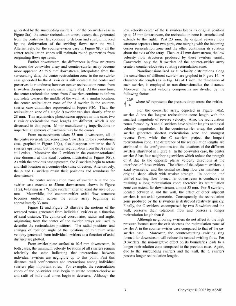
Nondimensionalized axial velocity distributions along the centerlines of different swirlers are graphed in Figure 14. A characteristic length (Ls in Fig. 14) of 1 inch, the dimension of each swirler, is employed to non-dimensionalize the distance. Moreover, the axial velocity components are divided by the following factor:

ρP∆2 where ∆P represents the pressure drop across the swirler.

For the co-swirler array, depicted in Figure 14(a), swirler A has the longest recirculation zone length with the smallest magnitude of reverse velocity. Also, the recirculation zones formed by B and C swirlers have similar lengths and axial velocity magnitudes. In the counter-swirler array, the central swirler generates shortest recirculation zone and strongest reverse flow, while the C swirlers project the longest recirculation zone. The difference of the recirculation lengths are attributed to the configurations and the locations of the different swirlers illustrated in Figure 3. In the co-swirler case, the center swirler A has four neighboring swirlers which reduce the strength of A due to the opposite planar velocity directions at the interfaces of these swirlers. The effect of the adjacent swirlers is axial symmetric, and the central swirling flow can maintain its original shape albeit with weaker strength. In addition, the unified swirling flow formed far downstream is conducive in retaining a long recirculation zone; therefore its recirculation zone can extend far downstream, almost 53 mm. For B swirlers, located between A and the wall, the effect of other adjacent swirlers is not axial symmetric. Consequently, the recirculation zone produced by the B swirlers is destroyed relatively quickly. Finally, the C swirlers, encompassed by two B swirlers and the wall, preserve their rotational flow and possess a longer recirculation length than B.

Although neighboring swirlers do not affect it, the high pressure formed near the exit shortens the recirculation zone of swirler A in the counter-swirler case compared to that of the co-swirler case. Moreover, the counter-rotating swirling ring formed far downstream will reduce the central swirling flow. For B swirlers, the non-negative effect on its boundaries leads to a longer recirculation zone compared to the previous case. Again, due to the surrounding swirlers and the wall, the C swirlers possess longer recirculation lengths.


Mean Swirling velocity

The horizontal velocity distribution is presented in vector form with the x-direction component, denoted “u”, measured directly from the experiment and the y-component, denoted “v”, mathematically derived from the measurements. Although the derived properties may introduce errors near the swirler exit due to discrete jet holes of each swirler, the procedure provides information regarding the swirling flow pattern.

A vector plot of mean horizontal velocities distribution at 3 mm downstream is provided in Figure 15. In both cases, a swirling flow characterizes each swirler, because of the tangential jets relative to each individual swirler axis. However, the swirling flow is not uniform at this axial location; and the discrete air jet flow patterns are easily identified. The peak horizontal velocity is approximately 50 m/s, which is equivalent to the maximum axial mean velocity. Due to the different configurations, the rotation directions are counter-clockwise for all flows in the co-swirler array and alternating between rotational directions for each adjacent swirling flow in the counter-swirler array.

At 13 mm downstream, flow structures between swirlers begin interacting, as shown by the vector plot in Figure 16(a). For the co-swirler case, the original rotating flow structures are destroyed; and a complicated flow structure forms due to the opposing flow directions at the boundaries of neighboring swirlers. This asymmetrical effect leads to the quick deformation of the swirling flows near the wall. Moreover, the swirling flows continuously and gradually merge with each other with increasing axial distance as illustrated in Figure 17(a). Finally, a unified swirling flow zone is formed, and the swirler array behaves like a single swirler.

Alternatively, for the counter-swirler case, the original individual swirling flow maintains its integrity longer than the previous case, until 33 mm, due to similar flow directions at intersects of swirlers. Again, the asymmetrical effect of the wall leads to the deformation of the flow structures induced by the B swirlers. Past 33 mm, the horizontal flow behaves like a counter-rotating swirler. Besides a swirling flow located along the central axis of the array, a counter-rotating swirling ring form around the exterior wall, shown in Figure 16(b), and this flow pattern is retained until 53 mm from the array. Then, the central swirling flow gradually deforms due to the interactions with the counter swirling flow, and four small counter-rotating flows exist within the corner regions illustrated in Figure 17(b). Therefore, the wall preserves the swirling flow and maintains it far downstream.

In both cases, the existence of a global swirling flow structure downstream causes the deformation and spiral motion of individual recirculation zones from the exterior swirlers. To clearly identify the axial locations where the unified swirling flow structure is formed, the angle between horizontal velocity vectors and the radial direction, originated from the center of

swirler array, are calculated. This angle is defined through the

following relationship: RVVR ×=θsin

When the right hand side equals one, the velocity is perpendicular to the radial direction and possesses the same swirling direction as the swirler array. But, when this value equals negative one, the relation indicates a counter-swirling direction. Figure 18 illustrates the distribution of this value in a vertical plane through the origin for the co-swirler (a) and counter-swirler (b) cases.

For the co-swirler case near the swirler plate, counter-rotating areas exist between the array center and the wall, due to the swirling motions generated from individual swirlers. Furthermore, these areas expand up to a distance of 10.5 mm from the array attributable to the expansion of the discrete air jets. Then, the interactions between swirling flows gradually reduce the strength of counter-swirling flows further downstream. At 33 mm downstream, all counter-rotating contours vanish, and the array behaves like a single swirler. For the counter-swirler case, interactions between flow structures occur approximately 10.5 mm from the array, similar to the opposite case. Then, the counter-rotating region diminishes quickly due to these interactions between the swirling flows. Further downstream, the center swirling flow extends to 50 mm leading to the formation of a unified swirling ring.

Turbulent Kinetic Energy

The turbulent kinetic energy is calculated from the LDV

rms measurements and is defined as follows: ( )

2

2_

2_

2_ rmszrmsyrmsx UUU

k++

=

At a location of 3 mm downstream of the array, both cases exhibit three distinct zones of turbulent kinetic energy, depicted in Figure 19. First, high turbulent kinetic energy is distributed along each air jet due to the high velocity gradient between the jet and ambience. The maximum turbulent kinetic energy peaks at 600 m2/s for both cases. Second, low turbulent intensity zones are located within the center recirculation zones above each swirler, where the low mean velocity magnitudes and low velocity gradients contribute to the low turbulence levels. Finally, at the intersections of the swirlers, slightly different phenomena occur between the two cases. In co-swirler case (a), low turbulence intensities exist in these areas, due to the low velocity magnitude and gradient. Alternatively, for the counter-swirler case (b), the strong reverse flows leads to higher turbulence and, thusly, higher turbulent energy.

Further downstream, at 10.5 mm, the rotating flows generated by the array expand to the point of interacting with each other, causing the maximum levels of turbulence intensity distributed along the boundaries between swirlers. In addition, the turbulence intensities of recirculation zones near the wall increase dramatically from the previously considered axial location due to the asymmetrical interactions with the wall and


neighboring swirling flows. One difference exists between the two cases at this location. In the co-swirler case, the center recirculation zone of swirler A possesses the lowest turbulence kinetic energy; but for the other case, the turbulent kinetic energy of the same swirler increases quickly. This relationship is consistent with the shorter length of the recirculation zone for the counter-rotational case.

As the flow moves downstream, in both cases, the turbulence intensity decays rapidly, and the distributions become more uniform across the array, illustrated in Figure 21 at a location of 23 mm downstream and Figure 22 at a location 33 mm downstream for both cases. Also, a distribution of the turbulent kinetic energy distribution within a vertical plane through the y-axis for both configurations, shown in Figure 23, exhibits the decaying nature of turbulent flow at different axial positions. Approximately 10 mm downstream from the array, a highly turbulent structure resides at the boundary of neighbor swirlers Figure 23. Conversely, at an axial location of 33 mm, the localized turbulence distributions combine and begin to uniformly decay to lower levels. Lastly, the increase in turbulence intensity of the center swirler for the counter-rotational case, illustrated in Figure 23(b), is smaller in comparison to the co-rotational case, displayed in Figure 23(a).

CONCLUSIONS

In conclusion, detailed LDV measurements of mean velocity and turbulent energy characteristics of a rotating flow generated by two different swirler array configurations were taken and reported. Also, velocity measurements of a single swirler were interpolated from the data close to the individual swirler exit ports and employed to discuss the flow structures generated by each array arrangement.

The experimental results indicate that the considered flow field has a very complicated structure, especially for the flow structures before 33 mm downstream. In this region, a high turbulent flow structure exists, due to the agitation of the air jets and the interaction between adjacent swirling flows. Past this point, the individual swirler flow structures unify. In comparison, the flow field generated by a co-swirler array deforms rapidly and at an axial distance far from the array behaves similar to the flow generated by a single swirler. Meanwhile, the counter-swirler array retains the individual swirler characteristics across a longer distance due to the amplifying interactions between adjoining swirlers, and the individually generated flow structures unify into a single counter-rotational flow at an axial distance far from the array.

For further research, each array shall be subjected to a combustible environment. Similar flow structure characteristics for each case, such as velocity and turbulence intensities, shall be measured during this experiment, and the data presented in a comparable manner. Furthermore, NOx emissions from this process shall be measured and evaluated between the two cases. Additional conclusions based on this data shall be proposed regarding the applications of these two types of swirler arrays.

REFERENCES 1. Tacina, R., Wey, C., Laing, P., and Mansour, A., “A Low

NOx Lean_Direct Injection, MultiPoint Integrated Module Combustor Concept for Advanced Aircraft Gas Turbines,” NASA Glenn Research Center Technical Report, 2001.

2. Beer J. M., Combustion Aerodynamics, pp. 100-146, 1977. 3. Gupta A. K., Swirl Flows, Academic Press. 1984. 4. Lilley D. G., “Swirl Flows in Combustion: A review,” AIAA

Journal, vol.15, no. 8, pp. 1063-1078. 5. Ahmed S. A., “ Velocity Measurements and Turbulence

Statistics of a Confined Isothermal Swirling Flow,” Experimental thermal and science, vol. 17, pp. 256-264, 1998.

6. Bach, T. Vu, Gouldin, F. C., “Flow measurements in a Model Swirl combustor,” AIAA Journal, vol. 20, pp. 642-651, 1980.

7. Gouldin, F. C., Depsky, J. S., And Lee, S-L, “Velocity Field Characteristics of a Swirling Flow Combustor.” AIAA Journal, vol. 23, pp. 95-102, 1985.

8. Ramos, J. I., and Somer, H. T., “Swirling Flow in a Research Combustor,” AIAA Journal, vol. 23, pp. 241-248, 1985.

9. Halpin, J. L., “Swirl Generation and Recirculation Using Radial Swirl Vanes,” ASME, 93-GT-169.

10. Wang, H., McDonell, V. G., Sowa, W. A., and Samulsen, S. G., “Scaling of the Two-Phase Flow Downstream of a Gas Turbine Combustor Swirl Cup: Part I- Mean Quantities,” Journal of Engineering for Gas Turbines and Power, vol. 115, pp.453-460, 1993.

11. Wang, H., McDonell, V. G., Sowa, W. A., and Samulsen, S. G., “Experimental Study of a Model Gas Turbine Combustor Swirl Cup, Part I: Two-Phase Characterization,” Journal of Propulsion and Power, vol. 10, pp.441-445, 1994.

12. Wang, H., McDonell, V. G., Sowa, W. A., and Samulsen, S., “Experimental Study of a Model Gas Turbine Combustor Swirl Cup, Part II: Droplet Dynamics,” Journal of Propulsion and Power, vol. 10, pp. 446-452, 1994.

13. Cai, J., Jeng, S. M., and Tacina, R., “Multi-Swirler Aerodynamics: Experimental Measurements,” AIAA-2001-3574.

Copyright © 2002 by ASME 6

3mm 5.5mm8mm10.5mm13mm18mm23mm28mm33mm

43mm

53mm

63mm

Air

Air

Cooling air Porous material

Quick &uniformmixing

Completecombustion

Fuel Lean CombustionSmall recirculationzone

MultiPoint Injector/Swirler

Low NOxCombustionProducts

Figure 1. Multi-Point Lean Direct Injection Combustor

Figure 2. Multi-swirler array

Figure 4. Schematic of experimental setup

Figure 5. Measurement locations

Figure 6. Anti-symmetry assumption of horizontal velocity

B2 C

B2 A B1

C B1 C

Figure 3. Measurement area and swirler array types

a. Co-swirler array b. Counter-swirler array

B1

C

C C

B2 A

C B1

B2

U1

V1 V2

U2

X

Y

V1=-U2V2=-U1

Symmetry line

Compressor

Demoisture System

Air Tank

PTP

Orifice Flow Meter

Filter

Pressure Regulator

Particle seeder

P

Temperature output

Pressure output

Multi-swirler

PC

PC LDV Processor

Fiber cable

3W Argon Laser

Receiver Transmitter

3D Travers

Fiber Driver

Fiber Cable

C

Plexglass enclosure


Figure 7. Mean axial velocity contours at 3mm downstream

X (mm)

Y(m

m)

-20 0 20 40

-30

-20

-10

0

10

20

30

454035302520151050

-5-10-15-20-25

Axial mean velocity distribution at 3mm downstream

Uz (m/s)

a. Co-swirler case b. Counter-swirler case

X (mm)

Y(m

m)

-20 0 20 40

-30

-20

-10

0

10

20

30

454035302520151050

-5-10-15-20-25


Uz (m/s)

Figure 8. Mean axial velocity contours at 12mm downstream a. Co-swirler case b. Counter-swirler case

X (mm)

Y(m

m)

-20 0 20 40

-30

-20

-10

0

10

20

30

454035302520151050

-5-10-15-20-25

Axial mean velocity distribution at 25.5mm downstream

Uz (m/s)

Figure 9. Mean axial velocity contour at 25.5mm downstream a. Co-swirler case b. Counter-swirler case

X (mm)

Y(m

m)

-20 0 20 40

-30

-20

-10

0

10

20

30

454035302520151050

-5-10-15-20-25

Axial mean velocity distribution at 3 mm downstream

Uz (m/s)

X (mm)

Y(m

m)

-20 0 20 40

-30

-20

-10

0

10

20

30

454035302520151050

-5-10-15-20-25


Uz (m/s)

X (mm)

Y(m

m)

-20 0 20 40

-30

-20

-10

0

10

20

30454035302520151050

-5-10-15-20-25

Axial mean velocity distribution at 25.5 mm downstream

Uz (m/s)

X (mm)

Y(m

m)

-20 0 20 40

-30

-20

-10

0

10

20

30

454035302520151050

-5-10-15-20-25


Uz (m/s)

X (mm)

Y(m

m)

-20 0 20 40

-30

-20

-10

0

10

20

30

454035302520151050

-5-10-15-20-25


Uz (m/s)

Figure 10. Mean axial velocity contour at 33 mm downstream a. Co-swirler case b. Counter-swirler case


Z/Ls

Uz/

(2P/

ρ)0.

5

0 1 2-0.3

-0.25

-0.2

-0.15

-0.1

-0.05

0

0.05

0.1

0.15

Swirler ASwirler B1Swirler B2Swirler CZero line

Mean Axial velocity distributions along centerlines

Figure 11. Mean axial velocity contour at 53 mm downstream a. Co-swirler case b. Counter-swirler case

X (mm)

Y(m

m)

-20 0 20 40

-30

-20

-10

0

10

20

30454035302520151050

-5-10-15-20-25


Uz (m/s)

X (mm)

Y(m

m)

-20 0 20 40

-30

-20

-10

0

10

20

30

454035302520151050

-5-10-15-20-25


Uz (m/s)

Figure 13. Rotating angle changes of recirculation zones

Fig. 12 Radial changes of recirculation Zones

Z/Ls

Uz/

(2P/

ρ)0.

5

0 0.5 1 1.5 2 2.5-0.3

-0.2

-0.1

0

0.1

Swirler ASwirler B1Swirler B2Swirler Czero line

Mean axial velocity distribution along centerlines

Figure 14. Axial velocity distributions along centerline a. Co-swirler case b. Counter-swirler case

Figure 15. Mean horizontal velocity vectors at 3mm

X (mm)

Y(m

m)

-20 0 20 40

-30

-20

-10

0

10

20

30

Horizontal velocity vector distribution at 3mm downstream

Ref. 50m/s

a. Co-swirler case b. Counter-swirler case X (mm)

Y(m

m)

-20 0 20 40

-30

-20

-10

0

10

20

30

Horizontal velocity vector distribution at 3 mm downstream

Ref. 50m/s

Z (mm)

Ang

le(d

egre

e)

0 10 20 30 40 50 60-10-505

10152025303540455055606570

Swirler B of co-swirler array

Swirler B of counter-swirler array

Swirler C of co-swirler array

Z (mm)

Rad

ius

(mm

)

0 10 20 30 40 50 600

5

10

15

20

25

30

35

40

Swirler B of co-swirler array

Swirler B of counter-swirler array

Swirler C of co-swirler array



X (mm)

Y(m

m)

-20 0 20 40

-30

-20

-10

0

10

20

30


Ref. 10m/s


Y(m

m)

-20 0 20 40

-30

-20

-10

0

10

20

30

Horizontal velocity distribution at 63 mm downstream

Ref.(10m/s)

X (mm)

Z(m

m)

-20 0 20

10

20

30

40

50

60

70

10.90.80.70.60.50.40.30.20.10

-0.1-0.2-0.3-0.4-0.5-0.6-0.7-0.8-0.9-1

Horizontal velocity vector angle distributionalong a vertical plane(Y=0)

Sinθ

Figure 18. Horizontal velocity vector angles distribution at the vertical plane (Y=0) a. Co-swirler case b. Counter-swirler case

X (mm)

Y(m

m)

-20 0 20

10

20

30

40

50

60

70

10.90.80.70.60.50.40.30.20.10

-0.1-0.2-0.3-0.4-0.5-0.6-0.7-0.8-0.9-1

Horizontal velocity vector angle distributionalong a vertical plane (Y=0)

Sinθ

Figure 19. Turbulent kinetic energy distribution at 3mm downstream a. Co-swirler case b. Counter-swirler case

x

y

-20 0 20 40

-30

-20

-10

0

10

20

30

38036034032030028026024022020018016014012010080604020

Turbulent kinetic energy distribution at 3 mm downstream

k (m2/s)

X (mm)

Y(m

m)

-20 0 20 40

-30

-20

-10

0

10

20

3038036034032030028026024022020018016014012010080604020


k (m2/s)


X (mm)

Y(m

m)

-20 0 20 40

-30

-20

-10

0

10

20

30


Ref. 15m/s


Y(m

m)

-20 0 20 40

-30

-20

-10

0

10

20

30

Horizontal velocity vector distribution at 13 mm downstream

Ref.(15m/s)



x

y

-20 0 20 40

-30

-20

-10

0

10

20

30

38036034032030028026024022020018016014012010080604020


k (m2/s)

X (mm)

Y(m

m)

-20 0 20 40

-30

-20

-10

0

10

20

30

38036034032030028026024022020018016014012010080604020


k (m2/s)


x

y

-20 0 20 40

-30

-20

-10

0

10

20

30

38036034032030028026024022020018016014012010080604020


k (m2/s)

X (mm)

Y(m

m)

-20 0 20 40

-30

-20

-10

0

10

20

3038036034032030028026024022020018016014012010080604020


k (m2/s)

Figure 23. Turbulent kinetic energy distribution at a vertical plane a. Co-swirler case b. Counter-swirler case

x

z

-20 0 20

10

20

30

40

50

60

70

38036034032030028026024022020018016014012010080604020

Turbulent kinetic energy distribution at a vertical plane (Y=0)

K(m2/s)

X (mm)

Y(m

m)

-20 0 20

10

20

30

40

50

60

70

38036034032030028026024022020018016014012010080604020

Turbulent kinetic energy distribution at a vertical plane (Y=0)

k (m2/s)

Figure 20. Turbulent kinetic energy distribution at 10.5mm downstream a. Co-swirler case b. Counter-swirler case

x

y

-20 0 20 40

-30

-20

-10

0

10

20

30

38036034032030028026024022020018016014012010080604020

Turbulent kinetic energy distribution at 10.5 mm downstream

k (m2/s)

X (mm)

Y(m

m)

-20 0 20 40

-30

-20

-10

0

10

20

3038036034032030028026024022020018016014012010080604020

Turbulent kinetic energy distribution at 10.5 mm downstream

k (m2/s)

MULTI-SWIRLER AERODYNAMICS: COMPARISON OF …

Documents

Transcript of MULTI-SWIRLER AERODYNAMICS: COMPARISON OF …