Strain calculations for structured semiconductors Diplomarbeit

Multi-Strain Age-Structured DengueTransmission Model: Analysis and
Optimal Control ∗
Michelle N. Raza1 and Randy L. Caga-anan2
Department of Mathematics and StatisticsCollege of Science and MathematicsMSU-Iligan Institute of Technology
Tibanga, Iligan [email protected]
Abstract
Dengue is a serious health problem in the Philippines. In 2016, theDepartment of Health of the country launched a dengue vaccinationcampaign using Dengvaxia. However, the campaign was mired withcontroversy and the use of Dengvaxia was banned in the country. Thisstudy proposes a mathematical model that represents the dynamics ofthe transmission of dengue with its four strains. Considering that theDengvaxia vaccine was intended to be given only to people aging from9 to 45 years old, the human population is divided into two age groups:from 9-45 years old and the rest of the population. Using this modeland optimal control theory we simulate what could have been the effectof Dengvaxia in the number of dengue cases and then compare thiswith the other usual dengue intervention strategies. Results show thatthe best implementation of the usual strategies is better than that ofDengvaxia.
AMS Subject Classification (2010): 92D30, 37N25, 49N90
Keywords: dengue, dengvaxia, SIR, optimal control
∗The first author was funded by the Department of Science and Technology (DOST) ofthe Philippines and the second author by the Premier Research Institute of Science andMathematics (PRISM) of MSU-IIT.
1
arX
iv:1
908.
0219
6v1
[q-
bio.
PE]
6 A
ug 2
019

Multi-Strain Age-Structured Dengue Transmission Model 2
1 Introduction
Dengue is a a mosquito-borne viral infection for which there is no specific anti-viral treatment. Dengue virus is transmitted by female mosquitoes mainlyof the species Aedes aegypti and, to a lesser extent, Aedes albopictus. Thereare four dengue virus serotypes, namely DEN-1, DEN-2, DEN-3, and DEN-4.Infection by one serotype confers life-long immunity to that serotype, but thereis no cross-protective immunity to the other serotypes.
An effective technique used to detect dengue virus and the specific serotypehas been developed. This laboratory test involves taking clinical samples andanalyzing it through the use of Polymerase Chain Reaction (PCR) [9]. Thoughthe method is very efficient, the laboratory test costs from 4,500 to 7,000 pesoswhich is expensive for an average Filipino [2]. Data shows that there were atotal of 69,088 of dengue cases reported nationwide from January 1 to July 28,2018 but only 301 cases were confirmed via PCR [8].
According to the World health Organization, 40 percent of the global pop-ulation is estimated to be at risk of dengue fever [29]. Hence, there is a growingpublic health need for effective preventive interventions against dengue. Deng-vaxia is the first dengue vaccine to be licensed. The vaccine was intended toprevent all four dengue types in individuals from 9 to 45 years of age livingin endemic areas. In 2017, the manufacturer recommended that the vaccineonly be used in people who have previously had a dengue infection, as out-comes may be worsened in those who have not been previously infected.Thishas caused a scandal in the Philippines where more than 733,000 childrenwere vaccinated regardless of serostatus [30]. News have exposed deaths dueto Dengvaxia and because of this the use of the vaccine is now permanentlybanned in the country.
In this paper, we propose a compartmental model describing the dynam-ics of dengue transmission considering its four strains. The model is age-structured taking into account the age requirement for the implementation ofthe Dengvaxia vaccine. Structuring our model this way helps us easily incorpo-rate the control variable for Dengvaxia. There are existing models consideringthe four strains of dengue but our proposed model have the advantage of fo-cusing only on the number of strains a person have been infected to and donot need any information on what specific strain(s) the person have been in-fected to. This is mathematically advantageous because the model now needsfewer equations than when one needs to be specific about the strains. Thisstudy aims to know how effective Dengvaxia could have been if it was imple-mented succesfully. This could be done by using optimal control theory on ourmodel. Since Dengvaxia is now banned in the country, we also investigate onthe other usual alternatives, like vector control and seeking early medical helpand compare these with Dengvaxia.
Multi-Strain Age-Structured Dengue Transmission Model 3
2 Model Formulation
The proposed model considers eight susceptible classes depending on how manytimes a person was infected with dengue. The researcher considers primary,secondary, tertiary and quaternary infection considering the four serotypes ofdengue. But unlike the model in [1], the specific kind of strain that infectsthe person will not matter anymore. The model divides the human populationinto two compartments: 9-45 years old human population and the rest ofthe human population taking into account the age implemetantation of theDengvaxia vaccine. Pandey et al. [25] compared SIR model and vector-hostmodel in dengue transmission and finds it that explicitly incorporating themosquito population may not be necessary in modeling dengue transmissionfor some populations.
The total population at time t, denoted by N(t), is subdivided into eighteencompartments. Age group a consist of individuals of age less than 9 years orgreater than 45 years. Age group b consist of individuals of age 9 up to 45years. Let i = 1, 2, 3, 4 and j = a, b. We denote by Sij(t) the number ofindividuals of age group j who are susceptible to i strain(s) at time t; Iij(t)the number of individuals of age group j who were infected with any i − 1strain(s) in the past and is currently (at time t) infected with a different strain;and Rj is the number of individuals of age group j who had been infected byall the strains and has now (at time t) completely recovered. It is assumedthat all individuals are born susceptible to any of the dengue strains and thusenter the class S4a and a recovered individual from a strain of dengue willhave complete immunity to that strain. Humans leave the population throughnatural death rate and through per-capita death rate due to infection. Humansof age less than 9 years in the susceptible class (Sia) leave the population andmove to infected class (Iia) or grow older to susceptible class Sib. Furthermore,humans of age greater than 45 years in the susceptible class (Sib) leave thepopulation and move to infected class (Iib) or grow older to susceptible classSia. In general, any member of the human population remains susceptiblewith the four strains of dengue and stays in the class S4j for a certain periodunless bitten and infected with one strain. Once in the infective class I1j,an individual may die or recover from that strain. If recovered from the firstinfection, susceptibility remains to the other 3 strains and then transfered toS3j. If the same individual is infected with another strain, then he will bemoved to the class I2j. Once recovered from that strain, he is still susceptibleto the other two strains and now belongs to the class S2j. The cycle repeatsuntil the individual gets infected four times and identified into the class I4j. Ifever the person survived the fourth infection, he then completely recovers andremains in the class Rj.
The parameters used are transmission coefficient (αij), recovery rate (βij),

Multi-Strain Age-Structured Dengue Transmission Model 4
birth rate (µ), natural death rate (δ), per-capita death rate through infection(γij), rate of progression from age group a to b (εa), and rate of progressionfrom age group b to a (εb). The following figure gives the flow diagram of thedengue transmission model.
Figure 1: Flow chart of the model
The model can be mathematically described by the following system of 18

Multi-Strain Age-Structured Dengue Transmission Model 5
differential equations:
dS4a
dt= µN + εbS4b − (εa + δ)S4a −
α1aS4aI
NdSiadt
= εbSib + β(4−i)aI(4−i)a − (εa + δ)Sia −α(5−i)aSiaI
N, for i = 1, 2, 3
dIiadt
=αiaS(5−i)aI
N+ εbIib − (εa + δ + γia + βia)Iia, for i = 1, 2, 3, 4
dRa
dt= β4aI4a + εbRb − (δ + εa)Ra (1)
dS4b
dt= εaS4a − (εb + δ)S4b −
α1bS4bI
NdSibdt
= εaSia + β(4−i)bI(4−i)b − (εb + δ)Sib −α(5−i)bSibI
N, for i = 1, 2, 3
dIibdt
=αibS(5−i)bI
N+ εaIia − (εb + δ + γib + βib)Iib, for i = 1, 2, 3, 4
dRb
dt= β4bI4b + εaRa − (εb + δ)Rb
where I =4∑i=1
(Iia + Iib) and N =4∑i=1
(Sia + Sib + Iia + Iib) + Ra + Rb. Note
thatdN
dt= µN − δN −
4∑i=1
(γiaIia + γibIib). To analyze the model, fractional
quantities will be used and this could be done by scaling the population ofeach class with the total population. The new variables will be as follows:
SiA =SiaN, IiA =
IiaN,SiB =
SibN, IiB =
IibN,RA =
Ra
N, and RB =
Rb
N,
for i = 1, 2, 3, 4. Note that capital letters are used as subscripts to denote thescaled quantities. Furthermore, observe that
4∑1
(SiA + SiB + IiA + IiB) +RA +RB = 1
or
S4A = 1−
(3∑i=1
(SiA) +4∑i=1
(SiB + IiA + IiB) +RA +RB
).
Using this and differentiating each fractional quantities with respect to time,
Multi-Strain Age-Structured Dengue Transmission Model 6
the system (1) is reduced to the following system of 17 differential equations:
dI1Adt
= α1aINx+ εbI1B − (εa + µ+ γ1a + β1a)I1A + I1AJ
dSiA
dt= εbSiB + β(4−i)aI(4−i)A − (εa + µ)SiA − α(5−i)aSiAIN + SiAJ, for i = 1, 2, 3
dIiAdt
= αiaS(5−i)AIN + εbIiB − (εa + µ+ γia + βia)IiA + IiAJ, , for i = 2, 3, 4
dRA
dt= β4aI4A + εbRB − (εa + µ)RA +RAJ
dS4B
dt= εax− (εb + µ)S4B − α1bS4BIN + S4BJ (2)
dIiBdt
= α1bS(5−i)BIN + εaIiA − (εb + µ+ γib + βib)IiB + IiBJ, for i = 1, 2, 3, 4
dSiB
dt= εaSiA + β(4−i)bI(4−i)B − (εb + µ)SiB − α(5−i)bSiBIN + SiBJ, for i = 1, 2, 3
dRB
dt= β4BI4B + εaRA − (εb + µ)RB +RBJ
where IN =4∑i=1
(IiA + IiB) and J =∑4
i=1(γiaIiA + γibIiB).
This system of equations is epidemiologically and mathematically well-posed on the domain
D =
(S3A, S2A, S1A, I1A, I2A, I3A, I4A, RA, S4B, S3B, S2B, S1B, I1B, I2B, I3B,
I4B, RB) ∈ R17+
∣∣∣∣ SiA ≥ 0, Iia ≥ 0, RA ≥ 0, SiA ≥ 0, IiA ≥ 0,
RB ≥ 0, where i = 1, 2, 3, 4 and(3∑i=1
(SiA + SiB) + S4B +4∑i=1
(IiA + IiB) +Ra +Rb
)≤ 1
.
The space R17+ denotes the positive orthant in R17.
2.1 Model Analysis
In this section, we obtain the disease-free equilibrium point and the repro-ductive number of the model. A disease-free equilibrium (DFE) is a steadystate solution of an epidemic model with all infected variables equal to zero[6]. Over time, we want to achieve a disease-free state. A threshold that de-termines whether a disease-free state is achievable or not is the reproductivenumber R0. The reproductive number is the expected number of individu-als infected by a single infected individual over the duration of the infectiousperiod in a population, which is entirely susceptible [11]. The reproductionnumber also gives an idea of which parameters in our model may be significant

Multi-Strain Age-Structured Dengue Transmission Model 7
in our dynamics. The next generation operator approach defined by Diekmannet al. [12] and Driessche and Watmough [11] will be used to compute R0.
Theorem 2.1 Assuming that the initial conditions lie in D, the system ofequations (4) has a unique solution that exists and remains in D for all timet ≥ 0.
Proof : Note that the right-hand side of the system of equations (2) is con-tinuous with continuous partial derivatives in D, by Cauchy-Lipschitz The-orem, the system of equations (2) has a unique solution. To show that D
is forward invariant, note that if IiA = 0 thendIiAdt≥ 0 for i = 1, 2, 3, 4.
If SiA = 0 thendSiAdt≥ 0 for i = 1, 2, 3. If SiB = 0 then
dSiBdt
≥ 0 for
i = 1, 2, 3, 4. If IiB = 0 thendIiBdt≥ 0 for i = 1, 2, 3, 4. Note also that if
3∑i=1
(SiA + SiB) + S4B +4∑i=1
(IiA + IiB) +RA +RB = 1, it follows that
3∑i=1
dSiAdt
+4∑i=1
dIiAdt
+4∑i=1
dSiBdt
+4∑i=1
dIiBdt
+dRA
dt+dRB
dt< 0.
Hence, none of the orbits can leave D and a unique solution exists for all time.
Theorem 2.2 The disease-free equilibrium point of the epidemic model (2) is(0, 0, 0, 0, 0, 0, 0, 0,
εaεa + εb + µ
, 0, 0, 0, 0, 0, 0, 0, 0
).
Proof : Set the right-hand side of system (2) to zero and let IiA = IiB = 0 fori = 1, 2, 3, 4. Since µ > 0 and the DFE point is in D, we have S3B = S3A =S2B = S2A = S1B = S1A = RA = RB = 0. With these values, we are left with
ε1(1− S4B)− (ε2 + µ)S4B = 0. Thus, we have S4B =ε1
ε1 + ε2 + µ.
Theorem 2.3 The reproductive number for system (2) is
R0 = α1a
(ε2 + µ
ε1 + ε2 + µ
)((ε2 + µ+ γ1b + β1b + ε1)
(ε1 + µ+ γ1a + β1a)(ε2 + µ+ γ1b + β1b)− ε1ε2
)+ α1b
(ε1
ε1 + ε2 + µ
)((ε1 + µ+ γ1a + β1a + ε2)
(ε1 + µ+ γ1a + β1a)(ε2 + µ+ γ1b + β1b)− ε1ε2
),
and the system is asymptotically stable if R0 < 1 and unstable if R0 > 1.

Multi-Strain Age-Structured Dengue Transmission Model 8
Proof : We form the matrices F and V where F is the matrix of the rates ofappearance of new infections and V is the matrix of the rates of transfer ofindividuals out of the compartments. Let X be the vector of infected classesand Y be the vector of susceptible and recoverd classes.
Let F(X, Y ) be the vector of new infection rates (flows from Y to X).Let V(X, Y ) be the vector of all other rates (not new infection). These ratesinclude flows from X to Y (for instance, recovery rates), flows within X andflows leaving from the system (for instance, death rates). The next generation
operator formed is K = FV −1 where F =
[∂F∂X
], V =
[∂V∂X
]. Evaluated
at the disease-free equilibrium (0, 0, 0, 0, 0, 0, 0, 0, S∗4B, 0, 0, 0, 0, 0, 0, 0, 0) where
S∗4B =εa
εa + εb + µ, this becomes
F (I1A, I2A, . . . , I4B) =
α1ax α1ax α1ax α1ax α1ax α1ax α1ax α1ax0 0 0 0 0 0 0 00 0 0 0 0 0 0 00 0 0 0 0 0 0 0
α1bS∗4B α1bS
∗4B α1bS
∗4B α1bS
∗4B α1bS
∗4B α1bS
∗4B α1bS
∗4B α1bS
∗4B
0 0 0 0 0 0 0 00 0 0 0 0 0 0 00 0 0 0 0 0 0 0
where x = 1− εa
εa + εb + µ=
εb + µ
εa + εb + µ. We also have,
V (I1A, I2A, . . . , I4B) =
v′11 0 0 0 −εb 0 0 00 v′22 0 0 0 −εb 0 00 0 v′33 0 0 0 −εb 00 0 0 v′44 0 0 0 −εb−εa 0 0 0 v′55 0 0 0
0 −εa 0 0 0 v′66 0 00 0 −εa 0 0 0 v′77 00 0 0 −εa 0 0 0 v′88
where
v′11 = εa + µ+ γ1a + β1a v′55 = εb + µ+ γ1b + β1b
v′22 = εa + µ+ γ2a + β2a v′66 = εb + µ+ γ2b + β2b
v′33 = εa + µ+ γ3a + β3a v′77 = εb + µ+ γ3b + β3b
v′44 = εa + µ+ γ4a + β4a v′88 = εb + µ+ γ4b + β4b
Multi-Strain Age-Structured Dengue Transmission Model 9
Moreover,
V −1(I1A, I2A, . . . , I4B) =
d1 0 0 0 b1 0 0 00 d2 0 0 0 b2 0 00 0 d3 0 0 0 b3 00 0 0 d4 0 0 0 b4
c1 0 0 0 d5 0 0 00 c2 0 0 0 d6 0 00 0 c3 0 0 0 d7 00 0 0 c4 0 0 0 d8
where d1 =
v′55
v′11v′55 − εaεb
, d2 =v′66
v′22v′66 − εaεb
, d3 =v′77
v′33v′77 − εaεb
, d4 =v′88
v′44v′88 − εaεb
,
d5 =v′11
v′11v′55 − εaεb
, d6 =−v′22
v′22v′66 − εaεb
, d7 =v′33
v′33v′77 − εaεb
, d8 =v′44
v′44v′88 − εaεb
,
c1 =εa
v′11v′55 − εaεb
, c2 =εa
v′22v′66 − εaεb
, c3 =εa
v′33v′77 − εaεb
, c4 =εa
v′44v′88 − εaεb
,
b1 =εb
v′11v′55 − εaεb
, b2 =εb
v′22v′66 − εaεb
, b3 =εb
v′33v′77 − εaεb
, b4 =εb
v′44v′88 − εaεb
.
Now, the next generation matrix K is formed as
K = F (I1A, I2A, . . . , I4B)V −1(I1A, I2A, . . . , I4B).
Using cofactor expansion to get the eigenvalue of K, we have
|K − λI8| = (λ6)
∣∣∣∣[α1a(1− S∗4B)(d1 + c1)− λ α1a(1− S∗4B)(d5 + b1)α1bS
∗4B(d1 + c1) α1bS
∗4B(d5 + b1)− λ
]∣∣∣∣= (λ6)
[−λα1a(1− S∗4B)(d1 + c1)− λα1bS
∗4B(d5 + b1) + λ2
]= (λ7) [−α1ax(d1 + c1)− α1bS
∗4b(d5 + b1) + λ]
Hence we have, λ = α1ax(d1 + c1) +α1bS∗4b(d5 + b1) and λ = 0 of multiplicity 7.
Taking the dominant eigenvalue of matrix K, we get R0 = α1a(1− S∗4B)(d1 +c1) + α1bS
∗4B(d5 + b1). Substituting the values
S∗4B =εa
εa + εb + µ, x =
εb + µ
εa + εb + µ, d1 =
v′55
v′11v′55 − εaεb
, d5 =v′11
v′11v′55 − εaεb
,
b1 =εb
v′11v′55 − εaεb
, c1 =εa
v′11v′55 − εaεb
, v′11 = εa + µ+ γ1a + β1a,
and v′55 = εb + µ+ γ1b + β1b, we finally have
R0 = α1a
(εb + µ
εa + εb + µ
)((εb + µ+ γ1b + β1b + εa)
(εa + µ+ γ1a + β1a)(εb + µ+ γ1b + β1b)− εaεb
)+ α1b
(εa
εa + εb + µ
)((εa + µ+ γ1a + β1a + εb)
(εa + µ+ γ1a + β1a)(εb + µ+ γ1b + β1b)− εaεb
).

Multi-Strain Age-Structured Dengue Transmission Model 10
3 Optimal Control Strategies
To mitigate the spread of dengue in the Philippines, three control interventionstrategies ui(t), i = 1, 2, 3 were identified to be incorporated in our model tosee its best effects in reducing the number of infected individuals at its bestimplementation with the minimum cost. First is the transmission reduc-tion conrol u1(t). This consists of holistic and effective methods in fightingmosquito at every stage of their life cycle, such as searching and eliminatingbreeding grounds, larvicide treatment, using adult mosquito trap, insecticidesand thermal fogging during outbreaks. This also encompasses environmen-tal management and sources reduction, self-protection measures which is juststrengthening the capability of a person to avoid dengue and health educa-tion to provide awareness for their protection against dengue. Next strategy isproper medical care control u2(t). This means an effort for patients to seekearly medication and immediate reporting to the nearest health care facilityas symptoms are observed. With this control, chances of recovery increasesspecially from severe dengue. Last control is the Dengvaxia vaccine u3(t).This controversial Dengvaxia vaccine could have been a major breakthroughfor dengue prevention in the country, but, the Philippines holds a lot of pend-ing issues against its implementation. Moreover, it has been banned and notallowed for marketing in the Philippines. In this paper, we would like to knowwhat could be the best effect of Dengvaxia (number of infected individuals areminimized, while the intervention costs are kept low) if it was properly imple-mented, that is, if it had been given only to susceptible population from 9-45years old and to those who have had previous infection. We also investigate onthe best possible impact of the other intervention strategies to compare it withDengvaxia. This study is influenced by a similar study done for tuberculosisin the Philippines in [17].
The dengue state dynamics incorporating the different controls can now be

Multi-Strain Age-Structured Dengue Transmission Model 11
described as follows:
dS4a
dt= µN + εbS4b − (εa + δ)S4a − (1− u1(t))
α1aS4aI
NdSiadt
= εbSib + (1 + u2(t))β(4−i)aI(4−i)a − (εa + δ)Sia
− (1− u1(t))α(5−i)aSiaI
N, for i = 1, 2, 3
dIiadt
= (1− u1(t))αiaS(5−i)aI
N+ εbIib − (εa + δ + γia)Iia
− (1 + u2(t))βiaIia, for i = 1, 2, 3, 4
dRa
dt= (1 + u2(t))β4aI4a + εbRb − (δ + εa)Ra
dS4b
dt= εaS4a − (εb + δ)S4b − (1− u1(t))
α1bS4bI
N(3)
dSibdt
= εaSia + (1 + u2(t))β(4−i)bI(4−i)b − (εb + δ)Sib
− (1− u1(t))α(5−i)bSibI
N− u3Sib, for i = 1, 2, 3
dIibdt
= (1− u1(t))αibS(5−i)bI
N+ εaIia − (εb + δ + γib)Iib
− (1 + u2(t))βibIib, for i = 1, 2, 3
dRb
dt= (1 + u2(t))β4bI4b + εaRa − (εb + δ)Rb
dN
dt= µN − δN −
4∑i=1
(γiaIia + γibIib)− u3(S3b + S2b + S1b)
Transmission reduction control u1(t) is applied on all compartments havingthe transmission rates and proper medical control u2(t) is incorporated on allcompartments involving recovery rates. The Dengvaxia control u3(t) is onlyapplied on age group b since it has restrictions on its implementation to peopleof age 9-45. Moreover, it is not incorporated to the compartment S4b since itmust only be applied to people who have had previous infection.
The controls range is the interval (0, 1). The case when ui(t) ≡ 0 means nocontrol effort is employed while the case ui(t) ≡ 1 indicates maximum admin-istration of the control intervention. In this study, the optimal control problemaims to minimize the number of infected individuals with the minimum imple-mentation cost of the control measure(s). It is assumed that the controls arequadratic functions to incorporate nonlinear societal cost associated with theimplementation of control measures. This quadratic control is a common formof an objective functional in an optimal control problem. If three controls areconsidered u1(t), u2(t) and u3(t), the objective functional to be minimized is

Multi-Strain Age-Structured Dengue Transmission Model 12
represented by
J(u1, u2, u3) =
∫ T1
T0
[I(t) +
B1
2u2
1(t) +B2
2u2
2(t) +B3
2u2
3(t)
]dt
where I(t) =4∑i=1
(Iia(t) + Iib(t)). The bounds T0 and T1 are taken as 2020
and 2040, respectively, to consider a 20-year dengue intervention program andBi’s, i = 1, 2, 3, represent the weight constants associated to the relative costsof implementating the respective control strategy. These constants balancedthe size and importance of each term in the integrand. In this work, we seekto find optimal controls u∗1, u
∗2 and u∗3 satisfying
J(u∗1, u∗2, u∗3) = min
ΩJ(u1, u2, u3),
where Ω =
(u1, u2, u3)∣∣ a ≤ ui(t) ≤ b, ui ∈ L2(2020, 2040), i = 1, 2, 3
. Pa-
rameters a and b are the upper and lower bounds of the controls and areassumed to be 0.05 and 0.95, respectively. The weight parameters are set asB1 = B2 = B3 = 106.
3.1 Main Theorem
The goal is to minimize the number of infected individuals and correspondingcosts. From Pontryagin’s Maximum principle, optimal controls should satisfythe necessary conditions. Pontryagin’s Maximum Principle changes into aproblem that minimize pointwise a Hamiltonian H, with respect to the control.
We have H = I(t) +B1
2u2
1(t) +B2
2u2
2(t) +B3
2u2
3(t) +19∑i=1
λigi, where gi is the
right hand side of the differential equation of the ith state variable. ApplyingPontryagin’s Maximum Principle, we obtain the following theorem.
Theorem 3.1 There exist optimal controls u∗1(t), u∗2(t) and u∗3(t) minimizingthe objective functional
Ω =
(u1, u2, u3)∣∣ a ≤ ui(t) ≤ b, ui ∈ L2(2020, 2040), i = 1, 2, 3
.
Given these optimal solutions, there exist adjoint variables, λ1(t), λ2(t), . . . , λ19(t),which satisfy
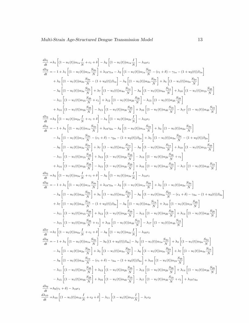
Multi-Strain Age-Structured Dengue Transmission Model 13
dλ1
dt=λ1
[(1− u1(t))α1a
I
N+ ε1 + δ
]− λ2
[(1− u1(t))α1a
I
N
]− λ10ε1
dλ2
dt=− 1 + λ1
[(1− u1(t))α1a
S4a
N
]+ λ19γ1a − λ2
[(1− u1(t))α1a
S4a
N− (ε1 + δ)− γ1a − (1 + u2(t))β1a
]+ λ3
[(1− u1(t))α2a
S3a
N− (1 + u2(t))β1a
]− λ4
[(1− u1(t))α2a
S3a
N
]+ λ5
[(1− u1(t))α3a
S2a
N
]− λ6
[(1− u1(t))α3a
S2a
N
]+ λ7
[(1− u1(t))α4a
S1a
N
]− λ8
[(1− u1(t))α4a
S1a
N
]+ λ10
[(1− u1(t))α1b
S4b
N
]− λ11
[(1− u1(t))α1b
S4b
N+ ε1
]+ λ12
[(1− u1(t))α2b
S3b
N
]− λ13
[(1− u1(t))α2b
S3b
N
]+ λ14
[(1− u1(t))α3b
S2b
N
]− λ15
[(1− u1(t))α3b
S2b
N
]+ λ16
[(1− u1(t))α4b
S1b
N
]− λ17
[(1− u1(t))α4b
S1b
N
]dλ3
dt=λ3
[(1− u1(t))α2a
I
N+ ε1 + δ
]− λ4
[(1− u1(t))α2a
I
N
]− λ12ε1
dλ4
dt=− 1 + λ1
[(1− u1(t))α1a
S4a
N
]+ λ19γ2a − λ2
[(1− u1(t))α1a
S4a
N
]+ λ3
[(1− u1(t))α2a
S3a
N
]− λ4
[(1− u1(t))α1a
S3a
N− (ε1 + δ)− γ2a − (1 + u2(t))β2a
]+ λ5
[(1− u1(t))α3a
S2a
N− (1 + u2(t))β2a
]− λ6
[(1− u1(t))α3a
S2a
N
]+ λ7
[(1− u1(t))α4a
S1a
N
]− λ8
[(1− u1(t))α4a
S1a
N
]+ λ10
[(1− u1(t))α1b
S4b
N
]− λ11
[(1− u1(t))α1b
S4b
N
]+ λ12
[(1− u1(t))α2b
S3b
N
]− λ13
[(1− u1(t))α2b
S3b
N+ ε1
]+ λ14
[(1− u1(t))α3b
S2b
N
]− λ15
[(1− u1(t))α3b
S2b
N
]+ λ16
[(1− u1(t))α4b
S1b
N
]− λ17
[(1− u1(t))α4b
S1b
N
]dλ5
dt=λ5
[(1− u1(t))α3a
I
N+ ε1 + δ
]− λ6
[(1− u1(t))α3a
I
N
]− λ14ε1
dλ6
dt=− 1 + λ1
[(1− u1(t))α1a
S4a
N
]+ λ19γ3a − λ2
[(1− u1(t))α1a
S4a
N
]+ λ3
[(1− u1(t))α2a
S3a
N
]− λ4
[(1− u1(t))α2a
S3a
N
]+ λ5
[(1− u1(t))α3a
S2a
N
]− λ6
[(1− u1(t))α3a
S2a
N− (ε1 + δ)− γ3a − (1 + u2(t))β3a
]+ λ7
[(1− u1(t))α4a
S1a
N− (1 + u2(t))β3a
]− λ8
[(1− u1(t))α4a
S1a
N
]+ λ10
[(1− u1(t))α1b
S4b
N
]− λ11
[(1− u1(t))α1b
S4b
N
]+ λ12
[(1− u1(t))α2b
S3b
N
]− λ13
[(1− u1(t))α2b
S3b
N
]+ λ14
[(1− u1(t))α3b
S2b
N
]− λ15
[(1− u1(t))α3b
S2b
N+ ε1
]+ λ16
[(1− u1(t))α4b
S1b
N
]− λ17
[(1− u1(t))α4b
S1b
N
]dλ7
dt=λ7
[(1− u1(t))α4a
I
N+ ε1 + δ
]− λ8
[(1− u1(t))α4a
I
N
]− λ16ε1
dλ8
dt=− 1 + λ1
[(1− u1(t))α1a
S4a
N
]− λ9 [(1 + u2(t))β4a]− λ2
[(1− u1(t))α1a
S4a
N
]+ λ3
[(1− u1(t))α2a
S3a
N
]− λ4
[(1− u1(t))α2a
S3a
N
]+ λ5
[(1− u1(t))α3a
S2a
N
]− λ6
[(1− u1(t))α3a
S2a
N
]+ λ7
[(1− u1(t))α4a
S1a
N
]− λ8
[(1− u1(t))α4a
S1a
N− (ε1 + δ)− γ4a − (1 + u2(t))β4a
]+ λ10
[(1− u1(t))α1b
S4b
N
]− λ11
[(1− u1(t))α1b
S4b
N
]+ λ12
[(1− u1(t))α2b
S3b
N
]− λ13
[(1− u1(t))α2b
S3b
N
]+ λ14
[(1− u1(t))α3b
S2b
N
]− λ15
[(1− u1(t))α3b
S2b
N
]+ λ16
[(1− u1(t))α4b
S1b
N
]− λ17
[(1− u1(t))α4b
S1b
N+ ε1
]+ λ19γ4a
dλ9
dt=λ9(ε1 + δ)− λ18ε1
dλ10
dt=λ10
[(1− u1(t))α1b
I
N+ ε2 + δ
]− λ11
[(1− u1(t))α1b
I
N
]− λ1ε2

Multi-Strain Age-Structured Dengue Transmission Model 14
dλ11
dt=− 1 + λ1
[(1− u1(t))α1a
S4a
N
]− λ2
[(1− u1(t))α1a
S4a
N+ ε2
]+ λ3
[(1− u1(t))α2a
S3a
N
]− λ4
[(1− u1(t))α2a
S3a
N
]+ λ5
[(1− u1(t))α3a
S2a
N
]− λ6
[(1− u1(t))α3a
S2a
N
]+ λ7
[(1− u1(t))α4a
S1a
N
]− λ8
[(1− u1(t))α4a
S1a
N
]+ λ10
[(1− u1(t))α1b
S4b
N
]− λ11
[(1− u1(t))α1b
S4b
N− (ε2 + δ)− γ1b − (1 + u2(t))β1b
]+ λ12
[(1− u1(t))α2b
S3b
N− (1 + u2(t))β1b
]− λ13
[(1− u1(t))α2b
S3b
N
]+ λ14
[(1− u1(t))α3b
S2b
N
]− λ15
[(1− u1(t))α3b
S2b
N
]+ λ16
[(1− u1(t))α4b
S1b
N
]− λ17
[(1− u1(t))α4b
S1b
N
]+ λ19γ1b
dλ12
dt=λ12
[(1− u1(t))α2b
I
N+ ε2 + δ + u3
]− λ13
[(1− u1(t))α2b
I
N
]− λ3ε2 + λ19u3
dλ13
dt=− 1 + λ1
[(1− u1(t))α1a
S4a
N
]− λ2
[(1− u1(t))α1a
S4a
N
]+ λ3
[(1− u1(t))α2a
S3a
N
]− λ4
[(1− u1(t))α2a
S3a
N+ ε2
]+ λ5
[(1− u1(t))α3a
S2a
N
]− λ6
[(1− u1(t))α3a
S2a
N
]+ λ7
[(1− u1(t))α4a
S1a
N
]− λ8
[(1− u1(t))α4a
S1a
N
]+ λ10
[(1− u1(t))α1b
S4b
N
]− λ11
[(1− u1(t))α1b
S4b
N
]+ λ12
[(1− u1(t))α2b
S3b
N
]− λ13
[(1− u1(t))α2b
S3b
N− (ε2 + δ)− γ2b − (1 + u2(t))β2b
]+ λ19γ2b
+ λ14
[(1− u1(t))α3b
S2b
N− (1 + u2(t))β2b
]− λ15
[(1− u1(t))α3b
S2b
N
]+ λ16
[(1− u1(t))α4b
S1b
N
]− λ17
[(1− u1(t))α4b
S1b
N
]dλ14
dt=λ14
[(1− u1(t))α3b
I
N+ ε2 + δ + u3
]− λ15
[(1− u1(t))α3b
I
N
]− λ5ε2 + λ19u3
dλ15
dt=− 1 + λ1
[(1− u1(t))α1a
S4a
N
]− λ2
[(1− u1(t))α1a
S4a
N
]+ λ3
[(1− u1(t))α2a
S3a
N
]− λ4
[(1− u1(t))α2a
S3a
N
]+ λ5
[(1− u1(t))α3a
S2a
N
]− λ6
[(1− u1(t))α3a
S2a
N+ ε2
]+ λ7
[(1− u1(t))α4a
S1a
N
]− λ8
[(1− u1(t))α4a
S1a
N
]+ λ10
[(1− u1(t))α1b
S4b
N
]− λ11
[(1− u1(t))α1b
S4b
N
]+ λ12
[(1− u1(t))α2b
S3b
N
]− λ13
[(1− u1(t))α2b
S3b
N
]− λ15
[(1− u1(t))α3b
S2b
N− (ε2 + δ)− γ3b − (1 + u2(t))β3b
]+ λ14
[(1− u1(t))α3b
S2b
N
]+ λ16
[(1− u1(t))α4b
S1b
N− (1 + u2(t))β3b
]− λ17
[(1− u1(t))α4b
S1b
N
]+ λ19γ3b
dλ16
dt=λ16
[(1− u1(t))α4b
I
N+ ε2 + δ + u3
]− λ17
[(1− u1(t))α4a
I
N
]− λ7ε2 + λ19u3
dλ17
dt=− 1 + λ1
[(1− u1(t))α1a
S4a
N
]− λ18 [(1 + u2(t))β4b]− λ2
[(1− u1(t))α1a
S4a
N
]+ λ3
[(1− u1(t))α2a
S3a
N
]− λ4
[(1− u1(t))α2a
S3a
N
]+ λ5
[(1− u1(t))α3a
S2a
N
]− λ6
[(1− u1(t))α3a
S2a
N
]+ λ7
[(1− u1(t))α4a
S1a
N
]− λ8
[(1− u1(t))α4a
S1a
N+ ε2
]+ λ10
[(1− u1(t))α1b
S4b
N
]− λ11
[(1− u1(t))α1b
S4b
N
]+ λ12
[(1− u1(t))α2b
S3b
N
]− λ13
[(1− u1(t))α2b
S3b
N
]+ λ14
[(1− u1(t))α3b
S2b
N
]− λ15
[(1− u1(t))α3b
S2b
N
]+ λ18 [(1 + u2(t))β4b]
+ λ16
[(1− u1(t))α4b
S1b
N
]− λ17
[(1− u1(t))α4b
S1b
N− (ε2 + δ)− γ4b − (1 + u2(t))β4b
]+ λ19γ4b
dλ18
dt=λ18(ε2 + δ)− λ9ε2

Multi-Strain Age-Structured Dengue Transmission Model 15
dλ19
dt=− λ1
[µ+ (1− u1(t))α1a
S4aI
N2
]+ λ2
[(1− u1(t))α1a
S4aI
N2
]− λ3
[(1− u1(t))α2a
S3aI
N2
]+ λ4
[(1− u1(t))α2a
S3aI
N2
]− λ5
[(1− u1(t))α3a
S2aI
N2
]+ λ6
[(1− u1(t))α3a
S2aI
N2
]− λ7
[(1− u1(t))α4a
S1aI
N2
]+ λ8
[(1− u1(t))α4a
S1aI
N2
]− λ10
[(1− u1(t))α1b
S4bI
N2
]+ λ11
[(1− u1(t))α1b
S4bI
N2
]− λ12
[(1− u1(t))α2b
S3bI
N2
]+ λ13
[(1− u1(t))α2b
S3bI
N2
]+ λ19 [µ− δ]
− λ14[(1− u1(t))α3b
S2bI
N2
]+ λ15
[(1− u1(t))α3b
S2bI
N2
]− λ16
[(1− u1(t))α4b
S1bI
N2
]+ λ17
[(1− u1(t))α4b
S1bI
N2
]
with transversality conditions λi(tf ) = 0, for i = 1, 2, . . . , 19. Furthermore,
u∗1(t) = min
(b,max
(a,−ZB1
)),
u∗2(t) = min
(b,max
(a,−XB2
)),
u∗3(t) = min
(b,max
(a,λ12S3b + λ14S2b + λ16S1b + λ19 [S3b + S2b + S1b]
B3
))where
Z = λ1α1aS4aI
N− λ2
(α1aS4aI
N
)+ λ3
α2aS3aI
N− λ4
(α2aS3aI
N
)λ5α3aS2aI
N− λ6
(α3a
S2aI
N
)+ λ7
α4aS1aI
N− λ8
(α4aS1aI
N
)λ10
α1bS4bI
N− λ11
(α1bS4bI
N
)+ λ12
α2bS3bI
N− λ13
(α2b
S3bI
N
)λ14
α3bS2bI
N− λ15
(α3b
S2bI
N
)+ λ16
α4bS1bI
N− λ17
(α4bS1bI
N
)and
X = (λ3 − λ2)β1aI1a + (λ5 − λ4)β2aI2a + (λ7 − λ6)β3aI3a
(λ9 − λ8)β4aI4a + (λ12 − λ11)β1bI1b + (λ14 − λ13)β2bI2b
+ (λ16 − λ15)β3bI3b + (λ18 − λ17)β4bI4b.
Proof : The existence of optimal controls u∗1(t), u∗2(t), and u∗3(t) such thatJ(u∗1(t), u∗2(t), u∗3(t)) = min
Ω(u1, u2, u3), with state system (3) is given by the
convexity of the objective functional integrand. By Pontryagin’s MaximumPrinciple, the adjoint equations and transversality conditions can be obtained.Differentiation of the Hamiltonian H with respect to the state variable givesthe following system:dλ1
dt= − ∂H
∂S4a
,dλ2
dt= − ∂H
∂I1a
,dλ3
dt= − ∂H
∂S3a
,dλ4
dt= − ∂H
∂I2a
,
dλ5
dt= − ∂H
∂S2a
,dλ6
dt= − ∂H
∂I3a
,dλ7
dt= − ∂H
∂S1a
,dλ8
dt= − ∂H
∂I4a
,
dλ9
dt= − ∂H
∂Ra
,dλ10
dt= − ∂H
∂S4b
,dλ11
dt= − ∂H
∂I1b
,dλ12
dt= − ∂H
∂S3b
,

Multi-Strain Age-Structured Dengue Transmission Model 16
dλ13
dt= − ∂H
∂I2b
,dλ14
dt= − ∂H
∂S2b
,dλ15
dt= − ∂H
∂I3b
,dλ16
dt= − ∂H
∂S1b
,
dλ17
dt= − ∂H
∂I4b
,dλ18
dt= − ∂H
∂Rb
,dλ19
dt= −∂H
∂N,
with λi(tf ) = 0, for i = 1, 2, . . . , 19.Optimal controls u∗1(t), u∗2(t), and u∗3(t) are derived by the following opti-
mality conditions:
∂H
∂u1=B1u1 +
[λ1α1aS4aI
N− λ2
(α1aS4aI
N
)+ λ3
α2aS3aI
N− λ17
(α4bS1bI
N
)− λ4
(α2aS3aI
N
)+ λ5
α3aS2aI
N− λ6
(α3a
S2aI
N
)+ λ7
α4aS1aI
N
− λ8
(α4aS1aI
N
)+ λ10
α1bS4bI
N− λ11
(α1bS4bI
N
)+ λ12
α2bS3bI
N
− λ13
(α2b
S3bI
N
)+ λ14
α3bS2bI
N− λ15
(α3b
S2bI
N
)+ λ16
α4bS1bI
N= 0
∂H
∂u2= B3u2 + (λ3 − λ2)β1aI1a + (λ5 − λ4)β2aI2a + (λ7 − λ6)β3aI3a
(λ9 − λ8)β4aI4a + (λ12 − λ11)β1bI1b + (λ14 − λ13)β2bI2b
+ (λ16 − λ15)β3bI3b + (λ18 − λ17)β4bI4b = 0
∂H
∂u3= B3u3 − λ12S3b − λ14S2b − λ16S1b − λ19 ∗ (S3b + S2b + S1b) = 0
at u∗1(t), u∗2(t), and u∗3(t) on the set Ω. On this set
u∗1(t) =−ZB1
u∗2(t) =−XB2
u∗3(t) =1
B3
[λ12S3b + λ14S2b + λ16S1b + λ19(S3b + S2b + S1b)]
where
Z = λ1α1aS4aI
N− λ2
(α1aS4aI
N+ γ1aI1a
)+ λ3
α2aS3aI
N− λ4
(α2aS3aI
N+ γ2aI2a
)λ5α3aS2aI
N− λ6
(α3a
S2aI
N+ γ3aI3a
)+ λ7
α4aS1aI
N− λ8
(α4aS1aI
N+ γ4aI4a
)λ10
α1bS4bI
N− λ11
(α1bS4bI
N+ γ1bI1b
)+ λ12
α2bS3bI
N− λ13
(α2b
S3bI
N+ γ2bI2b
)λ14
α3bS2bI
N− λ15
(α3b
S2bI
N+ γ3bI3b
)+ λ16
α4bS1bI
N− λ17
(α4bS1bI
N+ γ4b
)+ λ19
(4∑
i=1
(γiaIia + γibIib)
),

Multi-Strain Age-Structured Dengue Transmission Model 17
and
X = (λ3 − λ2)β1aI1a + (λ5 − λ4)β2aI2a + (λ7 − λ6)β3aI3a
(λ9 − λ8)β4aI4a + (λ12 − λ11)β1bI1b + (λ14 − λ13)β2bI2b
+ (λ16 − λ15)β3bI3b + (λ18 − λ17)β4bI4b.
Taking into account the bounds on controls, we obtain the characterization ofu∗1(t), u∗2(t), and u∗3(t). We have
u∗1(t) = min
(b,max
(a,−ZB1
)),
u∗2(t) = min
(b,max
(a,−XB2
)),
u∗3(t) = min
(b,max
(a,
1
B3
[λ12S3b − λ14S2b − λ16S1b − λ19 ∗ (S3b + S2b + S1b)]
)).
3.2 Estimating Parameters
Pandey et al. [25] compared the SIR models and the vector-host models fordengue transmission and found that explicitly incorporating the mosquito pop-ulation may not be necessary in modeling dengue transmission for some pop-ulations. In their paper, by comparing the equilibria of the vector host modeland the SIR model they obtained the transmission coefficient β in terms of the
parameters of the vector host model: β ≈ mc2βHβVµV
where m is the number of
mosquitos per person, c is the biting rate, βH is the mosquito-to-human trans-mission probability, βV is the human-to-mosquito transmission probability, µVis the mosquito mortality rate and β is the composite human to human trans-mission rate. Note that in our paper, we use α as our transmission coefficient.From [7], we can get the following values: biting rate c = 1, mosquito-to-human transmission probability βH = 0.375, human-to-mosquito transmissionprobability βV = 0.75, mosquito mortality rate µV = 0.1. From [21], we alsoget the value of the number of mosquito per person m =1. Substituting theseparameter values to α, we have
mc2βHβVµV
=1(1)2(0.375)(0.75)
0.1= 2.8125.
This now becomes the value for α1a and α1b.Data from [8] reveals that 54 % of the dengue cases is caused by DENV
3, 25 % is caused by DENV 1, 18 % is caused by DENV 2 and 3 % of the

Multi-Strain Age-Structured Dengue Transmission Model 18
dengue cases is caused by DENV 4. Assuming that this distribution directlyaffect the transmission coefficients for the second, third and fourth infections,we can arrive at the following estimates for the other transmission coefficients:α2a = 0.6125999 × α1a, α3a = 0.195696 × α1a, α4a = 0.017496 × α1a, α2b =0.6125999×α1b, α3b = 0.195696×α1b, and α4b = 0.017496×α1b. Thus, we haveα2a = 1.7229, α3a = 0.550395, α4a = 0.0478125, α2b = 1.7229, α3b = 0.550395,and α4b = 0.0478125.
From Syafruddin and Noorani model of dengue fever in [23], the recoveryrate of infected humans is 0.32833. But data from [8] shows that the recoveryof people of age less than nine years old, where most dengue cases occur, is verylow . Thus, β1a should be lower compared to β1b. We estimate β1b = 0.32833and β1a = 0.30. However, dengue can become severe in the next infectionsthus we may have β2b = 0.164165, β3b = 0.164165, and β4b = 0.164165. Wealso have β2a = 0.15, β3a = 0.15, and β4a = 0.15. From the same literature,we also obtain the value for the death rate through infection given by γ =0.0000002. Moreover, data from the Department of Health shows that thedengue deaths is more prevalent in the age group 0-9 years old. This wouldimply that, γ1a should be higher compared to γ1b. We let γ1b = 2.0× 10⁻⁷ andγ1b = 3.0 × 10⁻⁷. In the next infections, dengue can become severe and maylead to more number of deaths . Thus, we let γ2b = γ3b = γ4b = 4.0× 10⁻⁷ andγ2a = γ3a = γ4a = 6.0× 10⁻⁷.
From [7], we have the birth rate µ equal to 8.5 × 10⁻⁴ and death rate δequal to 4.5× 10⁻⁴. Furthermore, we estimate the growth rate from age groupa to age group b to be ε1 = 6.92× 10⁻⁵ and the growth rate from age group bto age group a to be ε2 = 6.92× 10⁻⁵.
3.3 Numerical Simulations
For our numerical simulations, we use the following initial values:S4a = 2.1 × 10⁷, I1a = 7.0 × 10⁶, S3a = 8.0 × 10⁶, I2a = 4.0 × 10⁶,S2a = 4.5 × 10⁶, I3a = 2.5 × 10⁶, S1a = 1.0 × 10⁶, I14a = 3.5 × 10⁵,Ra = 1.5 × 10⁶, S4b = 2.1 × 10⁷, I1b = 1.4 × 10⁷, S3b = 1.0 × 10⁷,I2b = 6.0 × 10⁶, S2b = 4.5 × 10⁶, I3b = 2.5 × 10⁶, S1b = 1.5 × 10⁶,I4b = 6.5× 10⁵, and Rb = 3.5× 10⁵.
With the estimated parameters above and the set of initial conditions, andbeing assured of the existence of the optimal controls u∗1(t), u∗2(t), and u∗3(t)by Theorem 4.1.1, we performed the numerical simulations. The results aregiven by the following figures. On each of the figures, the graph on the leftshows how the control should be implemented to have the minimum value ofthe objective functional and the graph on the right shows the correspondingeffect of the implementation on the total number of infected individuals. Theblack graph represents the total number of infected individuals over time when

Multi-Strain Age-Structured Dengue Transmission Model 19
no control is used.
Figure 2: Optimal strategy and corresponding effect for Dengvaxia
Figure 3: Optimal strategy and corresponding effect for tranmission reductioncontrol

Multi-Strain Age-Structured Dengue Transmission Model 20
Figure 4: Optimal strategy and corresponding effect for proper medical carecontrol
Figure 5: Optimal strategy and corresponding effect for the combined trans-mission reduction and proper medical care controls
3.4 Discussion
As expected, we can see a significant decrease in the total number of infectedindividuals if Dengvaxia is implemented with the optimal strategy. However,one can clearly see that the optimal strategies for the other alternative controlshave better impacts than that of Dengvaxia. The best impact if only onecontrol is to be used can be seen in the optimal strategy for the transmissionreduction control. These results is telling us that even without Dengvaxia wecan still reduce the number of infected individuals and the reduction could be
Multi-Strain Age-Structured Dengue Transmission Model 21
significantly better. It is interesting to note that the transmission reductioncontrol is better than the proper medical care control, showing that preventionis still better than cure.
However, there is a very important point that should be made here. Notethat the effects can only be seen if the optimal strategies are used. For thetransmission reduction and proper medical care control, the graphs on the leftshows us that the optimal strategy is almost maximum administration of thecontrol for the duration of the program. This means that almost all of theaffected population should do their part in implementing these strategies, ifpossible, at all times. This clearly calls for discipline, and this is where theDengvaxia control has the advantage. The vaccination does not need disciplinefrom the population to be implemented. Therefore, a concerted effort from thepeople and the government is needed to effectively control dengue without theaid of vaccination like Dengvaxia, and doing so seems rewarding because theexpected effect seems to be way better than the effect of Dengvaxia and theimplementation will not cause any Dengvaxia-like public fear.
References
[1] M. Aguiar, B. W. Kooi, F. Rocha, P. Ghaffari, & N. Stollenwerk, Howmuch complexity is needed to describe the fluctuations observed in denguehemorrhagic fever incidence data? Ecological Complexity 16 (2013) 31-40.
[2] A. Alto. Quicker, Cheaper, and Proudly Pinoy First DengueDiagnostic Kit Developed by UP Manila Scientists, (2017).https://www.upm.edu.ph/node/2288
[3] R. M. Anderson, Discussion: The Kermack-McKendrick epidemic thresh-old theorem. Bulletin of Mathematical Biology, 53(1-2) (1991), 1.
[4] R. Basaez, R. Paluga, On the Well-posedness of the Minimal DescriptiveModel in Characterizing a Tourist Site.
[5] D. Bichara, A. Iggidr, & G. Sallet, Global analysis of multi-strains SIS,SIR and MSIR epidemic models. Journal of Applied Mathematics andComputing, 44(1-2) (2014), 273-292.
[6] M. Braun, Differential Equations and Their Applications, An Introductionto Applied Mathematics. Second edition. Springer-Verlag, New York Inc.,1975.

Multi-Strain Age-Structured Dengue Transmission Model 22
[7] A. de los Reyes V & J.M. Escaner IV, Dengue in the Philippines: modeland analysis of parameters affecting transmission, Journal of BiologicalDynamics, 12:1 (2018) 894-912.
[8] Department of Health (DOH) Philippines, Dengue Surveilance Update(Monthly dengue report), 2018.
[9] Department of Health (DOH) Philippines, Dengue (Health maps), 2018.
[10] M. Derouich, A. Boutayeb, & E.H. Twizell, A model of Dengue fever,BioMedical Engineering OnLine, 2(4) (2003).
[11] V. Driessche, & J. Watmough, Reproduction numbers and sub-thresholdendemic equilibria for compartmental models of disease transmission,Math Biosci, 180 (2002), 29-48.
[12] Diekmann, J. Heesterbeek, & J. Metz, On the definition and the compu-tation of the basic reproductive ratio r0 in models for infectious diseasesin heterogeneous populations, J Math Biol 28 (1990),365383.
[13] Z. Feng, & J. X. Velasco-Hernandez. Competitive exclusion in a vectorhost model for the Dengue fever. Journal of Mathematical Biology, 35(1997), 523-544.
[14] J. M. Hyman, & T. Laforce. Modeling the Spread of Influenza AmongCities, (2003).
[15] W. Kaplan, Advanced Calculus, 3rd ed., 1984.
[16] W. O. Kermack, & A. G. McKendrick, Contributions to the mathematicaltheory of epidemics. II. The problem of endemicity. Proceedings of theRoyal Society of London. Series A, containing papers of a mathematicaland physical character, 138(834) (1932), 55-83.
[17] S. Kim, A. de los Reyes V, & E. Jung. (2018). Mathematical model andintervention strategies for mitigating tuberculosis in the Philippines. Jour-nal of theoretical biology, 443, 100-112.
[18] B. Kolman and D. R. Hill, Elementary Linear Algebra with Applications(9th edition), 2008.
[19] R. Larson, Elementary Linear Algebra 8th Edition. The Behrend College,The Pennsylvania State Univ., 2009.
[20] S. Lenhart & J. Workman, Optimal Control Applied to Biological Models.Chapman & Hall/CRC Mathematical and Computational Biology Series,2007.

Multi-Strain Age-Structured Dengue Transmission Model 23
[21] J.E. Lope & J. Addawe, Analysis of age-structured malaria transmissionmodel, Philippine Science Letters 5(2) (2012), 169-186.
[22] M. Martcheva, An Introduction to Mathematical Epidemiology. SpringerScience Business Media, New York, 2015.
[23] M. S. M. Noorani, SEIR model for transmission of dengue fever in SelangorMalaysia. In International Journal of Modern Physics: Conference SeriesWorld Scientific Publishing Company, 9 (2012), 380- 389.
[24] N. Nuraini, E. Soewong, & K. A. Sidarto . Mathematical Model of DengueDisease Transmission with Severe DHF Compartment. Bulletin of theMalaysian Mathematical Sciences Society, 30(2) (2007), 143-157.
[25] A. Pandey, A. Mubayi, & J. Medlock. Comparing vector-host and SIRmodels for dengue transmission. Mathematical biosciences, 246(2) (2013),252-259.
[26] S. Side, & M. S. M. Noorani, A SIR model for spread of dengue feverdisease (simulation for South Sulawesi, Indonesia and Selangor, Malaysia),World Journal of Modeling and Simulation, 9(2) (2013), 96-105.
[27] M. Tenenbaum & H. Pollard, Ordinary Differential Equations. Dover Pub-lications, Inc., 31 East 2nd Street, Mineola, N.Y., (11501) (1963).
[28] World Health Organization, Dengue and severe dengue (fact sheets), 2017.
[29] World Health Organization, Dengue Control (fact sheets), 2017.
[30] World Health Organization, Immunization, Vaccines and Biologicals (factsheets), 2018.