![A New Local Binary Probabilistic Pattern (LBPP) and ...€¦ · Wavelets [8], and Local Binary Pattern LBP [11]. The fusion between the dimensionality reduction methods and the local](https://static.fdocuments.us/doc/165x107/5f94c6acc999425a3d1004ff/a-new-local-binary-probabilistic-pattern-lbpp-and-wavelets-8-and-local.jpg)
Multi-scale Local Binary Pattern Histogram for Face Recognition
158
Multi-scale Local Binary Pattern Histogram for Face Recognition Chi Ho CHAN Submitted for the Degree of Doctor of Philosophy from the University of Surrey Centre for Vision, Speech and Signal Processing School of Electronics and Physical Sciences University of Surrey Guildford, Surrey GU2 7XH, U.K. September 2008 c Chi Ho CHAN 2008
Transcript of Multi-scale Local Binary Pattern Histogram for Face Recognition

Multi-scale Local Binary Pattern Histogram forFace Recognition
Chi Ho CHAN
Submitted for the Degree ofDoctor of Philosophy
from theUniversity of Surrey
Centre for Vision, Speech and Signal ProcessingSchool of Electronics and Physical Sciences
University of SurreyGuildford, Surrey GU2 7XH, U.K.
September 2008
c© Chi Ho CHAN 2008


Summary
Recently, the research in face recognition has focused on developing a face representa-tion that is capable of capturing the relevant information in a manner which is invariantto facial expression and illumination. Motivated by a simple but powerful texture de-scriptor, called Local Binary Pattern (LBP), our proposed system extends this descrip-tor to evoke multiresolution and multispectral analysis for face recognition. The firstdescriptor, namely Multi-scale Local Binary Pattern Histogram (MLBPH), provides arobust system which is relatively insensitive to localisation errors because it benefitsfrom the multiresolution information captured from the regional histogram. The secondproposed descriptor, namely Multispectral Local Binary Pattern Histogram (MSLBP),captures the mutual relationships between neighbours at pixel level from each spectralchannel. By measuring the spatial correlation between spectra, we expect to achievehigher recognition rate. The resulting LBP methods provide input to LDA and variousclassifier fusion methods for face recognition. These systems are implemented and com-pared with existing Local Binary Pattern face recognition systems and other state ofart systems on Feret, XM2VTS and FRGC 2.0 databases, giving very promising resultsin the controlled environment.
Photometric normalisation is important for face recognition, even if illumination-robustfeatures, such as Gabor or LBP, are used for face representation. In order to studythe merits of photometric normalisation, five different photometric normalisation meth-ods have been investigated. A superior performance is achieved by MLBPH with thePreprocessing Sequence method in all the tests. The results of a comparison withthe state-of-art systems show that the proposed Multi-scale Local Binary Pattern his-togram method with the Preprocessing Sequence photometric normalisation achievessimilar performance to the best performing systems, its key advantage is that it offersa simple solution which is robust to localisation errors and changing illumination.
Key words: Face Recognition, Local Binary Pattern, Photometric Normalisation.
Email: [email protected]
WWW: http://www.eps.surrey.ac.uk/

Acknowledgements
I would like to take the opportunity to appreciate my supervisor Professor Josef Kittlerfor his invaluable guidence throughout the project. I am also in debt to my secondsupervisor Dr. Kerion Messer for his advice and help during the first year.
I am grateful to my colleagues who have been helping a lot with my research. EspeciallyI would like to thank to Dr. Xuan Zou, Dr. Norman Poh, Dr. Jose Rafael Tena, Dr.Jean-Yves Guillemaut, Dr. Bill Christmas, Budhaditya Goswami, Omolara Fatukasi,Dr. James Short, Simon Ennis, Dr. Lee Gregory for their assistances, discussions andsuggestions.
Finally, I would like to thank my girlfriend Hu HU, my parents, my family membersand my friends for all their support and encouragement.

Contents
1 Introduction 1
1.1 Face Recognition System . . . . . . . . . . . . . . . . . . . . . . . . . . . 1
1.2 Challenges of Face Recognition . . . . . . . . . . . . . . . . . . . . . . . 4
1.3 Contributions . . . . . . . . . . . . . . . . . . . . . . . . . . . . . . . . . 6
1.4 Overview of Thesis . . . . . . . . . . . . . . . . . . . . . . . . . . . . . . 8
2 Overview of Face Recognition 11
2.1 Generic Face Recognition . . . . . . . . . . . . . . . . . . . . . . . . . . 13
2.1.1 Geometric Normalisation . . . . . . . . . . . . . . . . . . . . . . 16
2.1.2 Photometric Normalisation . . . . . . . . . . . . . . . . . . . . . 17
2.1.3 Gabor wavelets . . . . . . . . . . . . . . . . . . . . . . . . . . . . 17
2.1.4 Feature Selection . . . . . . . . . . . . . . . . . . . . . . . . . . . 18
2.1.5 Feature Extraction . . . . . . . . . . . . . . . . . . . . . . . . . . 21
2.1.6 Classifier . . . . . . . . . . . . . . . . . . . . . . . . . . . . . . . 26
2.2 Summary . . . . . . . . . . . . . . . . . . . . . . . . . . . . . . . . . . . 28
3 Ordinal measures for Face representation 31
3.1 Ordinal Contrast Encoding . . . . . . . . . . . . . . . . . . . . . . . . . 32
3.2 Structured Ordinal Contrast Encoding . . . . . . . . . . . . . . . . . . . 35
3.2.1 Quadrant Bit Coding . . . . . . . . . . . . . . . . . . . . . . . . 35
v
vi Contents
3.2.2 Census Transform . . . . . . . . . . . . . . . . . . . . . . . . . . 36
3.2.3 Local Binary Pattern . . . . . . . . . . . . . . . . . . . . . . . . . 38
3.3 Local Binary Pattern Histogram(LBPH) for face recognition . . . . . . . 43
3.4 Summary . . . . . . . . . . . . . . . . . . . . . . . . . . . . . . . . . . . 45
4 Databases 47
4.1 Feret database . . . . . . . . . . . . . . . . . . . . . . . . . . . . . . . . 48
4.2 FRGC 2.0 Database with BEE (Biometric Experimentation Environment) 50
4.3 XM2VTS database with Lausanne protocol . . . . . . . . . . . . . . . . 51
4.4 Performance measures . . . . . . . . . . . . . . . . . . . . . . . . . . . . 55
4.4.1 Performance measures in Face identification . . . . . . . . . . . . 55
4.4.2 Performance measures in Face Verification . . . . . . . . . . . . . 56
4.5 Summary . . . . . . . . . . . . . . . . . . . . . . . . . . . . . . . . . . . 57
5 Advanced Local Binary Pattern Operator 59
5.1 Multi-scale Local Binary Pattern (MLBP) for face recognition . . . . . . 60
5.1.1 Our Face Descriptor for multiresolution analysis . . . . . . . . . 62
5.2 Multispectral Local Binary Pattern (MSLBP) for face recognition . . . . 64
5.2.1 Multispectral Local Binary Pattern (MSLBP) . . . . . . . . . . . 66
5.2.2 Our Face Descriptor for multispectral analysis . . . . . . . . . . 67
5.3 Regional Similarity Measurement . . . . . . . . . . . . . . . . . . . . . . 68
5.4 Classifier Fusion . . . . . . . . . . . . . . . . . . . . . . . . . . . . . . . 71
5.4.1 Generative Model . . . . . . . . . . . . . . . . . . . . . . . . . . 72
5.4.2 Discriminative Model . . . . . . . . . . . . . . . . . . . . . . . . 72
5.5 Experiment Setup . . . . . . . . . . . . . . . . . . . . . . . . . . . . . . 73
5.6 Result and Discussions . . . . . . . . . . . . . . . . . . . . . . . . . . . . 75
5.6.1 Experiments in Face Identification: FERET Database . . . . . . 75
5.6.2 Experiments on the XM2VTS Database . . . . . . . . . . . . . . 81
5.6.3 Experiments on the FRGC2.0 Database . . . . . . . . . . . . . . 88
5.7 Conclusions . . . . . . . . . . . . . . . . . . . . . . . . . . . . . . . . . . 89

Contents vii
6 A Comparison of Photometric Normalisation Methods 93
6.1 Histogram Equalisation . . . . . . . . . . . . . . . . . . . . . . . . . . . 94
6.2 Contrast Limited Adaptive Histogram Equalisation . . . . . . . . . . . . 95
6.3 Homomorphic Filtering (HF) . . . . . . . . . . . . . . . . . . . . . . . . 96
6.4 Preprocessing sequence approach (PS) . . . . . . . . . . . . . . . . . . . 97
6.5 Retinex . . . . . . . . . . . . . . . . . . . . . . . . . . . . . . . . . . . . 98
6.6 Experimental Setup . . . . . . . . . . . . . . . . . . . . . . . . . . . . . 100
6.7 Result and Discussions . . . . . . . . . . . . . . . . . . . . . . . . . . . . 101
6.7.1 Experiments in Face Identification: FERET Database . . . . . . 101
6.7.2 Experiments on the XM2VTS Database . . . . . . . . . . . . . . 108
6.7.3 Experiments on the FRGC2.0 Database . . . . . . . . . . . . . . 112
6.8 Summary . . . . . . . . . . . . . . . . . . . . . . . . . . . . . . . . . . . 122
7 Conclusions and Future Work 125
7.1 Conclusions . . . . . . . . . . . . . . . . . . . . . . . . . . . . . . . . . . 125
7.2 Future Work . . . . . . . . . . . . . . . . . . . . . . . . . . . . . . . . . 128
Bibliography 129

viii Contents
List of Figures
1.1 Block diagrams of enrolment, identification and verification . . . . . . . 3
1.2 Examples of face image . . . . . . . . . . . . . . . . . . . . . . . . . . . 5
2.1 Configuration of a generic face recognition . . . . . . . . . . . . . . . . . 14
3.1 Quadrant bit coding of Gabor phase . . . . . . . . . . . . . . . . . . . . 37
3.2 The basic of LBP Operator . . . . . . . . . . . . . . . . . . . . . . . . . 39
3.3 Uniform Local Binary Patterns. . . . . . . . . . . . . . . . . . . . . . . . 42
4.1 Examples of Feret database images . . . . . . . . . . . . . . . . . . . . . 49
4.2 Examples of FRGC 2.0 database images . . . . . . . . . . . . . . . . . . 52
4.3 Examples of Xm2VTS database images . . . . . . . . . . . . . . . . . . 54
5.1 Multi-Scale Local Binary Pattern Face Images . . . . . . . . . . . . . . . 63
5.2 A schematic diagram of Multi-scale LBP system . . . . . . . . . . . . . 65
5.3 Multispectral Local Binary Pattern Face Images . . . . . . . . . . . . . 69
5.4 The mean recognition rate with 95% confidence interval for six LBPmethods. . . . . . . . . . . . . . . . . . . . . . . . . . . . . . . . . . . . 76
5.5 The mean recognition rate with 95% confidence interval for LBP basedmethods and PCA MahCosine against the standard deviation of thesimulated localisation error. . . . . . . . . . . . . . . . . . . . . . . . . . 80
5.6 Total error rate on the test set under configuration I for three colourLBP methods against. . . . . . . . . . . . . . . . . . . . . . . . . . . . . 82
ix
x List of Figures
5.7 Total error rate for three fusion metods in XM2VTS Configuration I. . . 83
5.8 Total error rate in test set under configuration I for ten LBP methods. . 85
5.9 ROC curves. . . . . . . . . . . . . . . . . . . . . . . . . . . . . . . . . . 87
5.10 Verification rate at 0.1% FAR in FRGC 2.0, Exp 1 for three LBP methods. 89
6.1 The block diagram of the Preprocessing sequence approach. . . . . . . . 97
6.2 Examples of FERET database images . . . . . . . . . . . . . . . . . . . 102
6.3 The mean recognition rate with 95% confidence interval for four LBPHmethods with six preprocessing methods. . . . . . . . . . . . . . . . . . 103
6.4 Sample images from the XM2VTS database. . . . . . . . . . . . . . . . . 109
6.5 Sample images from the XM2VTS database. . . . . . . . . . . . . . . . . 110
6.6 Total error rate on the Darkened set under Configuration I for nineLBPH methods against six different normalisation methods. . . . . . . . 113
6.7 Total error rate on the Darkened set under Configuration II for nineLBPH methods against six different normalisation methods. . . . . . . . 115
6.8 Examples of FRGC 2.0 database images . . . . . . . . . . . . . . . . . . 119
6.9 Examples of FRGC 2.0 database images . . . . . . . . . . . . . . . . . . 120
6.10 ROC curves of the multi-scale LBPH methods with three different nor-malisation methods . . . . . . . . . . . . . . . . . . . . . . . . . . . . . . 121

List of Tables
1.1 Conventional similarity measure of those face images in Figure1.2 . . . . 5
2.1 Survey of face recognition methods . . . . . . . . . . . . . . . . . . . . . 29
4.1 Description of the subsets of the FERET Database. . . . . . . . . . . . . 48
4.2 Number of images in common between different training and testing sets. 50
4.3 Size of each experiment . . . . . . . . . . . . . . . . . . . . . . . . . . . 51
4.4 Number of image accesses for each dataset in the two protocols. . . . . . 55
5.1 Comparisons on the probe sets and the mean recognition rate of thepermutation test with 95% confidence interval on the FERET databaseusing the CSU Standard training set . . . . . . . . . . . . . . . . . . . . 77
5.2 Total Error Rate according to Lausanne Protocol with manual registration 86
5.3 The verification rate in % at 0.1% FAR for different methods on FRGC2.0 Experiment 1 . . . . . . . . . . . . . . . . . . . . . . . . . . . . . . . 90
6.1 Comparisons of photometric normalisation methods on the probe setsand the mean recognition rate of the permutation test with 95% confi-dence interval on the FERET database using the CSU Standard trainingset . . . . . . . . . . . . . . . . . . . . . . . . . . . . . . . . . . . . . . . 105
6.2 The performance of the Preprocessing sequence, Retinex, Contrast Lim-ited Adaptive Histogram Equalisation,Homomorphic Filtering, HistogramEqualisation and no normalisation, in conjunction with different LBPHface recognition systems. . . . . . . . . . . . . . . . . . . . . . . . . . . . 106
xi

xii List of Tables
6.3 The performance of the MFLBPH+LDA+SUM, MLBPH+LDA+SUM,LBPH+LDA+SUM, LBPH Chi+SUM systems in conjunction with dif-ferent photometric normalisation methods. . . . . . . . . . . . . . . . . . 107
6.4 Comparing with the state of art methods on the standard FERET probesets . . . . . . . . . . . . . . . . . . . . . . . . . . . . . . . . . . . . . . . 108
6.5 Total Error Rate according to Lausanne Protocol with manual registration117
6.6 The verification rate in % at 0.1% FAR for different methods on FRGC2.0 Experiment 1 and 4 . . . . . . . . . . . . . . . . . . . . . . . . . . . 122

Symbols and abbreviations
1D One-Dimensional2D Two-Dimensional3D Three-DimensionalChi Chi-square distance measureCLAHE Contrast Limited Adaptive Histogram EqualisationDCT Discrete cosine transformEER Equal Error RateFAR False Acceptance RateFRGC 2.0 Face Recognition Grand Challenge version 2.0FRR False Rejection RateGMM Gaussian Mixture Model for score fusionHE Histogram EqualisationHF Homomorphic FilteringHI Histogram intersection distance measureJS Jensen-Shannon divergence distance measureKL Log-likelihood ratio(Kullback-Leibler divergence) distance
measureKDCV Discriminant Common Vector ApproachLBP Local Binary PatternLBPH Local Binary Pattern HistogramLDA Linear Discriminant AnalysisMahCos Mahalanobis cosine angleMBLBP Multi-scale Block Local Binary PatternMFLBPH Multi-scale Full Local Binary Pattern HistogramMLBP Multi-scale Local Binary PatternMLBPH Multi-scale Local Binary Pattern HistogramMon LBPH Monochrome Local Binary Pattern HistogramMSLBP Multispectral Local Binary PatternMSLBPH Multispectral Local Binary Pattern Histogram
xiii

xiv Symbols and abbreviations
MSR Multiscale RetinexOpp LBPH Opponent Local Binary Pattern HistogramPCA Principal Component AnalysisPS Preprocessing Sequence normalisation methodSQI Self Quotent ImageSUM Sum rule for score fusionSVM Support Vector Machine for score fusionTER Total Error RateXM2VTS Extended M2VTS multi-modal face databasei scalerv vectorA MatrixA−1 Inverse of a matrixA’ Transpose of a matrixAA Matrix multiplicationAv Matrix vector multiplication‖.‖ Magnitude of a vector∠ Angle of a vectorC Complex numberRn×n real space in n × n dimensionRankIndex (j) A function returns the index of the (j + 1)-th largest occur-
rence number in the histogramµ Mean⊗ Concatenate function for joining a binary bit to a stringσ Standard deviationθ Angle× MultiplicationSim((I), (I ′))B(z) A Boolean indicatorLBP ri Rotation Invariant Local Binary PatternLBPSE Statistically effective Local Binary PatternLBP u2, ULBP Uniform Local Binary PatternLBPP,R Local Binary Pattern (radius R, neighbors P)

Chapter 1
Introduction
To date, the access to restricted systems has mostly been controlled by knowledge-based
or token-based security, such as passwords and ID cards. However, such security control
can easily fail when a password is divulged or a card is stolen. Furthermore, simple
and short passwords are easy to guess by a fraudulent user, while long and complex
passwords may be hard to memorise by a legitimate user. Therefore, the technologies
of Biometric recognition are highly desired to address these problems. One of the
biometric recognition modalities is face recognition which is non-intrusive, natural and
easy to use. Thus, it has a higher commercial value in the market. Nowadays many
commercial systems for face recognition are available. They have been summarised in
[126].
1.1 Face Recognition System
A face recognition system can be either a verification system or an identification system
depending on the context of an application. The verification system authenticates
1

2 Chapter 1. Introduction
a person’s identity by comparing the captured image with his/her own template(s)
stored in the system. It performs a one to one comparison to determine whether the
person presenting herself/himself to the system is the person she/he claims to be. An
identification system recognises a person by checking the entire template database for
a match. It involves a one to many search. The system will either make a match and
subsequently identify the person or it will fail to make a match.
Block diagrams of the verification and identification systems respectively are presented
in Figure 1.1. These systems consist of enrolment and matching. Enrolment is the
first stage of face recognition. The objective of the enrolment is to register the person
into the system database. In the enrolment phase, the image of a person is captured
by a sensor to produce a raw digital representation. The raw digital representation
is then further processed by a feature extractor to generate a set of distinguishable
features, called a template. The template can be stored in the central database of the
system or be recorded on a magnetic card or smartcard depending on the application.
In the task of verification, the user’s name or PIN (Personal Identification Number)
is read from the card or the keyboard. Then the image sensor captures the image of
the person and the system converts it into a raw digital format. Features are then
extracted from the raw format by the feature extractor. The resulting features are
fed into a one to one matcher, to determine whether the person should be accepted or
rejected by comparing the extracted features against the template stored in the system
database. In the identification task, PIN is not necessary and the matcher is a one
to many, comparing the captured image with the templates of all users in the system
database. The result is either an enrolled user’s identity or a warning message such as
”person not identified”.
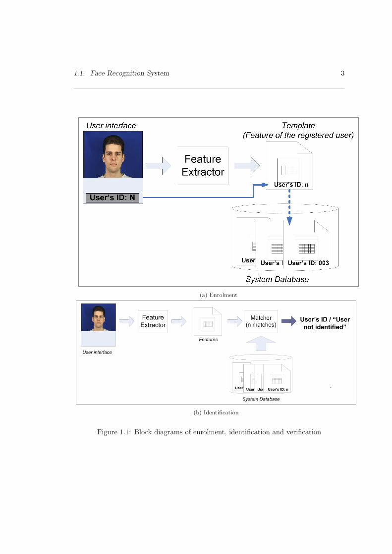
1.1. Face Recognition System 3
(a) Enrolment
(b) Identification
Figure 1.1: Block diagrams of enrolment, identification and verification

4 Chapter 1. Introduction
(c) Verification
Figure 1.1: Block diagrams of enrolment, identification and verification
1.2 Challenges of Face Recognition
Human visual system finds it easy to identify familiar human faces even under severely
degraded viewing conditions, such as viewpoint, illumination, expression, occlusion,
disruption due to accessories and so on. However, automated face recognition is not
yet able to achieve comparable results because measuring the similarity between two
faces is based on the conventional measures of image similarity, such as, Euclidean
metric or Normalised correlation. As Euclidean metric measures the distance between
the images, the smaller the distance the greater the similarity. On the other hand,
Normalised correlation directly measures how similar two images are. It follows that
these two measures are inverse to each other. Figure 1.2 illustrates the inadequacy
of these measures for assessing similarity in face recognition. Image 1 and Image 2
show the same person under even and uneven illumination, while Image 3 shows a
different person. The template is a reference image belonging to the person in Image
1. Table1.1 clearly shows that similarity and distance measures would rate Image 3 to

1.2. Challenges of Face Recognition 5
(a) Template (b) Image1 (c) Image2 (d) Image3
Figure 1.2: Examples of face image
Table 1.1: Conventional similarity measure of those face images in Figure1.2
Image 1 Image 2 Image 3
Normalised Correlation 0.4334 -0.866 -0.2187
Euclidean Distance 4,069 10,033 5424
be more similar to the template than Image 2. This simple test demonstrates that the
similarity measurements fail to generalise in the presence of image degradation.
Zhao et al. [126] and others[31] have discussed extensively the challenges of face recog-
nition which raise issues in mathematics, computing, engineering, psychophysics and
neuroscience. These challenges can be summarised in two points: (1) A large variability
in facial appearance of the same person and (2) High dimensionality of data and small
sample size.
A large variability in facial appearance of the same person is caused by variations of
facial pose, illumination, and facial expression. These variations are further increased
by changes in the camera parameters, such as aperture, exposure time, lens aberrations
and sensor spectral response. As mentioned in [37, 31], the intrapersonal variations
are usually larger than the image variation due to change in the face identity, called
inter-personal. This variability makes it difficult to build a simple model to describe

6 Chapter 1. Introduction
an individual from a small number of sample images or perform linear discriminant
analysis to separate different persons. Mathematically speaking, the face manifold is
highly complicated and non-linear.
High dimensionality and small sample size: In general, the number of samples per
person (typically less than 5) available is much smaller than the dimensionality of the
image space. Therefore, the system cannot build reliable models of each individual
to recognise the face identity from a probe image. This is called the generalisation
problem. In addition, a small sample size may lead to numerical problems in matrix
operations because of the singularity of within class covariance matrices [6]. In gen-
eral, two directions, face image representation and pattern classification based on the
extracted features, must be pursued to deal with these challenges.
1.3 Contributions
The contributions of this thesis to the methodology of face recognition are summarised
as follows:
The thesis presents a Multi-scale local binary pattern histogram (MLBP) for face recog-
nition. The system offers considerable improvement in the recognition performance in
the presence of localisation errors because it benefits from the multiresolution informa-
tion captured by the regional histogram. In the past, the problem associated with a
multiresolution analysis was the high dimensionality of the redundant representation
combined with the small training sample size. These limited the total number of Local
binary pattern (LBP) operators to at most of 3. Our approach, which uses the linear
discriminant analysis (LDA) to reduce the dimensionality and extract the discrimina-
tive information, offers better performance and robustness than the basic local binary
pattern approach for face recognition.
1.3. Contributions 7
The thesis also presents a simple and efficient discriminative descriptor which is de-
rived by a joint color-texture analysis, referred to Multi-spectral local binary pattern
histogram (MSLBP). The descriptor is formed by projecting the local face image ac-
quired by multispectral LBP operators, into LDA space. The overall similarity score
is obtained by fusing the similarity scores of the regional descriptors. This method has
been implemented and compared with other well known benchmarks in the face verifi-
cation. The results on the XM2VTS database clearly show that MSLBPH+LDA+SVM
outperforms other state-of-art contenders.
Illumination is known to be the one of most significant problems in face recognition.
The strategies for tackling this problem can be summarised in two directions. The first
is to convert the face image to a more canonical form in which illumination variations
are suppressed. Other face modalities (such as 3D face shape or near-infrared face im-
ages), photometric normalisation and robust texture descriptor (such as Gabor filters
and LBP) can help for this respect. The second direction is to establish the robust
classifier under illumination variations. In the thesis, the merit of different photomet-
ric normalisation techniques is investigated in the context of LBPH face recognition.
Photometric normalisation is used to reduce the effects of illumination before apply-
ing the LBPH face recognition method. The techniques have been tested on Feret,
XM2VTS darkened and FRGC 2.0 databases. The algorithm that performed well most
consistently is Multi-scale Full Local Binary pattern with LDA in conjunction with
Preprocessing Sequence method [93]. In conclusion, the proposed Multi-scale Local
Binary Pattern histogram system with the Preprocessing Sequence (PS) normalisation
method offers a simple and robust solution to the illumination problem and the pres-
ence of localisation errors for face recognition. Results also show that our proposed
system can achieve comparable performance to the state-of-art systems.

8 Chapter 1. Introduction
1.4 Overview of Thesis
The outline of the thesis is described below.
Overview of Face Recognition: The structure of a generic face recognition is de-
scribed in Chapter 2. Firstly, the existing face recognition systems are categorised
into holistic- and component-based methods. Secondly, the main baseline and
state of art face recognition systems, configured from different processing mod-
ules are summarised. Some of the basic processing stages, including the geometric
and photometric normalisation, the face representation, the feature selection and
extraction, and the classifier are introduced.
Ordinal measures for Face representation: Ordinal contrast encoding for face rep-
resentation has recently become popular because the operation is simple and it
captures the mutual ordinal relationships between neighbours at pixel level or
region level, reflecting the intrinsic nature of the face. In Chapter 3, Ordinal
Contrast Encoding for recognition will first be introduced. Then a structured
local ordinal contrast encoding methods, such as Quadrant Bit Coding, Census
Transform and Local Binary Pattern (LBP), are also described.
Databases: In Chapter 4, three of the well known databases with their common pro-
tocols used in the experiments are first described. Then the measures commonly
used for assessing the performance of face identification and verification systems
are presented.
Advanced Local Binary Pattern Operator: A powerful texture descriptor, called
Local Binary Pattern, and its variants developed for face recognition, have been
introduced. However, these systems, operating in a single scale space, limit the
robustness of the representation to image translation and rotation. Intuitively,

1.4. Overview of Thesis 9
it should be possible to enhance the robustness by extending the representation
method to multiresolution. In Chapter 5, two novel representations, called Multi-
scale LBP (MLBP) and Multispectral LBP (MSLBP), are proposed to extend
the LBP so as to provide a tool for multi-resolution and multispectral analysis of
faces. The resulting LBP methods provide input to LDA and various classifier
fusion methods for face recognition. Experiments are carried out and the results
show that MSLBPH outperforms other state-of-art contenders, while the MLBPH
method is more robust in the presence of localisation errors.
A Comparison of Photometric Normalisation Methods: Illumination is known
to be the one of the most significant problems of face recognition. Photometric
normalisation is important, even if illumination invariant features, such as Gabor
or LBP, are used for face representation as their assumption behind the invariance
property rarely holds. In order to study the merits of photometric normalisation,
five different photometric normalisation methods are implemented. These include
homomorphic filtering, Contrast Limited Adaptive Histogram Equalisation[72],
the Preprocessing Sequence approach[93] and the Retinex approach[23]. These
systems are then tested on the three databases mentioned in Chapter 6. A supe-
rior performance is achieved by MLBPH with the Preprocessing Sequence method
for all the tests. A comparison with the state-of-art systems show that the pro-
posed Multi-scale Local Binary Pattern histogram system with the Preprocessing
Sequence (PS) method can achieve very good performance, while offering a simple
solution which is robust to the localisation errors and illumination changes.
Conclusions and Future Work: The thesis is drawn to conclusion in Chapter 7
where the directions of future work are also suggested.

10 Chapter 1. Introduction
Chapter 2
Overview of Face Recognition
In general, two directions, feature representation and pattern classification based on
the extracted features, must be pursued to deal with the challenges mentioned in Sec-
tion 1.2. The first is concerned with the representation of a face image in a ”good”
feature space where the face manifolds become simpler. Both image normalisation and
face representation can help in this respect. The second direction relates to the design
of a classifier to solve the difficult non-linear classification and regression problems in
the new face space and obtain good generalisation. In other words, the face image is
segmented and then normalised by geometric and photometric normalisations which
eliminate the effect of face rotation in plane, and scaling, and improve the face im-
age quality. Then, a face representation, such as Gabor wavelets which reduce the
non-linear behaviour of face data due to intra-personal variation, is extracted from
the normalised image. Although good normalisation and face representation methods
help in reducing the degree of nonlinearity, commonly the dimensionality of the face
representation is increased. Therefore, an effective dimensionality reduction method
and a classifier are needed to deal with the above problem. The development of a
11

12 Chapter 2. Overview of Face Recognition
successful algorithm requires the exploration of both directions. Many methods of face
recognition pursuing the above directions have recently been proposed. An overview of
all these methods is given in Table 2.1.
Referring to a survey[126], face recognition systems can be grouped in two categories:(1)
structure-based, (2) appearance-based. In structure-based methods[103], a set of geo-
metric face features, such as eyes, nose, mouth corners, is extracted. The position of
the different facial features form a feature vector as the input to a structural classifier to
identify the subject. However, reliable facial feature detection and localisation methods
are essential for this approach to be successful.
Recently, the most systems, as summarised in Table 2.1, use the appearance of face
as the input to decision making and they can be further categorised as holistic and
component based. The holistic appearance methods operate on the global properties
of the face image. In contrast to structural methods, the face representation generally
does not highly rely on accurate detection and localisation of specific facial points, and
therefore these methods are usually more practical and easier to implement. Nowadays,
appearance methods not only operate on the raw image space, but also other spaces,
such as wavelet, local binary pattern and ordinal pattern spaces. One of the reasons
for using alternative face representations is that they simplify the face manifolds. Nev-
ertheless, these kinds of representations exhibit high information redundancy and noise
content, and information compression is needed to reduce the dimensionality of the rep-
resentation to provide a concise and manageable feature space for classification. Several
dimensionality reduction schemes have been developed to discover lower dimensional
representation of human face by relying on statistical regularities. By reducing the
dimensionality, it makes the recognition system also computationally tractable.
In general, good performance of holistic approaches can be achieved with well-illuminated
frontal face images. This is the direct consequence of the majority of algorithms relying
2.1. Generic Face Recognition 13
on fundamentally linear analysis techniques. The performance of holistic approaches
often degrades rapidly with pose changes, uneven illumination, and background clut-
ter. Thus, an alternative to the holistic approach is to base face authentication on
local facial components. The main idea of component-based approach is to increase
the robustness to variations in pose, illumination and to face misalignment by allow-
ing a flexible geometrical relation between the components in the classification stage.
Heisele and his colleagues[25] have evaluated and compared the performance of holistic
and component appearance systems with respect to their sensitivity to pose changes.
Their experiments showed that the component-based system outperforms holistic sys-
tems even though more powerful classifiers are applied in the latter case. On the other
hand, our work[10] and Ahonen et.al[2] also found that component-based approaches
are more robust in the presence of face localisation errors.
In general, there are three traditional schemes to extract facial components. The sim-
plest and most practical schemes[2, 10] divide the whole face image into non-overlapping
or overlapping windows and regard them as the components. Another scheme[63, 25] is
to extract the components centered on the facial features. The last scheme[45] is to ap-
ply the feature selection methods to select the components from a pool of over-complete
local regions obtained by shifting and scaling a window on the face image.
2.1 Generic Face Recognition
Referring to Table 2.1, automated face recognition system is an application of pattern
recognition. A block diagram of a generic face recognition system is presented in Figure
2.1.
Image Sensor: Most current face recognition systems are based on face images cap-
tured in the visible light spectrum. The problem of these images is that the

14 Chapter 2. Overview of Face Recognition
Figure 2.1: Configuration of a generic face recognition
changes in appearance of the same person under different illumination conditions
are larger than the changes due to different identities. This motivated the devel-
opment of various special sensors to obtain different face modalities, such 3D face
shape, near-infrared face images[43, 127], thermal face images, in order to elimi-
nate dependence on illumination conditions. In this work, we focus on 2D image
in the visible light spectrum only because this type of sensor is widely available.
Face Detection: The first step in the face recognition system is face detection. Its
reliability has a major influence on the peformance and usability of a face recog-
nition system. The purpose of this module is to provide the face location data
for the face registration and normalisation module to segment the face region.
Detecting a face in a complicated scene is very difficult because the system needs
a set of reliable features which always appear when a face is present. Over the
years, various methods have been reported. The reader can be referred to [111]
for a comprehensive and critical survey of face detection methods. Up to now,
perfect face localization is very difficult to achieve, and therefore a face recogni-
tion method capable of working well in the presence of localization errors is highly
desired. In our work, the face detection problem is not considered and the face
location data, i.e. eye locations, are assumed. Nevertheless, our systems are also
evaluated in the presence of localisation errors and as we shall see in Chapter 5
our empirical results clearly show that the performance is relatively stable in the
presence of localisation errors.

2.1. Generic Face Recognition 15
Face Normalisation: This module consists of geometric and photometric normalisa-
tion. In general, the photometric normalisation is performed after the geometric
normalisation. The aim of the geometric normalisation is to help the compara-
bility of face images, while the objective of the photometric normalisation is to
eliminate the illumination effects among different images. More comprehensive
description for this module will be presented in Sections 2.1.1 and 2.1.2.
Face representation: As mentioned in Section 1.2, the main disadvantage of using
the intensity image for face representation is its sensitivity to lighting variation,
expression variation and a change of pose. Therefore many researchers have
recently focused on developing more invariant face image representation. The
features in these representations capture the local information that is difficult to
learn using a small set of training data. In Section 2.1.3 and Chapter 3, Gabor
features, ordinal features and Local Binary Patterns will be introduced which do
not depend to the same extent on a large training set being available.
Dimensionality Reduction: The main problem of face recognition methods is the
high-dimensionality of feature space with commonly a small sample size dataset
available for training. A straightforward implementation is computationally ex-
pensive. Therefore, techniques of feature selection or feature extraction are highly
desired. One of the simple feature selection methods is based on the human
perception[103]. In the Elastic Bunch Graph Matching approach, the features
are selected based on specific facial points chosen by a human expert. In Sub-
section 2.1.4, another alternative, Adaboost will be described. Section 2.1.5 will
introduce the techniques of feature extraction.
Classifier: Once the images are projected to a subspace, the similarity of the image
and the template(s) will be measured to determine the person’s identity. Section

16 Chapter 2. Overview of Face Recognition
2.1.6 will discussed this problem in detail.
2.1.1 Geometric Normalisation
Given an image, I, and the eye coordination data, iLeye and iReye, with the predefined
eye coordinates, gLeye and gReye. An affine warp can be applied for geometric normal-
isation. The affine warp equation relating the cropped face image to the image, called
inverse mapping is presented below.
p = Aq + b (2.1)
where p and q are locations of the input image and cropped face image respectively.
A, denoting an affine transform matrix, is obtained below.
A = s×cos(θ) −sin(θ)
sin(θ) cos(θ)
(2.2)
where
θ = ∠(id)− ∠(gd) and s =‖id‖‖gd‖
id = iLeye − iReye and gd = gLeye − gReye
The basis vector, b, presented below is computed based on the midpoints of eye loca-
tions.
b = imid −Agmid (2.3)
where
imid =iLeye + iReye
2and gmid =
gLeye + gReye
2

2.1. Generic Face Recognition 17
Once the parameters of equations, A and b, are calculated, a cropped geometric face
image, G can be obtained by the following equation.
G(q) = I((A−1(p− b)) (2.4)
2.1.2 Photometric Normalisation
The aim of the photometric normalisation is to eliminate the illumination effect among
different images. The techniques can be divided into two groups. The first group uses
training face samples to learn a global model of the possible illumination variations,
for an instance, a linear subspace[6] or an illumination cone[7], which eliminates the
variations seen in the new images. The disadvantage of this group is that it needs many
training samples. The second group is to seek conventional image processing transfor-
mations which remove the influence of illumination variations from face images. The
merit of this group is that they do not require a training stage and training sample.
Contrast Limited Adaptive Histogram Equalisation[128], Histogram Equalisation, Pre-
processing sequence approach[93] and Retinex approach[23], described in Chapter 6,
all belong to this group.
2.1.3 Gabor wavelets
Gabor wavelets were introduced to image analysis because of their similarity to the
receptive field profiles in cortical simple cells. They characterise the image as localised
orientation selective and frequency selective features. Therefore, low level features, such
as peaks, valleys and ridges are enhanced by 2-D Gabor filters. Thus, the eyes, nose
and mouth, with other face details like wrinkles, dimples and scars are enhanced as
key features to represent the face in higher dimensional space. Also, the Gabor wavelet
representation of face image is robust to misalignment to some degree[80] because

18 Chapter 2. Overview of Face Recognition
it captures the local texture characterised by spatial frequency, spatial position and
orientation. The commonly used Gabor filter is defined as follows[103, 81]:
ωu,v(z) =‖ku,v‖2
σ2e−‖ku,v‖2‖~z‖2
2σ2 [eiku,vz − e−σ2
2 ] (2.5)
where u and v define the orientation and scale index of the Gabor kernels, z = [x, y]T ,
‖.‖is the norm operator, and the wave vector ku,v is defined below.
ku,v = kveiφu
where kv = kmaxfv and φu = πu
8 with kmax the maximum frequency, and f being the
spacing factor between kernels in the frequency domain. The term e−σ2
2 is subtracted
to render the filters insensitive to the overall level of illumination. In face recognition,
researchers commonly use 40 Gabor wavelets with five scales v ∈ [0, 5) and eight orien-
tations u ∈ [0, 8) with σ = 2π, f =√
2 for half octave spacing, kmax = π2 for 128× 128
images size[103, 116] and kmax = π for 64× 64 images size.
Gabor image, Gu,v(z) ∈ C, is generated by taking the convolution of face image, I(z),
and Gabor wavelet, ωu,v(z). The convolution process can be taken in the Fourier
domain for fast computation. In the face recognition community, many researchers[85,
103, 116, 52, 50, 39, 89, 81, 90, 3] have widely used the magnitude of Gabor filters for face
representation. Most recently, Shan et.al.[116, 73] have proposed Gabor phase patterns
histogram by encoding the Gabor phase information for face representation. On the
other hand, Jones et.al [33] have extended the Gabor function to the hypercomplex
domain for color face recognition.
2.1.4 Feature Selection
Recently, boosting algorithms have been widely accepted by the face research commu-
nity. One of the reasons is that a boosting algorithm is a majority voting classifier.
2.1. Generic Face Recognition 19
Face recognition is a multi-class problem, but binary Adaboost can only solve the two
class problem. To avoid the need for a complex training process, the training samples
can be remapped to intra-personal and inter-personal differential populations. An ideal
intra-personal difference is an image with all pixel values set to zero, while an inter-
personal difference should have much larger pixel values. Several ways of implementing
this mapping have been suggested in the literature[101, 59]. In the Gabor feature
space[121], the positive examples are derived from the pair of intrapersonal differences
on the magnitude images and phase images in their corresponding scale and orientation
space, whereas the negative samples are from the pair of interpersonal differences.
In the LBP histogram[46], an image pair is first split into sub-regions. The similarity
score of each local LBP histogram pair is measured using the similarity function which
will be discussed in Section 5.3. The similarity scores are then concatenated to form
an input feature vector for feature selection process. Over-complete features[120] can
be provided by shifting and scaling the local regions. In general, the total sample size
of inter-person pairs is larger than that of intra-person pairs. This will give rise to a
bias for feature selection. There are two approaches to solve this problem. One is to
employ multiple feature selectors, each of them using the whole set of intra-person sam-
ples with a portion[14] of the inter-person samples determined by randomly sampling.
Another[112, 4, 81, 99] is to devise a cascaded Adaboost system with predefined false
positive rate and detection rate (or called recognition rate) in each stage, and a prede-
fined final false positive rate. The sample size ratio of intra-person pairs to inter-person
pairs is fixed in each stage, and therefore inter-person samples are randomly sampled
in the pool. In each stage after the training phase, evaluation samples are involved
to measure the false positive rate of the strong classifier so as to fulfil the predefined
detection rate in decreasing the threshold in the last stage of the strong classifier. If
the false positive rate does not meet the predefined rate, the Adaboost feature selec-

20 Chapter 2. Overview of Face Recognition
tion process will be iterated. Otherwise, the misclassified inter-person samples in the
current stage, the full set of intra-person sample will be used to design the next stage of
the cascaded classification process. If the inter-person samples do not meet the sample
size ratio, the remain will be added by randomly sampling in the pool. The process
is iterated until the false positive rate meets the predefined final false positive rate.
After that, the selected features will be stored. A final strong classifier is formed by
combining a number of weak classifiers. For the detail of the AdaBoost based feature
selection process or classifier, please refer to [78]. A summary of the AdaBoost process
is shown below.
- Given a training set with m samples: (x1, y1), . . . (xm, ym) where xi ∈ Rn =
[x1 . . . xn]t, yi ∈ Y = {−1, 1}.
- Initialise weights: w1(i) = 1m , i ∈ [1,m]
- For t = 1, . . . , T
1. Find and store the classifier ht : Rn −→ {−1, 1}, which minimises the error
εj |j ∈ [1, n] with respect to the weight distribution wt:
ht = arg minhj∈H
εj , where εj =m∑
i=1
wt(i)[hj(xi) 6= yi]
2. Prerequisite: εt < 0.5, otherwise stop.
3. Choose and store αt = 0.5 ln(
1−εtεt
), where εt is the weighted error rate of
classifier ht.
4. Update the weight distribution:
wt+1(i) =wt(i)Zt
×
e−αt if ht(xi) = yi
e+αt if ht(xi) 6= yi
where Zt is a normalisation factor, such that∑m
i=1 wt+1(i) = 1.

2.1. Generic Face Recognition 21
• Define the final strong classifier as:
H(x) = sign
(T∑
t=1
αtht(x)
).
2.1.5 Feature Extraction
Classification methods operating in the image-space or feature-space representation
suffer from a number of potential disadvantages, most of which root in the curse of
dimensionality. However, most of the face surface is smooth and has regular texture.
A pixel value is typically highly correlated with the values of the surrounding pixels.
Moreover, the face appearance is highly constrained; for example, the frontal view of a
face is roughly symmetrical. Thus the natural constraints dictate that the face images
are confined to a subspace. To solve the curse of dimensionality problem, the feature
selection, mentioned in Section 2.1.4, and the feature extraction in the current section
can assist to reduce the dimensionality. The feature extraction methods can be linear or
nonlinear. They project the high-dimensional raw vector, x ∈ Rn such as concatenated
pixels in the image space, feature space or selected feature space, into a low dimensional
space in which a new feature vector, y ∈ Rv is given as.
y = WTx
where W ∈ Rn×v is a transformation matrix. In this section, linear combination
methods such as the well known Principle Component Analysis (PCA) and Linear
Discriminant Analysis (LDA) will be described.
PCA
PCA is a standard decorrelation technique which projects the input signal into a space
where features have no correlation with each other. It is a common technique for signal
22 Chapter 2. Overview of Face Recognition
representation or signal compression because PCA can reduce the dimensionality by
keeping the space which encapsulates the maximum amount of signal variation and
throwing out dimensions with small variation which are regarded as noise. Pentland
et al. [36] applied PCA to face recognition and called the face subspace as Eigenfaces.
In PCA-based training algorithm, the input is a training set, X = [x1, . . . ,xm] of m
facial images such that the mean of the training set is zero. The dimension of x is the
total number of features used for describing the face. The PCA axes are found by the
eigen-analysis of the training set covariance matrix, i.e.
ΣxΨ = ΨΛ (2.6)
where Σx ∈ Rn×n = 1m
∑mi=1 (xixi
T ) = 1mXXT , Ψ = [ψ1, . . . , ψn]T is the matrix of
eigenvectors of the train set covariance matrix, Σx, and Λ is the diagonal matrix with
eigenvalues λ1 ≥ . . . λn on its main diagonal, so ψj is the eigenvector corresponding to
the jth largest eigenvalue. Then it can be shown that the eigenvalue λi is the variance of
the data projected on ψi. Thus, the lower order eigenvectors encode to larger variations
of the training set, while the higher order eigenvectors encode smaller variations of the
training set. As reported by Zheng[102], ordering eigenvectors based on the descending
order of eigenvalues is good to represent or compress the information, but it may not
be good for signal classification. Thus, the eigenvectors can be reordered based on the
distance between image pairs of the same persons projected into Eigenspace, so-called
Like-image different ordering[109].
In general, some portion of the higher-order eigenvectors is removed because it does
not contribute to face recognition and the computation time can also be saved. There
are six variants of eigenvector selection as shown below.
Standard eigenspace projection[109]: All eigenvectors corresponding to non-zero
eigenvalues are kept to establish the subspace.

2.1. Generic Face Recognition 23
Remove the last 40% of the eigenvectors[29]: The eigenvectors are sorted by the
corresponding descending non-zero eigenvalues and this method only keeps 60%
of the lower-order eigenvectors.
Energy dimension[109]: This method uses the minimum number of eigenvectors to
guarantee that the retained energy is greater than a threshold. A typical threshold
is 0.9. The PCA and LDA functions in our RAVL library adopt this method to
choose the eigenvectors. The energy, ei, of the ith eigenvector is the ratio of the
sum of the first i eigenvalues over the sum of all the eigenvalues.
ei =
∑ij=1 λj∑nj=1 λj
(2.7)
Stretching dimension[109]: The stretch of eigenvector is another method to select
the eigenvector. The stretch, Si, of the ith eigenvector is the ratio of the ith
eigenvalue, λi, over the maximum eigenvalue , λmax. A common threshold for the
stretching dimension is 0.01.
Si = λi/λmax (2.8)
Removing the first three lower-order eigenvectors[109]: The previous methods
assume that the recognition is affected by the information in the higher order
eigenvectors. However, Moon. et al. [29] stated that the lighting effects can be
eliminated by removing the lower-order eigenvectors.
Genetic Algorithm[102]: Zheng et al. stated that some higher-order eigenvectors
should also be used as a part of the basis for dimension reduction for improving
the recognition performance. Therefore a Genetic Algorithm is applied to solve
the problem of eigenvector selection.
On the other hand, if the sample size is much smaller than the dimensionality, m << n,
which means that the number of non-zero eigenvalues is less or equal to sample size
24 Chapter 2. Overview of Face Recognition
(m) , then the following method can reduce the computation from O(n) to O(m)
(XTX)Φ = ΦΛ1
Ψ = XΦ(2.9)
where Λ1 ∈ Rm×m is a diagonal matrix with eigenvalues, λ1 ≥ . . . λm on the diagonal,
and Ψ ∈ Rn×m = [ψ1, . . . , ψm]T .
After the eigenvector selection, the new transformation matrix is defined as Wpca =
[ψ1, . . . , ψv], and the new feature vector y with lower dimensionality v is computed as
y = WpcaTx (2.10)
LDA
Although the eigenface method is useful to represent the face image, there is no reason to
assume that this method enhances face recognition and the majority of face recognition
papers have already argued this point. Motivated by this observation Belhumeur et
al. [6] proposed the class specific linear method, called Fisher’s Linear Discriminant
analysis, FLD, to achieve better face recognition. The theoretical framework for the
FLD is to maximise the ratio of between-class scatter to that of within-class scatter.
Let the between-class scatter matrix be defined as
Sb =C∑
i=1
ni(ui − u)(ui − u)T (2.11)
And the within-class scatter matrix be defined as
Sw =C∑
i=1
∑
x∈Ai
(x− ui)(x− ui)T (2.12)
where ui is the mean of face images from class Ai, C is the total number of classes and
ni is the number of samples in class Ai. If Sw is non-singular, the optimal projection,
2.1. Generic Face Recognition 25
WLDA, is chosen as the matrix which maximises the equation below.
WLDA = arg maxW
|WSbWT ||WSwWT | (2.13)
In the case of face recognition, the number of images in the training set m is much
smaller than the number of pixels in the image, n, making the within-class scatter
matrix singular. This means that it is possible to choose matrix W such that the
within-class scatter of the projected samples is zeros. In recent years, many solutions
have been proposed to tackle this problem. Belhumeur et al. have proposed the method
called Fisherface, which avoids the problem by projecting the image set to a lower di-
mensional space so that the resulting within-class scatter matrix is non-singular. This
process is done by using PCA to reduce the dimension of the feature space so that the
within-class scatter in the PCA space is non-zero, and then using the standard FLD to
reduce the dimension to C-1. In order to improve the generalisation capability of FLD,
other researchers[47, 15, 119] have suggested the Enhanced Fisher Linear Discriminant
Model (EFLDM). This method decomposes the FLD procedure into a simultaneous
diagonalisation[20] of the two within- and between-class scatter matrices. It first di-
agonalises the within-class scatter matrix and then the between-class scatter matrix.
With this approach, more discriminating features in the PCA space can be kept for
EFLDM.
Chen et al. [13] have developed a new LDA-based face recognition, called Null Space
LDA (N-LDA), which can solve the small size problem. It chooses the projection
vectors (transformation matrix) maximising between-class scatter with the constraint
that the within-class scatter is zero, as the null space of a within-class scatter matrix has
been shown containing discriminative information. In a similar vein, Yu and Yang[114]
proposed the so called Direct LDA (D-LDA). The key idea is to discard the null space of
between-class scatter which contains no useful first order information. This process can
be achieved by diagonalising the between-class scatter matrix and then diagonalising
26 Chapter 2. Overview of Face Recognition
the within-class scatter matrix. Recently, Ye and Li[113] have suggested a two-stage
FDA via the QR-decomposition. The first stage of the QR decomposition method, as
a dimension reduction, maximises the separation between different classes. The second
stage of QR is to perform FDA.
Other Subspace methods
Other subspace methods, such as Independent Component Analysis (ICA), Kernel
PCA(KPCA), Kernel LDA (KDA), Discriminant Common Vector Approach (DCV)
and Discrete Cosine transform (DCT) have been proposed. KPCA and KLDA are the
kernel versions of PCA and LDA where a nonlinear mapping is applied to the original
space before a PCA or LDA projection. In ICA, a non-orthogonal transformation is
selected such that the variables in the feature space are statistically independent.
2.1.6 Classifier
The goal of a classifier is to compare the features of a face probe image with those
of the template and report the degree of match in terms of some match or similarity
measure. Since face recognition is a multiclass problem often involving a small sample
size, most systems apply a Nearest Neighbor(NN) classifier to make the decision. An
important issue of the NN classifier design is how to measure similarity. In general,
there are two ways to measure similarity. One is to measure the distance between the
image features. The second possibility is to measure how similar they are. These two
measures are the inverse of each other. There are many possible similarity and distance
measures and some of them are presented below.
L1 norm:
d =n∑
i=1
|xi1 − xi
2| (2.14)

2.1. Generic Face Recognition 27
where xi1 and xi
2 are an i-th element of vectors x1 and x2 respectively.
L2 norm:
d = ‖x1 − x2‖ =√
(x1 − x2)T (x1 − x2) (2.15)
Mahalanobis distance:
d =√
(x1 − x2)TA−1(x1 − x2) (2.16)
Normalised Correlation:
d =xT
1 x2
‖x1‖‖x2‖ (2.17)
Mabalanobis Angle:
d =xT
1 A−1x2√xT
1 A−1x1
√xT
2 A−1x2
(2.18)
where A is the covariance matrix. After PCA, A is a diagonal matrix defined by the
eigenvalues of the original covariance matrix.
Some researchers have applied other classifiers, such as SVM, or boosting classifier, for
recognition. These are naturally defined as two-class discriminant classifiers. There
are two approaches to convert the multiclass problem into a binary problem. The first
approach, called intra-interpersonal difference method, is to evaluate the difference
between two images as a basis for determining whether the images are of the same
person. The second approach, called client-specific method or one-vs-all method, is to
establish classifiers each of which separates a single class from all remaining classes.
In the component-based approach, there are two ways to perform the classification.
The simplest and the most practical one, called score-based classifier, is to build a
classifier for each component and then combine the output scores by applying fusion
techniques. The second method, called feature-based classifier, is to apply a single
classifier on the component features. Researchers[26, 75, 60] applied a Hidden Markov
Model(HMM) classifier or Gaussian mixture models(GMM) classifier in which the fea-
tures of components, such as features located on the eyes, chin and mouth regions,
28 Chapter 2. Overview of Face Recognition
are represented by a multivariate probability distributions. Tan and his colleagues[94]
concatenate the features of individual components into a single feature vector, and then
apply the technique of dimensionality reduction to determine the final discriminative
feature vector.
2.2 Summary
Generic face recognition systems can be classified as structure-based or appearance-
based. Recently, the appearance-based approach has been used in most of the face
recognition systems. In this chapter, the appearance-base methods have further been
categorised into holistic- and component-based methods. The main baseline and state
of art face recognition systems, configured from different processing modules are sum-
marised in Table 2.1. Face recognition is a multiclass problem and potentially re-
quires a vast quantity of training data to design. This problem is mitigated by the
intra-interperson difference approach and the client-specific approach, described in this
chapter, which transforms the multiclass problem to a more manageable binary prob-
lem. In order to improve the performance of automatic face recognition, the techniques
of face representation and pattern classification have been introduced to simplify the
human face manifold. Lately, researchers have focused on developing a face represen-
tation capturing the local information which achieves invariance to facial expression
and illumination. Motivated by a simple but powerful texture descriptor, called Local
Binary Pattern, our proposed system extends this descriptor to multiresolution and
multispectral analysis for face recognition. The results presented in Chapthers 5 and 6
clearly indicate that our proposed systems can achieve comparable performance to the
best of state-of-art systems.

2.2. Summary 29
Table 2.1: Survey of face recognition methods
Ref. Face RepresentationDimensionality Reduction
ClassifierFeature Selection Feature Combina-
tion
Holistic-
Appearance
based
Approaches
[6, 30, 64,
98]
Image Space
PCA
Nearest
Neighbour[6, 13, 35,
110, 104,
114, 37,
113]
LDA
[5] ICA
[106] LPP
[34, 25] PCA, LDA CS-SVMs
[12] Random Subspace PCA, LDA Multiple Classi-
fiers
[59, 95] Intra/Inter diff.
sets in image space
PCA Bayesian Classi-
fier
[108] MRC-AdaBoost
[66] Intre and Inter. difference sets in PCA space SVM
[103]
Gabor Mag. Space
Automated facial
point detection and
localisation
Nearest
Neighbour
[22] Shape context
[50, 83,
117, 51]
LDA, KFA, GDA,
KDA, PCA
[118] LDA CS-SVMs
[105, 4] AdaBoost, Multi-
boost
GDA, DS-LDA Nearest Neigh-
bour
[112, 81,
84]
Intra/Inter diff.
sets in Gabor Mag.
space
boosting classifier
[121, 73] Intra/Inter diff. sets
in Gabor Phase
space
boosting classifier, Bayesian Classifier
Local-
Appearance
based
Approaches
[17]
Image Space
DCT
Score Classifier[36] LDA
[63, 41] PCA
[86] CS-LDA
[60] DCT HMM
[25] CS-SVMs
[90, 88]Gabor Mag. Space
Adaboost
LDAScore Classifier
[89]
[116] Gabor Phase Pat-
tern Histogram
space
[26] LBP space DCT HMM
[2, 124, 40]
LBP Histogram
space
Score Classifier[24] Adaboost
[10, 11,
125, 44]
KDA, LDA
[75] GMM
[27, 45, 44] Boosting methods

30 Chapter 2. Overview of Face Recognition
Chapter 3
Ordinal measures for Face
representation
In face detection and recognition methods, employing features that mimic the model of
primary visual cortex has been found to be useful. The receptive fields of cells in the
primary visual cortex can be well modelled by Gabor wavelets. Given these wavelets,
there are various ways they can be used to extract measurements from an image to
perform recognition. In face recognition, researchers commonly use 40 Gabor wavelets
with five scales and eight orientations. Each wavelet has a unique orientation, frequency
tuning and scale. The set of wavelets is meant to simulate the multi-scale nature of
the receptive field. From recognition point of view, a bank of Gabor wavelet filters also
provides a wealth of information about each pixel, rather than just scalar response.
However, one of the disadvantages of such multiple wavelet representation is that the
computation cost is high. Therefore, simple local features, derived using Boxlets or
haar-based wavelets, have been proposed for detection and recognition as an alternative.
The mother wavelet is formed by the difference between the sums of the image intensity
31

32 Chapter 3. Ordinal measures for Face representation
values in adjacent rectangular windows. By scaling and shifting the wavelet over the
face image, an overcomplete set of features can be extracted. This overcomplete feature
set helps to capture as much ad-hoc information and knowledge about the domain as
possible, as it would be difficult to learn optimal representation using training data of
finite size. The success of these representations emanates from the use of contrast energy
and multi-scale information captured by these filters. Nevertheless, an alternative novel
method namely ordinal contrast encoding has recently become popular as it not only
gives better face representation than the boxlets, but also the computational cost is
lower than that of the Gabor wavelets. In this chapter, Ordinal Contrast Encoding for
recognition will first be introduced. Then a structured local ordinal contrast encoding,
also known as Local Binary Pattern (LBP) will be described. Techniques of encoding
the patterns such that the representation becomes robust to face misalignment will be
mentioned in Section 3.3. Lastly, the summary of this chapter will be presented.
3.1 Ordinal Contrast Encoding
Ordinal contrast measure comes from a simple concept we always use in our daily life.
For example, we always choose water to drink from a cup by feeling the tempera-
ture rather than measuring its precise temperature. In most cases, however, we are
only interested in a relative difference rather than the precise value. The same thing
also applies to biological and artificial recognition systems. In the visual domain [77],
many striated cortical cells have rapidly saturating contrast response functions. Their
tendency to reach the maximal response at low contrast values implies the cells are
sensitive to local ordinal rather than metric relations. In computer vision, the absolute
information, including intensity, colour and texture, associated with a face can vary
dramatically under various illumination conditions, but the mutual ordinal relation-

3.1. Ordinal Contrast Encoding 33
ships between neighbours at pixel level or region level reflect the intrinsic nature of the
face, and thus provide a degree of response stability in the presence of such changes.
An ordinal contrast encoding is used to encode the contrast polarity of values between
a pixel pair (or average intensities between a region pair) as either brighter than (1) or
darker than (0) some reference. Similarly, it can also be used to encode the contrast
magnitude as either above threshold for 1 or below for 0. The code is efficient to
compute and the information entropy of the measure is maximised because the code
has nearly equal probability of being 1 or 0 for arbitrary patterns. To illustrate the
manner in which ordinal contrast measure tolerates various illumination conditions,
such as image gain, bias or gamma correction, consider a three by three region, S of an
image whose intensities are
128 8 210
10 113 60
7 20 A
where A is the pixel value whose range is between 0 and 255. Consider the effect of
this pixel on various parametric or non-parametric measures, computed at the centre of
this region as A varies over its 256 possible values. The mean of this region varies from
61.78 to 90.1, and the variance ranges from 4853 to 8676.4. The mean and vaiance
exhibit contiuous variation over a substantial range as A varys. For the purpose of
encoding the image region S into a binary format, all neighbours in S are compared
with the centre value, 113. If the value in S is greater than the threshold, the code will
be assigned value 1, otherwise it is 0. Then the result, R will be
1 0 1
0 0 0
0 0 a
The rank of R will be 2 no matter A is larger or smaller than 113. This comparion
34 Chapter 3. Ordinal measures for Face representation
clearly shows that the ordinal contrast encoding is more stable. The minority of pixels
in the image, S, can have a very different value, but the effect on the ordinal contrast
relationship is limited by the size of minority. Moreover, R presented above will not
change, even if S is biased, scaled or after gamma correction. In other words, an ordinal
contrast measure applied to S will be invariant to any monotonic transformation of the
gray scale.
R ≡ T (S) ≡ T (S + a) ≡ T (S× a) ≡ T (Sa) | T (:) is ordinal contrast encoding.
(3.1)
Sinha[87] was the first to mention ordinal contrast encoding for face detection. This
method is based on the fact that a set of ordinal contrast measures on face images,
such as eye-forehead region pair, eye-nose region pair and mouth-chin region pair, are
invariant to different persons and illumination conditions. His face detector achieved
a higher detection rate with lower false acceptance rate, which means that ordinal
contrast features have excellent separability between the face and non-face classes.
In order to extract the ordinal contrast information conveyed by a region pair, the
use of a differential operator, namely dissociated dipole filter has been proposed. A
dissociated dipole filter has an excitatory and inhibitory lobes, but the limitation on
the relative position of the two lobes is removed. Thus, it is able to capture non-
local information, such as the information between eye and mouth. There are three
parameters for this filter, and they are the width of the lobes, distance between the
lobes and the orientation angle between the lobes. By tuning these three parameters,
an overcomplete filter set can be obtained. The ordinal contrast feature is encoded by
measuring the polarity of the filter output. By applying feature selection algorithms, a
set of discriminative ordinal contrast features that are tolerant to noise and changes in
illumination conditions can be selected. Nevertheless, Thoresz[96] wondered whether
this kind of feature will be good enough for the recognition.
3.2. Structured Ordinal Contrast Encoding 35
Liao et al. [48] have proposed the use of ordinal measure on the output of complex
differential operator, namely multi-pole filter, for face recognition. In contrast to the
dissociated dipole filter, the multi-pole filter can capture more complex image micro-
structures. A multi-pole filter is designed for a specific macro-structure by using appro-
priate lobe shape configuration. The algorithm is similar to the Shinha method which
applies a boosting algorithm to select a discriminative set of ordinal contrast features
and uses the Hamming distance to measure similarity for face recognition. This system
clearly shows that utilising a set of complex differential operators with ordinal encoding
can provide a powerful discriminative feature for the recognition[92, 48].
3.2 Structured Ordinal Contrast Encoding
Notwithstanding the above methods, there are alternative solutions to obtain a feature
that captures complex information. These methods convert a set of simpler differential
filter outputs to a binary pattern to represent a complex image micro-structure.
3.2.1 Quadrant Bit Coding
Daugman[16] implemented this particular approach for iris recognition. The ordinal
encoding method is applied to the demodulated phase information adapted as an iris
feature. The score of similarity between the input iris image and the registered template
is expressed in terms of the Hamming distance between their iris features. In his
approach, the even and odd Gabor functions are the differential operators used for
detecting blob and edge information. The convolution of an iris image with Gabor
function is equivalent to comparing the intensities of the image regions covered the
excitatory lobes of the Gabor function and the adjacent regions covered by inhibitory
lobes. The output result is further encoded into 1 or 0 depending on its polarity. Thus,
36 Chapter 3. Ordinal measures for Face representation
each pixel in the iris image is encoded into a two bits [BReu,v(z),B
Imu,v(z)] string, shown in
Equ(3.2) and (3.3), which is based on concatenating the ordinal measures devised from
even and odd Gabor outputs,[GReu,v(z),G
Imu,v(z)]. For the details of Gabor wavelets, the
reader is referred to Section 2.1.3.
BReu,v(z) =
0 if GReu,v(z) > 0
1 if GReu,v(z) ≤ 0
(3.2)
BImu,v(z) =
0 if GImu,v(z) > 0
1 if GImu,v(z) ≤ 0
(3.3)
and it can be reformulated as follows:
BReu,v(z) =
0 if φu,v(z) ∈ {I, IV }
1 if φu,v(z) ∈ {II, III}(3.4)
BImu,v(z) =
0 if φu,v(z) ∈ {I, II}
1 if φu,v(z) ∈ {III, IV }(3.5)
This two bits string defined in Equ(3.2) and (3.3) is also called quadrant bit coding
because it indicates the quadrant in which the Gabor phase angle lies. Figure 3.1,
Equ(3.4) and (3.5) clearly show the meaning of the encoding. The quadrant bit coding
is relatively stable and therefore it is one of the reasons behind its successful application
to iris recognition[16] and face recognition[116].
3.2.2 Census Transform
The computation cost of complex differential operators, such as Gabor wavelet and
multi-pole filter, is high, and thus using simpler and more efficient differential oper-
ator is highly desirable. The simplest and surprisedly efficient method is to measure

3.2. Structured Ordinal Contrast Encoding 37
Figure 3.1: Quadrant bit coding of Gabor phase
the difference between two pixels. For this purpose, Zabih et.al[115] have proposed
the Census transform to map the local neighbourhood surrounding a pixel to a bit
string, for computing the visual correspondence. The Census transform presented in
Equ(3.6) is a non-parametric transform which maps the ordinal contrast measures be-
tween neighbours, gp|p ∈ [0, P ) and the centre pixel, gc, to a P-bit string.
C(x, y) = ⊗P−1p=0 s(gp − gc) (3.6)
where P is the total number of pixels in the local neighbourhood, ⊗ is a concatenate
function to join a binary bit to a string, and,
s(x) =
1 if x ≥ 0
0 if x < 0
Each pixel in the Census transformed image is a P-binary string, which captures the
image micro-structure and achieves invariance to any monotonic transformation of the
gray scale. The correspondence between two images is measured by finding the min-
imal Hamming distance between two transformed pixels. This method is particularly
suitable to the application of localising an object because the distance will be zero if
38 Chapter 3. Ordinal measures for Face representation
two Census transformed images share the same binary pattern. However, it is not good
for face recognition or texture recognition because the binary pattern is generated at
the pixel level where the similarity measure will be degraded when one of the images
during comparison is rotated or translated. To compensate for this problem, one of
the solutions mentioned in Section 3.1 and 3.2.1 is to compute the ordinal contrast
measure at a region level, for example, using a regional differential operator, such as
multi-pole filters, Gabor wavelets or edge operators. An alternative solution is based
on measuring the similarity between the histograms of the Census transformed images.
The advantage of applying histogram is that it is invariant to translation.
3.2.3 Local Binary Pattern
Approximately at the same time, the local binary pattern (LBP), the generalised ver-
sion of Census transform, introduced by Pietikainen et al. [70], offers a powerful and
attractive texture descriptor showing excellent results in terms of accuracy and com-
putation complexity in many empirical studies. The most prominent limitation of the
Census transform operator is its small spatial support area. A feature computed using
a 3× 3 operator, only relating to a small image structure, that may not necessarily be
adept to capturing the key texture characteristic. However, LBP using circular neigh-
bourhoods and linearly interpolating the pixel values allows the choice of any radius,
R, and number of pixel in the neighbourhood, P , to form an operator, which can model
large scale structure. An illustration of the basic LBP operator is shown in Figure 3.2
and the corresponding equation is shown below.
LBPP,R(x, y) =P−1∑
p=0
s(gp − gc)2P (3.7)
The LBP has been extended to multiresolution analysis [54], colour texture analysis

3.2. Structured Ordinal Contrast Encoding 39
Figure 3.2: The basic of LBP Operator
[55] and spatio-temporal texture analysis [124]. The LBP and its extensions has already
been applied for instance to visual analysis, image retrieval, motion detection, remote
sensing, biomedical image analysis, and outdoor scene analysis. A descriptor for texture
analysis is a histogram, h(i), of the local binary pattern shown in Equ(3.8) and its
advantage is that it is invariant to image translation.
h(i) =∑x,y
B(LBPP,R(x, y) = i) | i ∈ [0, 2P − 1], B(v)
1 when v is true
0 otherwise(3.8)
Moreover, grouping the patterns based on different criteria, such as Rotation Invariant
LBP, Uniform LBP and Statistically effective LBP, to form a histogram may provide
better discrimination in comparison to the histogram of all individual patterns. The
reason is that the occurrence of some patterns in LBPH is so infrequent that the
probabilities cannot be reliably estimated.
Rotation Invariant Local Binary Pattern
When an image is rotated in plane, the neighbourhoods, gp around the centre pixel,
gc, will be rotated in the same direction. This rotation effect will result in different

40 Chapter 3. Ordinal measures for Face representation
LBPP,R value. To remove a rotation effect, a circular bit-wise right shift operator,
ROR(:), is applied to iterate P times in order to find the minimal decimal value of the
binary pattern. The rotation invariant LBP operator, LBP riP,R, mentioned in [71] is
defined as.
LBP riP,R(x, y) = min {ROR(LBPP,R(x, y), i) | i ∈ [0, P − 1]} (3.9)
Uniform Local Binary Pattern
A subset of these 2P binary patterns, called uniform patterns defined in [53], can be
used to represent spot, flat area, edge and corner. The uniformity measure, U(x),
presented in Equ(3.10) records the number of spatial transitions in the binary pattern,
and the uniform pattern which contains at most two bitwise transitions, i.e., U(x) ≤ 2.
The uniform pattern contains in total (P − 1)P + 2 binary patterns. It consists of
two types of patterns, namely (P − 1)P rotational patterns, such as edges and two
non-rotational patterns, such as a bright spot or a flat area. Other patterns, where
U(x) > 2, are regarded as non-uniform patterns. The uniform LBP operator, LBP u2P,R,
is defined as.
LBP u2P,R(x, y) =
I(LBPP,R(x, y)) if U(LBPP,R) ≤ 2, I(z) ∈ [0, (P − 1)P + 2)
(P − 1)P + 2 otherwise(3.10)
where
U(LBPP,R) = |s(gP−1 − gc)− s(g0 − gc)|+P∑
p=1
|s(gp − gc)− s(gP−1 − gc)|
Superscript u2 shown in Equ(3.10) indicates that the definition relates to uniform
patterns with a U value of at most 2. If U(x) is smaller than 2, the current pixel will
be labelled by an index function, I(z). Otherwise, it will assigned value (P − 1)P + 2.
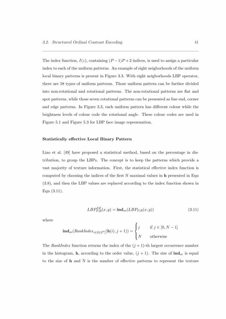
3.2. Structured Ordinal Contrast Encoding 41
The index function, I(z), containing (P −1)P +2 indices, is used to assign a particular
index to each of the uniform patterns. An example of eight neigborhoods of the uniform
local binary patterns is present in Figure 3.3. With eight neigborhoods LBP operator,
there are 58 types of uniform patterns. Those uniform pattern can be further divided
into non-rotational and rotational patterns. The non-rotational patterns are flat and
spot patterns, while those seven rotational patterns can be presented as line end, corner
and edge patterns. In Figure 3.3, each uniform pattern has different colour while the
brightness levels of colour code the rotational angle. These colour codes are used in
Figure 5.1 and Figure 5.3 for LBP face image represenation.
Statistically effective Local Binary Pattern
Liao et al. [49] have proposed a statistical method, based on the percentage in dis-
tribution, to group the LBPs. The concept is to keep the patterns which provide a
vast majority of texture information. First, the statistical effective index function is
computed by choosing the indices of the first N maximal values in h presented in Equ
(3.8), and then the LBP values are replaced according to the index function shown in
Equ (3.11).
LBPSEP,R(x, y) = indse(LBPP,R(x, y)) (3.11)
where
indse(RankIndex i∈(0,2P ](h(i), j + 1)) =
j if j ∈ [0, N − 1]
N otherwise
The RankIndex function returns the index of the (j + 1)-th largest occurrence number
in the histogram, h, according to the order value, (j + 1). The size of indse is equal
to the size of h and N is the number of effective patterns to represent the texture
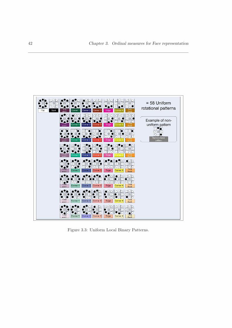
42 Chapter 3. Ordinal measures for Face representation
Figure 3.3: Uniform Local Binary Patterns.
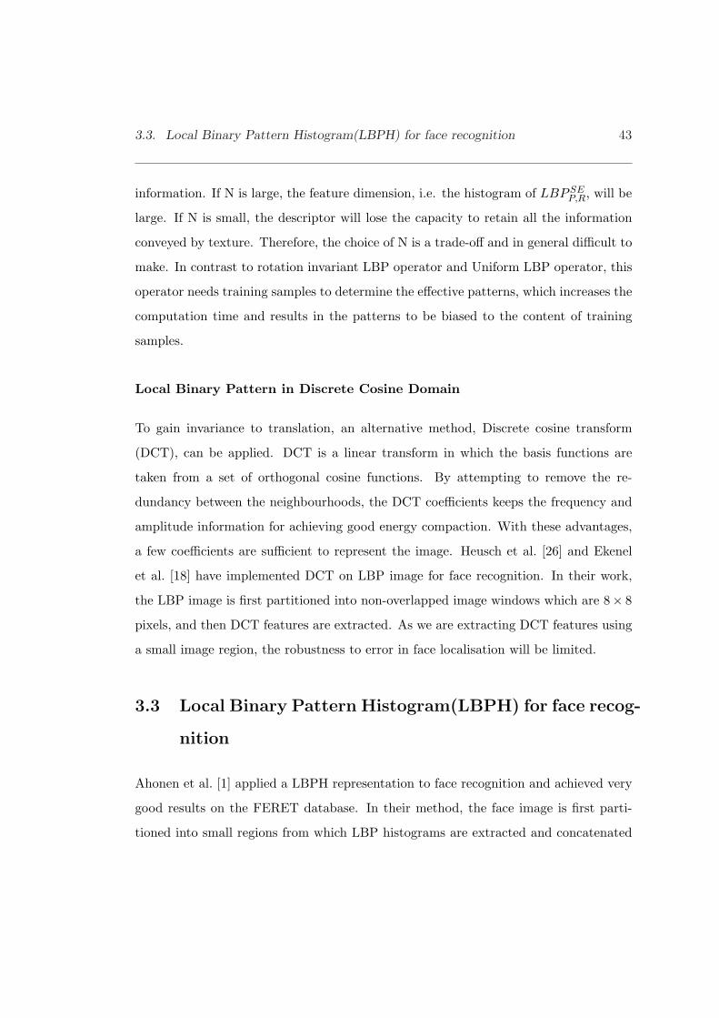
3.3. Local Binary Pattern Histogram(LBPH) for face recognition 43
information. If N is large, the feature dimension, i.e. the histogram of LBPSEP,R, will be
large. If N is small, the descriptor will lose the capacity to retain all the information
conveyed by texture. Therefore, the choice of N is a trade-off and in general difficult to
make. In contrast to rotation invariant LBP operator and Uniform LBP operator, this
operator needs training samples to determine the effective patterns, which increases the
computation time and results in the patterns to be biased to the content of training
samples.
Local Binary Pattern in Discrete Cosine Domain
To gain invariance to translation, an alternative method, Discrete cosine transform
(DCT), can be applied. DCT is a linear transform in which the basis functions are
taken from a set of orthogonal cosine functions. By attempting to remove the re-
dundancy between the neighbourhoods, the DCT coefficients keeps the frequency and
amplitude information for achieving good energy compaction. With these advantages,
a few coefficients are sufficient to represent the image. Heusch et al. [26] and Ekenel
et al. [18] have implemented DCT on LBP image for face recognition. In their work,
the LBP image is first partitioned into non-overlapped image windows which are 8× 8
pixels, and then DCT features are extracted. As we are extracting DCT features using
a small image region, the robustness to error in face localisation will be limited.
3.3 Local Binary Pattern Histogram(LBPH) for face recog-
nition
Ahonen et al. [1] applied a LBPH representation to face recognition and achieved very
good results on the FERET database. In their method, the face image is first parti-
tioned into small regions from which LBP histograms are extracted and concatenated

44 Chapter 3. Ordinal measures for Face representation
into a single, spatially enhanced feature histogram representing the local texture and
global shape of face images. The recognition is performed using a nearest-neighbor
classifier.
Later, Zhang et al. [120] identified two shortcomings of Ahonen’s approach. First, the
size of the feature space in Ahonen’s method was limited by fixing the position and size
of the local region. Second, the region weighting was manually optimized. Therefore,
they proposed to use a boosting classifier [120, 27] to select discriminative histograms
from a pool which is obtained by extracting the LBP histograms by shifting and scaling
a local window over pairs of intra-personal and inter-personal face images. Comparative
studies with Ahonen’s method on the FERET database FB protocol showed similar
results in accuracy but, as fewer regional histograms are used, the dimensionality of
the representation space is lower. However, shifting and scaling the local window will
result in an over-complete representation requiring a prohibitive amount of time for
training. In addition, the accuracy is dependent on a predefined feature number or a
predefined recognition rate, and thus is not optimal. Other interesting contributions
include the work of Rodriguez and Marcel[75] who proposed a generative approach
for face verification based on applying a LBP histogram as the face descriptor, but it
requires more training samples to design a reliable classifier. Shan et al. [82] advocated
the use of a linear discriminant analysis (LDA) classifier on LBP local histograms and
showed that their results outperformed the Ahonen’s method. However, the small size
(4x8) of the local region for computing the histogram tends to degrade the accuracy
in the presence of face localization errors. Also, our results show that the accuracy
of directly applying LDA on the uniform LBP local histograms is better than that
achieved by their method. The reason is the way the pattern labels are grouped, as
already mentioned by Ojala et.al[61], who pointed out that the histogram of uniform
patterns provide better discrimination in comparison to the histogram of all individual

3.4. Summary 45
patterns.
In conclusions, the results of the work reported in the literature suggest that the ac-
curacy can further be improved by decreasing the size of the image region, but the
robustness to image translation and rotation will be reduced. Therefore, there ap-
pears to be a trade-off between the accuracy and robustness. In order to achieve the
robustness, a multiresolution based LBP method is proposed in Section 5.1. More-
over, another LBP operator capturing also the cross-space information will also been
introduced in Section 5.2 for achieving higher recognition rate.
3.4 Summary
In this chapter, ordinal representation and its advantage have been described. Several
pattern recognition methods based on ordinal measure have been introduced. A power-
ful texture descriptor, called Local Binary Pattern, and its variants developed for face
recognition, have been introduced. However, these systems, operating in a single scale
space, limit the robustness of the representation to image translation and rotation.
Intuitively, it should be possible to enhance the robustness by extending the represen-
tation method to multiresolution. This will be the aim of the development presented
in Section 5.1 where we show that the resulting multiresolution LBP method of face
representation, contributed in this thesis, is considerably more powerful in wide ranging
conditions, in comparison with the original single scale space approach. Also, another
LBP operator capturing cross-space information will been introduced for achieving even
higher recognition rate.

46 Chapter 3. Ordinal measures for Face representation

Chapter 4
Databases
Face recognition systems are very difficult to compare because their testing must be
performed on a large number of samples in diverse conditions representing realistic
scenarios in terms of variations in different model database size, sensor used, viewing
conditions, illumination and background. Therefore, large-scale public databases with
a well defined protocol can help to achieve these objectives. This chapter introduces
the databases including their common protocols and evaluation framework, used for
evaluating, characterising and benchmarking the face recognition methods developed
and investigated in this thesis. The chapter is organised as follows. In the next section,
the Feret database is described. In Section 4.2, the Face Recognition Grand Challenge
Version 2.0 (FRGC 2.0) database is introduced. Section 4.3 presents the XM2VTS
database. Then the measures commonly used for assessing the performance of face
recognition systems are discussed in Section 4.4. Lastly, a summary is given in Section
4.5.
47

48 Chapter 4. Databases
Partition Count Description
Gallery (FA set) 1,196 Images taken with one of two facial expressions: neu-
tral versus smile.
FB probe set 1,195 Images taken with other facial expressions.
FC probe set 194 Images taken under different illumination.
Dup I probe set 722 Subjects taken between a minute and 1031 days after
their gallery entries.
Dup II probe set 234 Subjects taken at least 18 months after their gallery
entries
Table 4.1: Description of the subsets of the FERET Database.
4.1 Feret database
The Feret database[69] was collected at George Mason University and the US Army
Research Laboratory facilities. The Colorado State University(CSU) face identification
evaluation framework[76] used this database extensively, and an extensive set of perfor-
mance figures achieved on this database is available for a range of research algorithms
and commercial face recognition systems. The images are captured in grey scale at
resolution 256 by 384. The database contains 14,126 images of which 3,816 are frontal
images. This database is divided into a gallery set and four probe sets as summarised
in Table 4.1. Sample images are presented in Figure 4.1.
The open-source publicly evaluation framework[76] described in Section 4.4.1 was utilised
to test and benchmark the performance of our methods with others. This framework
comes with two training sets shown in Table 4.2 and all of our experiments applied the
CSU standard training set to estimate the method parameters.
4.1. Feret database 49
(a) FA image (b) FA image (c) FA image
(d) FB image (e) FB image (f) FC image
(g) Dup I image (h) Dup I image (i) FA image
(j) Dup II image (k) Dup II image (l) FC image
Figure 4.1: Examples of Feret database images

50 Chapter 4. Databases
Training Set FA FB FC Dup I Dup II Total number of images
FERET standard 270 270 0 184 0 736
CSU standard 396 0 0 99 0 501
Table 4.2: Number of images in common between different training and testing sets.
4.2 FRGC 2.0 Database with BEE (Biometric Experi-
mentation Environment)
The Face Recognition Grand Challenge Version 2.0 (FRGC 2.0)[67] is a large database
containing high resolution (2,272 by 1,704 pixels) colour still images, 3D images and
multi-images of a subject in total 50,000 recordings. The data for the FRGC exper-
iments is divided into training and testing sets. The data in the training set was
collected in the 2002-2003 academic year. The training set contains 12,776 still images
from 222 subjects where 6,389 images are collected in a controlled environment and the
others are acquired in an uncontrolled environment. The controlled images captured
in a studio setting are taken in the full frontal pose under two lighting conditions and
with two facial expressions. The uncontrolled frontal face images are taken in varying
illumination, such as hallways, atria or outdoors and with two facial expressions. Some
of the uncontrolled images are out of focus. The test set data contains 24,042 still
images from 466 subjects of which 222 subjects are common to the training set but
their images are not shared with the training set.
There are six experiments and our work is only focused on Experiment 1 and 4. Ex-
periment 1 is designed to measure the performance of automatic face recognition from
frontal images taken under controlled illumination. In this experiment, 16,028 images
from 466 subjects under the controlled environment are used to establish 16, 028 ×16, 028 similarity confusion matrix. Experiment 4 is designed to measure the recog-
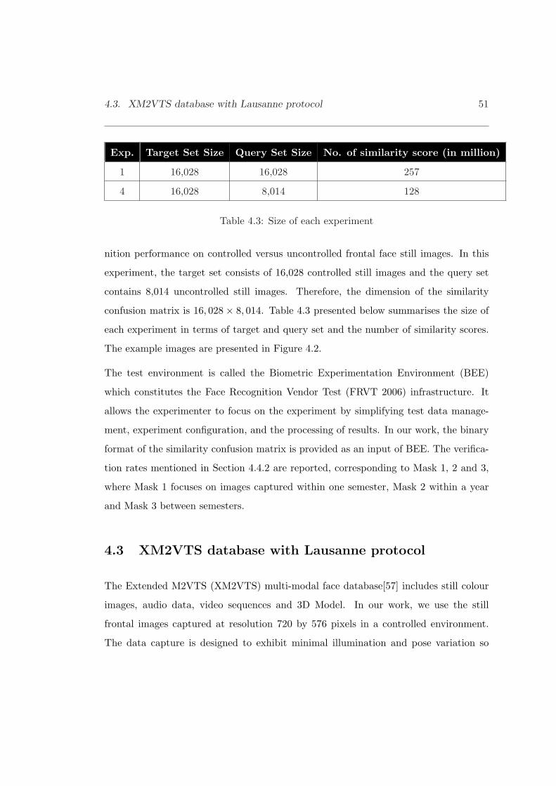
4.3. XM2VTS database with Lausanne protocol 51
Exp. Target Set Size Query Set Size No. of similarity score (in million)
1 16,028 16,028 257
4 16,028 8,014 128
Table 4.3: Size of each experiment
nition performance on controlled versus uncontrolled frontal face still images. In this
experiment, the target set consists of 16,028 controlled still images and the query set
contains 8,014 uncontrolled still images. Therefore, the dimension of the similarity
confusion matrix is 16, 028× 8, 014. Table 4.3 presented below summarises the size of
each experiment in terms of target and query set and the number of similarity scores.
The example images are presented in Figure 4.2.
The test environment is called the Biometric Experimentation Environment (BEE)
which constitutes the Face Recognition Vendor Test (FRVT 2006) infrastructure. It
allows the experimenter to focus on the experiment by simplifying test data manage-
ment, experiment configuration, and the processing of results. In our work, the binary
format of the similarity confusion matrix is provided as an input of BEE. The verifica-
tion rates mentioned in Section 4.4.2 are reported, corresponding to Mask 1, 2 and 3,
where Mask 1 focuses on images captured within one semester, Mask 2 within a year
and Mask 3 between semesters.
4.3 XM2VTS database with Lausanne protocol
The Extended M2VTS (XM2VTS) multi-modal face database[57] includes still colour
images, audio data, video sequences and 3D Model. In our work, we use the still
frontal images captured at resolution 720 by 576 pixels in a controlled environment.
The data capture is designed to exhibit minimal illumination and pose variation so

52 Chapter 4. Databases
(a) controlled image (b) controlled image (c) controlled image
(d) controlled image (e) controlled image (f) controlled image
(g) uncontrolled image (h) uncontrolled image (i) uncontrolled image
(j) uncontrolled image (k) uncontrolled image (l) uncontrolled image
Figure 4.2: Examples of FRGC 2.0 database images
4.3. XM2VTS database with Lausanne protocol 53
that the source of variation within the database is only due to inter-subject differences.
The database contains 2360 frontal face images of 295 subjects, captured for over 4
sessions at one month intervals. The testing for face verification is performed using
the Lausanne protocol which splits the database into training, evaluation and test
sets. There are two configurations that differ by the allocation of particular shots of
subjects into training and evaluation sets. The training set is used to construct client
models under the supervised learning approach. In Configuration I the client images
for training and evaluation are acquired from the first three sessions, while the client
images in Configuration II for training are from the first two sessions and the third
session is for the evaluation.
In addition to the standard set, XM2VTS database also contains a set of image with
varying illumination called Darkened set. Each subject has four more images with
lighting predominantly from one side (two image were lit from the left and two from
the right). These 1,080 images (270 subjects times 4 images) are used to evaluate the
system performance under changes of illumination. In the experiment with varying
illumination, the training and evaluation sets are from the well illuminated images
while the test set is replaced by the Darkened set. Therefore, the verification task in
this experiment is very difficult because the training model is acquired in the absence of
knowledge regarding the characteristics of the darkened image data. Table 4.4 provides
a summary of the number of data used for each step of the evaluation protocol and
Figure 4.3 gives some image examples.
The decision of acceptance or rejection is based on the relationship of a measurement
of similarity between the gallery and the average of client’s training images with a
threshold in our work. The threshold is selected at the equal error point, EER, at
which the false rejection rate is equal to the false acceptance rate on the evaluation set.
The definition of the false acceptance rate and the false rejection rate will be given in
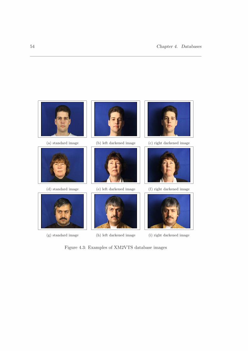
54 Chapter 4. Databases
(a) standard image (b) left darkened image (c) right darkened image
(d) standard image (e) left darkened image (f) right darkened image
(g) standard image (h) left darkened image (i) right darkened image
Figure 4.3: Examples of XM2VTS database images
4.4. Performance measures 55
DatasetLausanne Protocols
Configuration I Configuration II
No. of Training Samples 600 (3 samples ×200 client subjects)
800 (4× 200)
Evaluation Client accesses 600 (3× 200) 400 (2× 200)
Evaluation Impostor accesses 40,000 (25 imposter subjects × 8 shots ×200 client subjects)
Test Client accesses 400 (2 shots× 200 client subjects)
Test Impostor accesses 112,000 (70× 8× 200)
Test Client accesses in Darkened set 800 (4× 200)
Test Impostor accesses in Darkened set 56,000 (70× 4× 200)
Table 4.4: Number of image accesses for each dataset in the two protocols.
Section 4.4.2. The total error rate, TER, reported for the results of XM2VTS database
is defined as the sum of the false rejection rate and the false acceptance rate.
4.4 Performance measures
4.4.1 Performance measures in Face identification
The open-source publicly available evaluation framework was utilised to test and bench-
mark the performance of our methods with others. In our work, the recognition rate at
rank 1 for each probe set and two statistical measures are used to compare the perfor-
mance of the methods. These statistical measures, namely the mean recognition rate at
rank 1 and the probability of the algorithm outperforming another, are evaluated using
a set of probe images and a set of gallery images. In this statistical test, a probe-gallery

56 Chapter 4. Databases
image pair for each subject is drawn from the corresponding 12 image pairs in each
experiment involving 160 subjects and each subject has 4 images. In order to properly
infer the quality of generalisation to a larger population of subjects, a permutation
approach, generating a sampling distribution of the recognition rate for different rank
order by repeatedly computing the recognition rate from different drawn datasets in
10,000 trials, is used. The mean of the recognition rate at rank 1 defined in [8] is the
average of the recognition rate at rank 1 in total 1000 trials.
To estimate the probability of the algorithm outperforming another,P(Alg1 > Alg 2) in
rank 1 in total 1000 trials[8], the signed difference between the recognition rate of Alg1
and Alg 2 is computed in each trial. The P(Alg1 > Alg 2) is determined by summing
the probabilities of the differences greater than 0. There is a significant difference
between Alg1 and Alg 2 in terms of recognition if P(Alg1 > Alg 2) is greater than or
equal to 0.95. Otherwise, the performance of both algorithms is considered similar.
4.4.2 Performance measures in Face Verification
The verification systems make two different types of error: 1)mistaking biometric mea-
surements from two different persons to be from the same person, namely False Ac-
ceptance (FA). 2) mistaking two biometric measurements from the same person to be
from two different persons , namely False Rejection (FR). The peformance is measured
in terms of False Acceptance Rate (FAR) and False Rejection Rate (FRR), defined as:
FAR =Number of FAs
Number of imposter accesses(4.1)
FRR =Number of FRs
Number of Total True client accesses(4.2)
There is a tradeoff between FAR and FRR in every verification system, as both FAR
and FRR are a function of the threshold (T ). For a given value of the threshold (T ),

4.5. Summary 57
there is a pair of FAR(T ) and FRR(T ). They can be plotted against each other as
a curve known as Receiver Operating Characteristic (ROC) to express the behavior
of FAR and FRR. In XM2VTS experiments, the threshold is usually chosen on the
evaluation set at FAR=FRR, called Equal Error Rate (EER). It is then applied to
the test set to obtain FAR and FRR and consequently sum of both to get the Total
Error Rate (TER). By comparing the TER with other systems, our systems can be
benchmarked. On the other hand, the verification rate (i.e. 1-FRR) at 0.1% FAR is
generally used to represent the system accuracy in FRGC experiments.
4.5 Summary
In this chapter, three well-known databases are introduced for evaluating and brenching
our systems. XM2VTS and FRGC 2.0 are used for verification tasks while FERET is
used for identification tasks. The difference between the Lausanne protocol in XM2VTS
and the FRGC2.0 protocol is that the Lausanne protocol is for closed-set verification
and FRGC 2.0 is for semi-open-set experiments. In semi-open-set verification, some
subjects in the gallery or probe set never appear in the training set. However, in
the close-set verification, the subjects in gallery are in the training and evaluation
sets. In other words, the semi-open-set verification is more difficult than the closed-set
verification for the supervised learning methods. The performance of our systems using
these databases will be discussed in Chapters 5 and 6.

58 Chapter 4. Databases

Chapter 5
Advanced Local Binary Pattern
Operator
The Local Binary Pattern method has been applied in many applications, but most of
the LBP systems only work in a single image channel of a single resolution. There-
fore, the original LBP operator has the following limitations in its applications. First,
the features computed in a single-scale capturing the image structure only at a par-
ticular resolution may not necessarily be able to detect the dominant texture features,
and also they may not be robust to image translation and rotation. Second, the fea-
tures extracted in a single channel, such as gray scale image space, capture only the
monochromatic intensity information which may limit the recognition performance.
In this chapter, two novel representations, called Multi-scale LBP and Multispectral
LBP, are proposed to extend the LBP so as to provide a tool for multi-resolution and
multispectral analysis of faces. The resulting LBP methods provide input to LDA and
various classifier fusion methods for face recognition. The experimental setup is then
introduced and the results obtained on the XM2VTS, FERET and FRGC 2.0 database
59

60 Chapter 5. Advanced Local Binary Pattern Operator
discussed.
5.1 Multi-scale Local Binary Pattern (MLBP) for face
recognition
The framework of multi-scale approximation, called multi-resolution analysis, has been
developed by the computer vision, image analysis and signal processing communities
with complementary motivations from physics and biological vision. The motivation for
having a multi-scale representation of the face image comes from the basic observation
that real-world objects are composed of different structures at different scales.
In this section, a simple but powerful texture representation, called multi-scale local
binary pattern, is proposed for face recognition. This multi-resolution representation
based LBP can be obtained by varying the sample radius, R, and combining the LBP
images. It has been suggested for texture classification and the results for this applica-
tion show that its accuracy is better than that of the single scale local binary pattern
method. In general, this multiresolution LBP representation method can be realised
in two ways. First, it can be accomplished by increasing the radius of the operator.
Alternatively one can down-sample the original image with interpolation or low-pass
filtering and then apply an LBP operator of fixed radius. The difference between these
two methods is that the second one finds it difficult to extract the contrast energy in
small regions across large distance because a differential operator large enough to span
the relevant distance must trade resolution for size. Moreover, this kind of feature
has been proven to be important for face detection under different illumination con-
ditions, as explained in Section 3.1. In summary, the shortcoming of the conventional
differential operator is the confounding of the inter-lobe distance with the lobe size. In
other words, increasing the radius of the LBP operator, while keeping the size of the

5.1. Multi-scale Local Binary Pattern (MLBP) for face recognition 61
lobe constant overcomes this problem. In our system, the size of the lobe is set to be
one pixel. Thus, by sliding a set of LBP operators of different radii over an image and
combining their results, a multiresolution representation capable of capturing non-local
information can be extracted.
However, the general problem associated with the multiresolution analysis is the high
dimensionality of the representation combined with the small training sample size. It
limits the total number of LBP operators to at most 3. One of the approaches [74, 49] is
to employ a feature selection technique to minimise redundant information. We propose
another method which achieves a dimensionality reduction by feature extraction.
Certainly, extracting a multiresolution representation by using a set of LBP operators
of different radii may give an unstable result because of noise effect, but this problem
can be minimised by using aggregate statistics, such as histogram. There are several
advantages in summarising the LBP results in the form of histogram. First, the statis-
tical summary can reduce the feature dimension from the image size to the number of
histogram bins. Secondly, using histogram as a set of features is robust to image trans-
lation and rotation to a certain extent and therefore the sensitivity to mis-registration
is reduced. Finally, although the contribution to the histogram of the unstable LBP
responses due to noise is small, it can be further reduced by controlling the number of
histogram bins and /or projecting the histogram in other spaces, such as PCA. Zhao
et al. [125] have proposed to combine the local binary pattern representation with Ker-
nel Fisher Discriminant Analysis in order to improve the face verification performance
of LBP and they also mentioned that the performance of combining LBP histogram
(LBPH) with Linear Discriminant Analysis method is worse than the LBP histogram
itself. However, Shan et al. [82] and our empirical results clearly show that LBPH with
the LDA method outperforms LBPH itself. The difference between these two systems
is the use of similarity measure in which Zhao’s measure is a Euclidean metric and ours

62 Chapter 5. Advanced Local Binary Pattern Operator
is a normalised correlation. As Kittler et al. [38] have shown, the normalised correlation
can achieve better performance in the LDA space.
5.1.1 Our Face Descriptor for multiresolution analysis
In our approach, we combine the multi-scale local binary pattern representation with
Linear Discrminant Analysis, LDA. Local binary pattern operators at R scales are
first applied to a face image. This generates a grey level code for each pixel at every
resolution. The resulting LBP images, shown in Figure 5.1, are cropped to the same size
and divided into non-overlapping sub-regions, M0, M1,..MJ−1. The regional pattern
histogram for each scale is computed based on Equ (5.1)
hP,r,j(i) =∑
x′,y′∈Mj
B(LBPP,r(x′, y′) = i) | i ∈ [0, L− 1], r ∈ [1, R], j ∈ [0, J − 1],
B(v)
1 when v is true
0 otherwise(5.1)
B(v) is a Boolean indicator. The set of histograms computed at different scales for
each region, Mj , provides regional information. L is the number of histogram bins. By
concatenating these histograms into a single vector, we obtain the final multiresolution
regional face descriptor presented in Equ(5.2)
fj = [hP,1,j ,hP,2,j , · · · ,hP,R,j ] (5.2)
This regional facial descriptor can be used to measure the face similarity by fusing
the scores of local similarity of the corresponding regional histograms of the pair of
images being compared. However, by directly applying the similarity measurement to
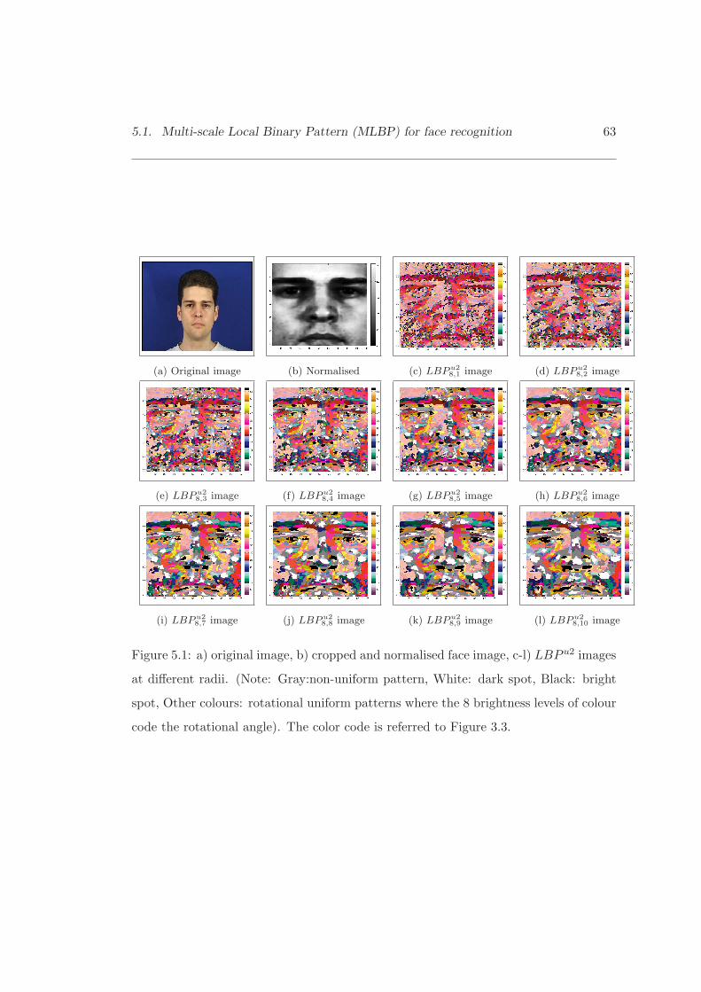
5.1. Multi-scale Local Binary Pattern (MLBP) for face recognition 63
(a) Original image (b) Normalised (c) LBP u28,1 image (d) LBP u2
8,2 image
(e) LBP u28,3 image (f) LBP u2
8,4 image (g) LBP u28,5 image (h) LBP u2
8,6 image
(i) LBP u28,7 image (j) LBP u2
8,8 image (k) LBP u28,9 image (l) LBP u2
8,10 image
Figure 5.1: a) original image, b) cropped and normalised face image, c-l) LBP u2 images
at different radii. (Note: Gray:non-uniform pattern, White: dark spot, Black: bright
spot, Other colours: rotational uniform patterns where the 8 brightness levels of colour
code the rotational angle). The color code is referred to Figure 3.3.
64 Chapter 5. Advanced Local Binary Pattern Operator
the multi-scale LBP histogram [61], the performance will be compromised. The reason
is that this histogram is of high dimensionality and contains redundant information.
By adopting the idea from [6], the dimension of the descriptor can be reduced by em-
ploying the principal component analysis (PCA) before LDA. PCA is used to extract
the statistically independent information as a prerequisite for LDA to derive discrim-
inative facial features. Thus a regional discriminative facial descriptor, dj , is defined
by projecting the histogram information, fj , into LDA space Wldaj , i.e.
dj = (Wldaj )T fj (5.3)
This discriminative descriptor, dj , gives 4 different levels of locality: 1) the local binary
patterns contributing to the histogram contain information at the pixel level, 2) the
patterns at each scale are summed over a small region to provide information at a re-
gional level, 3) the regional histograms at different scales are concatenated to produce
multiresolution information, 4) the global description of face is established by con-
catenating the regional discriminative facial descriptors. The diagram of our proposed
system is shown in Figure 5.2. Our results presented in this chapter and next chapter
show that combining Multi-scale Local Binary Pattern Histogram with LDA is more
robust in the presence of face mis-alignment and a uncontrolled environment.
5.2 Multispectral Local Binary Pattern (MSLBP) for face
recognition
Most face systems use only monochromatic intensity information, although the colour
images are commonly captured. Among most colour face recognition systems, the
colour information is coded by the response in three channels. A face recognition
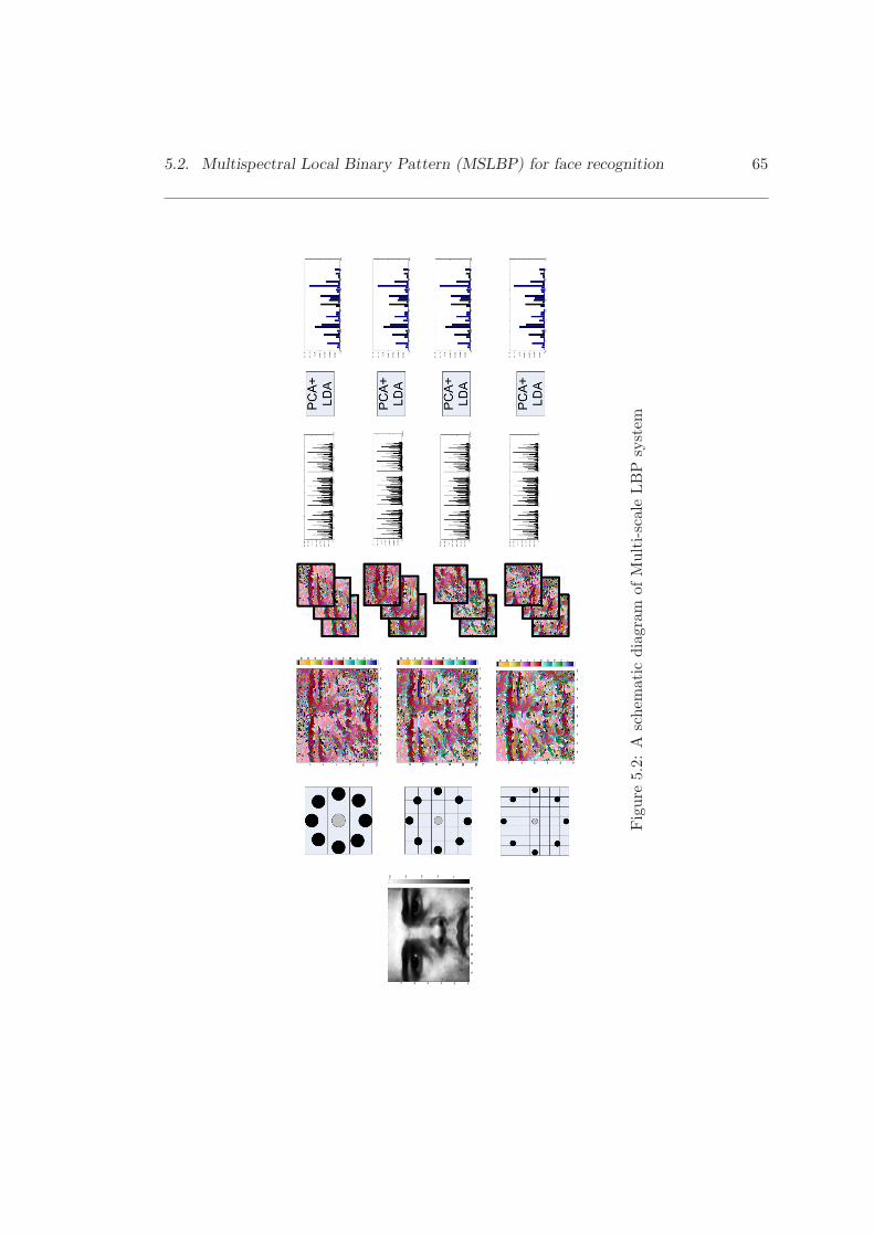
5.2. Multispectral Local Binary Pattern (MSLBP) for face recognition 65
Fig
ure
5.2:
Asc
hem
atic
diag
ram
ofM
ulti
-sca
leLB
Psy
stem
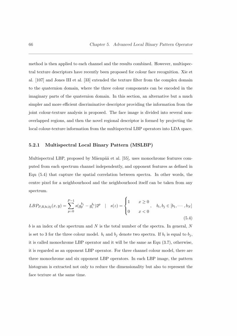
66 Chapter 5. Advanced Local Binary Pattern Operator
method is then applied to each channel and the results combined. However, multispec-
tral texture descriptors have recently been proposed for colour face recognition. Xie et
al. [107] and Jones III et al. [33] extended the texture filter from the complex domain
to the quaternion domain, where the three colour components can be encoded in the
imaginary parts of the quaternion domain. In this section, an alternative but a much
simpler and more efficient discriminative descriptor providing the information from the
joint colour-texture analysis is proposed. The face image is divided into several non-
overlapped regions, and then the novel regional descriptor is formed by projecting the
local colour-texture information from the multispectral LBP operators into LDA space.
5.2.1 Multispectral Local Binary Pattern (MSLBP)
Multispectral LBP, proposed by Maenpaa et al. [55], uses monochrome features com-
puted from each spectrum channel independently, and opponent features as defined in
Equ (5.4) that capture the spatial correlation between spectra. In other words, the
centre pixel for a neighbourhood and the neighbourhood itself can be taken from any
spectrum.
LBPP,R,bi,bj(x, y) =P−1∑
p=0
s(gbjp − gbi
c )2p | s(z) =
1 x ≥ 0
0 x < 0, bi, bj ∈ [b1, · · · , bN ]
(5.4)
b is an index of the spectrum and N is the total number of the spectra. In general, N
is set to 3 for the three colour model. bi and bj denote two spectra. If bi is equal to bj ,
it is called monochrome LBP operator and it will be the same as Equ (3.7), otherwise,
it is regarded as an opponent LBP operator. For three channel colour model, there are
three monochrome and six opponent LBP operators. In each LBP image, the pattern
histogram is extracted not only to reduce the dimensionality but also to represent the
face texture at the same time.
5.2. Multispectral Local Binary Pattern (MSLBP) for face recognition 67
The disadvantage of the multispectral LBP is that the spectra need to be normalised,
so that they are in the same range. To achieve this normalisation, the histogram
equalisation is adopted. It applies a non-linear transfer function to re-assign the input
pixel value such that the image histogram becomes as uniform as possible in each colour
spectrum.
5.2.2 Our Face Descriptor for multispectral analysis
In our approach, Linear Discrminant Analysis, LDA is combined with the multispectral
local binary pattern representation. Nine multispectral local binary pattern operators
are first applied to a face image. This generates a grey level code for each pixel in
each channel of the multispectral representation. The resulting LBP images, shown
in Figure 5.3, are divided into non-overlapping sub-regions, M0, M1,..MK−1. The
regional pattern histogram for each scale is computed based on Equ (5.5)
hP,R,bi,bj ,k(z) =1XY
∑
x′,y′∈Mk
B(LBPP,R,bi,bj (x′, y′) = z) | z ∈ [0, L− 1], x′ ∈ [0, X − 1],
y′ ∈ [0, Y − 1], r ∈ [1, R], k ∈ [0,K − 1]
B(v)
1 when v is true
0 otherwise(5.5)
where B(v) is a Boolean indicator. The set of histograms computed at different scales
for the region, Mk, provides regional information. L is the number of histogram bins.
By concatenating these histograms into a single histogram, we obtain the final multi-

68 Chapter 5. Advanced Local Binary Pattern Operator
spectral regional face descriptor presented in Equ(5.6)
fk =[hP,R,b1,b1,k,hP,R,b1,bj ,k, · · · ,hP,R,b1,bN ,k
hP,R,bj ,b1,k,hP,R,bj ,bj ,k, · · · ,hP,R,bj ,bN ,k
hP,R,bN ,b1,k,hP,R,bN ,bj ,k, · · · ,hP,R,bN ,bN ,k]
(5.6)
This regional facial descriptor can be used to measure the face similarity by fusing the
scores of the similarity between all the regional histograms. However, by directly apply-
ing the similarity measurement to the multispectral LBP histogram, the performance
will be compromised. Therefore, the histogram information, fk is projected into the
LDA space, Wldak using Equ (5.3) to obtain a regional discriminative facial descriptor,
dk.
5.3 Regional Similarity Measurement
To measure the similarity of the regional histograms of a pair of images I and I′ , there
are a number of criteria that can be applied. We have investigated four measures, which
include chi-squared, log-likelihood ratio, histogram intersection and Jensen-Shannon
divergence tests. In the following Simj denotes the histogram similarity of j-th region
of the two images.
- Chi-square criterion:
Simj(I, I′) = −∑
i
(fj(i)− f ′j(i))2
fj(i) + f ′j(i)(5.7)
where i is a bin index of the histogram.
- Histogram intersection:
Simj(I, I′) =∑
i
min(fj(i), f ′j(i)) (5.8)
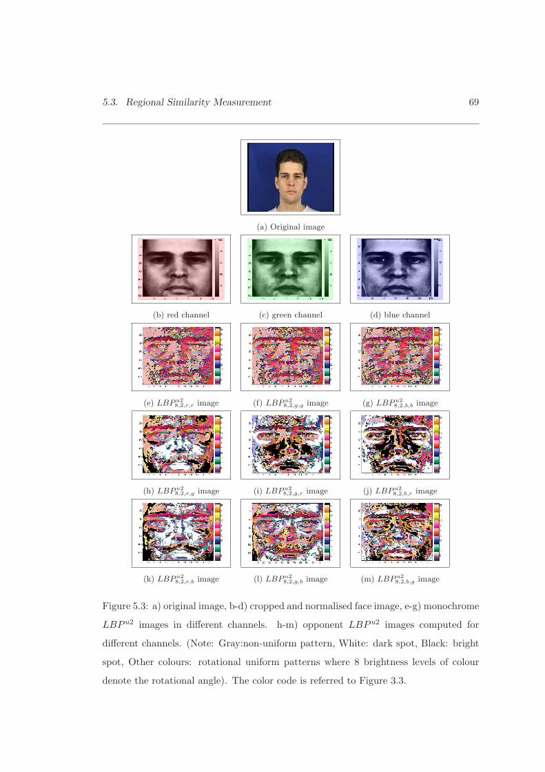
5.3. Regional Similarity Measurement 69
(a) Original image
(b) red channel (c) green channel (d) blue channel
(e) LBP u28,2,r,r image (f) LBP u2
8,2,g,g image (g) LBP u28,2,b,b image
(h) LBP u28,2,r,g image (i) LBP u2
8,2,g,r image (j) LBP u28,2,b,r image
(k) LBP u28,2,r,b image (l) LBP u2
8,2,g,b image (m) LBP u28,2,b,g image
Figure 5.3: a) original image, b-d) cropped and normalised face image, e-g) monochrome
LBP u2 images in different channels. h-m) opponent LBP u2 images computed for
different channels. (Note: Gray:non-uniform pattern, White: dark spot, Black: bright
spot, Other colours: rotational uniform patterns where 8 brightness levels of colour
denote the rotational angle). The color code is referred to Figure 3.3.
70 Chapter 5. Advanced Local Binary Pattern Operator
Since fj and f ′j are probability distributions, the bound of histogram intersection
is between 0 and 1.
- Log-likelihood ratio(Kullback-Leibler divergence):
Simj(I, I′) = DKL(fj ||f ′j) = −∑
i
fj(i) log(f ′j(i)) (5.9)
According to the log-likelihood ratio defined in [61], this metric is equivalent
to Kullback-Leibler divergence (KLD). However, KLD is unstable because it is
undefined if f ′j(i)=0 and most importantly KLD is an asymmetric measure, which
means that DKL(fj ||f ′j) is not equal toDKL(f ′j ||fj). Therefore, we propose Jensen-
Shannon divergence and the results proved that this symmetric measure was
clearly superior to KLD
- Jensen-Shannon divergence:
Simj(I, I′) = −∑
i
[fj(i) log(fj(i)) + f ′j(i) log(f ′j(i))− 2tj(i) log(tj(i))]
| tj = 0.5× (fj + f ′j)
(5.10)
After projecting the regional histogram into LDA space, the resulting feature vector is
not a probability distribution and therefore the above measurements cannot be applied.
Thus, for the feature vector in the projected space, the regional similarity measurement
is obtained by taking the normalised correlation between the regional discriminative
descriptor dj of the gallery image, and probe d′j image respectively which is presented
below.
Simj(I, I′) =djd′j
‖dj‖‖d′j‖(5.11)

5.4. Classifier Fusion 71
5.4 Classifier Fusion
In this chapter, unsupervised and supervised classifier fusion methods are also studied.
For the unsupervised method, the sum rule is proposed below.
Sim(I, I′) =J−1∑
j=0
Simj(I, I′) (5.12)
This method sums the scores of the regional classifier as the similarity measurement
of the pair of images. In contrast to the supervised methods, it is direct and fast,
but the performance is not the best. For supervised methods, both generative and
discriminative models have been studied. The classifier fusion in the supervised ap-
proach is considered as the binary classification problem in which the fusion classifier,
f , is trained using the observed regional classifier scores, v, shown below, to give the
similarity measurement between the probe and gallery images presented in Equ (5.13).
Sim(I, I′) = f(v, θ) | v = [Sim0(I, I′), Sim1(I, I′), · · · , SimJ−1(I, I′)]T (5.13)
and θ denotes the model parameters. Two types of samples, called positive and negative
sets are extracted from the evaluation samples for training. The positive set, VC =
{vi}NCi=1 , contains the similarity measurements between the elements of the training set
and the client samples in the evaluation set. The negative set, VI = {vi}NIi=1, contains
similarity measurements between the elements of the training set and the imposter
samples in the evaluation set. NC is the total number client samples multiplied by the
number of the gallery templates for each client and NI is the total number of imposter
samples multiplied by the number of the gallery templates for each client. Because the
FRGC 2.0 database contains no evaluation set, the positive and negative sets are only
obtained from the training set.

72 Chapter 5. Advanced Local Binary Pattern Operator
5.4.1 Generative Model
The Gaussian Mixture Model (GMM) is proposed and tested as a generative model.
The similarity measurement of the generative approach is log-likelihood ratio between
the client and imposter models are defined in Equ (5.14).
Sim(I, I′) = logP (v|ϕC)− logP (v|ϕI) (5.14)
where ϕC and ϕI are the parameters of the client and imposter models. P (v|ϕC) is
the likelihood of the client model and P (v|ϕI) is the likelihood of the imposter model.
In the GMM, the likelihood of a set of feature vectors is defined as
logP (v|ϕ) =G∑
i=1
tiℵ(v|µi,Σi) | ϕ = {ti, µi,Σi}Gi=1,
G∑
i=1
ti = 1 (5.15)
ℵ is a J-dimenional gaussian function with mean vector, µ, and covariance matrix, Σ,
J is the length of the vector v (the total number of non-overlapping regions). ϕ is the
learnt parameter set, G is the number of Gaussians and ti is the weight of gaussian
i. The Figueiredo-Jain method[19] is used to estimated ϕC and ϕI by providing their
corresponding training samples, VC and VI . The GMM fusion method is implement
and tested in Matlab using the GMMBAYS toolbox [62].
5.4.2 Discriminative Model
The Support Vector Machine (SVM) is proposed and tested as a discriminative model.
SVM, a binary classifier method, has been applied to face verification in [65]. It finds
the optimal linear decision surface between two hypotheses based on the concept of
structural risk minimisation. The decision surface is a weighted combination of elements
of the training samples. These elements are called support vectors. They characterise
the boundary between two classes. In the training stage, the samples are labeled as
5.5. Experiment Setup 73
{vi, ci}, where ci is +1 when vi is a positive sample, otherwise, ci is -1. The similarity
is measured using the linear SVM function presented below.
Sim(I, I′) = wTv + b | w =N∑
i=1
αicisi (5.16)
where N is the total number of support vectors, si. It can be shown that the resulting
weight vector, w, is given as a linear combination of support vectors si, with penalty,
αi, and the corresponding class label, ci. b is a bias and can be ignored. In other
words, Equ(5.16) can be viewed as a weighted sum fusion method. To evaluate the
performance of SVM, the SVM toolbox [79] is used for the XM2VTS database and
SVMperf,SVM:Joachims is used for the FRGC 2.0 database because of its large sample
size.
5.5 Experiment Setup
The goals of identification and verification systems are different. Whereas the goal of
identification is to recognise an unknown face image, verification validates a person’s
identity by comparing the captured face image with the user image template(s) stored
in the system database. However, most researchers only evaluate their algorithm either
in identification or verification scenario, which makes them very difficult to compare
with others. In order to ensure a reproducibility of the experiments and comparability
with other methods, we tested our approach on the well-known, FERET, XM2VTS
and FRGC2.0 databases using common protocols. In this experiment, face image is
extracted with the provided groundtruth eye positions and scaled to a size of 142×120
(rows× columns).
In the MLBP system, the cropped face is photometrically normalised by histogram
equalisation. In total, two parameters of the MLBP are available to optimise the system
74 Chapter 5. Advanced Local Binary Pattern Operator
performance. The first one is the LBP parameter, the circular symmetric neighbour-
hood size, P, and the method of grouping the pattern labels. A large neighbourhood
increases the length of the histogram and slows down the computation of the similarity
measure while small neighbourhood may result in information loss. We have selected
a neighbourhood P = 8 and then grouped the total number of the binary patterns
from 2P = 256 to 59 patterns according to the uniform pattern criterion mentioned in
Section 3.2.3. The second parameter is the total number of multi-scale operators. A
small number of operators not only reduces the size of the corresponding LBP images,
but also decreases the number of uniform patterns which tends to degrade the system
accuracy. In our experiments, R is set to 10, which means that ten LBP operators are
employed to represent the face image. After extracting the LBP images, they are then
cropped to the same size.
In the MSLBP system, RGB space is used for this experiment, but other colour spaces
or other aspects of the face data, such as multiresolution analysis, temporal analysis
or 3D analysis can also be considered. The cropped face in each colour channel is
photometrically normalised by histogram equalisation. In the XM2VTS database, the
evaluation set is used as a training set for the supervised classifier fusion methods. Note
that two parameters of MSLBP are available to optimise the system performance. The
first one is the LBP parameter, P , and the method of grouping LBPs. As before, we
have selected the neighbourhood of P = 8, containing 59 patterns for LBP u2. The
second parameter, the radius of LBP operators, i.e. R, is set to 2.
Having been encoded by the LBP operators, an image is partitioned into k × k non-
overlapped rectangle size regions. A large number of regions increases the computation
time as well as degrading the loss of spatial information. In this work, k is optimised
empirically. The last parameter controls the PCA transformation matrix. In general,
some of the higher order eigenvectors are removed because they do not contribute
5.6. Result and Discussions 75
to the accuracy of face recognition and the measure also saves computation. In our
experiments, the number of eigenvectors kept is determined by the requirement to
retain 98% of the energy of the signal as described in Section 2.1.5.
5.6 Result and Discussions
5.6.1 Experiments in Face Identification: FERET Database
This experiment applied the CSU standard training set to estimate the parameters of
the supervised learning methods. In this test, the recognition rate at rank1 and two
statistical measures are used to compare the performance of the methods. The measures
are the mean recognition rate with 95% confidence interval and the probability of the
algorithm outperforming another. The probability is denoted by P(Alg 1 > Alg 2)
and it is computed by permuting the gallery and probe sets, see [76] and Section 4.4.1
for details. The results with PCA, BIC and EBGM available in the CSU system as
benchmark [76] are reported in Table 5.1 for comparison.
The result of the LBP u28,2 regional histograms method with the similarity measurements
mentioned in Section 5.3, LBP u28,2 regional histograms projected on the LDA space for
normalised correlation (LBPH+LDA), and our proposed method (MLBPH+LDA+SUM)
with different k × k regions are plotted in Figure 5.4. The results show that the log-
likelihood measure (LBP KL+SUM) is clearly worse than others when k is greater
than 2. It is very difficult to say that any of the histogram similarity measures, i.e.
LBPH HI+SUM,LBPH Chi+SUM and LBPH JS+SUM, except for the log-likelihood
measure, would be the best, but the histogram intersection performs slightly better
than others in terms of the recognition rate and the computation time. Comparing the
mean recognition rate with the similarity methods in LBPH, and LBPH with LDA, it
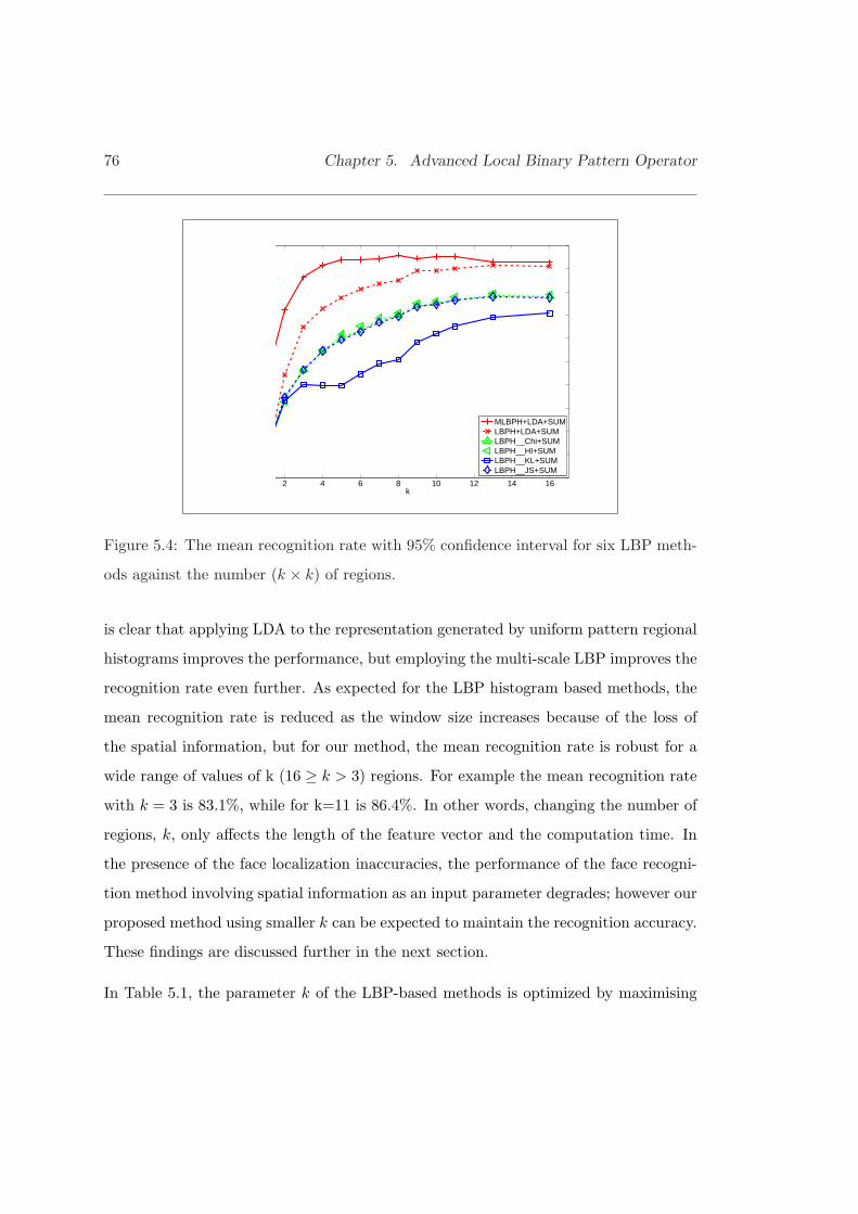
76 Chapter 5. Advanced Local Binary Pattern Operator
2 4 6 8 10 12 14 16k
MLBPH+LDA+SUMLBPH+LDA+SUMLBPH__Chi+SUMLBPH__HI+SUMLBPH__KL+SUMLBPH__JS+SUM
Figure 5.4: The mean recognition rate with 95% confidence interval for six LBP meth-
ods against the number (k × k) of regions.
is clear that applying LDA to the representation generated by uniform pattern regional
histograms improves the performance, but employing the multi-scale LBP improves the
recognition rate even further. As expected for the LBP histogram based methods, the
mean recognition rate is reduced as the window size increases because of the loss of
the spatial information, but for our method, the mean recognition rate is robust for a
wide range of values of k (16 ≥ k > 3) regions. For example the mean recognition rate
with k = 3 is 83.1%, while for k=11 is 86.4%. In other words, changing the number of
regions, k, only affects the length of the feature vector and the computation time. In
the presence of the face localization inaccuracies, the performance of the face recogni-
tion method involving spatial information as an input parameter degrades; however our
proposed method using smaller k can be expected to maintain the recognition accuracy.
These findings are discussed further in the next section.
In Table 5.1, the parameter k of the LBP-based methods is optimized by maximising
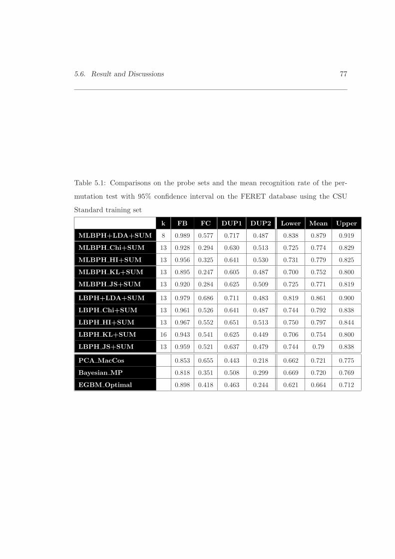
5.6. Result and Discussions 77
Table 5.1: Comparisons on the probe sets and the mean recognition rate of the per-
mutation test with 95% confidence interval on the FERET database using the CSU
Standard training set
k FB FC DUP1 DUP2 Lower Mean Upper
MLBPH+LDA+SUM 8 0.989 0.577 0.717 0.487 0.838 0.879 0.919
MLBPH Chi+SUM 13 0.928 0.294 0.630 0.513 0.725 0.774 0.829
MLBPH HI+SUM 13 0.956 0.325 0.641 0.530 0.731 0.779 0.825
MLBPH KL+SUM 13 0.895 0.247 0.605 0.487 0.700 0.752 0.800
MLBPH JS+SUM 13 0.920 0.284 0.625 0.509 0.725 0.771 0.819
LBPH+LDA+SUM 13 0.979 0.686 0.711 0.483 0.819 0.861 0.900
LBPH Chi+SUM 13 0.961 0.526 0.641 0.487 0.744 0.792 0.838
LBPH HI+SUM 13 0.967 0.552 0.651 0.513 0.750 0.797 0.844
LBPH KL+SUM 16 0.943 0.541 0.625 0.449 0.706 0.754 0.800
LBPH JS+SUM 13 0.959 0.521 0.637 0.479 0.744 0.79 0.838
PCA MacCos 0.853 0.655 0.443 0.218 0.662 0.721 0.775
Bayesian MP 0.818 0.351 0.508 0.299 0.669 0.720 0.769
EGBM Optimal 0.898 0.418 0.463 0.244 0.621 0.664 0.712
78 Chapter 5. Advanced Local Binary Pattern Operator
the mean recognition rate. LBP with LDA based methods clearly outperform the others
in all statistical tests and all probe sets except for DUP2. The reason is that there is no
training sample for DUP2 set, which is shown in Table 4.2. Comparing MLBP and LBP
both with LDA, the accuracy is not significantly different, but MLBPH+LDA+SUM is
slightly better as P(MLBPH+LDA+SUM>LBPH+LDA+SUM)=0.7830. The results
of the MLBP methods on the FC set are between 25 and 58%. One of the reasons
for having the bad performance of the MLBP methods on the FC set is that the
dimensionality of the face descriptor fj in MLBP is high, and the second is the way
the patterns are grouped to form a histogram. Lastly, face image containing cast and
attached shadows is not smooth and the key advantage of LBP, i.e. invariance to any
montonic transformation, cannot be exploited. Nevertheless, some solutions will be
mentioned in the next chapter.
Robustness to face localization error
A generic face recognition system first localizes and segments a face image from the
background before recognizing it. However, a perfect face localization method is very
difficult to achieve, and therefore a face recognition method capable of working well
in the presence of localization errors is highly desired. In order to evaluate the effect
of face localization error on the recognition rate our method achieved on the FERET
database comparatively, PCA MachCosine, LBPH+LDA+SUM and LBPH Chi+SUM
face recognition methods have also been implemented. The training images and the
gallery images in the FA set, are registered using the groundtruth eye coordinates
but the probe sets (FB, FC, Dup 1 and 2) are registered using simulated eye coordi-
nates. There are two tests in this experiment. The first test extended from Ahonen’s
experiment[2] is to simulate the translation and occlusion effects where the simulated
eye coordinates are the groundtruth eye location displaced by a random vector pertur-

5.6. Result and Discussions 79
bation (δX, δY ).
Nevertheless, this test does not realistically represent localisation error incurred by the
detection algorithm as the error in the left and right eye locations should be statistically
independent. This error causes the translation, rotation, occlusion and scale errors in
the normalised face image making the recognition problem more difficult. In order to
simulate these effects, left and right eye coordinates in the second test are computed
by adding different random vectors (δXeyeL, δYeyeL, δXeyeR, δYeyeR) of disturbances to
the groundtruth eye locations. These vectors are uncorrelated and normally distributed
with a zero mean and standard deviation, σ, from 0 to 10. For LBP based methods, a
large region size parameter, k=3, and a small region size, k=10, are tested. Moreover,
in the second test, face images are cropped to 142 × 120 pixels, while in the first test
the size of face image is 150× 130 pixels.
The mean recognition rates of LBP based methods using the respective values of param-
eter k, with PCA MachCosine and Euclidean distance against the standard deviation
of the simulated localization error are plotted in Figure 5.5a and 5.5b. As expected,
the recognition rates of all methods in the second test are worse than those in the first
test. However, the recognition rates of local region based methods clearly outperform
those of the PCA methods. Projecting LBP histograms on LDA spaces provides better
recognition rate than the error achieved in the original histogram space, in spite of the
localization error. Also, for the local region based histogram methods, the larger region
size the better the recognition rate as the localization error increases. Most importantly,
in the presence of localization error, the recognition rate of MLBPH+LDA+SUM using
a larger window size is more robust than for the other methods. The main reason for the
superior performance is the histogram combination approach and the multiresolution
representation.
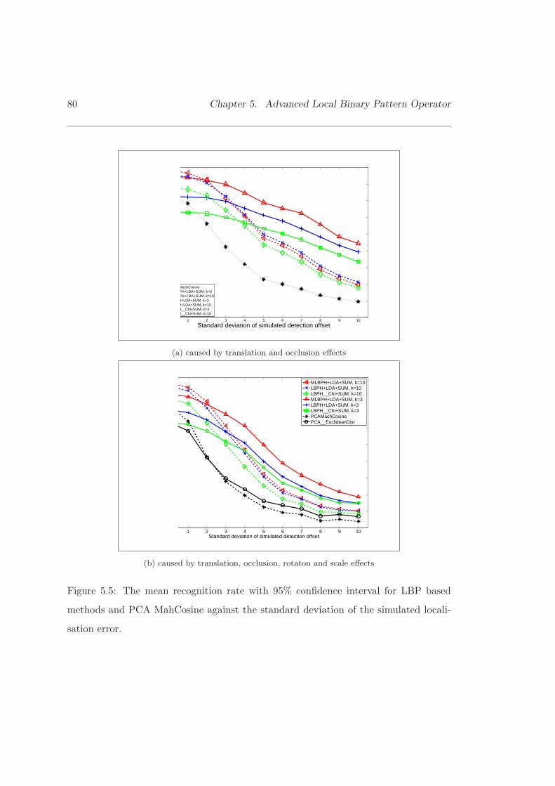
80 Chapter 5. Advanced Local Binary Pattern Operator
1 2 3 4 5 6 7 8 9 10
Standard deviation of simulated detection offset
PCAMachCosineMLBPH+LDA+SUM, k=3MLBPH+LDA+SUM, k=10LBPH+LDA+SUM, k=3LBPH+LDA+SUM, k=10LBPH__Chi+SUM, k=3LBPH__Chi+SUM, k=10
(a) caused by translation and occlusion effects
1 2 3 4 5 6 7 8 9 10Standard deviation of simulated detection offset
MLBPH+LDA+SUM, k=10LBPH+LDA+SUM, k=10LBPH__Chi+SUM, k=10MLBPH+LDA+SUM, k=3LBPH+LDA+SUM, k=3LBPH__Chi+SUM, k=3PCAMachCosinePCA__EuclideanDist
(b) caused by translation, occlusion, rotaton and scale effects
Figure 5.5: The mean recognition rate with 95% confidence interval for LBP based
methods and PCA MahCosine against the standard deviation of the simulated locali-
sation error.
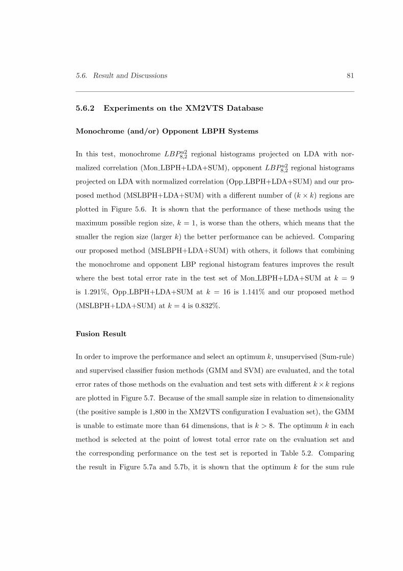
5.6. Result and Discussions 81
5.6.2 Experiments on the XM2VTS Database
Monochrome (and/or) Opponent LBPH Systems
In this test, monochrome LBP u28,2 regional histograms projected on LDA with nor-
malized correlation (Mon LBPH+LDA+SUM), opponent LBP u28,2 regional histograms
projected on LDA with normalized correlation (Opp LBPH+LDA+SUM) and our pro-
posed method (MSLBPH+LDA+SUM) with a different number of (k × k) regions are
plotted in Figure 5.6. It is shown that the performance of these methods using the
maximum possible region size, k = 1, is worse than the others, which means that the
smaller the region size (larger k) the better performance can be achieved. Comparing
our proposed method (MSLBPH+LDA+SUM) with others, it follows that combining
the monochrome and opponent LBP regional histogram features improves the result
where the best total error rate in the test set of Mon LBPH+LDA+SUM at k = 9
is 1.291%, Opp LBPH+LDA+SUM at k = 16 is 1.141% and our proposed method
(MSLBPH+LDA+SUM) at k = 4 is 0.832%.
Fusion Result
In order to improve the performance and select an optimum k, unsupervised (Sum-rule)
and supervised classifier fusion methods (GMM and SVM) are evaluated, and the total
error rates of those methods on the evaluation and test sets with different k×k regions
are plotted in Figure 5.7. Because of the small sample size in relation to dimensionality
(the positive sample is 1,800 in the XM2VTS configuration I evaluation set), the GMM
is unable to estimate more than 64 dimensions, that is k > 8. The optimum k in each
method is selected at the point of lowest total error rate on the evaluation set and
the corresponding performance on the test set is reported in Table 5.2. Comparing
the result in Figure 5.7a and 5.7b, it is shown that the optimum k for the sum rule
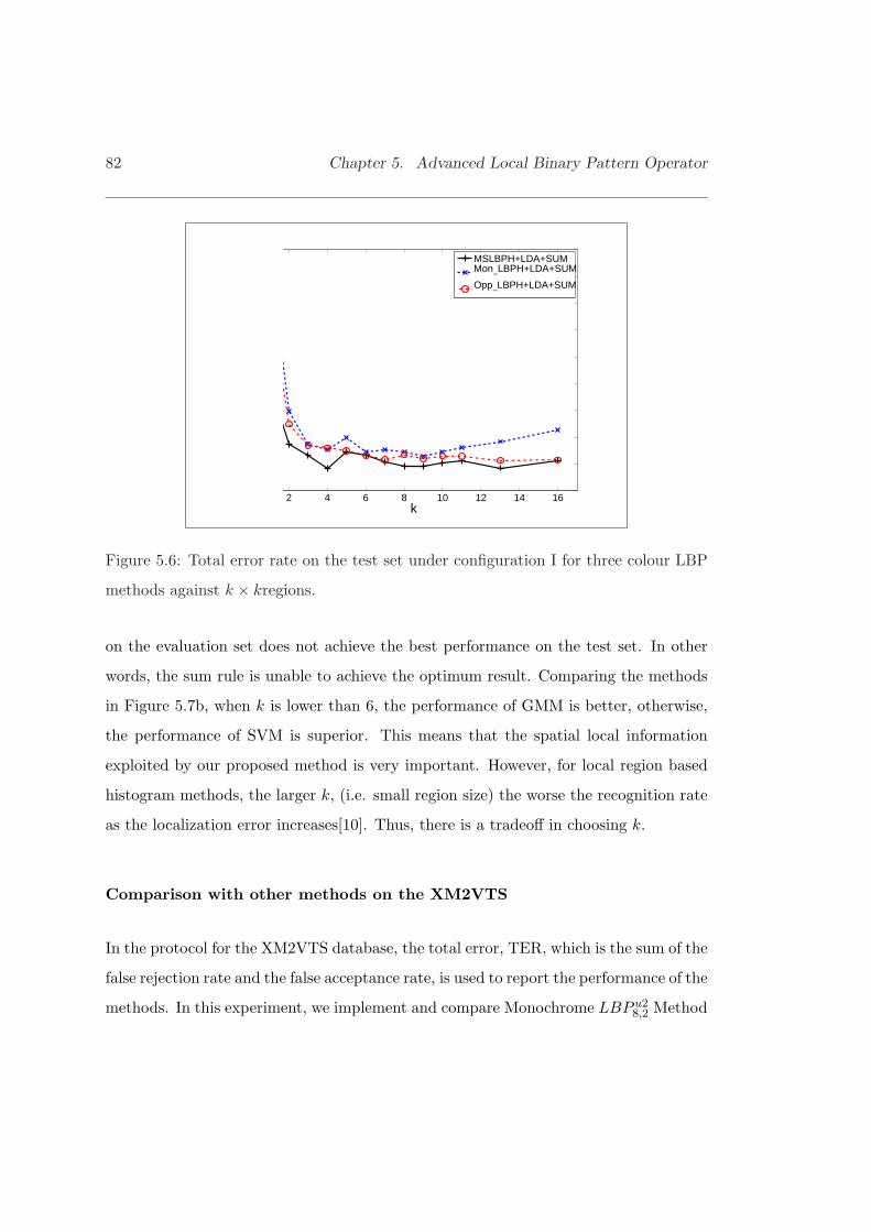
82 Chapter 5. Advanced Local Binary Pattern Operator
2 4 6 8 10 12 14 16k
MSLBPH+LDA+SUMMon
−LBPH+LDA+SUM
Opp−LBPH+LDA+SUM
Figure 5.6: Total error rate on the test set under configuration I for three colour LBP
methods against k × kregions.
on the evaluation set does not achieve the best performance on the test set. In other
words, the sum rule is unable to achieve the optimum result. Comparing the methods
in Figure 5.7b, when k is lower than 6, the performance of GMM is better, otherwise,
the performance of SVM is superior. This means that the spatial local information
exploited by our proposed method is very important. However, for local region based
histogram methods, the larger k, (i.e. small region size) the worse the recognition rate
as the localization error increases[10]. Thus, there is a tradeoff in choosing k.
Comparison with other methods on the XM2VTS
In the protocol for the XM2VTS database, the total error, TER, which is the sum of the
false rejection rate and the false acceptance rate, is used to report the performance of the
methods. In this experiment, we implement and compare Monochrome LBP u28,2 Method
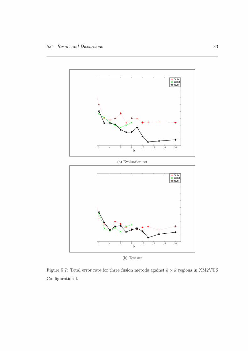
5.6. Result and Discussions 83
2 4 6 8 10 12 14 16
k
SUMGMMSVM
(a) Evaluation set
2 4 6 8 10 12 14 16k
SUMGMMSVM
(b) Test set
Figure 5.7: Total error rate for three fusion metods against k × k regions in XM2VTS
Configuration I.
84 Chapter 5. Advanced Local Binary Pattern Operator
(Mon LBPH+LDA+SUM), Opponent LBP u28,2 Method (Opp LBPH+LDA+SUM), and
our proposed approach (MSLBPH, MLBPH and LBPH+LDA) with different fusion
methods and different histogram similarity methods mentioned in Section 5.3 together
with the Adaboost classifier for LBPH [120] (LBPH+Adaboost). Rodriguez [75] found
that the total error rate of LBPH-Adaboost giving 7.88% on the test set, is worse than
that of LBPH Chi+SUM, namely 6.8%. Nevertheless, we found that the error rate
of LBPH-Adaboost can be reduced to 5.263% if 300 regional histograms (features) are
used. Table 5.2 reports the comparative results of the above mentioned methods, as well
as of the Rodriguez methods [75, 26], and the performance of the best ICPR2000[58],
the best AVBPA2003[58] and the best ICB2006[58] algorithms using the Lausanne
protocol Configuration I and II. The optimum k of those mentioned LBP mehtods is
selected at the lowest total error rate on the evaluation set. Figure 5.8 is the total error
rate for some of the LBP methods with different k parameters on the test set under
Configuration I. Figure 5.9 reports the ROC curves for some of the LBP methods, with
their corresponding optimised k×k regions, achieved on the test set under Configuration
I.
The difference between MLBPH and MSLBPH is that MLBPH is a regional multireso-
lution texture descriptor and MSLBPH is a regional colour texture descriptor capturing
texture information in each spectrum and in cross-spectra. In this experiement, the to-
tal error rate delivered by MSLBPH methods is better than that achieved by MLBPH
methods, as shown in Table 5.2, Figure 5.8 and 5.9. These results suggest that the
colour texture and/or cross-spectrum information is essential for face recognition to
achieve high accuracy. Comparing the fusion results shown in Figure 5.8, the total
error rates produced by the Support vector machine (SVM) method are lower than
those of the Sum rule especially k ≥ 11. In other words, the spatial local information
exploited by our proposed methods is very important.
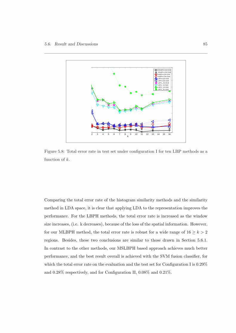
5.6. Result and Discussions 85
2 3 4 5 6 7 8 9 10 11 12 13 14 15 16k
MSLBPH+LDA+SVM
MSLBPH+LDA+SUM
MLBPH+LDA+SVM
MLBPH+LDA+SUM
LBPH+LDA+SVM
LBPH+LDA+SUM
LBPH__Chi+SUM
LBPH__HI+SUM
LBPH__JS+SUM
LBPH__KL+SUM
Figure 5.8: Total error rate in test set under configuration I for ten LBP methods as a
function of k.
Comparing the total error rate of the histogram similarity methods and the similarity
method in LDA space, it is clear that applying LDA to the representation improves the
performance. For the LBPH methods, the total error rate is increased as the window
size increases, (i.e. k decreases), because of the loss of the spatial information. However,
for our MLBPH method, the total error rate is robust for a wide range of 16 ≥ k > 2
regions. Besides, these two conclusions are similar to those drawn in Section 5.6.1.
In contrast to the other methods, our MSLBPH based approach achieves much better
performance, and the best result overall is achieved with the SVM fusion classifier, for
which the total error rate on the evaluation and the test set for Configuration I is 0.29%
and 0.28% respectively, and for Configuration II, 0.08% and 0.21%.
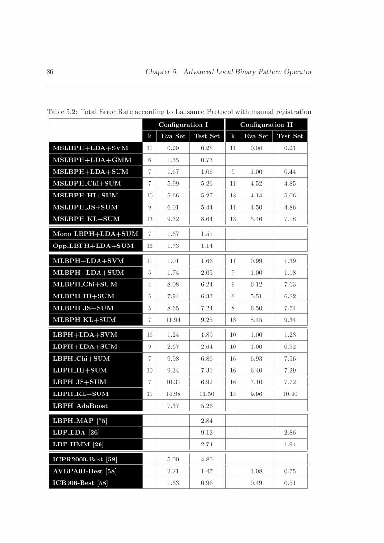
86 Chapter 5. Advanced Local Binary Pattern Operator
Table 5.2: Total Error Rate according to Lausanne Protocol with manual registration
Configuration I Configuration II
k Eva Set Test Set k Eva Set Test Set
MSLBPH+LDA+SVM 11 0.29 0.28 11 0.08 0.21
MSLBPH+LDA+GMM 6 1.35 0.73
MSLBPH+LDA+SUM 7 1.67 1.06 9 1.00 0.44
MSLBPH Chi+SUM 7 5.99 5.26 11 4.52 4.85
MSLBPH HI+SUM 10 5.66 5.27 13 4.14 5.06
MSLBPH JS+SUM 9 6.01 5.44 11 4.50 4.86
MSLBPH KL+SUM 13 9.32 8.64 13 5.46 7.18
Mono LBPH+LDA+SUM 7 1.67 1.51
Opp LBPH+LDA+SUM 16 1.73 1.14
MLBPH+LDA+SVM 11 1.01 1.66 11 0.99 1.39
MLBPH+LDA+SUM 5 1.74 2.05 7 1.00 1.18
MLBPH Chi+SUM 4 8.08 6.24 9 6.12 7.63
MLBPH HI+SUM 5 7.94 6.33 8 5.51 6.82
MLBPH JS+SUM 5 8.65 7.24 8 6.50 7.74
MLBPH KL+SUM 7 11.94 9.25 13 8.45 9.34
LBPH+LDA+SVM 16 1.24 1.89 10 1.00 1.23
LBPH+LDA+SUM 9 2.67 2.64 10 1.00 0.92
LBPH Chi+SUM 7 9.98 6.86 16 6.93 7.56
LBPH HI+SUM 10 9.34 7.31 16 6.40 7.29
LBPH JS+SUM 7 10.31 6.92 16 7.10 7.72
LBPH KL+SUM 11 14.98 11.50 13 9.96 10.40
LBPH AdaBoost 7.37 5.26
LBPH MAP [75] 2.84
LBP LDA [26] 9.12 2.86
LBP HMM [26] 2.74 1.94
ICPR2000-Best [58] 5.00 4.80
AVBPA03-Best [58] 2.21 1.47 1.08 0.75
ICB006-Best [58] 1.63 0.96 0.49 0.51
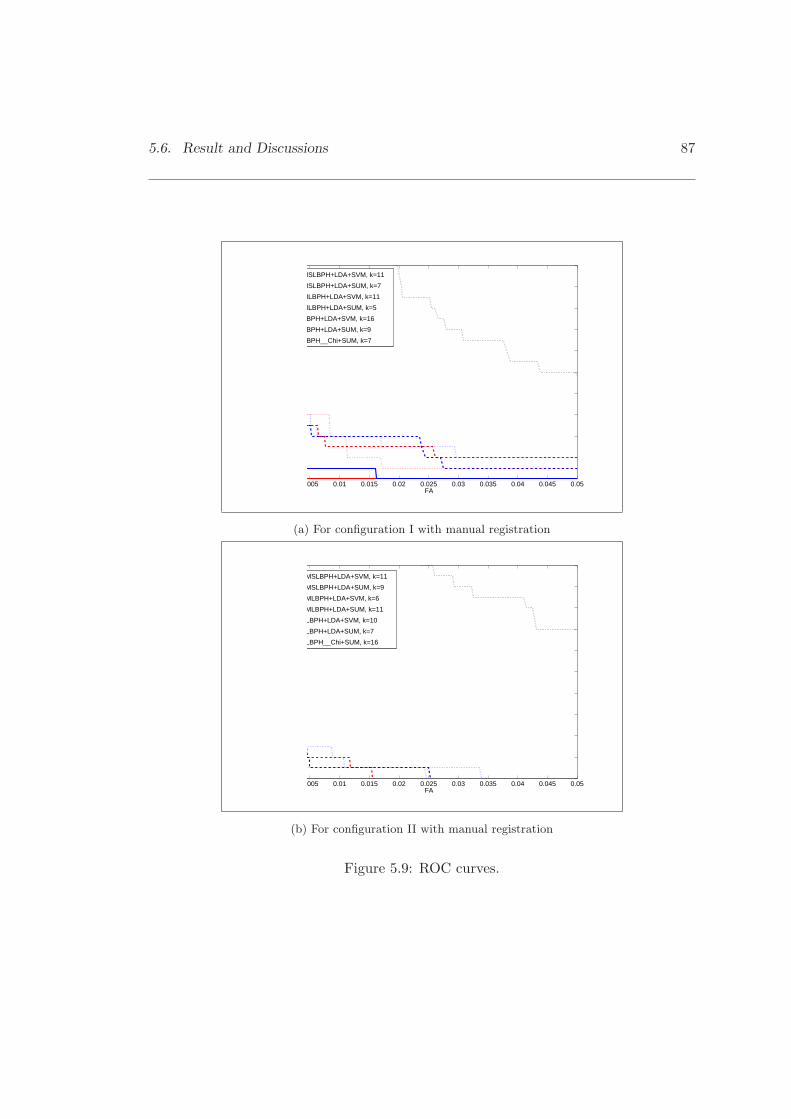
5.6. Result and Discussions 87
0.005 0.01 0.015 0.02 0.025 0.03 0.035 0.04 0.045 0.05FA
MSLBPH+LDA+SVM, k=11
MSLBPH+LDA+SUM, k=7
MLBPH+LDA+SVM, k=11
MLBPH+LDA+SUM, k=5
LBPH+LDA+SVM, k=16
LBPH+LDA+SUM, k=9
LBPH__Chi+SUM, k=7
(a) For configuration I with manual registration
0.005 0.01 0.015 0.02 0.025 0.03 0.035 0.04 0.045 0.05FA
MSLBPH+LDA+SVM, k=11
MSLBPH+LDA+SUM, k=9
MLBPH+LDA+SVM, k=6
MLBPH+LDA+SUM, k=11
LBPH+LDA+SVM, k=10
LBPH+LDA+SUM, k=7
LBPH__Chi+SUM, k=16
(b) For configuration II with manual registration
Figure 5.9: ROC curves.
88 Chapter 5. Advanced Local Binary Pattern Operator
5.6.3 Experiments on the FRGC2.0 Database
In FRGC2.0, the verification rate at 0.1% false acceptance rate (FAR) achieved by our
proposed methods (MLBPH+LDA+SUM, MSLBPH+LDA+SUM and MSLBPH+LDA+SVM)
with different number of k× k regions is plotted in Figure 5.10. For the SVM method,
the verification rate is evaluated for k ≥ 6 because the performance reported in Sec-
tion 5.6.2 showed that the accuracy improves as k becomes larger. Comparing with
the MLBPH and MSLBPH method, the smaller the region size, (larger k), the bet-
ter the MSLBPH performance. Moreover, comparing the fusion methods, the per-
formance of SVM is better than that of the Sum-rule. These two observations are
consistent with the results discussed in Section 5.6.2. Table 5.3 reports the com-
parative results of the above methods together with the Multi-scale block LBP his-
togram (MBLBPH)+Adaboost[49], LBPH Chi[49], LBPH+AdaBoost[49] and the base-
line methods. It shows that LBPH-based methods perform much better than the
baseline. Compared to the LBPH methods, our advanced versions, such as MLBPH,
MSLBPH and MBLBPH, are superior because these descriptors capture more discrim-
inative information. The performance of the MBLBPH method is similar to MLBPH
method. The main difference between MBLBP and MLBP is that the former is based
on the computation of average values of the subregions. Therefore, MBLBP captures
the local information, but finds it difficult to extract the contrast energy in small re-
gions across large distances, while our method can capture both the local and non-local
information. The non-local information has been proved to be important for face de-
tection under different illumination conditions as has been explained in Section 3.1.
However, our proposed methods are not better than MBLBPH+AdaBoost. One of the
possible reasons is the way the LBP codes are grouped into histogram. Our proposed
method exploits the concept of uniform pattern to group binary patterns. However,
the uniform local binary patterns LBP u2, are not the main patterns to represent face
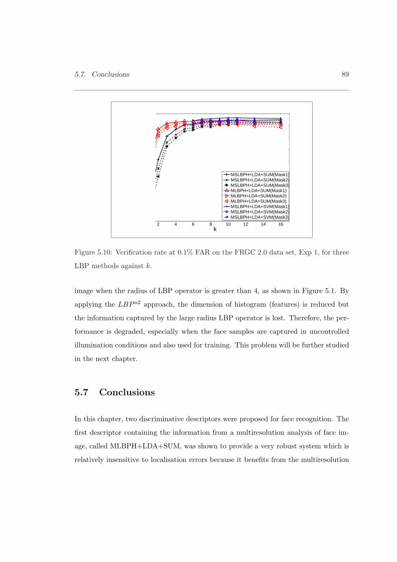
5.7. Conclusions 89
2 4 6 8 10 12 14 16k
MSLBPH+LDA+SUM(Mask1)MSLBPH+LDA+SUM(Mask2)MSLBPH+LDA+SUM(Mask3)MLBPH+LDA+SUM(Mask1)MLBPH+LDA+SUM(Mask2)MLBPH+LDA+SUM(Mask3)MSLBPH+LDA+SVM(Mask1)MSLBPH+LDA+SVM(Mask2)MSLBPH+LDA+SVM(Mask3)
Figure 5.10: Verification rate at 0.1% FAR on the FRGC 2.0 data set, Exp 1, for three
LBP methods against k.
image when the radius of LBP operator is greater than 4, as shown in Figure 5.1. By
applying the LBP u2 approach, the dimension of histogram (features) is reduced but
the information captured by the large radius LBP operator is lost. Therefore, the per-
formance is degraded, especially when the face samples are captured in uncontrolled
illumination conditions and also used for training. This problem will be further studied
in the next chapter.
5.7 Conclusions
In this chapter, two discriminative descriptors were proposed for face recognition. The
first descriptor containing the information from a multiresolution analysis of face im-
age, called MLBPH+LDA+SUM, was shown to provide a very robust system which is
relatively insensitive to localisation errors because it benefits from the multiresolution

90 Chapter 5. Advanced Local Binary Pattern Operator
Table 5.3: The verification rate in % at 0.1% FAR for different methods on FRGC 2.0
Experiment 1
k Mask1 Mask2 Mask3
MSLBPH+LDA+SVM 11 96.70 94.93 93.45
MSLBPH+LDA+SUM 16 94.82 92.85 91.79
MLBPH+LDA+SUM 7 94.73 93.21 93.76
MBLBPH+AdaBoost[49] 98.07 97.04 96.05
LBPH Chi+SUM[49] 84.17 80.35 76.67
LBPH Adaboost[49] 82.72 78.65 74.78
BaseLine PCA 74.76 70.53 66.05
information captured from the regional histogram. The system has been implemented
to support face identification and verification using the FERET, XM2VTS and FRGC
2.0 databases, and subsequently evaluated using their standard protocols. In face iden-
tification performed on the FERET database, the experimental results achieved show
that the mean recognition rate of 88% with a 95% confidence interval, delivered by
our method outperforms other state-of-the-art contenders. In particular, our system
achieved the overall best result of 98.9% recognition rate in the experiment involving
varying facial expression probe set (FB set) while delivering comparative results to other
LBP based methods for other probe sets. The MLBPH methods have been tested in the
verification mode on the XM2VTS and FRGC 2.0 databases with manual registration.
In configuration I, our MLBPH+LDA+SVM system achieved the eighth best result,
TER= 1.66%, among the total of 28 contenders, while MLBPH+LDA+SUM system
achieved the nineth best result,TER= 2.04%. In configuration II, MLBPH+LDA+SVM
achieved the sixth best result, TER=1.13% among the total of 22 contenders and
MLBPH+LDA+SUM achieved the fourth best result, TER=0.88%. In FRGC2.0 Ex-
5.7. Conclusions 91
periment 1, MLBPH+LDA achieved the verification rate of 94.73% in Mask1, 93.21% in
Mask2 and 93.76% in Mask3 at 0.1% FAR, which clearly significantly outperforms other
traditional LBPH based methods. These results showed that MLBPH+LDA(+SVM)
method not only can be comparable with the state-of-art benchmark methods, on man-
ually annotated faces but it is also more robust in the presence of localisation errors.
The second proposed discriminative descriptor exploits the colour texture information
of the face image. The descriptor is formed by projecting the local face image ac-
quired by multispectral LBP operators, into LDA space. The overall similarity score
is obtained by fusing the similarity scores of the regional descriptors. This method
has been implemented and compared with other well known benchmarks in the face
verification using the XM2VTS and FRGC 2.0 databases. In XM2VTS configuration I,
the experimental results showed that MSLBPH+LDA+SVM achieved the best result,
TER =0.28%, which is three times better than the best result (i.e. TER=0.96% [58])
reported in the literature. In XM2VTS configuration II, MSLBPH+LDA+SVM also
got the best result, TER =0.21%, which is two times better than the best known result
(i.e. TER=0.51% [58]) reported in the literatures. These results clearly show that
MSLBPH+LDA+SVM outperforms other state-of-art contenders. The proposed sys-
tem was also tested on the FRGC2.0 database. The proposed method in the verification
measured at 0.1% FAR, outperformed all other methods except the MBLBP+Adaboost
method.
Although MBLBPH is similar to MLBPH, our proposed methods are not better than
MBLBPH+AdaBoost. One of the possible reasons is the way we group the LBP codes
into histogram. Our proposed method focuses on uniform patterns as a basis of binary
patterns grouping. However, the uniform local binary patterns LBP u2, are not the
dominant patterns to represent face image when the radius of LBP operator is greater
than 4, as shown in Figure 5.1. By applying the LBP u2 approach, the dimension of

92 Chapter 5. Advanced Local Binary Pattern Operator
histogram (feature) is reduced but the information conveyed by the large radius of the
LBP operator is lost. Therefore, the performance is degraded, especially when the face
samples captured in uncontrolled illumination conditions are also used for training.
This problem will be further studied in the next chapter.
Chapter 6
A Comparison of Photometric
Normalisation Methods
Our proposed systems have comparable performance with the state-of-art benchmark
methods as demonstrated in Chapter 5. However, there still remain many problems to
be tackled for reliable face recognition in an unconstrained environment. Illumination
is known to be the one of the most significant problems. For example, ambient lighting
varies greatly everyday, as well as between indoor and outdoor environments. Moreover,
directed light source may over-saturate a part of face image and make another part being
invisible because of cast and attached shadows. Therefore, photometric normalisation
is important for face recognition, even if illumination robust features, such as Gabor or
LBP, are used for face representation as the assumption behind the invariance property
of this operator rarely holds (e.g. the function characterising illumination changes being
monotonic.) Photometric normalisation converts the image to a more canonical form
in which the illumination variations are suppressed.
Recently, numerous photometric normalisation methods have been proposed. Georghi-
93

94 Chapter 6. A Comparison of Photometric Normalisation Methods
ades et al.[21] proposed a property of images called the illumination cone to generate
and recognise image under different illumination conditions. Lee et al. [42] suggested
that linear subspaces generated by images of each individual capturing under nine point
light source directions is reliable to the recognition under a wide range of light condition.
However, these methods either require certain assumptions of the lighting directions
or need a large number of the training samples, which make them to be impractical in
the real application. On the other hand, there are alternative methods which do not
need training sample and the methods studying in this chapter are belonging to these
alternatives.
In order to study the merits of photometric normalisation, five different photometric
normalisation methods have been implemented in our proposed system. These include
Homomorphic Filtering, Contrast Limited Adaptive Histogram Equalisation[128] [72],
the Preprocessing Sequence approach[93] and the Retinex approach[23]. These methods
were compared with the results obtained with no photometric normalisation. Three
databases, XM2VTS, FERET and FRGC 2.0, are used in the experiment. In the next
section, each of the photometric normalisation methods is described in detail. Then
the experimental setup is introduced and the results discussed.
6.1 Histogram Equalisation
Histogram equalisation (HE) is one of the simple and fast photometric methods. It
improves the image contrast by using the cumulative probability distribution of the
image as a mapping function, T , presented in Equ 6.1. The equalised image is obtained
by mapping each pixel in the input image with intensity level, rk, into the corresponding

6.2. Contrast Limited Adaptive Histogram Equalisation 95
pixel with intensity level, sk.
sk = T (rk) = (L− 1)k∑
j=0
nj
n| k ∈ [0, L). (6.1)
L denotes the total number of gray levels in the image, n is the total number of
image pixels and nj is the total number of image pixels at gray level j. The examples
of the equalised image presented in Figure 6.2, 6.4, 6.5, 6.8 and 6.9. clearly show
that histogram equalisation emphasises the cast and attached shadows caused by the
directed light. The reason is that those shadows only occupy a small portion of the
image where the statistics of the entire image cannot reflect these effects and therefore
the mapping function will pick up more pixels to form the darkened part.
6.2 Contrast Limited Adaptive Histogram Equalisation
In order to overcome the above problem of Histogram Equalisation, adaptive local
histogram equalisation [72] can be applied, but it may produce noise under certain
conditions and is very slow as each pixel in the resulting image is obtained by taking the
histogram equalisation mapping of a pixel in a region surrounding that pixel. Therefore,
an advanced local histogram equalisation, namely contrast Limited Adaptive histogram
equalisation (CLAHE) [72], attempts to overcome the amplification of noise and speed
up the process. In a histogram equalisation method, the contrast enhancement can be
defined as the slope of the function mapping input intensity to output intensity. In other
words, a slope of 1 means no enhancement, and higher slopes give increasingly higher
enhancement. Thus, the limiting of contrast enhancement can be taken to involve
restricting the slope of mapping function. Since the slope of the mapping function
in histogram equalisation is the height of image histogram, limiting the slope of the
mapping function is equivalent to clipping the height of the image histogram. A major
96 Chapter 6. A Comparison of Photometric Normalisation Methods
speedup is obtained by computing the desired mapping only at a sample pixels and
interpolating the mapping between the sample locations. In other words, the sample
locations at which the mapping function is computed are on grid, and the resulting
mapping at any pixel is interpolated from the sample mappings at the four surrounding
sample-grid pixels.
The CLAHE method first divides the image into non-overlapping regions. In each
region, the histogram is computed and the predefined clipping level is used to clip the
height of the histogram. Secondly, the histogram is renormalised by redistributing the
clipping pixels into bins with the contents less than the clipping limit in proportion
to their contents such that the histogram area returns to its original value. Thirdly,
the regional cumulative histogram is computed as a regional (sample-grid) mapping
function. Finally, the pixel in the resulting image is linearly interpolated from the
sample mappings at the four surrounding sample-grid pixels.
6.3 Homomorphic Filtering (HF)
Homomorphic filtering improves image contrast by taking a filter, h, to the image, I in
the log domain for directly separating luminance and reflectance. The filtered image,
I, is performed based on the following Equ 6.2.
I = eln(I)∗h (6.2)
Since the standard convolution algorithm has a quadratic computation complexity, in
order to speed up the process, the convolution is carried out in the Fourier domain,
F , as shown in Equ 6.3, because the pointwise product of the Fourier transform is
equivalent to the convolution in spatial domain
I = eF−1[F(ln(I))×H] (6.3)

6.4. Preprocessing sequence approach (PS) 97
Figure 6.1: The block diagram of the Preprocessing sequence approach.
where H is a Gaussian high-pass filter in the Fourier domain present in Equ 6.4 based
on the assumption that luminance is generally characterised by slow spatial variations,
while reflectance tends to change suddenly.
H(u, v) = 1− a× e−[u2+v2
2σ2 ] | a ∈ [0, 1] (6.4)
a is the amplitude of the filter while σ is the bandwidth of the Gaussian function. In
our work, a is set to 0.5 and σ is set to 5.5. Motivated by Short et al., the filtered
image is histogram equalised in order to improve the performance of face recognition.
6.4 Preprocessing sequence approach (PS)
Tan et.al [93] introduced a preprocessing method based on a series of steps presented
in Figure 6.1 , designing to reduce the effects of illumination variation, local shadowing
and highlights, while still keep the essential visual appearance information for use in
recognition. The strategy of this process is similar to the homomorphic filtering in the
sense of both first taking a gamma correction and then performing a filter process. In
contrast to the PS approach, the homomorphic filtering method takes an exponential
function to form the output image.
This process first applies a gamma correction, which is a nonlinear gray level transfor-
mation replacing the pixel value in I with Iγ where γ > 0. The objective of this process
is to enhance the local dynamic range of the image in dark and shadow regions, while

98 Chapter 6. A Comparison of Photometric Normalisation Methods
suppressing the bright region. In our work, γ is set to 0.2. Then the image is processed
by a band-pass filter that is the difference of Gaussian filtering shown in Equ 6.5 to
remove the influence of intensity gradients such as shading effects, while homomorphic
filtering uses the high-pass filter. The reason of choosing the band-pass filter is that
it not only suppresses low frequency information caused by illumination gradient, but
also reduces the high frequency noise due to aliasing artifacts.
DoG = (2π)−12 [σ−1
1 e−x2+y2
(2σ1)2 − σ−12 e
−x2+y2
(2σ2)2 ] (6.5)
In our work, σ1 is set to 1 and σ2 is set 2. Then, the two stage contrast equalisa-
tion presented in Equ 6.6 and Equ 6.7 is employed to further re-normalise the image
intensities and standardise the overall contrast.
J(x, y) =I(x, y)
(mean(|I(x, y)|a)) 1a
(6.6)
J(x, y) =J(x, y)
(mean(min(τ, |J(x, y)|)a))1a
(6.7)
a, set to 0.1, is used to reduces the influence of large values and τ ,set to 10, is a
threshold used to truncate large values after the first stage of normalisation. Lastly, a
hyperbolic tangent function in Equ 6.8 is applied to suppress the extreme values and
limit the pixel values in normalised image,I, to a range between −τ and τ
I(x, y) = τtanh(J(x, y)τ
) (6.8)
6.5 Retinex
The goal of the Retinex method is to decompose the image I(x, y), shown in Equ 6.9
into two components, reflectance, R(x, y), and luminance, L(x, y).
I(x, y) = L(x, y)R(x, y) (6.9)

6.5. Retinex 99
Luminance is determined by the light source position and the surface normals of face,
and reflectance is determined by the attenuation of the reflection at the object surface.
In other words, reflectance has the property of an illumination invariant. Thus, by
estimating the luminance as a low frequency component of the original image, the
reflectance can be obtained by computing the ratio of the image and the luminance
component. Jobson et al. [32] proposed a method called multiscale retinex (MSR)
which applies a set of Gaussian low pass filters to the image to estimate the luminances
in different resolutionss. The reflectance of the image is computed by summing a non-
linear transform of the ratio of the image and the luminance component in different
resolutions. More recently, Self Quotent Image (SQI) [100] has been proposed which is
similar to MSR. In contrast with MSR, SQI employs a special Gaussian kernal function
in which a portion of the kernal is plane to reduce the halo effects. In our work,
the luminance component is estimated by applying an anisotropic diffusion process to
the original image [23]. This process is implemented by minimising the following cost
function.
J(L) =∫
y
∫
xρ(x, y)(L− I)2dxdy + λ
∫
y
∫
xL2
x + L2ydxdy (6.10)
The first term forces luminance to be close to the original image, while the second term
imposes a smooth constraint. λ controls the relative importance of the two terms and
the weight, ρ(x, y), controls the anisotropic smoothing. Given the cost function in Equ
6.10, the Euler-Lagrange equation can be used to solve this optimisation problem and
the solution is presented below.
Ix,y = Lx,y + λ[1
ρN (x, y)(Lx,y − Lx,y−1) +
1ρS(x, y)
(Lx,y − Lx,y+1)
+1
ρE(x, y)(Lx,y − Lx−1,y) +
1ρW (x, y)
(Lx,y − Lx+1,y)] (6.11)
where the anisotropic diffusion coefficients, ρdirection, are defined as the reciprocal of
the Weber contrast measure, which is calculated between the pixel, a and its neighbour,
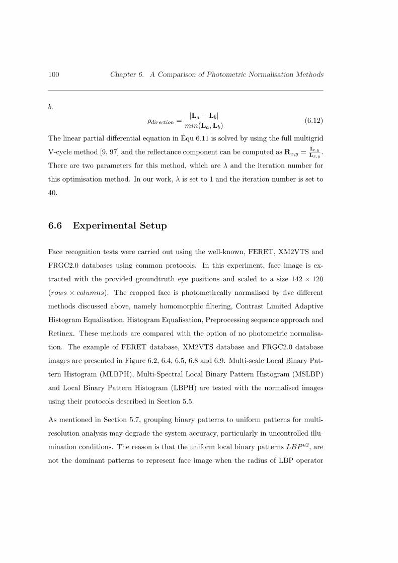
100 Chapter 6. A Comparison of Photometric Normalisation Methods
b.
ρdirection =|La − Lb|min(La,Lb)
(6.12)
The linear partial differential equation in Equ 6.11 is solved by using the full multigrid
V-cycle method [9, 97] and the reflectance component can be computed as Rx,y = Ix,y
Lx,y.
There are two parameters for this method, which are λ and the iteration number for
this optimisation method. In our work, λ is set to 1 and the iteration number is set to
40.
6.6 Experimental Setup
Face recognition tests were carried out using the well-known, FERET, XM2VTS and
FRGC2.0 databases using common protocols. In this experiment, face image is ex-
tracted with the provided groundtruth eye positions and scaled to a size 142 × 120
(rows × columns). The cropped face is photometircally normalised by five different
methods discussed above, namely homomorphic filtering, Contrast Limited Adaptive
Histogram Equalisation, Histogram Equalisation, Preprocessing sequence approach and
Retinex. These methods are compared with the option of no photometric normalisa-
tion. The example of FERET database, XM2VTS database and FRGC2.0 database
images are presented in Figure 6.2, 6.4, 6.5, 6.8 and 6.9. Multi-scale Local Binary Pat-
tern Histogram (MLBPH), Multi-Spectral Local Binary Pattern Histogram (MSLBP)
and Local Binary Pattern Histogram (LBPH) are tested with the normalised images
using their protocols described in Section 5.5.
As mentioned in Section 5.7, grouping binary patterns to uniform patterns for multi-
resolution analysis may degrade the system accuracy, particularly in uncontrolled illu-
mination conditions. The reason is that the uniform local binary patterns LBP u2, are
not the dominant patterns to represent face image when the radius of LBP operator
6.7. Result and Discussions 101
is greater than 4, as shown in Figure 5.1, and thus the system loses the information
conveyed by the large radius of the LBP operator. In order to investigate this issue, a
full LBP grouping method is used. In other words, there are 256 local binary patterns
for 3 × 3 neighbourhood LBP coding in each scale and this representation is referred
to as Multi-scale Full Local Binary Pattern Histogram (MFLBPH).
6.7 Result and Discussions
6.7.1 Experiments in Face Identification: FERET Database
Example images of the different normalisation methods are presented in Figure 6.2.
Subjectively, the image quality of Retinex and PS methods is similar. Both methods
reduce the shading effect and shadow effect, while the images presented by the PS
method give a better contrast on facial features such as mole, mouth and eyes. The
image quality of HF and HE normalised faces also appear to be similar, but our ex-
perimental results show that the performance of the HF method in different LBPH
systems is better. The image quality of CLAHE is good from the human perception
point of view because the images retain more texture information as compared with
other methods, but our results show that CLAHE is not better than the PS and retinex
methods. The reason is that the face image output by CLAHE amplifies bright regions,
such as the nose tip, chin and forehead, depending on the light direction.
In this test, the recognition rate at rank 1 and two statistical measures are used to
compare the performance of the methods. The measures are the mean recognition
rate with 95% confidence interval and the probability of the algorithm outperforming
another. The probability is denoted by P(Alg 1 > Alg 2) and it is computed by
permuting the gallery and probe sets, (see [76] and Section 4.4.1 for details). The CSU
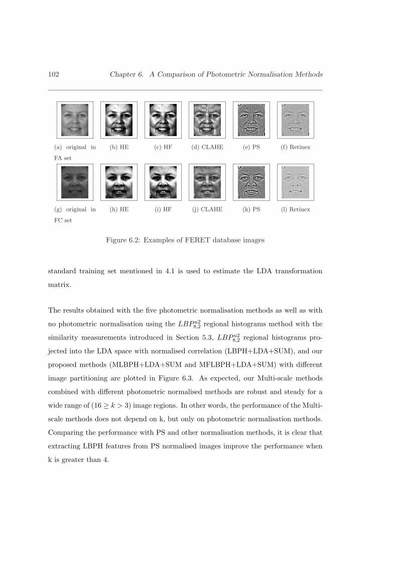
102 Chapter 6. A Comparison of Photometric Normalisation Methods
(a) original in
FA set
(b) HE (c) HF (d) CLAHE (e) PS (f) Retinex
(g) original in
FC set
(h) HE (i) HF (j) CLAHE (k) PS (l) Retinex
Figure 6.2: Examples of FERET database images
standard training set mentioned in 4.1 is used to estimate the LDA transformation
matrix.
The results obtained with the five photometric normalisation methods as well as with
no photometric normalisation using the LBP u28,2 regional histograms method with the
similarity measurements introduced in Section 5.3, LBP u28,2 regional histograms pro-
jected into the LDA space with normalised correlation (LBPH+LDA+SUM), and our
proposed methods (MLBPH+LDA+SUM and MFLBPH+LDA+SUM) with different
image partitioning are plotted in Figure 6.3. As expected, our Multi-scale methods
combined with different photometric normalised methods are robust and steady for a
wide range of (16 ≥ k > 3) image regions. In other words, the performance of the Multi-
scale methods does not depend on k, but only on photometric normalisation methods.
Comparing the performance with PS and other normalisation methods, it is clear that
extracting LBPH features from PS normalised images improve the performance when
k is greater than 4.
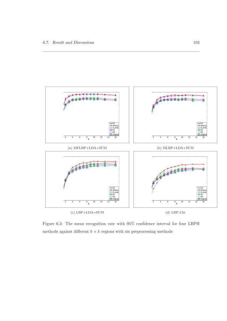
6.7. Result and Discussions 103
2 4 6 8 10 12 14 16k
PSRetinexCLAHEHFHEOriginal
(a) MFLBP+LDA+SUM
2 4 6 8 10 12 14 16k
PSRetinexCLAHEHFHEOriginal
(b) MLBP+LDA+SUM
2 4 6 8 10 12 14 16k
PSRetinexCLAHEHFHEOriginal
(c) LBP+LDA+SUM
2 4 6 8 10 12 14 16k
PSRetinexCLAHEHFHEOriginal
(d) LBP Chi
Figure 6.3: The mean recognition rate with 95% confidence interval for four LBPH
methods against different k × k regions with six preprocessing methods
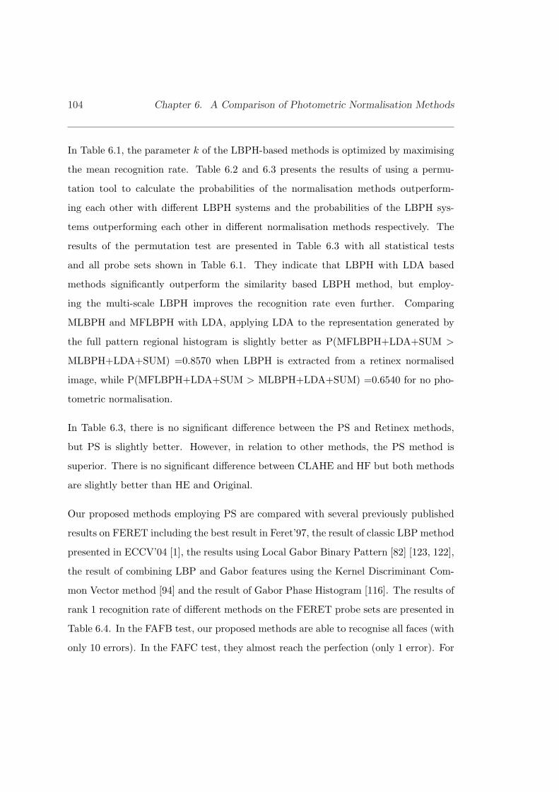
104 Chapter 6. A Comparison of Photometric Normalisation Methods
In Table 6.1, the parameter k of the LBPH-based methods is optimized by maximising
the mean recognition rate. Table 6.2 and 6.3 presents the results of using a permu-
tation tool to calculate the probabilities of the normalisation methods outperform-
ing each other with different LBPH systems and the probabilities of the LBPH sys-
tems outperforming each other in different normalisation methods respectively. The
results of the permutation test are presented in Table 6.3 with all statistical tests
and all probe sets shown in Table 6.1. They indicate that LBPH with LDA based
methods significantly outperform the similarity based LBPH method, but employ-
ing the multi-scale LBPH improves the recognition rate even further. Comparing
MLBPH and MFLBPH with LDA, applying LDA to the representation generated by
the full pattern regional histogram is slightly better as P(MFLBPH+LDA+SUM >
MLBPH+LDA+SUM) =0.8570 when LBPH is extracted from a retinex normalised
image, while P(MFLBPH+LDA+SUM > MLBPH+LDA+SUM) =0.6540 for no pho-
tometric normalisation.
In Table 6.3, there is no significant difference between the PS and Retinex methods,
but PS is slightly better. However, in relation to other methods, the PS method is
superior. There is no significant difference between CLAHE and HF but both methods
are slightly better than HE and Original.
Our proposed methods employing PS are compared with several previously published
results on FERET including the best result in Feret’97, the result of classic LBP method
presented in ECCV’04 [1], the results using Local Gabor Binary Pattern [82] [123, 122],
the result of combining LBP and Gabor features using the Kernel Discriminant Com-
mon Vector method [94] and the result of Gabor Phase Histogram [116]. The results of
rank 1 recognition rate of different methods on the FERET probe sets are presented in
Table 6.4. In the FAFB test, our proposed methods are able to recognise all faces (with
only 10 errors). In the FAFC test, they almost reach the perfection (only 1 error). For

6.7. Result and Discussions 105
Table 6.1: Comparisons of photometric normalisation methods on the probe sets and
the mean recognition rate of the permutation test with 95% confidence interval on the
FERET database using the CSU Standard training setk FB FC DUP1 DUP2 Lower Mean Upper
PS
MFLBPH+LDA+SUM 11 0.992 0.995 0.900 0.855 0.944 0.970 0.988
MLBPH+LDA+SUM 11 0.992 0.995 0.884 0.812 0.925 0.955 0.981
LBPH+LDA+SUM 11 0.985 0.990 0.846 0.786 0.888 0.926 0.956
LBPH Chi+SUM 13 0.967 0.969 0.788 0.774 0.838 0.879 0.919
Reti
nex
MFLBPH+LDA+SUM 8 0.990 1.000 0.886 0.795 0.938 0.962 0.988
MLBPH+LDA+SUM 11 0.990 0.995 0.845 0.726 0.912 0.945 0.975
LBPH+LDA+SUM 13 0.985 0.974 0.780 0.607 0.862 0.903 0.938
LBPH Chi+SUM 13 0.965 0.964 0.738 0.692 0.769 0.816 0.862
CLA
HE
MFLBPH+LDA+SUM 9 0.982 0.747 0.766 0.607 0.869 0.904 0.938
MLBPH+LDA+SUM 11 0.976 0.845 0.759 0.620 0.856 0.895 0.931
LBPH+LDA+SUM 13 0.968 0.825 0.766 0.628 0.844 0.886 0.925
LBPH Chi+SUM 13 0.951 0.742 0.704 0.637 0.775 0.819 0.862
HF
MFLBPH+LDA+SUM 11 0.987 0.820 0.763 0.581 0.869 0.905 0.938
MLBPH+LDA+SUM 11 0.985 0.773 0.748 0.556 0.862 0.897 0.931
LBPH+LDA+SUM 13 0.978 0.830 0.733 0.530 0.844 0.882 0.919
LBPH Chi+SUM 13 0.964 0.613 0.668 0.526 0.762 0.807 0.850
HE
MFLBPH+LDA+SUM 9 0.989 0.655 0.738 0.504 0.856 0.893 0.931
MLBPH+LDA+SUM 8 0.989 0.577 0.717 0.487 0.838 0.879 0.919
LBPH+LDA+SUM 13 0.979 0.686 0.711 0.483 0.819 0.861 0.900
LBPH Chi+SUM 13 0.961 0.526 0.641 0.487 0.744 0.792 0.838
Ori
gin
al MFLBPH+LDA+SUM 9 0.987 0.670 0.737 0.509 0.850 0.887 0.925
MLBPH+LDA+SUM 11 0.985 0.711 0.733 0.547 0.838 0.878 0.919
LBPH+LDA+SUM 16 0.977 0.804 0.708 0.470 0.819 0.859 0.900
LBPH Chi+SUM 16 0.962 0.588 0.643 0.487 0.744 0.789 0.838
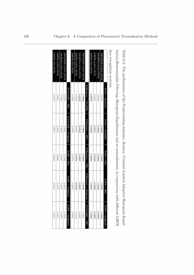
106 Chapter 6. A Comparison of Photometric Normalisation Methods
Table
6.2:T
heperform
anceofthe
Preprocessing
sequence,Retinex,C
ontrastLim
itedA
daptiveH
istogramE
qual-
isation,Hom
omorphic
Filtering,H
istogramE
qualisationand
nonorm
alisation,inconjunction
with
differentLB
PH
facerecognition
systems.P
(P
S>
Retin
ex)
P(P
S>
CLA
HE)
P(P
S>
HF)
P(P
S>
HE)
P(P
S>
Orig
inal)
MFLB
PH
+LD
A+
SU
M0.6
379
0.9
999
1.0
000
1.0
000
1.0
000
MLB
PH
+LD
A+
SU
M0.6
948
0.9
995
0.9
984
1.0
000
0.9
999
LB
PH
+LD
A+
SU
M0.8
393
0.9
721
0.9
799
0.9
989
0.9
987
LB
PH
Chi+
SU
M0.9
975
0.9
983
0.9
990
1.0
000
1.0
000
P(R
etin
ex
>C
LA
HE)
P(R
etin
ex
>H
F)
P(R
etin
ex
>H
E)
P(R
etin
ex
>O
rig
inal)
P(C
LA
HE
>H
F)
MFLB
PH
+LD
A+
SU
M0.9
993
0.9
992
0.9
999
0.9
999
0.4
014
MLB
PH
+LD
A+
SU
M0.9
955
0.9
936
0.9
997
0.9
997
0.3
697
LB
PH
+LD
A+
SU
M0.7
633
0.8
158
0.9
705
0.9
746
0.5
159
LB
PH
Chi+
SU
M0.3
933
0.5
936
0.7
978
0.8
204
0.6
927
P(C
LA
HE
>H
E)
P(C
LA
HE
>O
rig
inal)
P(H
F>
HE)
P(H
F>
Orig
inal)
P(H
E>
Orig
inal)
MFLB
PH
+LD
A+
SU
M0.6
769
0.7
891
0.7
258
0.8
374
0.5
938
MLB
PH
+LD
A+
SU
M0.7
652
0.7
982
0.8
376
0.8
840
0.4
378
LB
PH
+LD
A+
SU
M0.8
951
0.9
108
0.8
800
0.8
783
0.4
621
LB
PH
Chi+
SU
M0.9
115
0.9
272
0.8
322
0.8
412
0.4
945
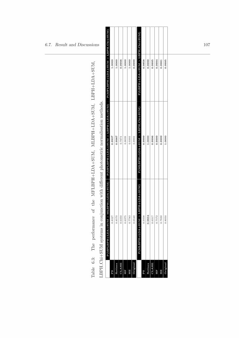
6.7. Result and Discussions 107
Tab
le6.
3:T
hepe
rfor
man
ceof
the
MFLB
PH
+LD
A+
SUM
,M
LB
PH
+LD
A+
SUM
,LB
PH
+LD
A+
SUM
,
LB
PH
Chi
+SU
Msy
stem
sin
conj
unct
ion
wit
hdi
ffere
ntph
otom
etri
cno
rmal
isat
ion
met
hods
.P
(M
FLB
PH
+LD
A+
SU
M>
MLB
PH
+LD
A+
SU
M)
P(M
FLB
PH
+LD
A+
SU
M>
LB
PH
+LD
A+
SU
M)
P(M
FLB
PH
+LD
A+
SU
M>
LB
PH
Chi+
SU
M)
PS
0.8
327
0.9
937
1.0
000
Retin
ex
0.8
570
0.9
987
1.0
000
CLA
HE
0.6
350
0.7
873
0.9
998
HF
0.6
375
0.8
639
1.0
000
HE
0.7
783
0.9
393
1.0
000
Orig
inal
0.6
540
0.8
993
0.9
999
P(M
LB
PH
+LD
A+
SU
M>
LB
PH
+LD
A+
SU
M)
P(M
LB
PH
+LD
A+
SU
M>
LB
PH
Chi+
SU
M)
P(LB
PH
+LD
A+
SU
M>
LB
PH
Chi+
SU
M)
PS
0.9
358
0.9
999
0.9
858
Retin
ex
0.9
834
1.0
000
0.9
999
CLA
HE
0.6
317
0.9
996
0.9
995
HF
0.7
572
0.9
999
0.9
994
HE
0.7
830
0.9
999
0.9
981
Orig
inal
0.8
050
1.0
000
0.9
995
108 Chapter 6. A Comparison of Photometric Normalisation Methods
Table 6.4: Comparing with the state of art methods on the standard FERET probe
sets
FB FC DUP1 DUP2
PS MFLBPH+LDA+SUM 0.992 0.995 0.900 0.855
PS MLBPH+LDA+SUM 0.992 0.995 0.884 0.812
ICPR06’ EPFDA LGBP [82] 0.996 0.990 0.920 0.889
AMFG07’ PS (LBP,Gabor)+KDCV [94] 0.98 0.98 0.90 0.85
PAA08’ ELGBP (Mag + Pha) W [123] 0.99 0.96 0.78 0.77
IJIG07’ FM LGBP [122] 0.99 0.98 0.79 0.80
IP07’ HGPP Weighted [116] 0.975 0.995 0.795 0.778
ECCV04’ LBP weighted [1] 0.97 0.79 0.66 0.64
CVPR97’ Best FERET [68] 0.96 0.82 0.59 0.52
the aging tests, DUP1 and DUP 2, our proposed methods achieved almost 90%. The
performance of our proposed methods is comparable to or better than existing the state-
of-art results. In the FAFB and Aging group tests, our PS MFLBPH+LDA+SUM is
slighly worse than EPFDA LGBP. One possible reason is the poor generalisation of the
LDA because the training set using the FERET standard contains 270 samples from
the FB set and 85 more samples from the DUP1 set.
6.7.2 Experiments on the XM2VTS Database
The XM2VTS database is used to verify the performance of face verification in a vari-
able lighting environment. Five different normalisation methods are tested on this
database with example images presented in Figure 6.4 and 6.5. By looking at these ex-
amples, it is evident that none of the methods can fully eliminate the effect of directed
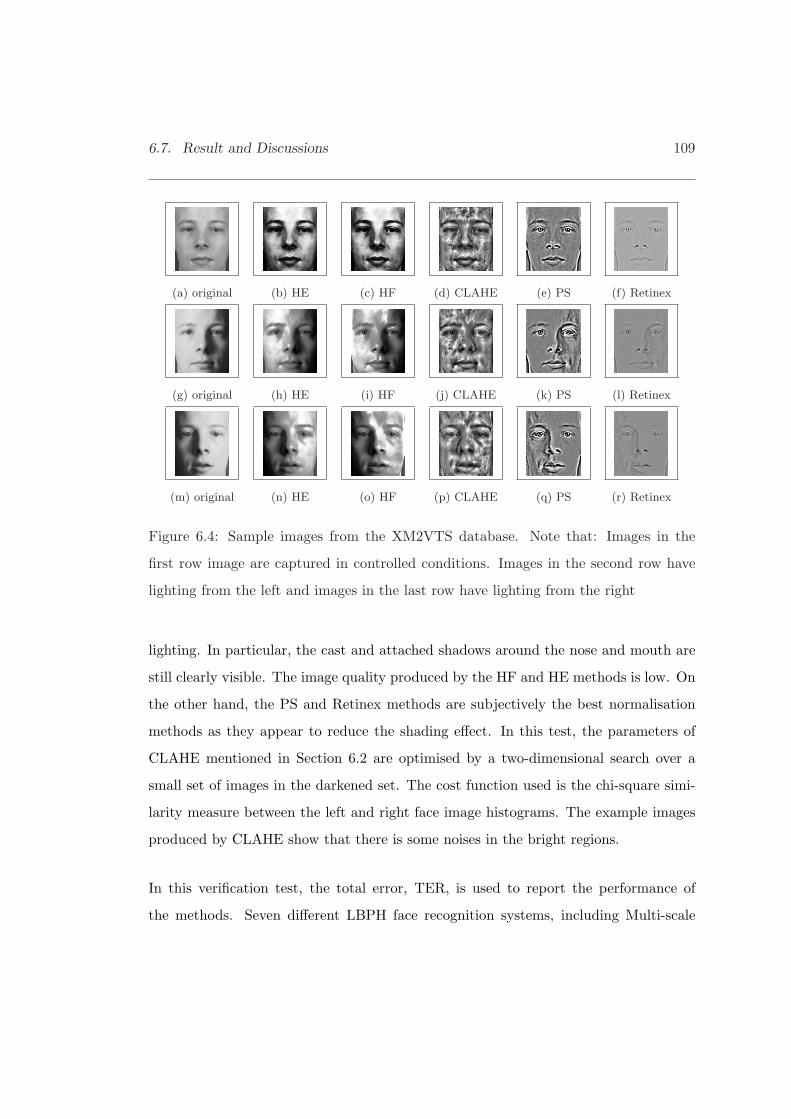
6.7. Result and Discussions 109
(a) original (b) HE (c) HF (d) CLAHE (e) PS (f) Retinex
(g) original (h) HE (i) HF (j) CLAHE (k) PS (l) Retinex
(m) original (n) HE (o) HF (p) CLAHE (q) PS (r) Retinex
Figure 6.4: Sample images from the XM2VTS database. Note that: Images in the
first row image are captured in controlled conditions. Images in the second row have
lighting from the left and images in the last row have lighting from the right
lighting. In particular, the cast and attached shadows around the nose and mouth are
still clearly visible. The image quality produced by the HF and HE methods is low. On
the other hand, the PS and Retinex methods are subjectively the best normalisation
methods as they appear to reduce the shading effect. In this test, the parameters of
CLAHE mentioned in Section 6.2 are optimised by a two-dimensional search over a
small set of images in the darkened set. The cost function used is the chi-square simi-
larity measure between the left and right face image histograms. The example images
produced by CLAHE show that there is some noises in the bright regions.
In this verification test, the total error, TER, is used to report the performance of
the methods. Seven different LBPH face recognition systems, including Multi-scale
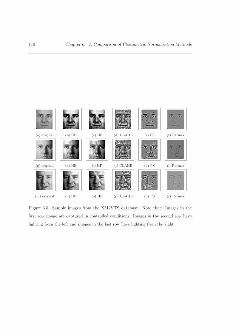
110 Chapter 6. A Comparison of Photometric Normalisation Methods
(a) original (b) HE (c) HF (d) CLAHE (e) PS (f) Retinex
(g) original (h) HE (i) HF (j) CLAHE (k) PS (l) Retinex
(m) original (n) HE (o) HF (p) CLAHE (q) PS (r) Retinex
Figure 6.5: Sample images from the XM2VTS database. Note that: Images in the
first row image are captured in controlled conditions. Images in the second row have
lighting from the left and images in the last row have lighting from the right

6.7. Result and Discussions 111
Full Local Binary Pattern Histogram LDA method (MFLBPH+LDA+SUM), Multi-
scale uniform Local Binary Pattern Histogram method (MLBPH+LDA+SUM), Multi-
spectral Local Binary Pattern Histogram method (MSLBPH+LDA+SUM) and Local
Binary Histogram (LBPH+LDA+SUM) with their corresponding SVM discriminant
function approach and Local Binary Histogram with the Chi-square similarity method
(LBPH Chi+SUM), are implemented and compared. Figures 6.6 and 6.7 present the
total error rate for some of the LBPH methods with different k parameters and different
normalisation methods on the Darkened set under for evaluation protocols Configura-
tion I and Configuration II.
As expected, our Multi-scale methods without using SVM in conjunction with different
photometric normalised methods are robust and stable for a wide range of parameter
k (16 ≥ k > 5). From these figures, it is clear that the results obtained using the
Preprocessing Sequence method are superior to those obtained with other photomet-
ric normalisation methods, while employing the multi-scale LBPH reduces the error
rate even further. The second and third best normalisation methods are Retinex and
CLAHE methods. The results of these methods are often better than the performance
of Homomorphic filtering, Histogram equalisation and no normalisation method, which
means that reducing the shading effect is a key factor of improving the LBPH system
performance. Comparing with the MFLBPH and MLBPH methods, the full local bi-
nary pattern grouping method is better. For example, the total error rates are 3.17%
∼ 13.63% for MFLBPH and 4.91% ∼ 20.28% for MLBPH in Configuration 1, and
3.15%∼15.31% for MFLBPH and 9.61% ∼ 29.10% for MLBPH in Configuration II. In
contrast to the performance of the LBPH and MSLBPH methods on the darkened set,
the Multi-scale LBPH methods are better because they exploit non-local information
as explained in Section 3.1 to capture illumination invariant information, such as that
conveyed by the eye-forehead region pair, eye-nose region pair and mouth-chin region
112 Chapter 6. A Comparison of Photometric Normalisation Methods
pair. Interestingly, the sum rule outperforms the SVM fusion method. The reason is
that the parameters of the SVM fusion rule learnt from the well-illuminated set exhibits
poor generalisation.
Table 6.5 reports the performance of the LBPH system with six different normalisation
methods, as well as the results of the state-of-art systems. The optimum k of those
mentioned LBPH methods is selected at the lowest total error rate on the evaluation
set where k is chosen between 4 and 16. The best overall performance in side light-
ing condition is achieved by MFLBPH+LDA+SUM with the Preprocessing sequence
method, for which the total error of the test set is 3.77% for configuration I and 3.42%
for configuration II. Comparing with the best result published in ICB 2006 [58], our
result is around 1.7% lower. Note that their approach uses re-lighting techniques to
generate more image samples to train a robust classifier, while ours uses filtering tech-
niques to reduce the effect of illumination variation. In other words, our design method
is more efficient.
6.7.3 Experiments on the FRGC2.0 Database
In this test, the Histogram equalisation, Retinex and Preprocessing sequence meth-
ods are applied in conjunction with the Multi-scale Full Local Binary Pattern His-
togram,MFLBPH and Multi-scale uniform Local Binary Pattern Histogram systems.
The LBP image is divided into 9×9 non-overlapping regions. In Figure 6.8 and 6.9, the
odd rows show example images captured in the controlled environment, while the even
rows present example images obtained in the uncontrolled environment. Our systems
have been tested according to the protocol of Experiment 1 and 4 using the train-
ing set described in Section 4.2. While Experiment 1 measures the performance on
16,028 frontal set images taken under controlled illumination, Experiment 4 is designed
to measure recognition performance for 8.014 uncontrolled frontal face image versus
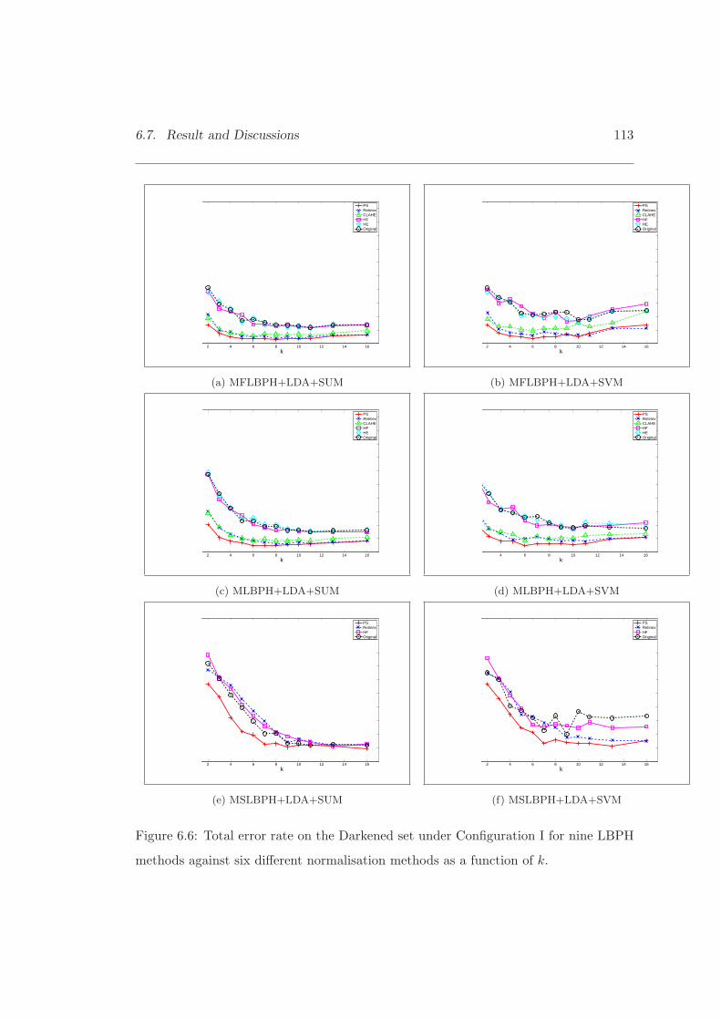
6.7. Result and Discussions 113
2 4 6 8 10 12 14 16k
PSRetinexCLAHEHFHEOriginal
(a) MFLBPH+LDA+SUM
2 4 6 8 10 12 14 16k
PSRetinexCLAHEHFHEOriginal
(b) MFLBPH+LDA+SVM
2 4 6 8 10 12 14 16k
PSRetinexCLAHEHFHEOriginal
(c) MLBPH+LDA+SUM
4 6 8 10 12 14 16k
PSRetinexCLAHEHFHEOriginal
(d) MLBPH+LDA+SVM
2 4 6 8 10 12 14 16k
PSRetinexHFOriginal
(e) MSLBPH+LDA+SUM
2 4 6 8 10 12 14 16k
PSRetinexHFOriginal
(f) MSLBPH+LDA+SVM
Figure 6.6: Total error rate on the Darkened set under Configuration I for nine LBPH
methods against six different normalisation methods as a function of k.
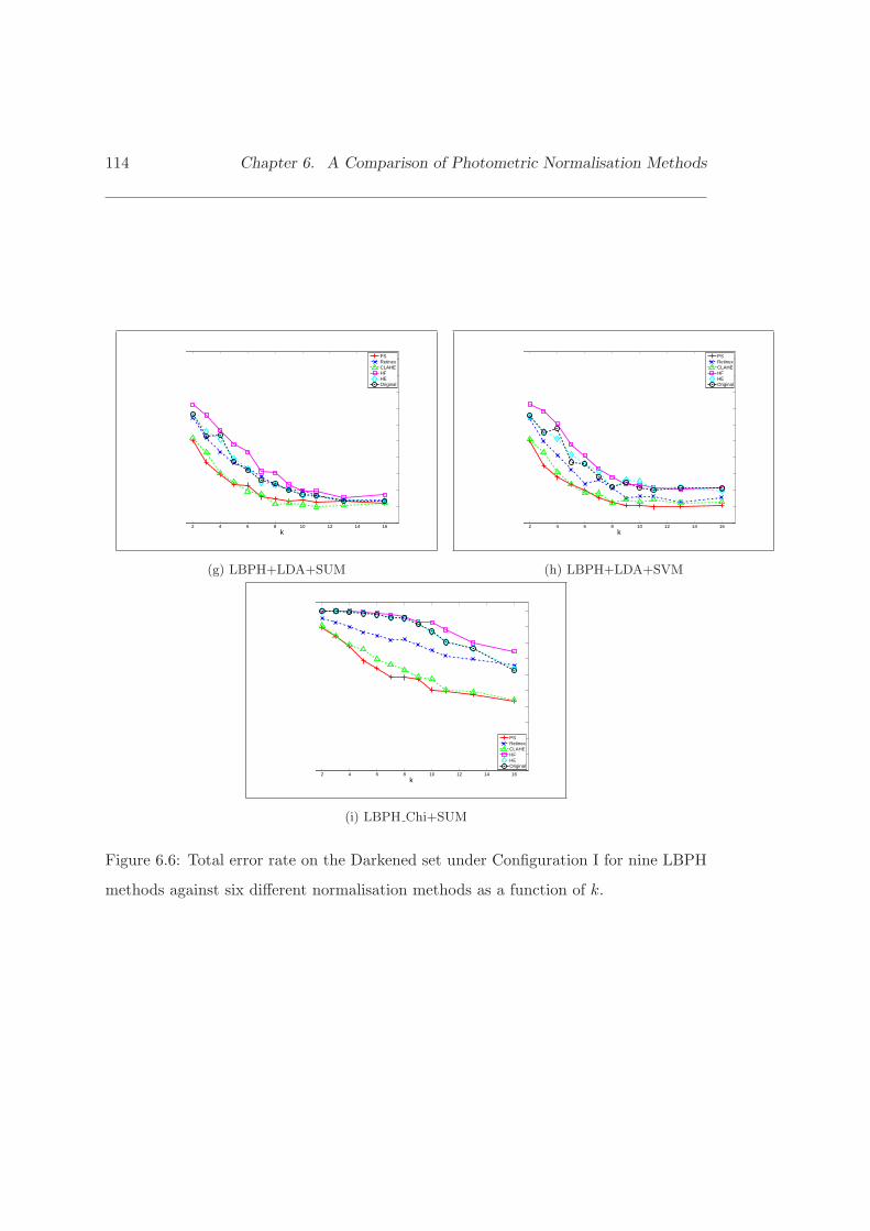
114 Chapter 6. A Comparison of Photometric Normalisation Methods
2 4 6 8 10 12 14 16k
PSRetinexCLAHEHFHEOriginal
(g) LBPH+LDA+SUM
2 4 6 8 10 12 14 16k
PSRetinexCLAHEHFHEOriginal
(h) LBPH+LDA+SVM
2 4 6 8 10 12 14 16k
PSRetinexCLAHEHFHEOriginal
(i) LBPH Chi+SUM
Figure 6.6: Total error rate on the Darkened set under Configuration I for nine LBPH
methods against six different normalisation methods as a function of k.
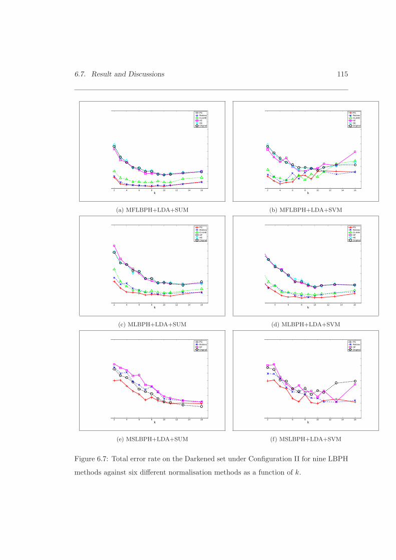
6.7. Result and Discussions 115
2 4 6 8 10 12 14 16k
PSRetinexCLAHEHFHEOriginal
(a) MFLBPH+LDA+SUM
2 4 6 8 10 12 14 16k
PSRetinexCLAHEHFHEOriginal
(b) MFLBPH+LDA+SVM
2 4 6 8 10 12 14 16k
PSRetinexCLAHEHFHEOriginal
(c) MLBPH+LDA+SUM
4 6 8 10 12 14 16k
PSRetinexCLAHEHFHEOriginal
(d) MLBPH+LDA+SVM
2 4 6 8 10 12 14 16k
PSRetinexHFOriginal
(e) MSLBPH+LDA+SUM
2 4 6 8 10 12 14 16k
PSRetinexHFOriginal
(f) MSLBPH+LDA+SVM
Figure 6.7: Total error rate on the Darkened set under Configuration II for nine LBPH
methods against six different normalisation methods as a function of k.
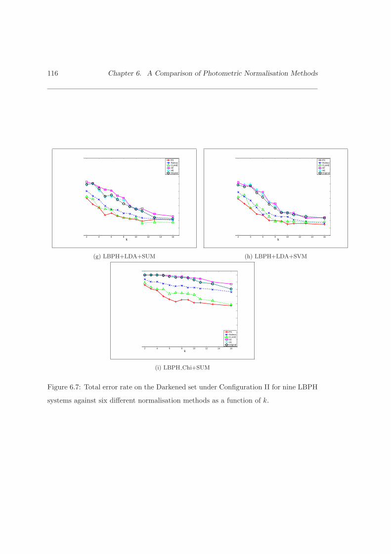
116 Chapter 6. A Comparison of Photometric Normalisation Methods
2 4 6 8 10 12 14 16k
PSRetinexCLAHEHFHEOriginal
(g) LBPH+LDA+SUM
2 4 6 8 10 12 14 16k
PSRetinexCLAHEHFHEOriginal
(h) LBPH+LDA+SVM
2 4 6 8 10 12 14 16k
PSRetinexCLAHEHFHEOriginal
(i) LBPH Chi+SUM
Figure 6.7: Total error rate on the Darkened set under Configuration II for nine LBPH
systems against six different normalisation methods as a function of k.

6.7. Result and Discussions 117
Table 6.5: Total Error Rate according to Lausanne Protocol with manual registrationConfiguration I Configuration II
k Eva Set Test Set Dark Set k Eva Set Test Set Dark Set
PS
MFLBPH+LDA+SUM 5 2.08 1.48 3.77 9 0.99 0.96 3.42
MFLBPH+LDA+SVM 11 1.07 1.12 7.70 12 0.12 0.90 12.83
MLBPH+LDA+SUM 6 2.00 1.51 4.95 10 0.99 0.99 10.34
MLBPH+LDA+SVM 16 1.05 1.54 10.81 16 0.61 1.02 13.14
MSLBPH+LDA+SUM 10 2.00 1.46 12.13 8 1.00 0.92 27.63
MSLBPH+LDA+SVM 7 2.33 1.48 13.27 11 0.49 1.06 23.28
LBPH+LDA+SUM 9 3.34 2.51 13.20 9 1.49 2.29 22.38
LBPH+LDA+SVM 16 2.34 2.67 10.82 16 1.48 2.44 14.37
LBPH Chi+SUM 16 12.39 10.25 43.17 16 7.52 7.69 56.89
Reti
nex
MFLBPH+LDA+SUM 11 1.33 0.91 5.15 11 1.00 0.68 4.67
MFLBPH+LDA+SVM 13 0.70 0.94 11.12 6 0.04 0.82 20.66
MLBPH+LDA+SUM 11 1.95 1.16 6.40 7 1.00 1.18 14.85
MLBPH+LDA+SVM 7 1.06 1.27 11.07 13 0.50 0.57 14.16
MSLBPH+LDA+SUM 7 1.66 1.69 29.42 8 1.00 1.57 42.01
MSLBPH+LDA+SVM 7 1.33 1.58 28.28 16 0.51 0.57 23.46
LBPH+LDA+SUM 10 2.66 2.37 19.94 10 15.47 13.88 82.26
LBPH+LDA+SVM 16 1.37 2.33 15.36 9 2.00 2.01 29.41
LBPH Chi+SUM 9 16.70 13.19 78.76 10 1.00 1.92 25.13
CLA
HE
MFLBPH+LDA+SUM 5 1.67 1.92 7.03 9 1.00 0.79 9.86
MFLBPH+LDA+SVM 10 1.00 1.51 15.09 8 0.50 0.86 17.69
MLBPH+LDA+SUM 5 1.99 1.79 10.11 11 1.00 0.80 14.18
MLBPH+LDA+SVM 5 1.34 1.94 13.18 7 1.00 0.76 13.40
LBPH+LDA+SUM 7 2.34 2.04 17.42 10 1.00 1.37 23.44
LBPH+LDA+SVM 7 1.98 2.32 17.76 16 1.00 1.10 18.35
LBPH Chi+SUM 11 11.90 10.18 50.40 11 8.15 7.76 66.38
HF
MFLBPH+LDA+SUM 5 1.33 1.35 21.12 10 1.00 1.03 18.68
MFLBPH+LDA+SVM 16 1.00 1.93 29.35 16 0.01 1.59 49.79
MLBPH+LDA+SUM 5 1.94 2.01 27.21 4 0.99 0.94 51.77
MLBPH+LDA+SVM 5 1.33 1.23 33.26 10 1.00 1.03 20.87
MSLBPH+LDA+SUM 10 1.91 1.17 15.95 9 1.00 0.36 35.27
MSLBPH+LDA+SVM 11 0.69 0.50 28.57 16 0.02 0.65 45.52
LBPH+LDA+SUM 7 2.32 2.32 31.36 11 0.99 0.82 36.18
LBPH+LDA+SVM 16 1.33 2.04 21.08 13 1.00 1.59 23.68
LBPH Chi+SUM 9 10.69 7.87 93.00 16 8.03 8.29 87.13
HE
MFLBPH+LDA+SUM 4 1.34 1.16 25.98 13 0.99 1.04 21.79
MFLBPH+LDA+SVM 4 1.33 1.37 31.59 16 0.41 2.01 35.37
MLBPH+LDA+SUM 5 1.74 2.05 24.83 7 1.00 1.18 33.15
MLBPH+LDA+SVM 11 1.00 1.66 21.68 11 0.99 1.39 23.06
LBPH+LDA+SUM 9 2.67 2.64 20.81 10 1.00 0.92 36.55
LBPH+LDA+SVM 16 1.24 1.89 19.57 10 1.00 1.23 30.94
LBPH Chi+SUM 7 9.98 6.86 95.75 16 6.93 7.56 79.88
Ori
gin
al
MFLBPH+LDA+SUM 4 1.34 1.16 24.97 8 1.00 0.80 22.91
MFLBPH+LDA+SVM 9 1.00 1.90 23.44 16 0.50 1.19 31.83
MLBPH+LDA+SUM 5 2.00 2.12 23.20 7 1.00 0.93 33.14
MLBPH+LDA+SVM 11 1.31 1.74 19.71 11 0.99 1.39 23.52
MSLBPH+LDA+SUM 7 1.67 1.06 20.21 9 1.00 0.44 25.78
MSLBPH+LDA+SVM 11 0.29 0.28 32.67 11 0.08 0.21 34.03
LBPH+LDA+SUM 7 2.67 2.31 26.00 7 1.00 1.26 48.55
LBPH+LDA+SVM 16 1.00 1.73 21.04 9 0.99 1.53 30.54
LBPH Chi+SUM 7 10.26 6.95 95.63 16 6.55 7.45 80.38
Oth
ers
LBP MAP [75] [56] 2.84 25.80
LBP AdaBoost [56] 7.80 71.20
LBP LDA [26] 9.12 18.22 2.86 20.88
LBP HMM [26] 2.74 19.22 1.94 19.76
ICB006-Best [58] 1.63 0.96 0.49 0.51
ICB006-Best [58] 2.35 2.02
118 Chapter 6. A Comparison of Photometric Normalisation Methods
16,028 controlled images. The uncontrolled images show serious illumination changes,
blurring and some occlusion make Experiment 4 very difficult.
Figure 6.10 presents the ROC curves of our proposed systems obtained in Experiment
1 and 4. There is not much difference in the performance of the respective systems in
Experiment 1 but MFLBPH with the preprocessing sequence (PS) method is slightly
better. In contrast to the histogram equalisation method in Experiment 4, the perfor-
mance of the preprocessing sequence method is better by a factor of two. In Experiment
1, the performance of the Retinex methods is worse than that of Histogram equalisation
and this result is different from the observations made of the in XM2VTS and Feret
databases. One of the possible reasons is that the unconstrainted training samples de-
gade the performance in Experiment 1 while improve the performance in Experiment
4. Comparing the performance with MLBPH, MFLBPH is higher by about 6% ∼10%. However, the training of MFLBPH is very time consuming, which takes almost
two weeks for computing the LDA matrices because the sample size and the feature
dimensionality are very high. Therefore, there is a trade-off between the accuracy and
computational complexity.
Table 6.6 presents comparisons with the baseline and other state-of-art methods in
Experiment 1 and 4. It is clear that our proposed method (PS MFLBPH+LDA+SUM)
is better than the baseline method in all Experiments and some of the state of art
methods in Experiment 1. However, our proposed system is worse in Experiment 4, by
around 4% ∼ 13% than the state of art methods. In contrast to the systems reported in
[91, 28], our systems only use local features which capture variations within some local
areas in the face, while their systems combine local information with global features,
capturing the whole face characteristic, to get better performance. Another possible
approach improving the performance [50, 94] is to apply the non-linear kernel method
to extract LBPH features.
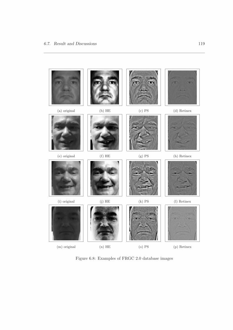
6.7. Result and Discussions 119
(a) original (b) HE (c) PS (d) Retinex
(e) original (f) HE (g) PS (h) Retinex
(i) original (j) HE (k) PS (l) Retinex
(m) original (n) HE (o) PS (p) Retinex
Figure 6.8: Examples of FRGC 2.0 database images
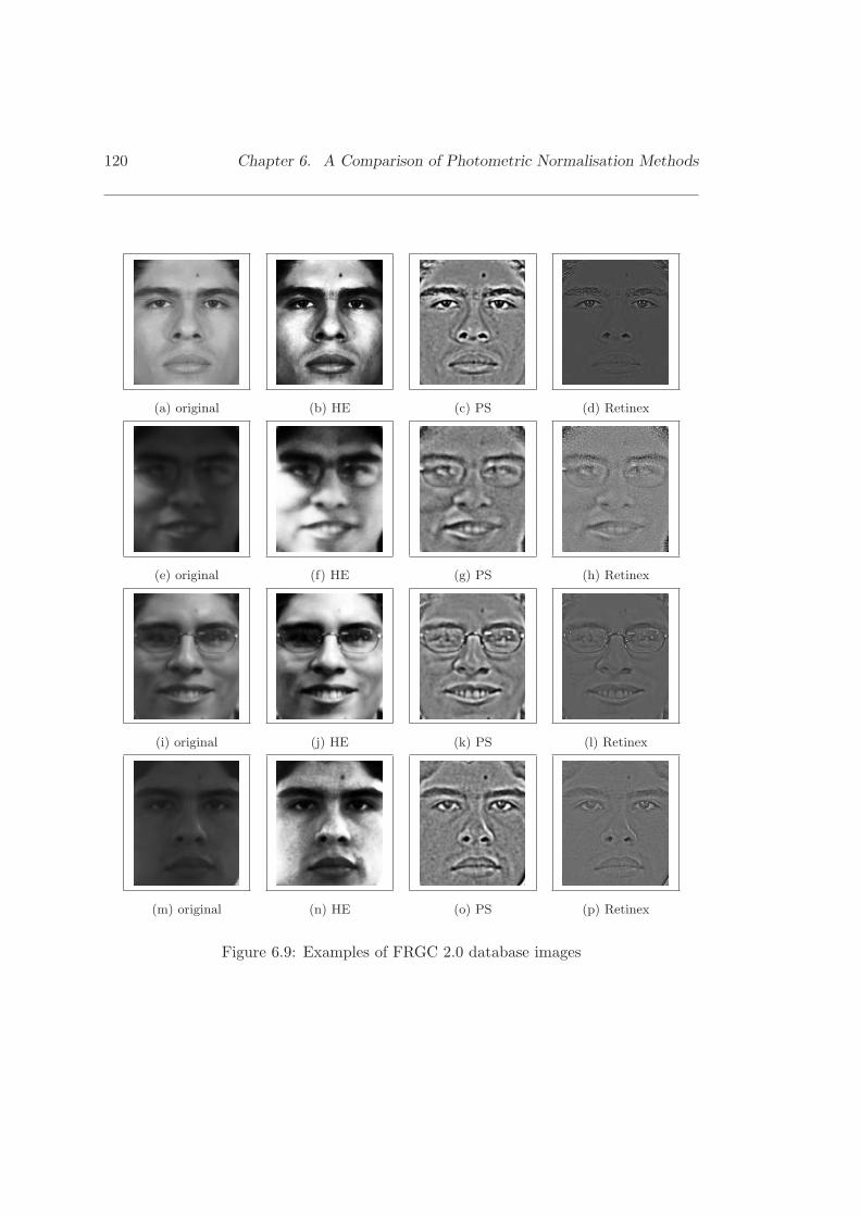
120 Chapter 6. A Comparison of Photometric Normalisation Methods
(a) original (b) HE (c) PS (d) Retinex
(e) original (f) HE (g) PS (h) Retinex
(i) original (j) HE (k) PS (l) Retinex
(m) original (n) HE (o) PS (p) Retinex
Figure 6.9: Examples of FRGC 2.0 database images
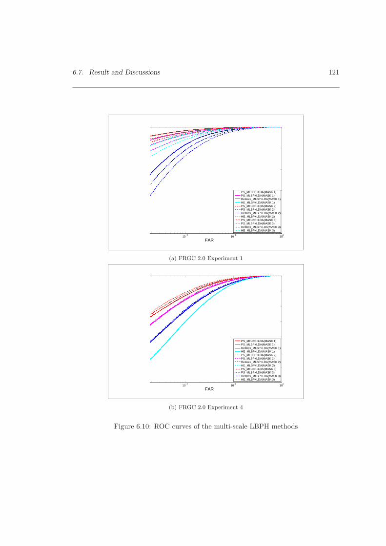
6.7. Result and Discussions 121
10−2
10−1
100
FAR
PS_MFLBP+LDA(MASK 1)PS_MLBP+LDA(MASK 1)Retinex_MLBP+LDA(MASK 1)HE_MLBP+LDA(MASK 1)PS_MFLBP+LDA(MASK 2)PS_MLBP+LDA(MASK 2)Retinex_MLBP+LDA(MASK 2)HE_MLBP+LDA(MASK 2)PS_MFLBP+LDA(MASK 3)PS_MLBP+LDA(MASK 3)Retinex_MLBP+LDA(MASK 3)HE_MLBP+LDA(MASK 3)
(a) FRGC 2.0 Experiment 1
10−2
10−1
100
FAR
PS_MFLBP+LDA(MASK 1)PS_MLBP+LDA(MASK 1)Retinex_MLBP+LDA(MASK 1)HE_MLBP+LDA(MASK 1)PS_MFLBP+LDA(MASK 2)PS_MLBP+LDA(MASK 2)Retinex_MLBP+LDA(MASK 2)HE_MLBP+LDA(MASK 2)PS_MFLBP+LDA(MASK 3)PS_MLBP+LDA(MASK 3)Retinex_MLBP+LDA(MASK 3)HE_MLBP+LDA(MASK 3)
(b) FRGC 2.0 Experiment 4
Figure 6.10: ROC curves of the multi-scale LBPH methods

122 Chapter 6. A Comparison of Photometric Normalisation Methods
Table 6.6: The verification rate in % at 0.1% FAR for different methods on FRGC 2.0
Experiment 1 and 4
Exp. 1 Exp. 4
Mask1 Mask2 Mask3 Mask1 Mask2 Mask3
PS MFLBPH+LDA+SUM 97.11 96.31 95.40 67.09 68.65 70.27
PS MLBPH+LDA+SUM 95.86 94.41 92.87 60.03 60.47 60.75
Retinex MLBPH+LDA+SUM 85.42 82.57 79.36 48.25 48.44 48.86
HE MLBPH+LDA+SUM 94.19 92.62 91.02 36.44 36.55 36.56
AMFG07’ PS LBPH+KDCV [94] 73.50
AMFG07’ PS LBPH+Gabor+KDCV [94] 83.60
ICCV07’ Gabor+Fourier+LDA+SUM [91] 98.00 86.00
PAMI06’ Gabor+KLDA [50] 92.00 76.00
CVPR06’ INGS Fourier+LDA+SUM [28] 95.01 93.29 91.51 75.70 75.06 74.33
BaseLine PCA 74.76 70.53 66.05 12.00
6.8 Summary
In order to test robustness in an unconstrained environment, LBPH face recognition
systems were evaluated with five different normalisation methods using three well-
known databases and their standard protocols. The Multi-scale Local Binary Pattern
histogram system with Preprocessing Sequence (PS) method outperformed the others
because it benefits from the inherent ability of the Multi-scale LBPH to capture the
illumination invariant information, conveyed by eye-forehead region pair, eye-nose re-
gion pair and mouth-chin region pair, reducing the effects of illumination variation,
local shadowing and highlights, while still keeping the essential visual appearance in-
formation for use in recognition. Comparing the performance with the LBPH and
6.8. Summary 123
MSLBPH systems, the Multi-scale LBPH methods in conjunction with different photo-
metric normalisation methods are robust and stable. In other words, the performance
of the Mulit-scale methods does not depend on k, but only on the effectiveness of pho-
tometric normalisation. The significance of this finding is that it helps to reduce the
time for tuning the system performance.
In face identification performed on the Feret database, the results achieved show that
the mean recognition rate of 97% at 95% confidence interval, delivered by our method
using the PS normalisation, not only outperforms other state-of-the-art contenders
which make use of Gabor Phase, the fusion of Gabor and LBP, or Local Gabor Binary
Pattern, but also further improves our proposed system presented in Section 5.6.1. In
particular, the first rank recognition rate of all probe sets except DUP2 is over 90%.
This finding indicates that the normalisation method can improve the performance of
LBPH features or even illumination invariant features.
Our proposed systems have also been tested in the verification mode on the XM2VTS
and FRGC 2.0 database with manual registration. The best overall performance of
our proposed systems in darkened set is MFLBPH+LDA+SUM with the PS method,
for which the total error rate on the test set is 3.77% for Configuration I and 3.42%
for Configuration II. Comparing with the best result published in ICB 2006 [58], our
result is around 1.7% lower. However, their approach requires the use of re-lighting
techniques to generate image samples to train the face verification system for the de-
graded lighting condition, while ours uses filtering techniques to reduce the effects of
illumination variation. In other words, our design approach is much simpler. Although
the performance of our proposed system, achieving 70% verification rate at 0.1% false
acceptance rate, is slightly worse than the best state-of-art system in the FRGC 2.0
Experiment 4, by around 4% ∼ 13%, our system is much simpler and straight forward.
In conclusion, the proposed Multi-scale Local Binary Pattern histogram system with

124 Chapter 6. A Comparison of Photometric Normalisation Methods
the Preprocessing Sequence (PS) normalisation method offers a simple and robust so-
lution to face recognition which can achieve comparable performance to the state-of-art
systems.

Chapter 7
Conclusions and Future Work
7.1 Conclusions
This thesis has presented advanced Local Binary Pattern methods for improving the
performance of 2D face recognition systems.
Chapter 1 introduced the challenges of face recognition. In Chapter 2, the main baseline
and state-of-art face recognition systems, configured from different processing modules
were discussed and summarised in Table 2.1. Motivated by a simple but powerful tex-
ture descriptor, called Local Binary Pattern, our work then focused on LBP. LBP is a
structured ordinal contrast encoding. This ordinal representation and its advantages
were described in Chapter 3. Chapter 4 introduced three well known databases and
protocols used for measuring the performance of face recognition systems. In Chapter
5, two face representations were proposed for face recognition. The first descriptor, cap-
turing the information from a multiresolution analysis of face image, called MLBPH,
was shown to provide a very robust system which is insensitive to localisation errors
because it benefits from the multiresolution information conveyed by the regional his-
125
126 Chapter 7. Conclusions and Future Work
tograms. The second proposed descriptor, namely MSLBPH, captures the mutual
relationships between neighbours at pixel level from each spectral channel and cross
spectral channel. By measuring the spatial correlation between the spectra, we expect
to achieve higher recognition rates. The regional discriminative descriptor is formed
by projecting one of these face representations into LDA space. The overall similarity
score is obtained by fusing the similarity scores of the regional descriptors.
MLBPH+LDA+SUM, LBPH+LDA+SUM, LBPH Chi+SUM and PCA MachCosine
have been evaluated on the FERET database from the point of their sensitivity to
face localisation errors. The results have shown that local region base methods clearly
outperform the PCA method. Projecting LBP histograms into an LDA space provides
better recognition rate than the original histogram space method. For the local region
based histogram methods, as the localisation error increases, the larger the region size
the better the recognition rate. Most importantly, in the presence of localisation error,
the recognition rate of MLBPH+LDA+SUM using a larger window size is more robust
than that of other methods. The main reason for the superior performance is the
proposed histogram combination approach and the multiresolution representation.
In Section 5.6.2, an unbiased fusion method (Sum-rule) and supervised classifier fusion
method (GMM and SVM) were evaluated on the XM2VTS database. The results on the
XM2VTS database have shown that the performance of MSLBPH+LDA in conjunction
with SVM is superior, for which the total error rate on the evaluation and the test set
for Configuration I is 0.29% and 0.28% respectively, and for Configuration II, 0.08%
and 0.21%.
In order to test their robustness in an unconstrained environment, the LBPH face
recognition systems were evaluated with four different normalisation methods which
are homomorphic filtering, Contrast Limited Adaptive Histogram Equalisation, the
Preprocessing Sequence approach and the Retinex approach. The multi-scale Local Bi-

7.1. Conclusions 127
nary Pattern histogram system in conjunction with the Preprocessing Sequence method
outperformed the others because it benefited from both the inherent ability of the
Multi-scale LBPH to capture illumination invariant information and the Preprocessing
Sequence approach reducing the effects of illumination variation, local shadowing and
highlights, while still keeping the essential visual appearance information for use in
recognition.
In face identification performed on the Feret database, the results achieved have shown
that the mean recognition rate of 97% at 95% confidence interval, delivered by our
method, Multi-scale Full Local Binary Pattern with LDA, (MFLBP+LDA+SUM) using
the PS normalisation, not only outperformed other state-of-the-art contenders which
make use of Gabor Phase, the fusion of Gabor and LBP, or Local Gabor Binary Pattern,
but also further improved our proposed system presented in Section 5.6.1. In particular,
the first rank recognition rate of all probe sets except DUP2 are over 90%. This finding
indicates that the normalisation method can improve the performance of LBPH features
or even illumination invariant features.
Our proposed systems have also been tested in the verification mode on the XM2VTS
and FRGC 2.0 databases with manual registration. The best overall performance of
our proposed systems on the darkened set is delivered by MFLBPH+LDA+SUM with
the PS method, for which the total error rate on the test set is 3.77% for Configuration
I and 3.42% for Configuration II. Comparing with the best result published in ICB
2006 [58], our result is around 1.7% lower. Moreover, their approach requires the use
of re-lighting techniques to generate image samples to train the face verification system
for the degraded lighting condition, while ours uses filtering techniques to reduce the
effects of illumination variation. In other words, our design approach is much simpler.
Although the performance of our proposed system, achieving 70% verification rate at
0.1% false acceptance rate, is slightly worse than the best state-of-art system in the

128 Chapter 7. Conclusions and Future Work
FRGC 2.0 Experiment 4, by around 4% ∼ 13%, our system is much simpler and straight
forward. In conclusion, the proposed Multi-scale Local Binary Pattern histogram sys-
tem with the Preprocessing Sequence (PS) normalisation method offers a simple and
robust solution to face recognition which can achieve comparable performance to the
state-of-art systems.
7.2 Future Work
This section summaries some of the many areas which have not been explored within
this thesis.
The LDA training of MFLBPH is very time consuming because of the high feature
space dimensionality. To reduce the dimensionality, the local binary patterns can be
grouped based on other criteria, such as LBP code statistics as in e.g. the Statistically
effective LBP introduced in Section 3.2.3.
In this thesis, the Multi-spectral Local Binary Pattern Histogram approach is only
applied to the problem of colour face recognition. However, it can be applied on any
multi-channel application, such as 3D face recognition. Moreover, it is also possible to
extend the Multi-scale LBPH approach to cross-resolution and cross-spectral analysis.

Bibliography
[1] Timo Ahonen, Abdenour Hadid, and Matti Pietikainen. Face recognition with
local binary patterns. In ECCV (1), pages 469–481, 2004.
[2] Timo Ahonen, Abdenour Hadid, and Matti Pietikainen. Face description with
local binary patterns: Application to face recognition. IEEE Trans. Pattern Anal.
Mach. Intell., 28(12):2037–2041, 2006.
[3] Enrique Argones-Rua, Josef Kittler, Jose Luis Alba-Castro, and Daniel Gonzalez-
Jimenez. Information fusion for local gabor features based frontal face verification.
In ICB, pages 173–181, 2006.
[4] L. Bai, L.; Shen. A fast and robust gabor feature based method for face recogni-
tion. Imaging for Crime Detection and Prevention, 2005. ICDP 2005. The IEE
International Symposium on, pages 95–98, 7-8 June 2005.
[5] M.S. Bartlett, J.R. Movellan, and T.J. Sejnowski. Face recognition by indepen-
dent component analysis. Neural Networks, IEEE Transactions on, 13(6):1450–
1464, Nov 2002.
[6] P.N. Belhumeur, J.P. Hespanha, and D.J. Kriegman. Eigenfaces vs. fisherfaces:
recognition using class specific linear projection. Transactions on Pattern Anal-
ysis and Machine Intelligence, 19(7):711–720, Jul 1997.
129

130 Bibliography
[7] P.N. Belhumeur and D.J. Kriegman. What is the set of images of an object under
all possible lighting conditions? In CVPR, page 270, Los Alamitos, CA, USA,
1996. IEEE Computer Society.
[8] J.R. Beveridge, K. She, B.A. Draper, and G.H. Givens. A nonparametric statisti-
cal comparison of principal component and linear discriminant subspaces for face
recognition. In Computer Vision and Pattern Recognition, 2001. CVPR 2001.
Proceedings of the 2001 IEEE Computer Society Conference on, volume 1, pages
I–535–I–542 vol.1, 2001.
[9] William L. Briggs, Van Emden Henson, and Steve F. McCormick. A multigrid
tutorial. Society for Industrial and Applied Mathematics, Philadelphia, PA, USA,
1987.
[10] Chi-Ho Chan, Josef Kittler, and Kieron Messer. Multi-scale local binary pattern
histograms for face recognition. In Seong-Whan Lee and Stan Z. Li, editors, ICB,
volume 4642 of Lecture Notes in Computer Science, pages 809–818. Springer,
2007.
[11] Chi-Ho Chan, Josef Kittler, and Kieron Messer. Multispectral local binary pat-
tern histogram for component-based color face verification. In Biometrics: The-
ory, Applications, and Systems, 2007. BTAS 2007. First IEEE International
Conference on, pages 1–7, 27-29 Sept. 2007.
[12] Nitesh V. Chawla and Kevin W. Bowyer. Random subspaces and subsampling
for 2-d face recognition. In CVPR (2), pages 582–589, 2005.
[13] Li-Fen Chen, Hong-Yuan Mark Liao, Ming-Tat Ko, Ja-Chen Lin, and Gwo-Jong
Yu. A new lda-based face recognition system which can solve the small sample
size problem. Pattern Recognition, 33(10):1713–1726, 2000.

Bibliography 131
[14] X. Chen, S. Shan, B. Cao, X. Chen, and W. Gao. Multiple fisher classifiers
combination for face recognition based on grouping adaboosted gabor features.
In BMVC05, pages 569–578, 2005.
[15] H. Chengjun Liu; Wechsler. Gabor feature based classification using the enhanced
fisher linear discriminant model for face recognition. Image Processing, IEEE
Transactions on, 11(4):467–476, Apr 2002.
[16] J.G. Daugman. High confidence visual recognition of persons by a test of statisti-
cal independence. Pattern Analysis and Machine Intelligence, IEEE Transactions
on, 15(11):1148–1161, Nov 1993.
[17] Hazim Kemal Ekenel and Rainer Stiefelhagen. Analysis of local appearance-
based face recognition: Effects of feature selection and feature normalization. In
CVPRW ’06: Proceedings of the 2006 Conference on Computer Vision and Pat-
tern Recognition Workshop, page 34, Washington, DC, USA, 2006. IEEE Com-
puter Society.
[18] H.K. Ekenel, J. Stallkamp, H. Gao, M. Fischer, and R. Stiefelhagen. Face recog-
nition for smart interactions. In Multimedia and Expo, 2007 IEEE International
Conference on, pages 1007–1010, 2-5 July 2007.
[19] Mario A. T. Figueiredo and Anil K. Jain. Unsupervised learning of finite mixture
models. IEEE Trans. Pattern Anal. Mach. Intell., 24(3):381–396, 2002.
[20] Keinosuke Fukunaga. Introduction to statistical pattern recognition (2nd ed.).
Academic Press Professional, Inc., San Diego, CA, USA, 1990.
[21] Athinodoros S. Georghiades, David J. Kriegman, and Peter N. Belhumeur. Illu-
mination cones for recognition under variable lighting: Faces. In CVPR, pages
52–59, 1998.
132 Bibliography
[22] J.L. Gonzalez-Jimenez, D.; Alba-Castro. Shape contexts and gabor features for
face description and authentication. Image Processing, 2005. ICIP 2005. IEEE
International Conference on, 2:II–962–5, 11-14 Sept. 2005.
[23] Ralph Gross and Vladimir Brajovic. An image preprocessing algorithm for illumi-
nation invariant face recognition. In 4th International Conference on Audio- and
Video-Based Biometric Person Authentication (AVBPA). Springer, June 2003.
[24] Abdenour Hadid, Matti Pietikainen, and Stan Z. Li. Learning personal specific
facial dynamics for face recognition from videos. In AMFG, pages 1–15, 2007.
[25] B. Heisele, P. Ho, and T. Poggio. Face recognition with support vector machines:
global versus component-based approach. In Computer Vision, 2001. ICCV 2001.
Proceedings. Eighth IEEE International Conference on, volume 2, pages 688–694
vol.2, 2001.
[26] Guillaume Heusch, Yann Rodriguez, and Sebastien Marcel. Local binary patterns
as an image preprocessing for face authentication. In FGR ’06: Proceedings of the
7th International Conference on Automatic Face and Gesture Recognition, pages
9–14, Washington, DC, USA, 2006. IEEE Computer Society.
[27] Xiangsheng Huang, Stan Z. Li, and Yangsheng Wang. Jensen-shannon boosting
learning for object recognition. In CVPR (2), pages 144–149, 2005.
[28] Wonjun Hwang, Gyutae Park, Jongha Lee, and Seok-Cheol Kee. Multiple face
model of hybrid fourier feature for large face image set. In CVPR ’06: Proceedings
of the 2006 IEEE Computer Society Conference on Computer Vision and Pattern
Recognition, pages 1574–1581, Washington, DC, USA, 2006. IEEE Computer
Society.

Bibliography 133
[29] Jonathon Phillips Hyeonjoon Moon. Analysis of pca-based face recognition algo-
rithms. Empirical Evaluation Techniques in Computer Vision, 1998.
[30] P Jonathon Phillips Hyeonjoon Moon. Computational and performance aspects
of pca-based face-recognition algorithms. Perception, 30(3):303–321, 2001.
[31] Anil K. Jain and Stan Z. Li. Handbook of Face Recognition. Springer-Verlag New
York, Inc., Secaucus, NJ, USA, 2004.
[32] D.J. Jobson, Z. Rahman, and G.A. Woodell. A multiscale retinex for bridging the
gap between color images and the human observation of scenes. Image Processing,
IEEE Transactions on, 6(7):965–976, Jul 1997.
[33] III Jones, C. and A.L. Abbott. Color face recognition by hypercomplex gabor
analysis. In Automatic Face and Gesture Recognition, 2006. FGR 2006. 7th In-
ternational Conference on, pages 6 pp.–, 10-12 April 2006.
[34] Kenneth Jonsson, Josef Kittler, Yongping Li, and Jiri Matas. Learning support
vectors for face verification and recognition. In FG, pages 208–213, 2000.
[35] A.N. Juwei Lu; Plataniotis, K.N.; Venetsanopoulos. Face recognition using lda-
based algorithms. Neural Networks, IEEE Transactions on, 14(1):195–200, Jan
2003.
[36] Tae-Kyun Kim, Hyunwoo Kim, Wonjun Hwang, and Josef Kittler. Component-
based lda face description for image retrieval and mpeg-7 standardisation. Image
Vision Comput., 23(7):631–642, 2005.
[37] Tae-Kyun Kim and Josef Kittler. Locally linear discriminant analysis for multi-
modally distributed classes for face recognition with a single model image. IEEE
Transactions on Pattern Analysis and Machine Intelligence, 27(3):318–327, 2005.

134 Bibliography
[38] J Kittler, Y P Li, and J Matas. On matching scores for lda-based face. In
BMVC00, 2000.
[39] M. Lades, J.C. Vorbruggen, J. Buhmann, J. Lange, C. von der Malsburg, R.P.
Wurtz, and W. Konen. Distortion invariant object recognition in the dynamic
link architecture. Computers, IEEE Transactions on, 42(3):300–311, Mar 1993.
[40] O. Lahdenoja, J. Maunu, M. Laiho, and A. Paasio. A massively parallel algorithm
for local binary pattern based face recognition. In Circuits and Systems, 2006.
ISCAS 2006. Proceedings. 2006 IEEE International Symposium on, pages 4 pp.–,
21-24 May 2006.
[41] Kin-Man Lam and Hong Yan. An analytic-to-holistic approach for face recogni-
tion based on a single frontal view. Pattern Analysis and Machine Intelligence,
IEEE Transactions on, 20(7):673–686, Jul 1998.
[42] Kuang-Chih Lee, Jeffrey Ho, and David J. Kriegman. Nine points of light: Ac-
quiring subspaces for face recognition under variable lighting. In CVPR (1), pages
519–526, 2001.
[43] Stan Z. Li, Rufeng Chu, ShengCai Liao, and Lun Zhang. Illumination invariant
face recognition using near-infrared images. IEEE Trans. Pattern Anal. Mach.
Intell., 29(4):627–639, 2007.
[44] Stan Z. Li, RuFeng Chu, ShengCai Liao, and Lun Zhang. Illumination invari-
ant face recognition using near-infrared images. Pattern Analysis and Machine
Intelligence, IEEE Transactions on, 29(4):627–639, April 2007.
[45] Stan Z. Li, ChunShui Zhao, Meng Ao, , and Zhen Lei. Learning to fuse 3d+2d
based face recognition at both feature and decision levels. In Analysis and Mod-
elling of Faces and Gestures, pages 44–54. Springer Berlin / Heidelberg, 2005.

Bibliography 135
[46] Stan Z. Li, ChunShui Zhao, Meng Ao, and Zhen Lei. Learning to fuse 3d+2d
based face recognition at both feature and decision levels. In AMFG, pages 44–54,
2005.
[47] Yongping Li. Linear Discriminant Analysis and its application to Face Identifi-
cation. PhD thesis, University of Surrey, 2000.
[48] ShengCai Liao, Zhen Lei, XiangXin Zhu, Zhenan Sun, Stan Z. Li, and Tieniu
Tan. Face recognition using ordinal features. In ICB, pages 40–46, 2006.
[49] ShengCai Liao, XiangXin Zhu, Zhen Lei, Lun Zhang, and Stan Z. Li. Learning
multi-scale block local binary patterns for face recognition. In ICB, pages 828–
837, 2007.
[50] Chengjun Liu. Capitalize on dimensionality increasing techniques for improving
face recognition grand challenge performance. IEEE Trans. Pattern Anal. Mach.
Intell., 28(5):725–737, 2006.
[51] Chengjun Liu and H. Wechsler. Gabor feature based classification using the
enhanced fisher linear discriminant model for face recognition. Image Processing,
IEEE Transactions on, 11(4):467–476, Apr 2002.
[52] Chengjun Liu and Harry Wechsler. Gabor feature based classification using the
enhanced fisher linear discriminant model for face recognition. IEEE Transactions
on Image Processing, 11(4):467–476, 2002.
[53] Topi Maenpaa, Timo Ojala, Matti Pietikainen, and Soriano Maricor. Robust
texture classification by subsets of local binary patterns. In Pattern Recognition,
International Conference on, volume 3, page 3947, Los Alamitos, CA, USA, 2000.
IEEE Computer Society.

136 Bibliography
[54] Topi Maenpaa and Matti Pietikainen. Multi-scale binary patterns for texture
analysis. In SCIA, pages 885–892, 2003.
[55] Topi Maenpaa, Matti Pietikainen, and Jaakko Viertola. Separating color and
pattern information for color texture discrimination. In Pattern Recognition,
International Conference on, volume 1, pages 668–671, 2002.
[56] Sebastien Marcel, Yann Rodriguez, and Guillaume Heusch. On the recent use
of local binary patterns for face authentication. International Journal on Image
and Video Processing Special Issue on Facial Image Processing, 2007. IDIAP-RR
06-34.
[57] K. Messer, J. Matas, J. Kittler, J. Luttin, and G. Maitre. XM2VTSDB: The
extended M2VTS database. In Audio- and Video-based Biometric Person Au-
thentication, AVBPA’99, pages 72–77, 1999. Washington, D.C., March 1999. 16
IDIAP–RR 99-02.
[58] Kieron Messer, Josef Kittler, James Short, Guillaume Heusch, Fabien Cardinaux,
Sebastien Marcel, Yann Rodriguez, Shiguang Shan, Y. Su, Wen Gao, and Xilin
Chen. Performance characterisation of face recognition algorithms and their sen-
sitivity to severe illumination changes. In ICB, pages 1–11, 2006.
[59] B. Moghaddam, C. Nastar, and A. Pentland. A bayesian similarity measure for
direct image matching. icpr, 02:350, 1996.
[60] A.V. Nefian and III Hayes, M.H. Hidden markov models for face recognition.
Acoustics, Speech and Signal Processing, 1998. Proceedings of the 1998 IEEE
International Conference on, 5:2721–2724 vol.5, 12-15 May 1998.
[61] Timo Ojala, Matti Pietikainen, and Topi Maenpaa. Multiresolution gray-scale
Bibliography 137
and rotation invariant texture classification with local binary patterns. IEEE
Transactions on Pattern Analysis and Machine Intelligence, 24(7):971–987, 2002.
[62] Pekka Paalanen, Joni-Kristian Kamarainen, Jarmo Ilonen, and Heikki
Kalviainen. Gmmbayes - gaussian mixture model methods, April 2005.
http://www.it.lut.fi/project/gmmbayes/.
[63] A. Pentland, B. Moghaddam, and T. Starner. View-based and modular
eigenspaces for face recognition. In Computer Vision and Pattern Recognition,
1994. Proceedings CVPR ’94., 1994 IEEE Computer Society Conference on, pages
84–91, 21-23 Jun 1994.
[64] Vytautas Perlibakas. Distance measures for pca-based face recognition. Pattern
Recogn. Lett., 25(6):711–724, 2004.
[65] P. Jonathon Phillips. Support vector machines applied to face recognition. In
NIPS, pages 803–809, 1998.
[66] P. Jonathon Phillips. Support vector machines applied to face recognition. In
Proceedings of the 1998 conference on Advances in neural information processing
systems II, pages 803–809, Cambridge, MA, USA, 1999. MIT Press.
[67] P. Jonathon Phillips, Patrick J. Flynn, W. Todd Scruggs, Kevin W. Bowyer,
Jin Chang, Kevin Hoffman, Joe Marques, Jaesik Min, and William J. Worek.
Overview of the face recognition grand challenge. In CVPR (1), pages 947–954,
2005.
[68] P. Jonathon Phillips, Hyeonjoon Moon, Patrick Rauss, and Syed A. Rizvi. The
feret evaluation methodology for face-recognition algorithms. In cvpr, page 137,
Los Alamitos, CA, USA, 1997. IEEE Computer Society.

138 Bibliography
[69] P. Jonathon Phillips, Hyeonjoon Moon, Syed A. Rizvi, and Patrick J. Rauss.
The feret evaluation methodology for face-recognition algorithms. IEEE Trans.
Pattern Anal. Mach. Intell., 22(10):1090–1104, 2000.
[70] Matti Pietikainen, Timo Ojala, Jarkko Nisula, and Jouni Heikkinen. Experi-
ments with two industrial problems using texture classification based on feature
distributions. Intelligent Robots and Computer Vision XIII: 3D Vision, Product
Inspection, and Active Vision, 2354(1):197–204, 1994.
[71] Matti Pietikainen, Timo Ojala, and Z. Xu. Rotation-invariant texture classifica-
tion using feature distributions. Pattern Recognition, 33:43–52, 2000.
[72] Stephen M. Pizer, E. Philip Amburn, John D. Austin, Robert Cromartie, Ari
Geselowitz, Trey Greer, Bart Ter Haar Romeny, and John B. Zimmerman. Adap-
tive histogram equalization and its variations. Comput. Vision Graph. Image
Process., 39(3):355–368, 1987.
[73] Laiyun Qing, Shiguang Shan, Xilin Chen, and Wen Gao. Face recognition under
varying lighting based on the probabilistic model of gabor phase. In Pattern
Recognition, 2006. ICPR 2006. 18th International Conference on, volume 3, pages
1139–1142, 2006.
[74] Y. Raja and S. Gong. Sparse multiscale local binary patterns. In British Machine
Vision Conference, volume 2, pages 799–808, September 2006.
[75] Yann Rodriguez and Sebastien Marcel. Face authentication using adapted local
binary pattern histograms. In ECCV (4), pages 321–332, 2006.
[76] Marcio Teixeira Ross Beveridge, David Bolme and Bruce Draper. The CSU Face
Identification Evaluation System User’s Guide: Version 5.0., 2003.

Bibliography 139
[77] Javid Sadr, Sayan Mukherjee, K. Thoresz, and Pawan Sinha. The fidelity of local
ordinal encoding. In NIPS, pages 1279–1286, 2001.
[78] Robert E. Schapire. A brief introduction to boosting. In IJCAI ’99: Proceedings
of the Sixteenth International Joint Conference on Artificial Intelligence, pages
1401–1406, San Francisco, CA, USA, 1999. Morgan Kaufmann Publishers Inc.
[79] Anton Schwaighofer. Svm toolbox for matlab, January 2002.
http://ida.first.fraunhofer.de/ anton/software.html.
[80] Shiguang Shan, Yizheng Chang, Wen Gao, Bo Cao, and Peng Yang. Curse of
mis-alignment in face recognition: Problem and a novel mis-alignment learning
solution. In FGR, pages 314–320, 2004.
[81] Shiguang Shan, Peng Yang, Xilin Chen, and Wen Gao. Adaboost gabor fisher
classifier for face recognition. In AMFG, pages 279–292, 2005.
[82] Shiguang Shan, Wenchao Zhang, Yu Su, Xilin Chen, and Wen Gao. Ensemble
of piecewise fda based on spatial histograms of local (gabor) binary patterns for
face recognition. In ICPR (4), pages 606–609, 2006.
[83] LinLin Shen and Li Bai. Gabor wavelets and kernel direct discriminant analysis
for face recognition. In ICPR (1), pages 284–287, 2004.
[84] LinLin Shen and Li Bai. Mutualboost learning for selecting gabor features for
face recognition. Pattern Recognition Letters, 27(15):1758–1767, 2006.
[85] LinLin Shen, Li Bai, Daniel Bardsley, and Yangsheng Wang. Gabor feature
selection for face recognition using improved adaboost learning. In IWBRS, pages
39–49, 2005.

140 Bibliography
[86] James Short, Josef Kittler, and Kieron Messer. Photometric normalisation for
component-based face verification. In FG, pages 114–119, 2006.
[87] Pawan Sinha. Qualitative representations for recognition. In BMCV ’02: Proceed-
ings of the Second International Workshop on Biologically Motivated Computer
Vision, pages 249–262, London, UK, 2002. Springer-Verlag.
[88] Yu Su, Shiguang Shan, Bo Cao, Xilin Chen, and Wen Gao. Hierarchical ensemble
of gabor fisher classifier for face recognition. In FG, pages 91–96, 2006.
[89] Yu Su, Shiguang Shan, Xilin Chen, and Wen Gao. Multiple fisher classifiers
combination for face recognition based on grouping adaboosted gabor features.
In BMVC, 2006.
[90] Yu Su, Shiguang Shan, Xilin Chen, and Wen Gao. Patch-based gabor fisher
classifier for face recognition. In ICPR (2), pages 528–531, 2006.
[91] Yu Su, Shiguang Shan, Xilin Chen, and Wen Gao. Hierarchical ensemble of global
and local classifiers for face recognition. In ICCV, pages 1–8, Oct. 2007.
[92] Zhenan Sun, Tieniu Tan, Yunhong Wang, and Stan Z. Li. Ordinal palmprint
represention for personal identification. In CVPR (1), pages 279–284, 2005.
[93] Xiaoyang Tan and Bill Triggs. Enhanced local texture feature sets for face recog-
nition under difficult lighting conditions. In Shaohua Kevin Zhou, Wenyi Zhao,
Xiaoou Tang, and Shaogang Gong, editors, AMFG, volume 4778 of Lecture Notes
in Computer Science, pages 168–182. Springer, 2007.
[94] Xiaoyang Tan and Bill Triggs. Fusing gabor and lbp feature sets for kernel-based
face recognition. In AMFG, pages 235–249, 2007.

Bibliography 141
[95] Marcio Luis Teixeira. The bayesian intrapersonal/extrapersonal classifier. Mas-
ter’s thesis, CSU Computer Science Department, July 2003.
[96] Keith John Thoresz. Qualitative representations for recognition. Master’s thesis,
MIT, July 2002.
[97] Ulrich Trottenberg, Cornelis Oosterlee, and Anton Schuller. MULTIGRID. Aca-
demic Press, San Diego, California 92101-4495, USA, 2001.
[98] A.P. Turk, M.A.; Pentland. Face recognition using eigenfaces. In Computer
Vision and Pattern Recognition, 1991. Proceedings CVPR ’91., IEEE Computer
Society Conference on, pages 586–591, 3-6 Jun 1991.
[99] Paul Viola and Michael J. Jones. Robust real-time face detection. Int. J. Comput.
Vision, 57(2):137–154, 2004.
[100] Haitao Wang, Stan Z. Li, and Yangsheng Wang. Face recognition under varying
lighting conditions using self quotient image. In FGR, pages 819–824, 2004.
[101] Xiaogang Wang and Xiaoou Tang. Bayesian face recognition using gabor features.
In WBMA ’03: Proceedings of the 2003 ACM SIGMM workshop on Biometrics
methods and applications, pages 70–73, New York, NY, USA, 2003. ACM.
[102] P.C. Wei-Shi Zheng; Jian-Huang Lai; Yuen. Ga-fisher: a new lda-based face
recognition algorithm with selection of principal components. Systems, Man, and
Cybernetics, Part B, IEEE Transactions on, 35(5):1065–1078, Oct. 2005.
[103] Laurenz Wiskott, Jean-Marc Fellous, Norbert Kruger, and Christoph von der
Malsburg. Face recognition by elastic bunch graph matching. IEEE Trans. on
Pattern Analysis and Machine Intelligence, 19(7):775–779, 1997.
142 Bibliography
[104] K.; Wang Shitong Wu Xiao-Jun; Kittler, J.; Yang Jing-Yu; Messer. A new di-
rect lda (d-lda) algorithm for feature extraction in face recognition. In ICPR
2004. Proceedings of the 17th International Conference on Pattern Recognition,
volume 4, pages 545–548 Vol.4, 23-26 Aug. 2004.
[105] Rong Xiao, Wujun Li, Yuandong Tian, and Xiaoou Tang. Joint boosting fea-
ture selection for robust face recognition. In CVPR ’06: Proceedings of the 2006
IEEE Computer Society Conference on Computer Vision and Pattern Recogni-
tion, pages 1415–1422, Washington, DC, USA, 2006. IEEE Computer Society.
[106] P.; Hong-Jiang Zhang Xiaofei He; Shuicheng Yan; Yuxiao Hu; Niyogi. Face
recognition using laplacianfaces. Transactions on Pattern Analysis and Machine
Intelligence, 27(3):328–340, March 2005.
[107] Chunyan Xie and B. V. K. Vijaya Kumar. Quaternion correlation filters for color
face recognition. In Security, Steganography, and Watermarking of Multimedia
Contents, pages 486–494, 2005.
[108] Xun Xu and Thomas S. Huang. Face recognition with mrc-boosting. In ICCV,
pages 1770–1777, 2005.
[109] Wendy S. Yambor. Analysis of pca-based and fisher discriminant-based image
recognition algorithms. Master’s thesis, CSU Computer Science Department, July
2003.
[110] Jian Yang and Jing-Yu Yang. Why can lda be performed in pca transformed
space? Pattern Recognition, 36(2):563–566, 2003.
[111] Ming-Hsuan Yang, David J. Kriegman, and Narendra Ahuja. Detecting faces in
images: A survey. IEEE Trans. Pattern Anal. Mach. Intell., 24(1):34–58, 2002.

Bibliography 143
[112] Peng Yang, Shiguang Shan, Wen Gao, Stan Z. Li, and Dong Zhang. Face recog-
nition using ada-boosted gabor features. In FGR, pages 356–361, 2004.
[113] Jieping Ye and Qi Li. A two-stage linear discriminant analysis via qr-
decomposition. IEEE Trans. Pattern Anal. Mach. Intell., 27(6):929–941, 2005.
[114] Hua Yu and Jie Yang. A direct lda algorithm for high-dimensional data - with
application to face recognition. Pattern Recognition, 34(10):2067–2070, 2001.
[115] Ramin Zabih and John Woodfill. Non-parametric local transforms for computing
visual correspondence. In ECCV (2), pages 151–158, 1994.
[116] B. Zhang, S. Shan, X. Chen, and W. Gao. Histogram of gabor phase patterns
(hgpp): A novel object representation approach for face recognition. Image Pro-
cessing, IEEE Transactions on, 16(1):57–68, Jan. 2007.
[117] Baochang Zhang. Gabor-kernel fisher analysis for face recognition. In PCM (2),
pages 802–809, 2004.
[118] Baochang Zhang, Wen Gao, Shiguang Shan, and Peng Yang. Discriminant gabor-
faces and support vector machines classifier for face recognition. In ACCV, pages
37–41. Springer, Jan 2004.
[119] Baochang Zhang, Peng Yang, Shiguang Shan, and Wen Gao. Discriminant gabor-
faces and support vector machines classifier for face recognition. In ACCV, pages
37–41, 2004.
[120] Guangcheng Zhang, Xiangsheng Huang, Stan Z. Li, Yangsheng Wang, and Xihong
Wu. Boosting local binary pattern (lbp)-based face recognition. In SINOBIO-
METRICS, pages 179–186, 2004.
144 Bibliography
[121] Lei Zhang, S.Z. Li, Zhi Yi Qu, and Xiangsheng Huang. Boosting local feature
based classifiers for face recognition. In Computer Vision and Pattern Recognition
Workshop, 2004 Conference on, pages 87–87, 27-02 June 2004.
[122] Wenchao Zhang, Shiguang Shan, Xilin Chen, and Wen Gao. Local gabor binary
patterns based on mutual information for face recognition. Int. J. Image Graphics,
7(4):777–793, 2007.
[123] Wenchao Zhang, Shiguang Shan, Laiyun Qing, Xilin Chen, and Wen Gao. Are ga-
bor phases really useless for face recognition? Pattern Analysis and Applications,
May 2008.
[124] Guoying Zhao and Matti Pietikainen. Dynamic texture recognition using local
binary patterns with an application to facial expressions. IEEE Transactions on
Pattern Analysis and Machine Intelligence, 29(6):915–928, 2007.
[125] Jiali Zhao, Haitao Wang, Haibing Ren, and Seok-Cheol Kee. Lbp discriminant
analysis for face verification. In Computer Vision and Pattern Recognition, 2005
IEEE Computer Society Conference on, volume 3, pages 167–167, 20-26 June
2005.
[126] W. Zhao, R. Chellappa, P. J. Phillips, and A. Rosenfeld. Face recognition: A
literature survey. ACM Comput. Surv., 35(4):399–458, 2003.
[127] Xuan Zou, Josef Kittler, and Kieron Messer. Motion compensation for face recog-
nition based on active differential imaging. In ICB, pages 39–48, 2007.
[128] Karel Zuiderveld. Contrast limited adaptive histogram equalization. Graphics
gems IV, pages 474–485, 1994.


![Scene classification using local and global features with ...In [8], the pyramid histogram of multi-scale block local binary pattern (PH-MBLBP) descriptor was employed, which can encode](https://static.fdocuments.us/doc/165x107/601f7320b51bcd0ca105fd15/scene-classification-using-local-and-global-features-with-in-8-the-pyramid.jpg)


![[1] Efficient manipulation of binary data using pattern matching](https://static.fdocuments.us/doc/165x107/62063fcb8c2f7b173005d9f8/1-efficient-manipulation-of-binary-data-using-pattern-matching.jpg)