Multi-objective optimization of electric-discharge ...

Journal of Mechanical Science and Technology 26 (6) (2012) 1875~1883 www.springerlink.com/content/1738-494x

DOI 10.1007/s12206-012-0411-x

Multi-objective optimization of electric-discharge machining process using

controlled elitist NSGA-II† Pushpendra S. Bharti1,*, S. Maheshwari2 and C. Sharma3

1U.S.E.T., Guru Gobind Singh Indraprastha University, Delhi-110006, India 2MPAE Division, Netaji Subhas Institute of Technology, Delhi-110078, India

3Department of MAE, Indira Gandhi Institute of Technology, Delhi-110006, India

(Manuscript Received November 30, 2010; Revised April 16, 2011; Accepted July 17, 2011)

----------------------------------------------------------------------------------------------------------------------------------------------------------------------------------------------------------------------------------------------------------------------------------------------

Abstract Parametric optimization of electric discharge machining (EDM) process is a multi-objective optimization task. In general, no single

combination of input parameters can provide the best cutting speed and the best surface finish simultaneously. Genetic algorithm has been proven as one of the most popular multi-objective optimization techniques for the parametric optimization of EDM process. In this work, controlled elitist non-dominated sorting genetic algorithm has been used to optimize the process. Experiments have been carried out on die-sinking EDM by taking Inconel 718 as work piece and copper as tool electrode. Artificial neural network (ANN) with back propagation algorithm has been used to model EDM process. ANN has been trained with the experimental data set. Controlled elitist non-dominated sorting genetic algorithm has been employed in the trained network and a set of pareto-optimal solutions is obtained.

Keywords: Artificial neural networks; Electric discharge machining; Genetic algorithm; Material removal rate; Optimization; Pareto-optimal solutions;

Surface roughness. ---------------------------------------------------------------------------------------------------------------------------------------------------------------------------------------------------------------------------------------------------------------------------------------------- 1. Introduction

Inconel 718 is one of the most difficult-to-cut nickel based alloys. Formation of complex shapes (of this material) along with reasonable speed and surface finish is very difficult by traditional machining. Electric discharge machining (EDM) is one of the most suitable non-conventional material removal processes to shape this alloy. EDM is a thermo-electric proc-ess in which material is removed from work piece by erosion effect of series of electric discharges (sparks) between tool and work piece immersed in a dielectric liquid. The EDM process has a very strong stochastic nature due to the complicated discharge mechanisms making it difficult to optimize the process [1]. The process performance can be improved by selecting the optimal combination of process parameters. Op-timization of process parameters of EDM is a multi-objective optimization task as, in practice, the performance measures (Material Removal Rate and Surface Roughness) are conflict-ing in nature. Though much work has been reported in litera-ture to improve the process performance, proper selection of process parameters still remains a challenge. There are several multi-objective optimization techniques for the same like goal

programming, simulated annealing (SA), grey relation, and genetic algorithms (GA).

SA is an optimization process whose operation is strongly reminiscent of the physical annealing of crystalline com-pounds such as metals and metallic alloys [2]. Tarng et al. [3] and Yang et al. [4] employed SA technique for optimizing the parameters of EDM. Grey relation analysis has been em-ployed successfully as a multi-objective optimization tech-nique in EDM by many authors [5-7].

Literature review shows that to employ SA, two objectives are transformed into a single objective by simple weighted method in which weight values are user defined in the range of 0 and 1. A single combination of input parameters has gen-erally been reported in literature by employing SA. In grey relation method also, the authors (in literature) have generally reported a single combination of input parameters as optimal combination corresponding to the grey relation grade of higher rank. Since, the performance measures are conflicting in nature in case of EDM, a single combination does not pro-vide satisfactory solutions for the best performance measures simultaneously. In some of the classical techniques, multi-objective optimization problem is directly converted to a sin-gle-optimization problem which deviates from the exact solu-tions. Some of the techniques terminate at local optima and global optimum solutions are not reached. As a result, the true optimal solutions are not obtained.

*Corresponding author. Tel.: +91 9810478041 E-mail address: [email protected]

† Recommended by Associate Editor Yong-Tae Kim © KSME & Springer 2012

1876 P. S. Bharti et al. / Journal of Mechanical Science and Technology 26 (6) (2012) 1875~1883

GA is very different from most of the traditional optimiza-tion methods. GA finds applicability in the field of EDM. It works with a random population of solution points and a set of pareto-optimal solutions is obtained for the best performance measures.

Su et al. [8] optimized the process parameters of EDM by employing GA. A neural network was trained to establish the relationships between process parameters and performance measures and then GA was adapted to the trained network to determine the optimal process parameters. Mandal et al. [9] used ANN for modeling EDM process and then employed non-dominating sorting genetic algorithm-II (NSGA-II) to find pareto-optimal solutions. Kuriakose and Shunmugan [10] employed NSGA to optimize the EDM process. There are many references where GA has been applied as a multi-objective optimization technique in the field of EDM [11-14].

There are several variants of GA like multi-objective ge-netic algorithm (MOGA), vector evaluated genetic algorithm (VEGA), non-dominated sorted genetic algorithm and NSGA-II. In this work, controlled elistist NSGA-II has been em-ployed to obtain the optimal combination of process parame-ters. To employ GA, fitness function value is required which, in EDM, is the objective function value. So, the need of some function or equation arises that relates the process parameters with the performance measures. Since, EDM is very complex process, it is difficult to establish a mathematical equation that serves the purpose. Hence, the mathematical modeling of EDM process is needed. Many empirical, statistical and re-gression techniques have been used in literature [15-18]. These techniques are not found very successful because of non-linearity and noise factors involved in EDM process. Artificial neural network (ANN) forms an alternative ap-proach to model the system efficiently as it is capable of map-ping input variable and performance measures of EDM. Sev-eral researchers have shown the applicability and superiority of ANN in machining process in literature [19-23]. Hence an ANN tool has been used to model EDM process. In this work, L 36 (2136) orthogonal array is taken for experiment design. Shape factor (SF), Pulse-on-time (Ton), Discharge current (Id), Duty cycle (ζ), Gap voltage (Vg), Flushing pressure (P) and Tool electrode lift time (TL) are taken as input parameters. Material removal rate (MRR) and Surface roughness (SR) are taken as performance measures. Experiments have been con-ducted on die-sinking EDM by taking Inconel 718 as work piece and copper as tool electrode. ANN model of EDM proc-ess is developed by training of ANN with the experimental data. Prediction ability of trained ANN model has been veri-fied experimentally. Finally, controlled elitist NSGA-II has been employed on the trained network to obtain the pareto-optimal set of solutions. Simulation has been performed in MATLab.

2. Experimentation

Experiments have been conducted on Elecktra Plus S-50

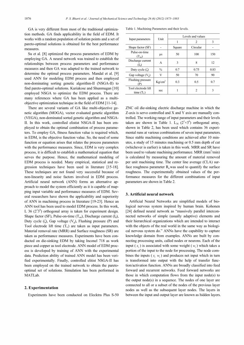
ZNC oil die-sinking electric discharge machine in which the Z-axis is servo controlled and X and Y axis are manually con-trolled. The working range of input parameters and their levels taken are shown in Table 1. L36 (21×36) orthogonal array, shown in Table 2, has been used which contains 36 experi-mental runs at various combinations of seven input parameters. Since stable machining conditions are achieved after 10 min-utes, a study of 15 minutes machining or 0.5 mm depth of cut (whichever is earlier) is taken in this work. MRR and SR have been used to valuate machining performance. MRR (mm3/min) is calculated by measuring the amount of material removed per unit machining time. The center line average (CLA) sur-face roughness parameter Ra was used to quantify the surface roughness. The experimentally obtained values of the per-formance measures for the different combinations of input parameters are shown in Table 2.

3. Artificial neural network

Artificial Neural Networks are simplified models of bio-logical nervous system inspired by human brain. Kohonen [24] defined neural network as “massively parallel intercon-nected networks of simple (usually adaptive) elements and their hierarchical organizations which are intended to interact with the objects of the real world in the same way as biologi-cal nervous system do.” ANNs have the capability to capture knowledge domain from examples. ANNs are built by con-necting processing units, called nodes or neurons. Each of the input ( ix ) is associated with some weight ( iw ) which takes a portion of the input to the node for processing. The node com-bines the inputs ( ix iw ) and produces net input which in turn is transformed into output with the help of transfer func-tion/activation function. ANNs are broadly classified into feed forward and recurrent networks. Feed forward networks are those in which computation flows from the input node(s) to the output node(s) in a sequence. The nodes of one layer are connected to all or a subset of the nodes of the previous layer nodes as well as the subsequent layer nodes. The layers in between the input and output layer are known as hidden layers.

Table 1. Machining Parameters and their levels.

Levels and values Input parameters Unit

1 2 3

Shape factor (SF) - Square Circular - Pulse-on-time

(Ton) µs 50 100 150

Discharge current (Id)

A 3 8 12

Duty cycle (ζ) % 0.7 0.75 0.83

Gap voltage (Vg) V 50 70 90 Flushing pressure

(P) Kg/cm2 0.3 0.5 0.7

Tool electrode lift time (TL) sec 1 2 3

P. S. Bharti et al. / Journal of Mechanical Science and Technology 26 (6) (2012) 1875~1883 1877

In a recurrent network, signals may propagate from the output of any neuron to the input of any neuron. Primarily there are two types of learning methods- supervised and unsupervised learning. In supervised learning method, every input pattern that is used to train the network is associated with an output pattern (i.e. the target or desired pattern). A teacher is assumed to be present during the learning process to determine the error after comparing the network’s computed output and desired output. This error is used to change network parameters which results in improvement in performance. In unsupervised learn-ing method, the system learns by its own by discovering and adapting to structural features in the input pattern in the ab-sence of a teacher. Back propagation (BP) algorithm is one of the most studied and used algorithm for neural networks train-ing. BP neural networks applies the error-back procedure for learning. The back-propagation procedure uses a gradient descent method, which adjusts the weight in its original and simplest form by an amount proportional to the partial deriva-tive of the error function (E) with respect to the given weight.

The formula used for the adjustment (at the tth iteration of the training algorithm) is:

( 1) ( ) .ij ijij

Ew t w t ww

η μ∂+ = − + Δ∂

(1)

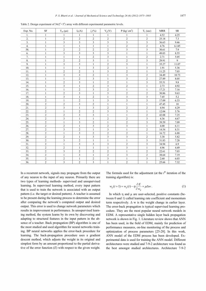
In which η and µ are user-selected, positive constants (be-tween 0 and 1) called learning rate coefficient and momentum term respectively. Δ w is the weight change in earlier layer. The error-back propagation is typical supervised learning pro-cedure. They are the most popular neural network models in EDM. A representative single hidden layer back propagation network is shown in Fig. 1. Literature review shows that ANN has been used, in the field of EDM, mainly for prediction of performance measures, on-line monitoring of the process and optimization of process parameters [25-28]. In this work, ANN model of the EDM process has been developed. Ex-perimental data is used for training the ANN model. Different architectures were studied and 7-9-2 architecture was found as the best amongst studied architectures. Architecture 7-9-2

Table 2. Design experiment of 36(21×36) array with different experimental parametric levels.

Exp. No. SF Ton (μs) Id (A) ζ (%) Vg (V) P (kg/ cm2) TL (sec) MRR SR 1. 1 1 1 1 1 1 1 4.52 4.25 2. 1 2 2 2 2 2 2 25.18 7.3 3. 1 3 3 3 3 3 3 36.63 9.46 4. 1 1 1 1 1 2 2 4.76 6.145 58. 1 2 2 2 2 3 3 30.61 7.9 6. 1 3 3 3 3 1 1 49.03 8.55 7. 1 1 1 2 3 1 2 2.71 5.05 8. 1 2 2 3 1 2 3 29.91 9 9. 1 3 3 1 2 3 1 35.27 11.07 10. 1 1 1 3 2 1 3 1.91 5.36 11. 1 2 2 1 3 2 1 11.25 7.03 12. 1 3 3 2 1 3 2 34.49 10.73 13. 1 1 2 3 1 3 2 27.89 8.05 14. 1 2 3 1 2 1 3 55.51 9.8 15. 1 3 1 2 3 2 1 2.73 4.92 16. 1 1 2 3 2 1 1 17.21 7.16 17. 1 2 3 1 3 2 2 30.86 9.63 18. 1 3 1 2 1 3 3 7.45 5.2 19. 2 1 2 1 3 3 3 17.09 6.33 20. 2 2 3 2 1 1 1 47.45 10 21. 2 3 1 3 2 2 2 4.94 4.29 22. 2 1 2 2 3 3 1 12.04 5.76 23. 2 2 3 3 1 1 2 42.08 7.25 24. 2 3 1 1 2 2 3 4.36 4.67 25. 2 1 3 2 1 2 3 39.59 7.09 26. 2 2 1 3 2 3 1 4.00 6.11 27. 2 3 2 1 3 1 2 14.54 8.31 28. 2 1 3 2 2 2 1 16.72 6.88 29. 2 2 1 3 3 3 2 3.38 5.82 30. 2 3 2 1 1 1 3 31.83 7.28 31. 2 1 3 3 3 2 3 34.94 6.9 32. 2 2 1 1 1 3 1 4.96 4.49 33. 2 3 2 2 2 1 2 22.61 7.03 34. 2 1 3 1 2 3 2 38.64 7.19 35. 2 2 1 2 3 1 3 2.60 6.03 36. 2 3 2 3 1 2 1 25.66 7.32


denotes the number of nodes in input, hidden and output layer. Since the operating ranges of the parameters are different, scal-ing or normalization helps in avoiding skewing the results by any particular variable significantly during training. Input data is scaled (or normalized) between -1 to 1, while the output data is scaled between 0 to 1 to impose the condition of positivity on the output (irrespective of the error of modeling). The values of learning rate coefficient and momentum term have been taken as 0.4 and 0.1 respectively. Several algorithms have been used and the best results were obtained using Bayesian regularization (BR) algorithm. Log-sigmoid activation function has been used for both the layers (hidden and the output layers). For testing the prediction ability of the model, prediction error in each output node has been calculated as follows:

( )(%) *100 .actual value predicted valueprediction error

actual value−=

(2) This prediction error is calculated as absolute percentage er-

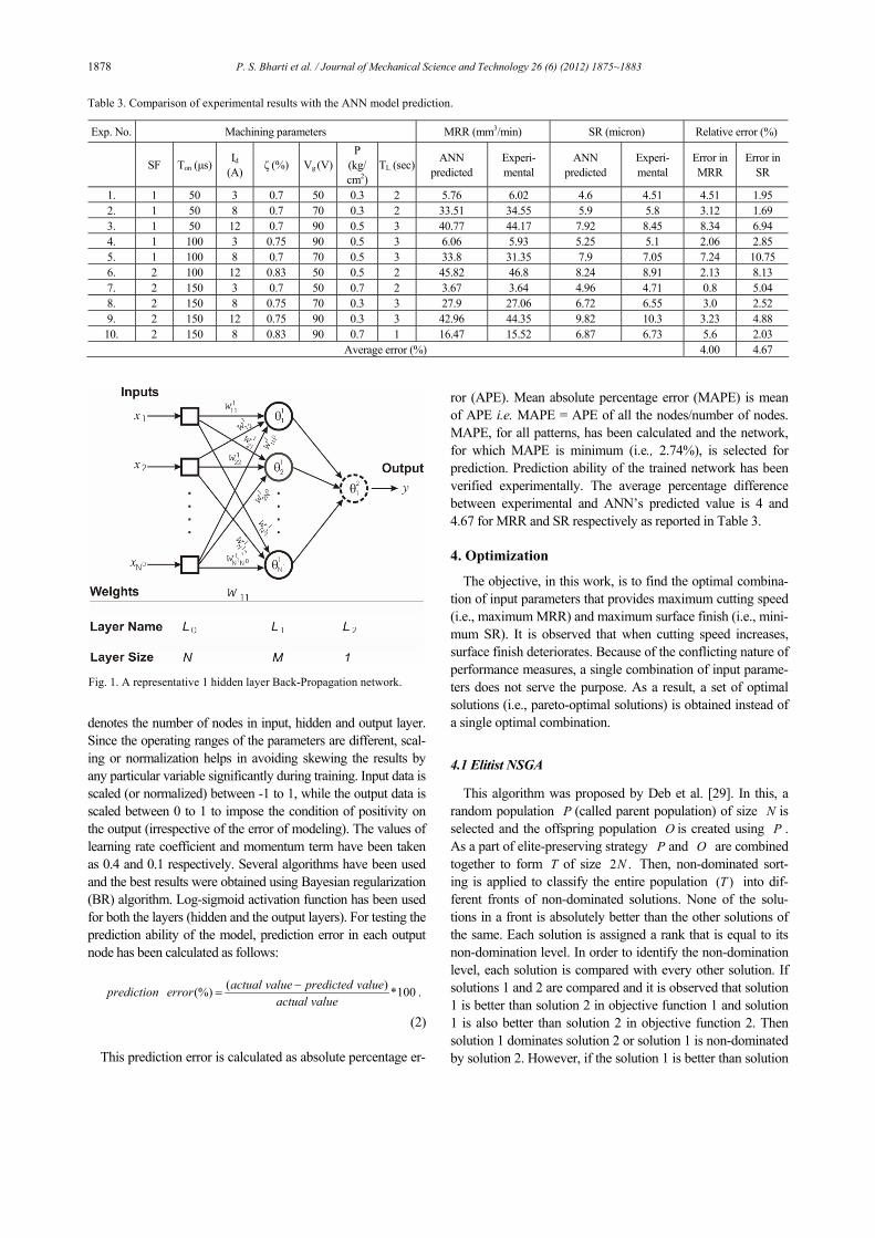
ror (APE). Mean absolute percentage error (MAPE) is mean of APE i.e. MAPE = APE of all the nodes/number of nodes. MAPE, for all patterns, has been calculated and the network, for which MAPE is minimum (i.e., 2.74%), is selected for prediction. Prediction ability of the trained network has been verified experimentally. The average percentage difference between experimental and ANN’s predicted value is 4 and 4.67 for MRR and SR respectively as reported in Table 3.

4. Optimization

The objective, in this work, is to find the optimal combina-tion of input parameters that provides maximum cutting speed (i.e., maximum MRR) and maximum surface finish (i.e., mini-mum SR). It is observed that when cutting speed increases, surface finish deteriorates. Because of the conflicting nature of performance measures, a single combination of input parame-ters does not serve the purpose. As a result, a set of optimal solutions (i.e., pareto-optimal solutions) is obtained instead of a single optimal combination.

4.1 Elitist NSGA

This algorithm was proposed by Deb et al. [29]. In this, a random population P (called parent population) of size N is selected and the offspring population O is created using P . As a part of elite-preserving strategy P and O are combined together to form T of size 2 .N Then, non-dominated sort-ing is applied to classify the entire population ( )T into dif-ferent fronts of non-dominated solutions. None of the solu-tions in a front is absolutely better than the other solutions of the same. Each solution is assigned a rank that is equal to its non-domination level. In order to identify the non-domination level, each solution is compared with every other solution. If solutions 1 and 2 are compared and it is observed that solution 1 is better than solution 2 in objective function 1 and solution 1 is also better than solution 2 in objective function 2. Then solution 1 dominates solution 2 or solution 1 is non-dominated by solution 2. However, if the solution 1 is better than solution

Table 3. Comparison of experimental results with the ANN model prediction. Exp. No. Machining parameters MRR (mm3/min) SR (micron) Relative error (%)

SF Ton (μs) Id

(A) ζ (%) Vg (V) P

(kg/ cm2)

TL (sec) ANN predicted

Experi- mental

ANN predicted

Experi- mental

Error in MRR

Error inSR

1. 1 50 3 0.7 50 0.3 2 5.76 6.02 4.6 4.51 4.51 1.95 2. 1 50 8 0.7 70 0.3 2 33.51 34.55 5.9 5.8 3.12 1.69 3. 1 50 12 0.7 90 0.5 3 40.77 44.17 7.92 8.45 8.34 6.94 4. 1 100 3 0.75 90 0.5 3 6.06 5.93 5.25 5.1 2.06 2.85 5. 1 100 8 0.7 70 0.5 3 33.8 31.35 7.9 7.05 7.24 10.75 6. 2 100 12 0.83 50 0.5 2 45.82 46.8 8.24 8.91 2.13 8.13 7. 2 150 3 0.7 50 0.7 2 3.67 3.64 4.96 4.71 0.8 5.04 8. 2 150 8 0.75 70 0.3 3 27.9 27.06 6.72 6.55 3.0 2.52 9. 2 150 12 0.75 90 0.3 3 42.96 44.35 9.82 10.3 3.23 4.88 10. 2 150 8 0.83 90 0.7 1 16.47 15.52 6.87 6.73 5.6 2.03

Average error (%) 4.00 4.67

Fig. 1. A representative 1 hidden layer Back-Propagation network.


2 in objective function 1, but solution 1 is worse than solution 2 in objective function 2, solution 1 is dominated by solution 2. The concept of dominance and approach used to obtain the pareto-optimal set is mathematically explained as below [30]:

( )1x is said to dominate the other solution ( )2x , if both the conditions 1 and 2 are true:

1. The solution ( )1x is no worse than ( )2x in all objectives, or ( )( ) ( )( )1 2

j jf x f x/ , for all 1,2,......, .j M= i j implies that solution i is worse than solution j on a particular ob-jective.

2. The solution ( )1x is strictly better than ( )2x in at least one objective, or ( )( ) ( )( )1 2

j jf x f x for at least one { }1, 2,........j M∈ . i j implies that solution i is better

than solution j on a particular objective. To provide the diversity in the new population (of size N ),

crowded tournament selection operator is used to fill N solu-tions in the new population. Any of the following condition is true to fill the new population of size N:

1. If solution i has a better rank, that is, ir < jr 2. If they have same rank but solution i has a better crowd-

ing distance than solution j , that is ir = jr and id > jd , where d is the local crowding distance.

Crowding distance is the distance between neighboring so-lutions. The solution lying in the less crowded area, will have larger crowding distance and so is selected. The crowd sorting of the solution of each front is performed by using a crowding distance metric.

4.2 Controlled elitist NSGA-II

It may happen that in a generation, we have a population (to fill N ) where most of the members lie on the non-dominated front of rank one and this front is distant from true pareto-optimal front. The elitism operators will select the members of the non-dominated front of rank one and members of the other fronts will be deleted. As a result, diversity is lost and the so-lutions obtained are not true pareto-optimal solutions.

To counteract this, Deb and Goel [31] proposed a controlled elitist NSGA-II which restricts the number of individuals in the currently best non-dominated front adaptively. In this, each solution is assigned rank in the same manner as it is ap-plied in elitist NSGA-II (as discussed in the previous section). To provide diversity in the population in the new population of size N , the maximum number of individual allowed in the

thi front is restricted and generally given by the following relation:

11

1i

i Frn N r

r−−=

− (3)

where r is reduction rate, a user-defined value, that is less than 1 and F is the number of non-dominated fronts. The strategy employed here forcible allows the solutions from all non-dominated fronts to co-exist in the population. If a par-ticular front is having more solutions than required (to fill N ),

Eq. (3) is used to restrict the number of solutions taken from the concerned front. And if the number of solutions (in a par-ticular front) is less than required (to fill N ), the difference is added in the maximum allowed solutions in the next front and so on. After filling N solutions in the new population, the same process is repeated over a number of generations and the pareto-optimal solutions are obtained. Since the solutions from all non-dominated fronts co-exist in the population, the diversity is maintained and the solutions obtained are true optimal solutions.

To solve optimization problem using GA, fitness value is required. Fitness values, in fact, are the objective function values. In this work, ANN model has been developed to estab-lish the relation between input and output. The objective func-tion values are obtained by the trained network.

5. Results and discussions

The present work aims to maximize MRR and minimize SR. Since the objectives are conflicting in nature, modification of first objective (MRR) is done to get it converted for minimiza-tion. The objective functions are given below:

11Objective

MRR=

2 .Objective SR= Initially, a population of 1000 size has been chosen. The

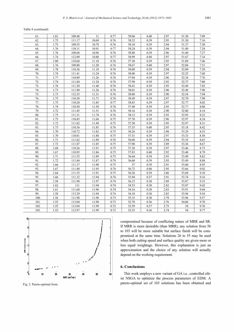
values of the objective functions are obtained from trained network. Trained network provides the function which relates the input parameters with the performance measures. Pareto fraction is taken as 0.1. For better convergence, 500 genera-tions are taken in this work. One hundred three non-dominated solutions (pareto-optimal solutions) are obtained at the end of 500 generations. The pareto-optimal solutions (along with corresponding performance measure values) are reported in Table 4. Fig. 2 shows the formation of pareto-optimal front that consists the final set of solutions. The shape of the pareto optimal front is a consequence of the continuous nature of the optimization problem posed. The results reported in Table 4 clearly show that in 103 pareto-optimal solutions, the whole given range of input parameters is reflected and no bias to-wards higher side or lower side of the parameters is seen. This may be attributed to the controlled NSGA that forcible allows the solutions from all non-dominated fronts to co-exist in the population. Since the performance measures are conflicting in nature, surface quality decreases as MRR increases and the same behavior of performance measures is observed in the solutions obtained. Since none of the solutions in the pareto-optimal set is absolutely better than any other, any one of them is an acceptable solution. The choice of one solution over the other depends on the requirement of the process engineer. If surface finish is more desirable (than SR), any solution from 1 to 25 will be more suitable. But at the same time MRR will be


Table 4. Pareto-optimal solutions.

Solution No. SF Ton (μs) Id (A) ζ (%) Vg (V) P (kg/ cm2) TL (sec) MRR SR 1. 1.79 117.42 3 0.79 55.19 0.31 1.88 4.67 4.33 2. 1.80 118.47 3 0.79 55.09 0.32 1.92 4.67 4.33 3. 1.75 117.66 3 0.79 55.12 0.32 1.87 4.83 4.33 4. 1.77 117.70 3 0.79 55.19 0.33 1.94 4.94 4.33 5. 1.74 118.75 3 0.78 55.32 0.35 1.92 5.15 4.33 6. 1.74 118.06 3.14 0.78 54.76 0.34 1.91 5.27 4.33 7. 1.74 119.76 3.50 0.79 55.44 0.34 1.96 5.81 4.34 8. 1.72 121.80 3.31 0.78 57.12 0.36 2.17 6.09 4.35 9. 1.71 120.94 3.41 0.78 54.97 0.35 2.15 6.39 4.35 10. 1.73 117.52 3.60 0.77 54.67 0.34 2 6.61 4.35 11. 1.71 122.90 3.80 0.78 55.50 0.34 2 6.82 4.36 12. 1.73 119.65 3.69 0.77 56.12 0.34 2.18 6.95 4.36 13. 1.68 120.24 3.80 0.77 55.37 0.33 2.21 7.37 4.36 14. 1.74 117 3.82 0.77 56.00 0.34 2.29 7.56 4.37 15. 1.76 120.93 4.18 0.78 55.90 0.36 2.14 8.01 4.38 16. 1.72 118.91 4.08 0.77 55.84 0.35 2.21 8.23 4.38 17. 1.73 124.29 4.23 0.77 56.18 0.35 2.20 8.72 4.38 18. 1.74 114.57 4.79 0.79 55.86 0.34 2.11 9.48 4.41 19. 1.74 114.73 4.83 0.79 55.59 0.34 2.07 9.66 4.41 20. 1.69 116.36 4.75 0.77 55.09 0.32 2.13 10.23 4.41 21. 1.65 120.38 4.82 0.76 54.82 0.35 2.44 13.12 4.46 22. 1.73 116.31 5.40 0.77 56.15 0.34 2.20 13.86 4.48 23. 1.75 115.39 5.75 0.77 55.59 0.35 2.34 17.40 4.55 24. 1.73 117.31 5.94 0.77 56.62 0.37 2.67 19.18 4.60 25. 1.77 112.42 6.26 0.77 56.16 0.35 2.86 21.28 4.64 26. 1.62 138.69 8.36 0.82 85.71 0.35 1.75 35.19 4.94 27. 1.59 138.24 8.49 0.83 86.22 0.36 1.66 36.84 5.01 28. 1.65 139.00 9.13 0.83 86.31 0.38 1.81 40.01 5.15 29. 1.64 139 9.47 0.83 86.88 0.35 1.66 42.01 5.20 30. 1.57 139.11 9.87 0.83 85.93 0.34 1.64 43.77 5.35 31. 1.63 139.17 10.20 0.83 86.89 0.33 1.65 44.69 5.38 32. 1.54 139.53 10.23 0.83 86.72 0.34 1.68 45.06 5.47 33. 1.63 139.40 10.28 0.83 85.42 0.36 1.71 45.11 5.52 34. 1.55 139.49 10.57 0.83 86.66 0.34 1.64 46.20 5.61 35. 1.63 139.42 10.79 0.83 86.63 0.36 1.77 46.38 5.63 36. 1.53 139 10.70 0.82 86.31 0.34 1.72 46.48 5.69 37. 1.57 138.83 10.96 0.82 86.84 0.34 1.68 47.10 5.74 38. 1.50 139.81 10.91 0.83 86.78 0.33 1.64 47.18 5.81 39. 1.60 137.25 11.75 0.83 86.89 0.33 2.02 48.05 5.89 40. 1.50 139.95 11.29 0.83 86.90 0.33 1.60 48.13 5.98 41. 1.60 136.25 11.81 0.83 86.96 0.38 1.83 48.43 6.04 42. 1.56 140 11.65 0.83 86.78 0.33 1.66 48.71 6.09 43. 1.52 138.69 11.72 0.82 86.67 0.33 1.75 48.76 6.15 44. 1.53 139.92 11.74 0.83 86.92 0.34 1.70 48.88 6.17 45. 1.49 140.17 11.67 0.83 86.88 0.33 1.59 48.92 6.23 46. 1.49 140.17 11.67 0.83 86.88 0.33 1.58 48.93 6.24 47. 1.49 140.16 11.76 0.83 86.92 0.32 1.58 49.13 6.30 48. 1.49 140.16 11.76 0.83 86.92 0.32 1.58 49.15 6.31 49. 1.86 108.01 10.36 0.77 59.95 0.41 3.00 49.20 6.38 50. 1.76 109.50 10.01 0.76 59.27 0.39 2.95 49.26 6.43 51. 1.86 108.82 10.41 0.77 59.45 0.40 2.98 49.51 6.46 52. 1.77 110.23 10.01 0.77 58.35 0.40 2.89 49.54 6.55 53. 1.77 110.24 10.19 0.77 58.69 0.39 2.94 49.70 6.56 54. 1.74 110.61 10 0.76 58.95 0.40 2.94 49.84 6.61 55. 1.75 111.23 10.23 0.77 58.63 0.40 2.93 49.86 6.67 56. 1.77 110.10 10.16 0.76 58.10 0.40 2.91 50.06 6.70 57. 1.74 110.57 10.21 0.76 58.45 0.39 2.91 50.22 6.75 58. 1.79 109.87 10.64 0.76 57.96 0.39 2.98 50.75 6.89 59. 1.76 110.87 10.40 0.76 58.13 0.39 2.91 50.75 6.96 60. 1.81 108.06 11.08 0.77 59.16 0.39 2.95 51.10 7.04


Table 4 (continued)

61. 1.81 109.48 11 0.77 59.06 0.40 2.97 51.30 7.09 62. 1.75 111.17 10.69 0.76 58.32 0.39 2.95 51.30 7.16 63. 1.75 109.55 10.78 0.76 58.10 0.39 2.94 51.37 7.20 64. 1.76 110.11 10.91 0.77 58.24 0.39 2.94 51.49 7.24 65. 1.76 109.68 10.96 0.76 58.80 0.39 2.96 51.60 7.27 66. 1.74 112.09 10.88 0.77 58.99 0.40 2.97 51.67 7.34 67. 1.80 110.68 11.18 0.76 57.30 0.39 2.95 51.89 7.46 68. 1.76 109.80 11.20 0.76 58.67 0.40 2.97 52.04 7.51 69. 1.78 110.36 11.18 0.76 58.09 0.39 2.94 52.09 7.59 70. 1.74 111.41 11.24 0.76 58.00 0.39 2.97 52.25 7.68 71. 1.77 110.89 11.26 0.76 57.04 0.39 2.96 52.34 7.76 72. 1.74 111.84 11.24 0.76 57.99 0.39 2.92 52.37 7.80 73. 1.76 111.20 11.48 0.76 58.41 0.39 2.95 52.49 7.82 74. 1.73 111.90 11.26 0.76 58.01 0.39 2.90 52.49 7.90 75. 1.73 112.35 11.31 0.76 58.80 0.39 2.90 52.54 7.94 76. 1.75 110.38 11.71 0.76 58.49 0.39 2.97 52.70 7.98 77. 1.75 110.20 11.85 0.77 58.83 0.39 2.97 52.77 8.02 78. 1.74 110.50 11.50 0.76 57.40 0.39 2.95 52.77 8.08 79. 1.72 111.45 11.51 0.76 58.16 0.38 2.90 52.80 8.14 80. 1.75 111.31 11.74 0.76 58.13 0.39 2.93 52.95 8.22 81. 1.75 110.45 11.66 0.75 57.70 0.39 2.96 52.97 8.24 82. 1.72 111.82 11.49 0.75 57.50 0.39 2.95 52.97 8.31 83. 1.73 110.36 11.85 0.76 57.53 0.40 2.95 53.18 8.42 84. 1.70 110.72 11.82 0.75 58.26 0.39 2.98 53.29 8.53 85. 1.70 110.81 11.80 0.75 57.51 0.39 2.97 53.33 8.58 86. 1.71 111.62 11.89 0.76 56.68 0.39 2.94 53.35 8.63 87. 1.72 111.87 11.85 0.75 57.90 0.39 2.89 53.36 8.67 88. 1.68 110.26 11.91 0.75 57.28 0.39 2.97 53.46 8.73 89. 1.67 110.95 11.86 0.75 57.83 0.40 2.92 53.48 8.79 90. 1.71 111.55 11.89 0.75 56.64 0.38 2.93 53.49 8.82 91. 1.72 111.84 11.87 0.74 56.60 0.39 2.93 53.49 8.88 92. 1.66 111.37 11.90 0.75 57 0.39 2.91 53.60 8.95 93. 1.67 111.48 11.95 0.74 56.72 0.40 2.95 53.66 9.02 94. 1.64 111.35 11.91 0.75 56.26 0.39 2.86 53.68 9.10 95. 1.66 111.32 11.94 0.74 53.94 0.37 2.91 53.74 9.16 96. 1.58 111.98 11.97 0.74 56.15 0.38 2.89 53.87 9.33 97. 1.62 111 11.94 0.74 54.53 0.38 2.82 53.87 9.42 98. 1.61 111.68 11.96 0.74 54.16 0.38 2.83 53.91 9.44 99. 1.58 113.29 11.94 0.74 54.10 0.38 2.82 53.94 9.54 100. 1.56 111.98 11.98 0.73 55.33 0.38 2.79 53.96 9.57 101. 1.55 113.04 11.98 0.73 52.70 0.36 2.76 54.06 9.70 102. 1.55 113.04 11.99 0.72 52.59 0.37 2.75 54 9.76 103. 1.52 112.97 11.99 0.72 52.53 0.36 2.74 54 9.77

compromised because of conflicting nature of MRR and SR. If MRR is more desirable (than MRR), any solution from 56 to 103 will be more suitable but surface finish will be com-promised at the same time. Solutions 26 to 55 may be used when both cutting speed and surface quality are given more or less equal weightage. However, this explanation is just an approximation and the choice of any solution will actually depend on the working requirement.

6. Conclusions

This work employs a new variant of GA i.e., controlled elit-ist NSGA to optimize the process parameters of EDM. A pareto-optimal set of 103 solutions has been obtained and

Fig. 2. Pareto-optimal front.


reported by employing controlled elitist NSGA. The solutions obtained are true representation of the given range of the input parameters and are not biased. This asserts the fact that con-trolled elitist NSGA controls elitism and forcibly allows the solutions from each non-dominating front to co-exist in the population. This leads to true optimal solutions. Fitness value (i.e., objective function in case of EDM) has been obtained by developing the neural network model of EDM process. For this, a large number of experiments were conducted on die-sinking EDM with a wide range of input parameters. The per-formance measures were measured for each combination of input parameters. A feed forward back-propagation neural network was used to model the EDM process. Experimental data was used to train neural network. Various ANN architec-tures were studied and 7-9-2 architecture was found as the best amongst studied architectures. The corresponding MAPE was as low as 2.74. The prediction ability of the trained network has been verified experimentally. The average percentage difference between experimental and ANN’s predicted value is 4 and 4.67 for MRR and SR respectively.

Acknowledgement

The authors are thankful to Dr. Pravin Chandra of Institute of Informatics and Communications, University of Delhi, South Campus, Delhi (India) for his valuable suggestions in neural network and help in simulation work.

References

[1] J. A. McGeough, Advanced methods of machining, Chap-man & Hall, London (1998).

[2] S. Kirkpatric, C. Gelatt and M. Vecchi, Optimization by simulated annealing, Science, 220 (1983) 4598.

[3] Y. S. Tarng, S. C. Ma and L. K. Chung, Determination of optimal cutting parameters in wire electrical discharge ma-chining, Int. J. of Mach. Tools Manuf., 35 (1995) 1693-1701.

[4] S. H. Yang, J. Srinivas, S. Mohan, D. M. Lee and S. Balaji, Optimization of electric discharge machining using simu-lated annealing, J. Mater. Process. Technol., 209 (2009) 4471-4475.

[5] J. T. Huang and Y. S. Liao, Optimization of machining of wire-EDM based on Grey relational and statistical analyses, Int. J. Prod. Research, 41 (2003) 1707-1720.

[6] C. L. Lin, J. L. Lin and T. C. Ko, Optimization of EDM process based on the orthogonal array with fuzzy logic and grey relational analysis method, Int. J. Adv. Manuf. Technol., 19 (2002) 271-277.

[7] J. H. Jung and W. T. Kwon, Optimization of EDM process for multiple performance characteristics using Taguchi method and Grey relational analysis, J. Mech. Sc. Tech., 24 (5) (2010) 1083-1090.

[8] J. C. Su, J. Y. Kao and Y. S. Tarng, Optimization of the electrical discharge machining process using a GA-based

neural network, Int. J. Adv. Manuf. Technol., 24 (2004) 81-90.

[9] D. Mandal, S. K Pal and P. Saha, Modeling of electric dis-charge machining process using back propagation neural network and multi-objective optimization using non-dominating sorting genetic algorithm-II, J. Mat. Process. Technol., 186 (2007) 154-162.

[10] S. Kuriakose and M. S. Shunmugan, Multi-objective opti-mization of wire-electro discharge machining process by Non-Dominated Sorting genetic algorithm, J. Mat. Process. Technol., 170 (2005) 133-141.

[11] G. K. M. Rao, G. Rangajanardhaa, D. H. Rao and M. S. Rao, Development of hybrid model and optimization of sur-face roughness in electric discharge machining using artifi-cial neural networks and genetic algorithm, J. Mat. Process. Technol., 209 (2009) 1512-1520.

[12] N. K. Jain, V. K. Jain and K. Deb, Optimization of process parameters of mechanical type advanced machining proc-esses using genetic algorithms, Int. J. Mach. Tools Manuf., 47 (2007) 900-919.

[13] A. Dev, K. M. Patel, S. Pandey and S. Aravindan, Machin-ing charactersistics and optimization of process parameters in micro-EDM of SiCp-Al composites, Int. J. Manuf. Re-search, 4 (4) (2009) 458-480.

[14] C. Fenggou and Y. Dayong, The study of high efficiency and intelligent optimization system in EDM sinking process, J. Mat. Process. Technol., 149 (2004) 83-87.

[15] N. Tosun, The effect of cutting parameters on performance of WEDM, K.S.M.E. Int. J., 17 (6) (2003) 816-824.

[16] J. C. Rebelo, A. M. Dias, R. Mesquita, P. Vassalo and M. Santos, An experimental study on electro-discharge machin-ing and polishing of high strength copper-berrylium alloys, J. Mat. Process. Technol., 103 (2000) 389-397.

[17] G. Petropoulos, N. M. Vaxevanidis and C. Pandazaras, Modeling of surface finish in electro-discharge machining based on statistical multi-parameter analysis J. Mat. Process. Technol.,155-156 (2004) 1247-1251.

[18] H. Zorepour, A. F. Tehrani, D. Karimi and S. Amini, Statis-tical analysis on electrode wear in EDM of tool steel DIN 1.2714 used in forging dies, J. Mat. Process. Technol., 187-188 (2007) 711-714.

[19] T. A. Speeding and Z. Q. Wang, Parametric optimization and surface characterization of wire electrical discharge ma-chining process, Precision Engineering, 20 (1997) 5-15.

[20] W. Sukthmoya and J. Tannock, The training of neural net-works to model manufacturing processes, J. Intelligent Manuf., 16 (2005) 39-51.

[21] S. Assarzadeh and M. Ghoresishi, Neural-network based modeling and optimization of the electro-discharge ma-chining process, Int. J. Adv. Manuf. Technol, 39 (2008) 488-500.

[22] V. S. Sharma, S. Dhiman, R. Sehgal and S. K. Sharma, Estimation of cutting forces and surface roughness for hard turning using neural network, J. Intelligent Manuf., 19 (2008) 473-483.


[23] C. Lucignano, R. Montanari, V. Tagliaferri and N. Ucci-ardello, Artificial neural network to optimize the extrusion of an aluminum alloy, J. Intelligent Manuf., 21 (2009) 569-574.

[24] T. Kohonen, Adaptive and associative, and self-organization functions in neural computing, Applied Optics, 26 (1987) 4910-4918.

[25] J. Y. Kao and Y. S. Tarng, A neural network approach for the on-line monitoring of electric discharge machining proc-ess, J. Mat. Process. Technol., 69 (1997) 112-119.

[26] D. K. Panda and R. K. Bhoi, Artificial neural network prediction of material removal rate in electro-discharge machining, Mat. and Manuf. Process., 20 (4) (2005) 645-672.

[27] A. P. Markopoulos, D. E. Manolakos and N. M. Vaxevani-dis, Artificial neural network models for the prediction of surface roughness in electrical discharge machining, J. Intel-ligent Manuf., 19 (2008) 283-292.

[28] K. M. Tsai and P. J. Wang, Comparisons of neural network models on material removal rate in electric discharge ma-chining, J. Mat. Process. Technol., 117 (2001) 111-124.

[29] K. Deb, S. Aggarwal, A. Pratap and T. Meyarivan, A fast elitist non-dominated sorting genetic algorithm for multi-objective optimization:NSGA-II, Proc. of the parallel prob-lem solving from nature, VI(PPSN-VI) (2000) 849-858.

[30] K. Deb, Multi-objective optimization using evolutionary algorithms, John Wiley & Sons (ASIA) Pte Ltd, Singapore (2003).

[31] K. Deb, T. Goel, Controlled elitist non-dominated sorting genetic algorithms for better convergence, Proc. of the first international conference on evolutionary multi-criterion optimization, Springer, Berlin (2001) 67-81.

Pushpendra S. Bharti received his B.Sc. Engg. in Mechanical Engineering from D.E.I. Agra, India. He did his M.E. in production engineering from Motilal National Institute of Technology, Alla-habad, India. He is working with G.G.S.Indraprastha University, Delhi, India as Assistant Professor. He has

submitted his Ph.D thesis on optimization of process parame-ters of EDM. His research area includes non-conventional machining and manufacturing automation.

Sachin Maheshwari is working as Pro-fessor & Head, MPAE division, Netaji Subhas Institute of Technology, Delhi, India. He received his Ph.D from Indian Institute of Technology, Delhi and M.Tech. from Indian Institute of Tech-nology, Roorkee, India after graduating from Motilal Nehru National Institute of

Technology, Allahabad, India. His current research interest includes conventional, non-conventional, hybrid manufactur-ing processes and manufacturing automation.

Chitra Sharma is Associate Professor and Head at Department of MAE, Indira Gan-dhi Institute of Technology, Delhi, India. She received her Ph.D from Indian Institute of Technology, Delhi. India. Her current research interest include conventional, non-conventional manufacturing processes, computer aided manufacturing.

Multi-objective optimization of electric-discharge ...

Documents

Transcript of Multi-objective optimization of electric-discharge ...