Multi-Objective Decision-Theoretic Planningroijers.info/pub/thesis.pdf · op gezag van de Rector...
171
Multi-Objective Decision-Theoretic Planning Diederik M. Roijers
Transcript of Multi-Objective Decision-Theoretic Planningroijers.info/pub/thesis.pdf · op gezag van de Rector...

Multi-Objective Decision-TheoreticPlanning
Diederik M. Roijers

ISLA Dissertation
For further information about ISLA-publications, please contact
Intelligent Systems Lab AmsterdamUniversiteit van Amsterdam
Science Park 9041098 XH Amsterdam
phone: +31-20-525-7463homepage: http://isla.science.uva.nl/
The investigations were supported by the DTC-NCAP (#612.001.109) project of theNetherlands Organization for Scientific Research (NWO).
Copyright c© 2016 by Diederik M. RoijersISBN: 978–94–6328–039–6

Multi-Objective Decision-TheoreticPlanning
ACADEMISCH PROEFSCHRIFT
ter verkrijging van de graad van doctor aan deUniversiteit van Amsterdam
op gezag van de Rector Magnificusprof.dr. D.C. van den Boom
ten overstaan van een door het college voorpromoties ingestelde commissie, in het openbaar
te verdedigen in de Agnietenkapelop dinsdag 24 mei 2016, te 10.00 uur
door
Diederik Marijn Roijers
geboren te Nijmegen

Promotor: prof. dr. Max Welling Universiteit van Amsterdam
Co-promotores: dr. Shimon A. Whiteson Universiteit van Amsterdam
dr. Frans A. Oliehoek Universiteit van Amsterdam
Overige leden: prof. dr. Ann Nowe Vrije Universiteit Brussel
prof. dr. Karl Tuyls University of Liverpool
prof. dr. ir. Frans C. A. Groen Universiteit van Amsterdam
dr. Joris M. Mooij Universiteit van Amsterdam
dr. Maarten W. van Someren Universiteit van Amsterdam
Faculteit der Natuurwetenschappen, Wiskunde en Informatica
iii


Contents
Acknowledgments ix
1 Introduction 11.1 Motivating Scenarios . . . . . . . . . . . . . . . . . . . . . . . . . . 21.2 Utility-Based Approach . . . . . . . . . . . . . . . . . . . . . . . . . 61.3 Focus . . . . . . . . . . . . . . . . . . . . . . . . . . . . . . . . . . 71.4 Research Questions . . . . . . . . . . . . . . . . . . . . . . . . . . . 91.5 Contributions and Outline . . . . . . . . . . . . . . . . . . . . . . . . 9
2 Background 132.1 Multiple Objectives . . . . . . . . . . . . . . . . . . . . . . . . . . . 13
2.1.1 Undominated Sets . . . . . . . . . . . . . . . . . . . . . . . 152.1.2 Coverage Sets . . . . . . . . . . . . . . . . . . . . . . . . . . 172.1.3 Approximate Coverage Sets . . . . . . . . . . . . . . . . . . 18
2.2 Overview of Concrete Decision Problems . . . . . . . . . . . . . . . 192.2.1 Bandit Problems . . . . . . . . . . . . . . . . . . . . . . . . 202.2.2 Overview of Decision Problems . . . . . . . . . . . . . . . . 22
2.3 Case for the Convex Coverage Set . . . . . . . . . . . . . . . . . . . 24
3 Optimistic Linear Support 293.1 Inner Loop versus Outer Loop . . . . . . . . . . . . . . . . . . . . . 30
3.1.1 The Inner Loop Approach . . . . . . . . . . . . . . . . . . . 323.1.2 The Outer Loop Approach . . . . . . . . . . . . . . . . . . . 36
3.2 The Scalarized Value Function . . . . . . . . . . . . . . . . . . . . . 373.3 The OLS Algorithm . . . . . . . . . . . . . . . . . . . . . . . . . . . 383.4 Analysis . . . . . . . . . . . . . . . . . . . . . . . . . . . . . . . . . 463.5 Approximate Single-Objective Solvers . . . . . . . . . . . . . . . . . 473.6 Value reuse . . . . . . . . . . . . . . . . . . . . . . . . . . . . . . . 51
v

4 Coordination 534.1 Coordination Graphs . . . . . . . . . . . . . . . . . . . . . . . . . . 54
4.1.1 Variable Elimination . . . . . . . . . . . . . . . . . . . . . . 574.1.2 AND/OR tree search . . . . . . . . . . . . . . . . . . . . . . 604.1.3 Variational methods . . . . . . . . . . . . . . . . . . . . . . 62
4.2 Multi-objective Coordination Graphs . . . . . . . . . . . . . . . . . . 644.3 Inner Loop CCS Methods for MO-CoGs . . . . . . . . . . . . . . . . 65
4.3.1 Convex Multi-Objective Variable Elimination . . . . . . . . . 664.3.2 Experiments: CMOVE versus PMOVE . . . . . . . . . . . . 744.3.3 Convex AND/OR Tree Search . . . . . . . . . . . . . . . . . 794.3.4 Experiments: CTS versus CMOVE . . . . . . . . . . . . . . 81
4.4 OLS for MO-CoGs . . . . . . . . . . . . . . . . . . . . . . . . . . . 844.4.1 Variable Elimination Linear Support . . . . . . . . . . . . . . 844.4.2 Experiments: VELS versus CMOVE . . . . . . . . . . . . . . 854.4.3 AND/OR Tree Search Linear Support . . . . . . . . . . . . . 894.4.4 Experiments: TSLS versus VELS and CTS . . . . . . . . . . 904.4.5 Variational Optimistic Linear Support . . . . . . . . . . . . . 924.4.6 Experiments: VOLS versus VELS . . . . . . . . . . . . . . . 96
4.5 Conclusion . . . . . . . . . . . . . . . . . . . . . . . . . . . . . . . 100
5 Sequential Decision-Making 1035.1 Background . . . . . . . . . . . . . . . . . . . . . . . . . . . . . . . 104
5.1.1 Markov decision processes . . . . . . . . . . . . . . . . . . . 1055.1.2 Partially Observable Markov Decision Problems . . . . . . . 108
5.2 OLS for Large Finite-Horizon MOMDPs . . . . . . . . . . . . . . . 1115.2.1 The Maintenance Planning Problem . . . . . . . . . . . . . . 1115.2.2 Solving MPP instances . . . . . . . . . . . . . . . . . . . . . 1135.2.3 Experiments: MPP . . . . . . . . . . . . . . . . . . . . . . . 115
5.3 OLS with Alpha Reuse for MOPOMDPs . . . . . . . . . . . . . . . . 1175.3.1 Point-based POMDP methods . . . . . . . . . . . . . . . . . 1185.3.2 Optimistic Linear Support with Alpha Reuse . . . . . . . . . 1195.3.3 Experiments: MOPOMDPs . . . . . . . . . . . . . . . . . . 124
5.4 Conclusion . . . . . . . . . . . . . . . . . . . . . . . . . . . . . . . 127
6 Conclusion 1296.1 Contributions . . . . . . . . . . . . . . . . . . . . . . . . . . . . . . 129
6.1.1 The big picture . . . . . . . . . . . . . . . . . . . . . . . . . 1296.1.2 Problem-specific contributions . . . . . . . . . . . . . . . . . 132
6.2 Discussion and Future Work . . . . . . . . . . . . . . . . . . . . . . 1346.2.1 On the sufficiency of the taxonomy . . . . . . . . . . . . . . 1346.2.2 Scalarized expectation of return versus expectation of scalar-
ized return . . . . . . . . . . . . . . . . . . . . . . . . . . . 1356.2.3 Other decision problems . . . . . . . . . . . . . . . . . . . . 137
vi

6.2.4 Other aspects of decision problems . . . . . . . . . . . . . . 1386.2.5 Reuse in OLS and scalability in the number of objectives . . . 1386.2.6 Decision makers in the loop . . . . . . . . . . . . . . . . . . 139
Bibliography 141
Abstract 153
Samenvatting 155
Overview of Publications 157
vii


Acknowledgments
At the end of this four-year journey, I am truly grateful to many people. I will mentionseveral people specifically.
First, I want to thank my supervisors, Shimon and Frans, who taught me morethan I ever thought I could learn. Thank you for your guidance and many interestingdiscussions.
I want to thank my wife, Emi, who accompanied me every step of the way. Notonly did she tolerate my stress levels and long deadline nights, but actually helped methrough them. Also, I want to thank my parents, Marloes and Fred, and my sister,Simone, for their constant support. This dissertation would not have been possiblewithout you.
Thanks also to Joeri, Simone and Julienne, for proofreading and giving me feed-back on my dissertation. Thanks to my co-authors (Peter, Richard, Joris, Dirk, Matthijs,Mathijs, Sander, Guangliang, Alex and Daan). It has been great working with you, andI hope we can do so again.
Special thanks to the students whom I had the pleasure of supervising and teaching(a.o., Chiel, Lieuwe, Sander, Maarten, Maarten, Auke, Camiel, Eugenio, Luisa, Timon,Philipp, Mircea, Paris, Elise, Carla, Marysia, Richard, Edwin, Maarten, and Joost).
Thanks to prof. Ann Nowe and prof. Abdel-Illah Mouaddib, for inviting me toyour labs. These visits were very inspiring. Thanks to John-Jules Meyer, Linda vander Gaag, Silja Renooij, Robby Tan, Johan Jeuring and Ad Feelders, for kindling myinterest in computer science and research, and inspiring me to go and do a PhD. Thanksto my colleagues and friends at the UvA (and across the street at CWI), SIKS, and theAAMAS and wider AI communities. And last but not least, thanks to all my friendsand family who have supported me throughout this journey.
Leiden, Diederik M. Yamamoto-RoijersApril 12, 2016.
ix


Chapter 1Introduction
A central problem in artificial intelligence is the design of artificial autonomous agents.An agent is “anything that can be viewed as perceiving its environment through sen-sors and acting upon that environment through effectors” (Russell et al., 1995), i.e.,an artificial agent typically is a computer program — possibly embedded in specifichardware — that takes actions in an environment that changes as a result of these ac-tions. An autonomous agent (Franklin and Graesser, 1997) can act autonomously, i.e.,without constant human control or intervention, on a user’s behalf.1
Artificial autonomous agents can assist us in many useful ways. For example,agents can perform the control of manufacturing machine, in order to produce productsfor a company (Monostori et al., 2006; Van Moergestel, 2014), drive a car instead of ahuman driver (Guizzo, 2011), trade goods or services on markets (Ketter et al., 2013;Pardoe, 2011) and help provide security (Tambe, 2011). As such, autonomous agentshave enormous economic potential, as well as potential for improving our quality oflife.
In order to perform tasks, autonomous agents require the capacity to reason abouttheir environment and consequences of their actions — and the desirability thereof.The study of this reasoning is called decision theory. Decision theory uses probabilisticmodels of the environment. Typically these models include the states the environmentcan be in, the possible actions that agents can perform in each state, and how the stateof the environment is affected by these actions. Furthermore, the desirability of actionsand their effects are codified in numerical feedback signals. These feedback signals aretypically referred to as reward or payoff functions.
Decision-theoretical models enable autonomous agents to plan how to act. Themodels encode how the environment behaves as a result of the actions agents andwhich observations and rewards agents can expect. Agents can use this informationto formulate a policy that specifies agent behavior as a function of what the agentsobserve.
1For a detailed discussion on the definition of autonomous agents, see e.g., the discourses by Russellet al. (1995) and Franklin and Graesser (1997).
1

2 Chapter 1. Introduction
In most research on planning in decision problems, the desirability of actions andtheir effects are codified in a scalar reward function (Busoniu et al., 2008; Oliehoek,2010; Thiebaux et al., 2006; Wiering and Van Otterlo, 2012). The planning task insuch scenarios is to find a policy that maximizes the expected (cumulative) reward.
However, many real-world decision problems have multiple objectives. For exam-ple, for a computer network we may want to maximize performance while minimizingpower consumption (Tesauro et al., 2007). In such cases the problem is more natu-rally expressed using a vector-valued reward function. When the reward function isvector-valued, the value of a policy is also vector-valued. Typically, there is no singlepolicy that maximizes the value for all objectives simultaneously. For example, in thecomputer network example, we can achieve higher performance by using more power.Rather than producing a single optimal policy, as in single-objective planning, it maytherefore be crucial to produce a set of policies that offer different trade-offs betweenthe objectives.
In this dissertation, we focus on multi-objective decision-theoretic planning. In amulti-objective planning scenario, the agents are given a model of the environmentand asked to provide a set of policies from which to elect a policy to execute. We firstmotivate the need for specialized multi-objective planning methods in this scenario,and introduce our perspective on what it means to solve a multi-objective decisionproblem. Then we introduce the research questions, the scope of this dissertation andprovide an overview of the contributions in this dissertation.
1.1 Motivating ScenariosThe existence of multiple objectives in a decision problem does not automatically im-ply that we require specialized multi-objective methods to solve it. If the decisionproblem can be scalarized, i.e., the vector-valued reward function can be converted toa scalar reward function, the problem may be solvable with existing single-objectivemethods. Such a conversion involves two steps (Roijers et al., 2013a). The first stepis to specify a scalarization function that expresses the utility of the user for differenttrade-offs between the objectives.
Definition 1. A scalarization function f , is a function that maps a multi-objective valueof a policy π of a decision problem, Vπ, to a scalar value V π
w :
V πw = f(Vπ,w),
where w is a so-called weight vector that parameterizes f .
The second step of the conversion is to define a single-objective version of the decisionproblem such that the utility of each policy π equals the scalarized value of the originalmulti-objective decision problem V π
w .Though it is rarely stated explicitly, all research on automated multi-objective deci-
sion making rests on the premise that there are decision problems for which one or both

1.1. Motivating Scenarios 3
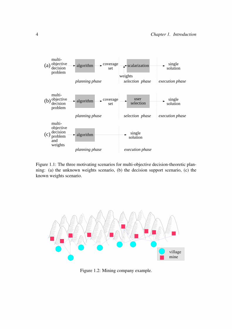
of these conversion steps are impossible, infeasible, or undesirable. Here, we discussthree motivating scenarios in which this is indeed the case, thereby demonstrating theneed for specialized multi-objective methods. These scenarios are depicted schemati-cally in Figure 1.1.
Figure 1.1a provides an overview of the unknown weights scenario. In this sce-nario, w is unknown at the moment when planning must occur: the planning phase.For example, consider a company that mines different resources from different minesspread out through a mountain belt. The workers of the company live in villages atthe foot of the mountains. In Figure 1.2, we depict the problem this company faces:in the morning one van per village needs to transport workers from that village to anearby mine, where various resources can be mined. Different mines yield differentquantities of resource per worker. The market prices per unit of resource vary througha stochastic process and every price change can change the optimal assignment ofvans. Furthermore, the expected price variation increases with time. It is thereforecritical to act based on the latest possible price information in order to maximize per-formance. Because computing the optimal van assignment takes time, redoing thiscomputation every time the prices change is highly undesirable. Therefore, we needa multi-objective method that computes a set containing an optimal solution for everypossible value of the prices, w. We call such a set a coverage set, as it “covers” allpossible preferences of the user (i.e., the possible values of the prices in our example)with respect to the objectives (as specified by f ). Although computing a coverage setis computationally more expensive than computing a single optimal policy for a givenprice, it needs to be done only once. Furthermore, the planning phase (Figure 1.1a)can take place in advance, when more computational resources are available.
In the selection phase, when the prices (w) are revealed and we want to use aslittle computation time as possible, we can use the coverage set to determine the bestpolicy by simple maximization. Finally, in the execution phase, the selected policy isemployed.
In the unknown weights scenario a priori scalarization is undesirable, because itwould shift the burden of computation towards a point in time where it is not available.The scalarization f is known, and the weights w will become available in the selectionphase, where a single policy is selected for execution. However, there are also settingsin which w or even f will never be made explicit. We call this scenario the decisionsupport scenario.
In the decision support scenario (Figure 1.1b), scalarization is infeasible through-out the entire decision-making process because of the difficulty of specifying w and/orf . For example, when a community is considering the construction of a new metro line,economists may not be able to accurately compute the economic benefit of reducedcommuting times. The users may also have “fuzzy” preferences that defy meaningfulquantification. For example, if construction of the new metro line could be made moreefficient by building it in such a way that it obstructs a beautiful view, then a humandesigner may not be able to quantify the loss of beauty. The difficulty of specifying theexact scalarization is especially apparent when the designer is not a single person but a
4 Chapter 1. Introduction
algorithm
multi-objective decision problem
coverage set
scalarization
weights
algorithm coverage set
user selection
single solution
planning phase
execution phase
algorithm
(a)
(b)
(c)
single solution
execution phaseselection phase
single solution
execution phase
selection phaseplanning phase
planning phase
multi-objective decision problem
multi-objective decision problem and weights
Figure 1.1: The three motivating scenarios for multi-objective decision-theoretic plan-ning: (a) the unknown weights scenario, (b) the decision support scenario, (c) theknown weights scenario.
villagemine
Figure 1.2: Mining company example.

1.1. Motivating Scenarios 5
committee or legislative body whose members have different preferences and agendas,such as the politicians and interest groups involved in the metro line example. In sucha system, the multi-objective planning method is used to calculate a coverage set withrespect to the constraints that can safely be imposed on f and w. For example, we cansafely assume that gaining value in one objective, without reducing the value in any ofthe others cannot reduce the utility of the user (i.e., the scalarized value).
As shown in Figure 1.1b, the decision support scenario proceeds similarly to theunknown weights scenario in the planning phase. In the selection phase however, theuser or users select a policy from the coverage set according to their preferences di-rectly, rather than explicitly computing a numerical utility by applying the scalarizationfunction to each value vector.
In the decision support scenario, one could still argue that scalarization before plan-ning or learning is possible in principle. For example, the loss of beauty can be quanti-fied by measuring the resulting drop in housing prices in neighborhoods that previouslyenjoyed an unobstructed view. However, the difficulty with explicit scalarization is notonly that doing so may be impractical but, more importantly, that it forces the users toexpress their preferences in a way that may be inconvenient and unnatural. This is be-cause selecting w requires weighing hypothetical trade-offs, which can be much harderthan choosing from a set of actual alternatives. This is a well understood phenomenonin the field of decision analysis (Clemen, 1997), where the standard workflow involvespresenting alternatives before soliciting preferences. In the same way, algorithms formulti-objective decision problems can provide critical decision support; rather thanforcing the users to specify f and w in advance, these algorithms just prune policiesthat would not be optimal for any f and w that fit the known constraints on the pref-erences of the users, and produce a coverage set. By producing a coverage set thatcontains optimal solutions across all f and w that fit the known constraints — ratherthan just all w for a specified f , as in the unknown weights scenario — this cover-age set now offers a range of alternatives from which the users can select according topreferences whose relative importance is not easily quantified.
Finally, we present one more scenario that requires explicit multi-objective meth-ods that we call the known weights scenario (Figure 1.1c). In this scenario we assumethat w is known at the time of planning and thus scalarization would be possible.However, it may well be undesirable because of the difficulty of the second step in theconversion. In particular, if f is nonlinear, then the resulting single-objective problemmay be much more complex than the original multi-objective problem. As a result,finding the optimal policy may be intractable whilst the original multi-objective prob-lem is tractable. This happens for example in the case of multi-objective Markov deci-sion processes (MOMDPs2), where a non-linear scalarization would lead to the loss ofthe additivity property on which single-objective solution methods rely (Roijers et al.,2013a).
2This abbreviation is also used for mixed-observability MDPs (Ong et al., 2010), which we do notconsider in this dissertation; we use the abbreviation MOMDPs solely for multi-objective MDPs.

6 Chapter 1. Introduction
In contrast to the unknown weights and the decision support scenarios, in theknown weights scenario, the multi-objective method only produces one policy, whichis then executed, i.e., there is no separate selection phase.
The scenarios we have presented here require explicit multi-objective methods be-cause a priori scalarization of the multi-objective decision problems, and subsequentsolving with standard single-objective methods, does not apply. In this dissertation, wefocus on the two multi-policy scenarios, i.e., the unknown weights and decision sup-port scenarios, in which the goal of a multi-objective planning method is to producea coverage set, i.e., a set that contains at least one optimal solution for each possibletrade-off between the objectives (as expressed by f and w). From this coverage set,the policy that maximizes user utility will be selected in the selection phase. The goalof the planning algorithms presented in this dissertation is to maximize user utility, byproducing the best possible coverage set.
1.2 Utility-Based ApproachThe goal of solving all — including multi-objective — decision problems is to maxi-mize user utility. However, in the unknown weights and decision support scenarios, wecannot optimize this directly, because at the time when planning takes place the scalar-ization function, f , that maps the multi-objective values to a scalar utility, and/or itsparameters, w, are unknown. Therefore, we must compute a coverage set (as in Figure1.1). This coverage set is a set of policies such that, for every possible scalarization, amaximizing policy is in the set.
In this dissertation, we argue that we should derive which policies are to be includedin the coverage from what we know about f . We call this the utility-based approach.The utility-based approach stands in contrast to the axiomatic approach in which itis axiomatically assumed that the coverage set is the so-called Pareto front, which wedefine formally in Section 2.1. In short, the Pareto front is the set of all policies that arePareto optimal. A policy is Pareto optimal when there is no other policy that has at leastequal value in all objectives and has a higher value in at least one objective. Indeed,the Pareto front contains at least one optimal policy for most, if not all, scalarizationfunctions that occur in practice. However, we argue that while the Pareto front issufficient it is often not necessary to compute the entire Pareto front. In fact the onlycontext in which the full Pareto front is required is for the known weights or decision-support scenarios, where the scalarization function is non-linear, and a strict conditionsare imposed on the type of policies that are allowed. Therefore — as we will show —a utility-based approach often results in a much smaller coverage set, which is lesscomputationally intensive to compute and appropriate to the needs of the user.
Another upshot of the utility-based approach is that it is possible to derive howmuch utility is maximally lost if it is not possible to compute an exact coverage set(Zintgraf et al., 2015). Such bounds on the loss of quality due to approximation is oftencrucial for a meaningful interpretation of the quality of heuristic methods, especially

1.3. Focus 7
when comparing algorithms (Oliehoek et al., 2015). Furthermore, the bounds provideinsight for the users into the quality and reliability of the selected final policy.
1.3 FocusThis dissertation is about multi-objective decision making using autonomous agents.As such it is positioned within the field of decision theory. According to the Oxforddictionary, decision theory is defined as:
The mathematical study of strategies for optimal decision-making betweenoptions involving different risks or expectations of gain or loss dependingon the outcome.
Specifically, we study “strategies for optimal decision-making” given that there aremultiple objectives. However, within the field of decision-making there are many de-cision problems “involving different risks or expectations of gain or loss depending onthe outcome” which we could study. We limit the scope of our inquiry, by starting at(relatively) simple multi-objective decision problems, and adding more complicatingaspects. We focus on the following aspects:
• Single agent versus cooperative multi-agent decision problemsMulti-agent problems are more complex than single-agent problems, becausethey require coordinating the actions between the agents, and the amount of pos-sible joint actions grows exponentially with the amount of agents.3
• Single-shot versus sequential environmentsIn single-shot environments policies specify how to select a (joint) action for asingle timestep, while in sequential settings the agents interact with the environ-ment repeatedly, and have to consider the effect of their actions upon the futurestate of the environment.
• Fully observable versus partially observable environmentsIn a fully observable environment the true state of the environment is known tothe agents, while in a partially observable environment only a (possibly noisy)observation signal that correlates with the state of the environment is availableto the agents.
Planning in single-agent single-shot settings is trivial, but other combinations of theseaspects are not. We therefore focus on the following decision problems:
• Multi-objective coordination graphs (MO-CoGs)MO-CoGs are multi-objective multi-agent fully observable single-shot decision
3In this dissertation, we only consider cooperative multi-agent problems. We briefly discuss non-cooperative models in Section 6.2.3.

8 Chapter 1. Introduction
problems. MO-CoGs model the coordination problem that cooperative teamsof agents face while making a single joint decision in the face of multiple ob-jectives. The main challenge in this problem is the scalability in the numberof agents, as the number of possible joint actions grows exponentially in thisnumber.
• Multi-objective Markov decision processes (MOMDPs)MOMDPs are single-agent fully observable sequential decision problems. Inthis problem setting, an agent observes the state of the environment and mustreason about the effects of its actions upon the environment in order to obtain afavorable expected (discounted) sum of rewards over time. The main challengein this problem is reasoning about these effects of actions upon the environmentgiven the possibly stochastic transitions between states of the environment.
• Multi-objective partially observable Markov decision processes (MOPOMDPs)MOPOMDPs are single-agent partially observable sequential decision problems,and differ from MOMDPs only in the aspect of observability. Partial observ-ability significantly complicates planning, to the extent that finding an optimalsolution set is typically no longer tractable, and we therefore have to settle forapproximate solution sets.
For the different problem settings, we aim to find planning methods that provide a cov-erage set. In this dissertation, we focus on methods that are either exact, or can producebounded approximations of the coverage set, i.e., methods that produce ε-approximatecoverage sets, where ε is the maximal loss of utility for the user due to approximation.As such, heuristic multi-objective planning methods based on evolutionary algorithms(Handa, 2009a,b; Soh and Demiris, 2011a) or local search (Kooijman et al., 2015; Injaet al., 2014) are beyond the scope of this dissertation.
Another aspect that is beyond the scope of this dissertation is learning (Sutton andBarto, 1998; Wiering and Van Otterlo, 2012). In a learning setting, the model of theenvironment is unknown to the agent. Therefore, the agent must learn about its en-vironment through interaction. However, the planning methods and learning methodsare not entirely disjoint; when the agent explicitly learns a model of the environmentthrough its interaction, it can use a planning method in order to produce a coverageset. Such model-based learning has been investigated extensively in single-objectivesettings, and has recently been introduced to multi-objective settings as well (Wieringet al., 2014). As such, the methods proposed in this dissertation can be employed asplanning subroutines inside a model-based learning algorithm. Furthermore, our meth-ods could be applied in the Bayesian reinforcement learning approach (Vlassis et al.,2012) — in which learning in an MDP can be modeled as a planning in a POMDP.

1.4. Research Questions 9
1.4 Research QuestionsIn this research we aim to answer the following question: “Can we create fast multi-objective planning algorithms for cooperative decision problems that are: either single-or multi-agent, single-shot or sequential, and fully or partially observable?”
We do so by trying to find fast multi-objective planning algorithms for the problemsettings discussed in Section 1.3. Note that these problem settings do not exhaust thepossible combinations of the different aspects mentioned in the research question. Thisis partially because some of the other combinations are either trivial or too difficult, butmore importantly, because we aim to find fast multi-objective methods that are appli-cable to as wide a range of multi-objective decision problems as possible. Specifically,we aim to create methods that are as modular and as generic as possible.
1.5 Contributions and OutlineIn this section we outline the the organization of this dissertations, and the contributionswe present. Also, we indicate which of these contributions have been published beforeand in which papers and articles.
In this introduction (Chapter 1), we have introduced and motivated multi-objectivedecision-theoretic planning problems and motivated the need for specialized multi-objective planning methods by using three scenarios. Furthermore, we have introducedthe utility-based approach to multi-objective decision making. The motivating scenar-ios and the utility-based approach were introduced in (Roijers et al., 2013a), and furtherdiscussed in (Roijers et al., 2015d; Zintgraf et al., 2015; Whiteson and Roijers, 2015).
Chapter 2 provides an extensive introduction to decision-theoretic planning in gen-eral, and multi-objective decision-theoretic planning in particular. First, we discusswhat it means to solve a multi-objective decision problem, and how different assump-tions about the scalarization function and the types of policy allowed lead to differentcoverage sets. Then we outline which decision problems are common in literature, bothsingle-objective and multi-objective and how they relate. Finally, we make the case fora specific coverage set called a convex coverage set (CCS) which we use throughoutthis dissertation, based on the utility-based approach. We argue that it is often suffi-cient and less costly to compute a CCS than a Pareto coverage set (PCS) or Paretofront, which is often assumed to be the optimal solution set in literature. This chapteruses our earlier taxonomy of multi-objective decision problems (Roijers et al., 2013a).
Chapter 3 presents the optimistic linear support (OLS) algorithm. OLS is a genericmulti-objective method that solves a multi-objective decision problem as a series ofscalarized, i.e., single-objective, problems. In order to do so it repeatedly calls a single-objective subroutine that is specific to the decision problem at hand.
We refer to the approach of solving a multi-objective problem as a series of single-objective problems as the outer loop approach. The outer loop approach stands incontrast to the inner loop approach, which solves a multi-objective problems using a

10 Chapter 1. Introduction
series of multi-objective operations, such as solving a series of smaller multi-objectiveproblems. A practical upshot of the outer loop approach is that any single objectivealgorithm can be used, when made OLS-compliant, making any improvement in thestate-of-the-art for a single objective decision problem an improvement for its multi-objective counterpart.
The first version of OLS was proposed in (Roijers et al., 2014b) and (Roijers et al.,2015b), and requires an exact single-objective subroutine. This limitation was coun-tered in (Roijers et al., 2014a) by allowing approximate single-objective solvers tobe used as well. OLS was further improved in terms of both theoretic and practicalruntime by allowing the reuse of values and policies found in earlier calls to the single-objective subroutine in (Roijers et al., 2015a,c).
Chapter 4 considers the multi-objective coordination graph (MO-CoG). In thischapter we propose five algorithms for MO-CoGs: two inner loop methods based onexact single-objective solvers: convex multi-objective variable elimination (CMOVE)and convex AND/OR tree search (CTS), and two outer loop methods based on OLSthat use these same exact single-objective solvers as subroutines: variable eliminationlinear support (VELS) and AND/OR tree search linear support (TSLS). Finally, wepropose variational optimistic linear support (VOLS), an OLS-based method that usesa variational single-objective coordination graph solver called weighted mini-buckets(WMB) as a subroutine. Because variational methods scale much better than the exactsingle-objective solvers, VOLS can be used to solve much larger MO-CoGs than waspreviously possible. However, because WMB computes only bounded approximatesolutions, so does VOLS. In VOLS we leverage the insight that the algorithm can hot-start each call to WMB by reusing the reparameterizations output by WMB on earliercalls, leading to additional improvements in both runtime and approximation quality.
All our proposed algorithms compute a CCS rather than a PCS, which we showto be favorable both theoretically and experimentally in many situations. We compareboth the runtime and the memory complexities of the the inner loop and the outer loopmethods, and compare runtimes experimentally. We indicate which methods are betterfor which problem settings.
The algorithms we contribute in Chapter 4 have been published earlier in (Roijerset al., 2013b,c, 2014b, 2015a,b).
Chapter 5 analyses the usage of OLS for sequential single-agent decision problems.First, we consider the fully observable setting, i.e., MOMDPs, using a problem domainwith large state and action spaces called the maintenance planning problem (MPP).We show how to construct multi-objective planning methods based on single-objectivemethods via OLS, as previously published in (Roijers et al., 2014a). Because thesingle-objective version of the MPP is in itself a difficult problem for which the state-of-the-art is highly problem-specific (Scharpff et al., 2013), it is beneficial to be ableefficiently replace the single-objective subroutines in OLS to bring the state-of-the-artin multi-objective methods up-to-date. We run new experiments for an algorithm thatcombines OLS with the recent CoRe algorithm (Scharpff et al., 2016), which improvedthe state-of-the-art for the single-objective version of the MPP. We compare this to the

1.5. Contributions and Outline 11
previous state-of-the-art, which was to use OLS in combination with SPUDD. Further-more, we examine the possibility of using an approximate solver (i.e., UCT∗) insteadof an exact solver (as previously published in (Roijers et al., 2014a)).
Then, we shift our attention to the partially observable sequential single-agent set-ting, i.e., MOPOMDPs. MOPOMDPs have not been studied very much in literature,due to their high complexity. We propose the first MOPOMDP method that is rea-sonably scalable and produces a bounded approximation of the CCS, which we calloptimistic linear support with alpha reuse (OLSAR). This algorithm was previouslyproposed in (Roijers et al., 2015c).
Chapter 6 enumerates the main conclusions and contributions of this dissertation,discusses the implications for further work in multi-objective decision making, andidentifies opportunities for future work.


Chapter 2Background
This chapter provides background on multi-objective decision-theoretic planning fordifferent multi-objective decision problems. First, in Section 2.1, we treat the decisionproblems as a black box, i.e., each policy π has an associated multi-objective value Vπ,without discussing how the policy is defined, or how it induces its value. We show whatit means to solve a multi-objective decision problem in terms of the set of all allowedpolicies and how this can be derived — following the utility-based approach — fromwhat is known about the scalarization function, f . We show that different assump-tions about f lead to different solution concepts. Then, in Section 2.2, we make thedecision problems more concrete by introducing a simple concrete decision problemcalled a multi-objective bandit problem, and its single-objective equivalent. Using thisproblem, we illustrate that in multi-objective decision problems, (dis)allowing stochas-tic policies can have a large impact on the attainable value, while this is typically notthe case for single-objective problems. We then discuss decision problems with morestructure, and discuss how they relate to each other. Finally, in Section 2.3, we providea taxonomy of multi-objective decision problems and solution concepts based on thedifferent assumptions about f and the set of allowed policies, Π, and make the casefor a specific solution concept, called the convex coverage set. The convex coverageset applies to a large class of settings, has important computational advantages, and wewill use this solution concept for the remainder of this dissertation.
2.1 Multiple ObjectivesIn this dissertation, we focus on different (cooperative) multi-objective decision prob-lems.
Definition 2. A cooperative single-objective decision problem (SODP), consists of:
• a set of allowed (joint) policies Π,
• a value function that assigns a real numbered value, V π ∈ R, to each joint policyπ ∈ Π, corresponding to the desirability, i.e., the utility, of the policy.
13

14 Chapter 2. Background
Definition 3. In a cooperative multi-objective decision problem (MODP), Π is thesame as in an SODP, but
• there are d ≥ 2 objectives, and
• the value function assigns a value vector, Vπ ∈ Rd, to each joint policy π ∈ Π,corresponding to the desirability of the policy with respect to each objective.
We denote to value of policy π in the i-th objective as V πi .
Both Vπ and Π may have underlying structure corresponding to the structure ofthe environment, which we will discuss in Section 2.2. For now, we only assume Π isknown and that we can, at least in theory, compute the value of each policy.
In an SODP the value function provides a complete ordering on the joint policies,i.e., for each pair of policies π and π′, V π must be greater than, equal to, or less thanV π′ . In contrast, in an MODP, the presence of multiple objectives means that the valuefunction Vπ is a vector rather than a scalar. Such value functions supply only a partialordering. For example, it is possible that, V π
i > V π′i but V π
j < V π′j . Consequently,
unlike in an SODP, we can no longer determine which values are optimal withoutadditional information about how to prioritize the objectives, i.e., about what the utilityof the user is for different trade-offs between the objectives.
In the unknown weights and decision support scenarios (Figure 1.1), the parametersof the scalarization function w, or even f itself, are unknown during the planningphase. Therefore, in order to optimize the utility for the user, the agent has to providea solution set. Given a solution set, the user can then pick the policy that maximizeshis utility in the selection phase.
We want the solution set to contain at least one optimal policy for every possiblescalarization (in order to guarantee optimality), but we also want the solution set to beas small as possible, in order to make the selection phase as efficient as possible.
In this dissertation, we advocate the utility-based approach (Roijers et al., 2013a)for determining which policies the solution set should contain. The utility-based ap-proach rests on the following premise: before the execution phases of the scenarios ofFigure 1.1, one policy is selected by collapsing the value vector of a policy to a scalarutility, using the scalarization function (Definition 1). The application of the scalar-ization function may be implicit or hidden, e.g., it may be embedded in the thought-process of the user, but it nonetheless occurs. The scalarization function is thus anintegral part of the notion of utility, i.e., what the agent should maximize. Therefore,if we find a set with an optimal solution for each possible weight setting of the scalar-ization function, we have solved the MODP.
The utility-based approach stands in contrast to the axiomatic approach to opti-mality in multi-objective decision problems that is followed in a lot of multi-objectiveresearch. The axiomatic approach begins with the axiom that the optimal solution setis the Pareto front (which we define later in this section). This approach is limitingbecause, as we demonstrate in Section 2.3, there are many settings for which othersolution sets are more suitable.

2.1. Multiple Objectives 15
2.1.1 Undominated SetsWe will now derive the appropriate solution sets, as a subset of Π, for different as-sumptions about f and w. The first thing we do is remove all policies that can neverbe optimal for any allowed choice of f and w. Such policies are called dominated.For a dominated policy, for every choice of f and w within the provided constraints,there is some other policy in Π that has a higher scalarized value. When we remove alldominated policies from Π, we call the resulting set the undominated set (U). Whenwe refer to the set all allowed scalarization functions as F , i.e., the family of permittedscalarization functions, we can define U as follows.
Definition 4. The undominated set (U) of an MODP, is the set of all policies andassociated value vectors that are optimal for some w of a scalarization function f ∈ F .
U(Π) =Vπ : π∈Π ∧ ∃f∈F ∃w ∀π′∈Π f(Vπ,w) ≥ f(Vπ′ ,w)
.
For convenience, we assume that payoff vectors in U(Π) contain both the valuevectors and associated policies.
A minimal assumption is that f is monotonically increasing, i.e., if the value forone objective V π
i , increases while all V πj 6=i stay constant, the scalarized value V π
w can-not decrease. This assumption ensures that objectives are desirable, i.e., all else beingequal, having more of them is always better. When FMI is the set of strictly mono-tonically increasing scalarization functions, the undominated set is called the Paretofront.
Definition 5. The Pareto front is the undominated set for arbitrary strictly monotoni-cally increasing scalarization functions, FMI .
PF (Π) =Vπ : π∈Π ∧ ¬∃π′∈Π Vπ′P Vπ
,
where P indicates Pareto dominance (P-dominance): greater or equal in all objec-tives and strictly greater in at least one objective.
Computing P-dominance requires only pairwise comparison of value vectors (Fengand Zilberstein, 2004).1
A highly prevalent case is that in addition to f being monotonically increasing, wealso know that it is linear, i.e., the parameter vectors w are weights by which the valuesof the individual objectives are multiplied.
Definition 6. The (monotonically increasing) linear scalarization function is a weightedsum of the objectives, for a weight vector w.
f = w ·Vπ
In the context of linear scalarization functions, we denote the weight for objective i aswi. Because f is monotonically increasing ∀i wi ≥ 0.
1P-dominance is often called pairwise dominance in the POMDP literature.

16 Chapter 2. Background
0 1 2 3 4
01
23
4
V0
V1
B
C
A
D
E
0.0 0.2 0.4 0.6 0.8 1.0
01
23
4
w1
Vw
Figure 2.1: The CH and CCS versus the PF / PCS.
In the mining example from Figure 1.2, f is linear: resources are traded on anopen market and all resources have a positive unit price. In this case, the scalariza-tion is a linear combination of the amount of each resource mined, where the weightscorrespond to the price per unit of each resource.
Many more examples of linear scalarization functions exist in the literature (e.g.,(Lizotte et al., 2010)). Because we assume the linear scalarization is monotonicallyincreasing, we can represent it without loss of generality as a convex combination ofthe objectives: i.e., the weights are positive and sum to 1. In this case, the undominatedset is the convex hull (CH)2:
Definition 7. The convex hull (CH) is the undominated set for non-decreasing linearscalarizations f(Vπ,w) = w ·Vπ:
CH(Π) =Vπ : π∈Π ∧ ∃w∀π′ w ·Vπ ≥ w ·Vπ′
,
where w adheres to the simplex constraints, i.e., ∀i wi ≥ 0 and∑
iwi = 1.
That is, the CH contains all solutions that attain the optimal value for at least one w.Vectors not in the CH are called C-dominated. In contrast to P-domination, C-
domination cannot be tested by using pairwise comparisons because it can take twoor more value vectors to C-dominate a value vector, Vπ. The difference between theCH and the PF is illustrated in Figure 2.1. On the left the values of all policies in Πof a 2-objective MODP are represented as points in value-space. The red (such as Band C) and blue (D) points are both in the PF and in the CH. The black point (A) is inthe PF, but not in the CH. The gray points are nor in the PF nor in the CH, e.g., E isnot in the PF/CH because it is P-dominated by A. On the right, the scalarized values,Vw = w ·V, of the policies in Π are shown as a function of w of the linear scalarizationfunction. Each line on the right corresponds to a point on the left. For example, theblack line corresponds to the scalarized value for A as a function of w and the blue
2Note that the term convex hull is overloaded. In geometry (e.g., (Jarvis, 1973)), the convex hull is asuperset of what we mean by the convex hull in this dissertation.

2.1. Multiple Objectives 17
line corresponds to D. Note that because of the simplex constraints w2 = 1 − w1.C-domination of a policy π means that there is no w such that V π
w = maxπ′∈Π
w · Vπ′ .
Note that this is true for the black line (corresponding to point A; the point that is inthe PF but not the CH): even though there is no single other policy that is better forevery w, there is always some policy for every w. For D, represented by the blueline, we observe that it is in the CH, because there is exactly one w for which it isoptimal. However, note that at that w there are two other policies that achieve thesame scalarized value (i.e., B and C).
2.1.2 Coverage SetsThe undominated set, U(Π), contains all policies that are optimal for some f ∈ Fand a parameterization, w, thereof. Although this set contains no policies that aredominated, it may well contain redundant policies. In fact, we only need a set withat least one optimal policy for every f and w. We call such a lossless subset of U acoverage set, as it covers every f and w with an optimal policy.
Definition 8. A coverage set (CS), CS(Π), is a subset of U , such that for each possiblew, there is at least one optimal solution in the CS, i.e.,
∀f∈F ∀w ∃π(Vπ∈CS(Π) ∧ (∀π′ f(Vπ,w)≥f(Vπ′,w) )
).
Note that a CS is not necessarily unique. Typically we seek the smallest possibleCS. For convenience, we assume that payoff vectors in the CS contain both the valuevectors and associated policies.
For arbitrary monotonically increasing scalarization functions, we call the CS aPareto coverage set (PCS). Due to the minimal constraints on f however, we can onlyremove policies that have the exact same value as another policy.
Definition 9. A Pareto coverage set (PCS), PCS(Π)⊆PF (Π), is a lossless subset ofPF (Π), i.e., it only needs to contain each unique value-vector in the PF once:
Vπ = Vπ′ →(Vπ ∈ PCS(Π) ∨Vπ′∈ PCS(Π) ∨Vπ 6∈PF (Π)
).
Note that the PF itself is a PCS, but that there may be smaller PCSs.A lossless subset of the CH with respect to linear scalarizations is called a con-
vex coverage set (CCS). That is, a CCS retains at least one policy from the CH thatmaximizes the scalarized payoff, w ·Vπ, for every w:
Definition 10. A convex coverage set (CCS), CCS(Π) ⊆ CH(Π), is a CS for linearnon-decreasing scalarizations, i.e.,
∀w∃π(Vπ ∈ CCS(Π) ∧ ∀π′ w ·Vπ ≥ w ·Vπ′
).

18 Chapter 2. Background
Because linear non-decreasing functions are a specific type of monotonically increas-ing function, there is always a CCS that is a subset of the smallest possible PCS.
Because we aim to optimize the utility for the user, we have solved an MODP oncewe have found a coverage set, as it contains at least one optimal policy for each f andw, and in the selection phase, the user cannot lose utility by having a CS(Π) instead ofU(Π). For example, for linear scalarizations and the example MODP of Figure 2.1, wedo require all the policies shown in red, but we do not require the blue policy, becausefor every w there is a red policy with at least equal scalarized value.
2.1.3 Approximate Coverage SetsA coverage set constitutes an optimal solution with respect to user utility. However, inpractice it might not always be feasible to compute an exact PCS or CCS. For example,there just might not be enough runtime to compute it, or it might be too large to dealwith during selection. In such cases we need to consider approximate versions of thesecoverage sets. Following the utility based approach, we have to limit the loss of userutility as much as possible. In order words, we focus on the maximum utility loss(MUL) with respect to f and w, which are not known exactly in the planning phase.
We assume that we only know that f is monotonically increasing in all objectives(leading to an approximate PCS), or that we also know f to be linear (leading to anapproximate CCS.3 A given approximate solution set, S, should thus contain a policy,for every f and w, for which the MUL is at most a constant.
Definition 11. For a given solution set S and some family of scalarization functionsF , the maximum utility loss MUL(S,F) is the maximum scalarized value that is lostdue to approximation:
∀f∈F ∀w ∀Vπ∈CS(Π) ∃Vπ′∈S f(Vπ,w) ≤ f(Vπ′ ,w) +MUL(S,F),
where CS(Π) is the coverage set appropriate w.r.t. F .
Several approximate versions of PCSs have been proposed. One of the most pop-ular is the ε-PCS (Zitzler et al., 2003).4 There are multiple definitions of the ε-PCS;here, we provide the definition of the so-called additive ε-PCS.5
Definition 12. A given solution set S is an ε-PCS if
∀Vπ∈PCS(Π) ∃Vπ′∈S : ∀i = 1, . . . , d : V πi ≤ V π′
i + ε,
where d is the number of objectives.3For discussions about what happens if other prior information is available, please refer to (Roijers
et al., 2014a) and (Zintgraf et al., 2015).4The ε-PCS is called ε-approximate Pareto front in (Zitzler et al., 2003). We use ε-PCS for consis-
tency with the terminology in this dissertation.5Besides an additive ε-PCS there is also a multiplicative ε-PCS. Please refer to (Zintgraf et al., 2015)
for details.

2.2. Overview of Concrete Decision Problems 19
Note that an ε-PCS may in fact not contain any undominated solutions — S ∩PF (Π) may be an empty set — but at least the maximal difference between a valuevector in the PCS and the closest value vector in the ε-PCS is at most ε in all dimen-sions. However, when we look at the MUL of an ε-PCS for arbitrary monotonicallyincreasing scalarizations, we immediately notice a problem: any increase in any ob-jective may lead to an infinite increase in user utility. Therefore, it is impossible tocompute the MUL of an ε-PCS, without more information about f and w. For exam-ple, if we know that f is Lipschitz-continuous with a Lipschitz-constant L, the MULis bounded by ε
√dL (Zintgraf et al., 2015).
For linear scalarization functions, we have much more information, i.e., we knowthe exact shape of f , and that w adheres to the simplex constraints. In this case it ispossible to formulate an ε-CCS where ε is the MUL.
Definition 13. A given solution set S is an ε-CCS if
∀w maxVπ∈CCS(Π)
w · V πi − max
Vπ′∈Sw · V π′
i ≤ ε,
where w is a linear weight vector adhering to the simplex constraints.6
Note that an ε-PCS is automatically an ε-CCS, though most probably not a minimallysized one.
In Chapter 3 we propose a bounded approximate solution method for computingCCSs in MODPs, i.e., methods that come with the guarantee that they can produce anε-CCS, for any value of ε, within finite time. Typically, the closer ε is set to 0, thelonger the algorithms take to terminate.
2.2 Overview of Concrete Decision ProblemsNow that we have derived the solution to MODPs, as well as bounded approximationsthereof, we move to concrete MODPs to solve. In Section 1.3 we limited our scopeto cooperative multi-objective decision problems. Furthermore, we discussed threeaspects of decision problems: single- or multi-agent, single-shot or sequential, andfully or partially observable. Note that the first option is always the more restrictive:the most restrictive model would thus be a single-agent, single-shot, fully observableMODP.
In this section, we discuss the different models that result from different combina-tions of the three aspects, and place the models for which we propose new methods incontext. Before doing so however, we first treat a single multi-objective decision prob-lem with very little structure that illustrates some fundamental differences betweensolving single-objective and multi-objective decision problems. Specifically, we go
6w can always be made to adhere to the simplex constraints by dividing with a constant c. If w isnot on the simplex, the MUL reported here should be multiplied by this c.

20 Chapter 2. Background
into how for cooperative SODPs, restricting the set of allowed policies Π by disal-lowing stochasticity typically does not affect the optimal attainable utility, while inMODPs the optimal utility is affected.
2.2.1 Bandit ProblemsThe simplest SODP is the multi-armed bandit problem (BP) (Sutton and Barto, 1998).BPs have very little structure to exploit, and therefore planning is either trivial — whenthe problem is small — or intractable — when the problem is too large. However, it isa useful problem in order to illustrate the basic concepts of decision problems.
In a BP, an agent can select an action a from a discrete set of possible actions A.The environment provides a reward (possibly stochastically) on the basis of this action,i.e., each action has an associated expected reward R(a).
Definition 14. A multi-armed bandit problem (BP) is a tuple 〈A, R〉, where
• A is a discrete set of actions, also called arms, and
• R is the reward function, that specifies an expected reward R(a) ∈ R for eachaction.
A policy, π, for a BP is a probability distribution over actions, A → [0, 1]. The valueof a policy π, V π, is the expected reward of the policy:
V π =∑a∈A
π(a)R(a).
A special case of a policy is the deterministic policy, in which one action will be chosenwith probability 1. In other words, a deterministic policy in a BP is a single action.Policies that are not deterministic are called stochastic.
Planning in a single-objective BP is straight-forward. In the planning setting weknow the model, and therefore we can chose an optimal deterministic policy by simplemaximization. There is always a deterministic policy that is optimal, because there isalways an action a that maximizes the reward, and choosing a different action a′ cannotimprove the value. This does not imply that it is always possible to retrieve the optimalpolicy in practice though; maximization can be infeasible when the number of actionsis too large. However, because BPs do not have any structure that can be exploited tocompute the optimal policy more efficiently, there is no way to mitigate that by cleveralgorithms.
In the multi-objective case, i.e., a multi-objective multi-armed bandit problem (MOBP)(Drugan and Nowe, 2013), we typically need more than one policy, and deterministicpolicies no longer suffice.
Definition 15. A multi-objective multi-armed bandit problem (MOBP) is a tuple 〈A,R〉,where

2.2. Overview of Concrete Decision Problems 21
• A is a discrete set of actions, and
• R is the reward function, that specifies an expected reward R(a) ∈ Rd for eachaction, where d is the number of objectives.
In the MOBP case the value of a policy, Vπ =∑
a∈A π(a)R(a), is vector-valued. Thismeans that there is no longer a single action that maximizes the immediate reward.
We now illustrate which policies are required for the PCS and CCS, using an exam-ple MOBP. Imagine a 2-objective MOBP with three actions, a1, a2 and a3, for whichthe corresponding rewards are:
• R(a1) = (3, 0),
• R(a2) = (1, 1), and
• R(a3) = (0, 3).
When we only allow deterministic policies (of which there are three), all policiesare Pareto optimal and in the PCS. However, when we determine the CCS, we see thata2 is C-dominated, because there is no linear weight w for which w · (1, 1) is betterthan both w · (3, 0) and w · (0, 3).
Now, let us allow stochastic policies. First, we observe that a stochastic policy canP-dominate a deterministic policy. The deterministic policy of always performing ac-tion a2 is dominated by the stochastic policy π(a1) = π(a3) = 0.5 with value (1.5, 1.5).In fact, we can see that all policies for which π(a2) = 0 are Pareto optimal, and a PCSnecessarily consists of all of these policies. For the CCS we also see that all policiesfor which π(a2) = 0 are C-undominated. However, all but two of these policies — thedeterministic policies π1, always selecting action a1, and π3 always selecting a3 — areonly optimal for the weight w = (0.5, 0.5) and π1 and π3 also maximize the scalarizedvalue for this w. Therefore, a minimally sized CCS would still only consist these twodeterministic policies. We therefore make the following observations:
Observation 1. The PCS of deterministic policies can contain policies that are domi-nated by policies in the PCS of stochastic policies. The PCS of stochastic policies canbe infinitely large.
Observation 2. The CH of stochastic policies can be infinitely large, but a CCS canstill consist of a discrete set of policies.
Let us formalize the intuition of Observation 2. We can in fact show that for com-puting a CCS, even when stochastic policies are allowed, we can restrict ourselves toonly deterministic policies.
Theorem 1. For an MODP that can be expressed as an MOBP, there is always a CCSwith only deterministic policies, even when stochastic policies are allowed.

22 Chapter 2. Background
Proof. We observe that for all weights w in a linear scalarization function, we cantranslate the MOBP to a single-objective BP, by redefining the reward function as theinner product of w with the multi-objective reward function: for all a the reward be-comes Rw(a) = w ·R(a). For the resulting BP we know that there exists an optimaldeterministic policy.
This is an important result, because it guarantees that we can define a finite-sizeCCS. Furthermore, we generalize this proof for more complex planning problems inthe following chapters, when we introduce each specific MODP.
For the stochastic PCS, a theorem similar to Theorem 1 does not hold, and the PCScan be infinitely large. However, in Section 2.3 we argue that we can mitigate this byusing a compact representation of a stochastic PCS using a deterministic CCS. For now,we assume that solving an MOBP consists of either computing a deterministic PCS,or a deterministic CCS. This can be done by putting all the values of the deterministicpolicies in a set and subsequently removing all policies that are dominated. We refer tothe removal of dominated policies from a set as pruning (Feng and Zilberstein, 2004).
Planning in MOBPs is nothing more than pruning away all P-dominated or C-dominated actions. The challenge in both BPs and MOBPs arises when the rewardfunction R is unknown to the agent, and information about these rewards can only beattained through repeated interaction. This learning setting (Sutton and Barto, 1998;Wiering and Van Otterlo, 2012) poses an interesting challenge because the agent shouldbalance exploring its options to learn more about R and exploiting what it alreadyknows in order to attain high rewards. However, the learning setting is beyond thescope of this dissertation. Please refer to (Auer and Ortner, 2010; Kuleshov and Precup,2014) for an overview of BP learning algorithms, and to (Drugan and Nowe, 2013;Yahyaa et al., 2014) for MOBP algorithms.
MOBPs are problems with very little structure, making it an uninteresting problemfor planning; it is either possible to compute a CS by pruning or it is not, and it thelatter case, nothing can be done about it. Therefore, we focus attention on MODPs witha more structure, that can be exploited algorithmically. In fact, the structured MODPsthat we treat in this dissertation can be reduced to MOBPs, by discarding all structure.However, doing so typically makes these problems intractable.
2.2.2 Overview of Decision ProblemsThe MOBP is a very simple model, that is well-suited to model single-agent, single-shot and fully observable decision problems. When we relax either the first or thesecond of these constraints though, the planning problem will be more structured, andplanning becomes more complex.
An overview of SODPs, as a Venn diagram, is presented in Figure 2.2. The differentmodels in this diagram are: the (multi-armed) bandit problem (BP), the coordinationgraph (CoG), the Markov decision process (MDP), the multi-agent Markov decisionprocess (MMDP), the partially observable Markov decision process (POMDP), and

2.2. Overview of Concrete Decision Problems 23
Figure 2.2: Venn diagram of cooperative (single-objective) decision problems
finally the decentralized partially observable Markov decision process (Dec-POMDP).All these models have multi-objective counter-parts, that can be defined by replacingthe scalar reward function in these models by a vector-valued one.
The Models in this Dissertation
In this dissertation, we limit our scope to three specific MODPs models: multi-objectivecoordination graphs (MO-CoGs), and multi-objective Markov decision processes (MOMDPs)and multi-objective partially observable Markov decision processes (MOPOMDPs).
MO-CoGs are cooperative single-shot, fully observable, multi-agent decision prob-lems. In MO-CoGs, agents must coordinate their behavior in order to find effectivepolicies. Key to making coordination between agents efficient is exploiting loose cou-plings, i.e., each agent’s actions directly affect only a subset of the other agents. Suchloose couplings are expressed by a reward function, that decomposes into a sum over(many) local reward functions in which only subsets of the agents participate. Wedefine the MO-CoG model formally in Chapter 4.
As we discuss in Chapter 4, it is possible to flatten a MO-CoG to an MOBP, byignoring the graphical structure of the reward function. Such a flattening can be seenas defining a single central control agent that has the Cartesian product of the individualaction spaces of all agents as its action space. Because the size of this Cartesian productgrows exponentially with the number of agents tin the problem however, this approachis typically intractable. It is however important to note that because this flattening ispossible, Theorem 1 applies.
MOMDPs are single-agent, fully observable, sequential decision problems. A pol-icy in an MOMDP thus consists of a sequence of (probability distributions over) ac-tions. This sequence executed actions that results from a policy affect the environment.Therefore, the agents do not only have to consider their immediate reward, but also thereward they will be able attain later, by changing the state of the environment to amore favorable one. Because the effects of the actions are typically stochastic, find-ing suitable policies for defining a coverage set requires reasoning over all possible

24 Chapter 2. Background
future states of the environment. We define the MOMDP model formally in Chapter5. While it is not straight-forward to flatten an MOMDP to an MOBP, it is known thatwe can define a CCS consisting of deterministic policies even when stochastic policiesare allowed.
Also in Chapter 5, we discuss MOPOMDPs, which are single-agent, partially ob-servable, sequential decision problems. While this partial observability poses an im-portant additional challenge, it important to note that a reduction exists to a multi-objective MDP, be it with a continuous state-space. Therefore, is possible to definea CCS consisting of deterministic policies even when stochastic policies are allowed,with respect to this continuous state. We discuss how this works in detail in Section5.1.2.
Other Models
For the MO-CoG, MOMDP and MOPOMDP models we propose new algorithms inthe following chapters. However, there are more possible collaborative MODPs, thatextend SODPs from Figure 2.2. In particular, these models represent other combina-tions of the aspects we discussed in Section 1.3:
• (Multi-objective) collaborative bayesian games (CBGs) (Oliehoek et al., 2012)are multi-agent, single-shot, and partially observable decision problems.
• (Multi-objective) multi-agent Markov decision processes (MMDPs) (Boutilier,1996) are multi-agent, sequential, and fully observable decision problems.
• (Multi-objective) decentralized partially observable Markov decision process(Dec-POMDP) (Bernstein et al., 2002; Oliehoek, 2010) are multi-agent, sequen-tial, and partially observable decision problems.
We do not propose new methods for these models in this dissertation, but we do discussthe implications of our work for these models in Section 6.2.3 of Future Work.
2.3 Case for the Convex Coverage SetNow that we have introduced different solution concepts for multi-objective decisionproblems (MODPs) as well as specific instances of MODPs, we advocate a specificsolution concept, i.e., the convex coverage set (CCS) of deterministic policies. As ex-plained in Section 2.1.2, the CCS is an exact solution when the scalarization function,f (Definition 1), is linear. In this section, we show that the CCS is also a sufficientset to easily construct all necessary values for a PCS of stochastic policies by usinga specific type of stochastic policy called a mixture policy (Vamplew et al., 2009).Furthermore, we will show that we can restrict our attention to deterministic policieswhen we have cooperative MODPs for constructing a CCS. In other words, the CCS

2.3. Case for the Convex Coverage Set 25
0 1 2 3 40
12
34
V0V1
B
C
A
Figure 2.3: The CCS of deterministic stationary policies, mixture policies and the PCSof stochastic/non-stationary policies.
of deterministic policies, CCS(ΠD), applies to cooperative MODPs when either, thescalarization function is linear, or policies can be stochastic, or both.
In scenarios in which multiple policies are required, e.g., the unknown weights anddecision support scenarios of Section 1.1, where stochastic policies are allowed, werefer to the full set of all possible stochastic policies for an MODP as Π. However,when we can make the following assumption, we do not require all of Π to establish aCCS.
Assumption 1. Optimality of Deterministic Policies for Scalarized InstancesFor any given w of a linear scalarization function (Definition 6), an MODP can bescalarized resulting in an SODP for which there is an optimal deterministic policy.
If this assumption holds, we can employ stochastic policies instead of deterministicnon-stationary ones. In particular, we can employ a mixture policy (Vamplew et al.,2009) πm that takes a set of N deterministic policies, and selects the i-th policy fromthis set, πi with probability pi, where
∑Ni=0 pi = 1. This leads to policy values that are
a linear combination of the values of the constituent policies:
Vπm =N∑i=0
piVπi .
When we consider the possible values we can attain through using these mixture poli-cies on policies that are in the CCS (using the same values as for Figure 2.1) in Figure2.3, we observe that we can create all the policy values on the red lines connecting thered dots (such as B and C, which represent the CCS policy values). This is a highly use-ful observation, as — as we discuss in the following chapters — in all the cooperativeMODPs we consider, we can restrict ourselves to deterministic policies for computinga CCS.
Corollary 1. (Vamplew et al., 2009; Roijers et al., 2013a) In an MODP for whichAssumption 1 holds, there exists a CCS(ΠD) that includes only deterministic policies,such that this set PM , is a PCS(Π).

26 Chapter 2. Background
Proof. We can construct a policy with any value vector on the convex surface, e.g., thered lines connecting the red dots (which represent the CCS policy values) in Figure 2.3,by mixing policies on a CCS.7 Therefore, we can always construct a mixture policy thatdominates a policy, with a value under this surface, such as A. Furthermore, we showby contradiction that there cannot be any policy above the convex surface. If there was,it would be optimal for some w if f was linear. Consequently, due to Assumption 1,there would be a deterministic policy with at least equal value. But since the convexsurface spans the values on theCCS, this leads to a contradiction. Therefore, no policycan Pareto-dominate a mixture policy on the convex surface.
Thanks to Corollary 1, it is sufficient to compute a CCS, CCS(ΠD), of deter-ministic policies to solve cooperative MODPs even when the scalarization function isnon-linear, as long as we can establish that Assumption 1 holds. We show this for allMODPs of this dissertation in the following chapters. This leads us to the taxonomy ofTable 2.1, in which for each scenario we discussed in Section 1.1 and type of policiesallowed, for the different assumptions about the family of scalarization functions dis-cussed in Section 2.1, the appropriate solution concept is provided. In this dissertationwe focus on the case in which multiple policies are required (the unknown weights anddecision support scenarios) and where either the scalarization function can be assumedto be linear, or the policies can be stochastic, or both. The corresponding solutionconcept is the CCS of deterministic policies, as highlighted in blue in the table.
In the rest of this dissertation, we focus on finding methods for computing the CCSof deterministic policies. For convenience, we typically assume linear f . However,please note that our methods also apply to merely monotonically increasing f , when-ever stochastic policies are allowed.
7Note that we should always mix policies that are “adjacent” (such as B and C); the line betweenany pair of the policies we mix should be on the convex surface.

2.3. Case for the Convex Coverage Set 27
single policy multiple policies(known weights) (unknown weights/decision support)
deterministic stochastic deterministic stochastic
linearscalariza-tion
one deterministic policy CCS of deterministic policies
monotoni-callyincreasingscalariza-tion
onedeterministicpolicy
one mixturepolicy of twoor moredeterministicpolicies
PCS ofdeterministicpolicies
CCS ofdeterministicpolicies
Table 2.1: The MODP problem taxonomy — the columns describe whether the prob-lem necessitates a single policy or multiple policies (and in which scenarios it does so),and whether those policies must be deterministic (by specification) or are allowed tobe stochastic. The rows describe whether the scalarization function is a linear (Defi-nition 6), or whether this cannot be assumed and the scalarization function is merelya monotonically increasing function. The contents of each cell describe what solutionset should be used as a solution concept (as defined in Section 2.1).


Chapter 3Optimistic Linear Support
In this chapter we present one of our central contributions: the optimistic linear sup-port (OLS) framework for cooperative multi-objective decision problems (MODPs).Before we go into OLS, we first discuss two approaches to solving MODPs in Section3.1, which we refer to as the inner and the outer loop approaches. In the former, asingle-objective algorithm for a specific decision problem (such as a CoGs, MDPs orPOMDPs) is adapted to apply to the corresponding MODP, by changing the summa-tion and maximization operators into cross-sum and suitable pruning operators. In thelatter — to which OLS belongs — an MODP is solved as a series of scalarized (i.e.,single-objective) problems, and single-objective algorithms are used as subroutines.
In Section 3.2, we analyze the outer loop approach, by identifying the similaritiesbetween computing a CCS for MODPs, and computing the value function of a (single-objective) POMDP. We observe that the scalarized value function of MODPs and thevalue function of single-objective POMDPs exhibit the same favorable property, whichcan be exploited in a similar way. However, we also observe that in the analogy be-tween MODPs and POMDPs, the number of states in a POMDP corresponds to thenumber of objectives in an MODP. While the scalability in the number of states in aPOMDP is typically the bottleneck, the number of objectives in an MODP is typicallymuch smaller and therefore not the bottleneck. In fact, there are many real-world prob-lems with two or three objectives. Therefore, an algorithm that is efficient for POMDPswith only a small number of states but does not scale well, may still be a good startingpoint for creating an MODP algorithm.
In Section 3.3, we define the OLS framework, and explain the algorithm in detail.OLS is a generic outer loop method, that takes inspiration from the POMDP literature.It takes a single-objective method as a subroutine, and calls this method a finite numberof times in order to solve an MODP optimally. In Section 3.4, we analyze OLS theoret-ically, and show that OLS has many advantages over inner loop algorithms, that extendthe same single-objective algorithms used by OLS as subroutines. Firstly, OLS comeswith strong guarantees with respect to time and space complexity. Secondly, OLS-based algorithms can be much faster for small and medium numbers of objectives than
29

30 Chapter 3. Optimistic Linear Support
Al (5.7, 6.9)
Bl (7.1, 5.7)
Cl (7.5, 5.4)
Dl (6.6, 6.7)
Ar (7.3, 7.6)
Br (5.9, 8.2)
Cr (8.8, 6.4)
Dr (6.6, 7.7)
Vl(al) Vr(ar)
Table 3.1: A simple MODP — select one element from each list and receive the asso-ciated reward vector.
corresponding inner loop algorithms. And finally, in OLS, the single-objective sub-routines can be used out of the box1, making any improvement for single-objectivemethods an improvement for multi-objective methods.
After defining and analyzing OLS, we make two key improvements to OLS, thatimprove its applicability for different MODPs. In Section 3.5, we show that OLS canbe used in combination with bounded approximate single-objective subroutines, andshow that if this is the case, OLS produces ε-CCSs (Definition 13). In Section 3.6, weshow that we can improve the runtime of OLS, by reusing the solutions found by earliercalls to the single-objective subroutines to hot-start later calls to these subroutines.
3.1 Inner Loop versus Outer LoopIn this section, we present a “how-to” on creating algorithms that compute a CCS foran MODP, starting from a method that computes the optimal policy (and associatedvalue) for the corresponding single-objective decision problem (SODP). We discusstwo popular approaches. The first, which we refer to as the inner loop approach,adapts the inner workings of the single-objective algorithm by exchanging sums andmaximizations by cross-sums and pruning, which we will define soon. The second,which we refer to as the outer loop approach, leaves the single-objective algorithmintact, but creates a shell, i.e., an outer loop, around the single-objective method.
In order to illustrate the difference between inner and outer loop methods, we makeuse of the following simple multi-objective decision problem (Table 3.1): there aretwo local payoff functions called Vl(al) and Vr(ar) with for each local action (A,B, C, or D), an expected reward. A deterministic policy takes one action al andone action ar. The value of a deterministic policy is the sum of the local rewards.We denote a deterministic policy as a = (al, ar) (a joint action), and the value of adeterministic policy as V(a) = Vl(al) + Vr(ar). For example, for the deterministicpolicy a = (Al, Ar), the value would be V(Al, Ar) = (13, 14.5).
1Though sometimes, adaptations can be made as we explain in Section 5.3.

3.1. Inner Loop versus Outer Loop 31
6 8 10 12 14 16
68
1012
14
V0
V1
VlVrC-dominatedCCS
0.0 0.2 0.4 0.6 0.8 1.0
1213
1415
16
w1
Vw
(a) (b)
Figure 3.1: (a) All values and local rewards for the problem of Table 3.1. (b) Theoptimal scalarized value function, V ∗CCS(w) = max
V∈CCSw ·V.
A single-objective version of our toy problem would consist of two local payofffunctions with scalar values. When we are given a specific linear scalarization weightw, we can scalarize the problem of Table 3.1, resulting in such a single-objectiveproblem. For example, when w = (0.5, 0.5), the rewards in Vl would become:Vl,w(Al) = 6.3, Vl,w(Bl) = 6.4, Vl,w(Cl) = 6.45, and Vl,w(Dl) = 6.65. From sucha local payoff function, it is easy to pick the maximizing local action. Furthermore,combining the maximizing actions from both lists provides the maximizing policy forthe full problem. A single-objective solver would thus be:
1. pick the maximum from each list, and
2. compute the sum.
Finding the maximum value can thus be expressed as:
maxa
Vw(a) = maxal
Vl,w(al) + maxar
Vr,w(ar), (3.1)
and the maximizing policy can be found by using arg max instead of max. When wecall the number of elements in each list l, the single-objective algorithm returns theoptimal solution in O(l) time.
For the multi-objective version (Table 3.1), we want to compute the CCS. A naiveway to do so would be to first list all possible joint actions and associated value vec-tors and compute the CCS from that list. The multi-objective values of all possibledeterministic policies are illustrated in black and purple in Figure 3.1. Because thereare l2 = 16 deterministic policies, but only 5 CCS policies, we might be doing a lot ofunnecessary work when we follow this approach. In the following two subsections, we
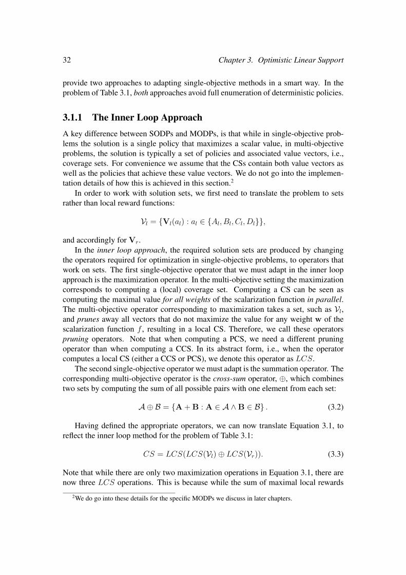
32 Chapter 3. Optimistic Linear Support
provide two approaches to adapting single-objective methods in a smart way. In theproblem of Table 3.1, both approaches avoid full enumeration of deterministic policies.
3.1.1 The Inner Loop ApproachA key difference between SODPs and MODPs, is that while in single-objective prob-lems the solution is a single policy that maximizes a scalar value, in multi-objectiveproblems, the solution is typically a set of policies and associated value vectors, i.e.,coverage sets. For convenience we assume that the CSs contain both value vectors aswell as the policies that achieve these value vectors. We do not go into the implemen-tation details of how this is achieved in this section.2
In order to work with solution sets, we first need to translate the problem to setsrather than local reward functions:
Vl = Vl(al) : al ∈ Al, Bl, Cl, Dl,
and accordingly for Vr.In the inner loop approach, the required solution sets are produced by changing
the operators required for optimization in single-objective problems, to operators thatwork on sets. The first single-objective operator that we must adapt in the inner loopapproach is the maximization operator. In the multi-objective setting the maximizationcorresponds to computing a (local) coverage set. Computing a CS can be seen ascomputing the maximal value for all weights of the scalarization function in parallel.The multi-objective operator corresponding to maximization takes a set, such as Vl,and prunes away all vectors that do not maximize the value for any weight w of thescalarization function f , resulting in a local CS. Therefore, we call these operatorspruning operators. Note that when computing a PCS, we need a different pruningoperator than when computing a CCS. In its abstract form, i.e., when the operatorcomputes a local CS (either a CCS or PCS), we denote this operator as LCS.
The second single-objective operator we must adapt is the summation operator. Thecorresponding multi-objective operator is the cross-sum operator, ⊕, which combinestwo sets by computing the sum of all possible pairs with one element from each set:
A⊕ B = A + B : A ∈ A ∧B ∈ B . (3.2)
Having defined the appropriate operators, we can now translate Equation 3.1, toreflect the inner loop method for the problem of Table 3.1:
CS = LCS(LCS(Vl)⊕ LCS(Vr)). (3.3)
Note that while there are only two maximization operations in Equation 3.1, there arenow three LCS operations. This is because while the sum of maximal local rewards
2We do go into these details for the specific MODPs we discuss in later chapters.

3.1. Inner Loop versus Outer Loop 33
in the single-objective problem form a single value when summed, the combination oftwo sets may contain combinations that are dominated.
We have now defined the general schema for creating a multi-objective inner loopmethod from a base single-objective method, i.e., replace the maximizations by prun-ing operations, and replace the summations by cross-sums. Before we can use such amethod in practice however, we must:
(a) define appropriate implementations of LCS depending on what type of solutionset we are after, e.g., a CCS or a PCS,
(b) select the places in the algorithm where pruning is applied, and
(c) check whether the resulting inner loop method is indeed correctly outputting theCS. In particular, we check that no necessary vectors for computing the CS prunedprematurely, and that no excess vectors, i.e., vectors that are never optimal for anyallowed scalarization, retained in the output.
First, let us address (a). We provide a possible implementation of LCS for thecase of CCS computations in Algorithm 1. We use this implementation throughoutthis dissertation, and refer to it as CPrune. CPrune is based on the algorithm for CCSpruning3 by Feng and Zilberstein (2004), with one modification. In order to improveruntime guarantees, CPrune first pre-prunes the input set, V , to a PCS using the PPrunealgorithm (Algorithm 2) at line 1. PPrune computes a PCS in O(d|V||PCS|) time byrunning pairwise comparisons. Next, a partial CCS, V∗, is constructed as follows: arandom vector V from V ′ is selected at line 4. For V the algorithm tries to find aweight vector w for which V is better than the vectors in V∗ (line 5), by solving thelinear program in Algorithm 3. If there is such a w, CPrune finds the best vector V′
for w in V ′ and moves it to V∗ (line 10–12). If there is no weight for which V is better,it is C-dominated and thus removed from V ′ (line 7).Theorem 2. The computational complexity of CPrune as defined by Algorithm 1 is
O(d|V||PCS|+ |PCS|P (d|CCS|)), (3.4)
where P (d|CCS|) is a polynomial in the size of the CCS and the number of objectivesd, which is the runtime of the linear program that tests for C-domination (Algorithm4).
Concerning (c), i.e., whether the algorithm outputs the correct CS, we provide asmall proof sketch for our simple MODP problem of Table 3.1. (In later chapters weprovide more formal proofs.) First, note that for each w, CPrune retains at least oneoptimal value vector, and removes all vectors that are not optimal for any w. Because
3The work by Feng and Zilberstein (2004) is from the POMDP literature. We explain the relationbetween POMDPs and multi-objective decision making in Section 3.2. Note that many algorithmsfor CCS pruning originate in other fields than POMDPs, such as graphics or geometry (e.g., Graham(1972)).

34 Chapter 3. Optimistic Linear Support
Algorithm 1: CPrune(V)
Input: A set of value vectors V1 V ′ ← PPrune(V)2 V∗ ← ∅3 while V ′ 6= ∅ do4 select random V from V ′5 w← findWeight(V,V∗); // identify a w where V improves V∗
6 if w=null then7 remove V from V ′ ; // there is no w where where V improves V∗
8 end9 else
10 V′ ← arg maxV∈V ′ w ·V ; // find best value vector for w
11 V ′ ← V ′ \ V′12 V∗ ← V∗ ∪ V′13 end14 end15 return V∗
Algorithm 2: PPrune(V)
Input: A set of value vectors V1 V∗ ← ∅2 while V 6= ∅ do3 V← the first element of V4 foreach V′ ∈ V do5 if V′ P V then6 V← V′ ; // Continue with V′ instead of V
7 end8 end9 Remove V, and all vectors P-dominated by V, from V
10 Add V to V∗11 end12 return V∗

3.1. Inner Loop versus Outer Loop 35
Algorithm 3: findWeight(V,V)
// Find a weight vector w, where the scalarized value of a new value
vector V is an improvement, i.e., w · V > maxV′∈V
w · V′, using a linear
program.
maxx,w
x
subject to w · (V −V′)− x ≥ 0,∀V′ ∈ Vd∑i=1
wi = 1
if x > 0 return w else return null
linear scalarization distributes over addition, i.e., w · (Vl(al)+Vr(ar)) = w ·Vl(al)+w ·Vr(ar), we know that no optimal values can be lost when performing CPrune onthe separate sets Vl and Vr, before taking the cross-sum. Furthermore, we know thatbecause CPrune is applied again after taking the cross-sum, no excess value vectorscan remain.
When we apply the inner loop method, i.e., Equation 3.3 where LCS = CPrune, tothe problem of Table 3.1 (and Figure 3.1(a)), we observe the following: when applyingCPrune to Vl and Vr, it removes one vector each. In other words, the local CCSsboth consist of three vectors. Therefore, the cross-sum of these CCSs consists of 9vectors, which is significantly less than the 16 we would get if we took the cross-sumbefore local pruning. However, in order to do the local pruning, we have to investeffort, which in this (small) problem amounts to as much work as computing the cross-sum. Therefore, we have to be careful when applying the inner loop approach; it isnot always worth the effort to prune everywhere we can. Selecting how much to prune— by choosing either to not prune at all, apply only PPrune, or to apply CPrune, ateach possible point in the algorithm — is a non-trivial design choice that may be veryproblem-specific. In Sections 4.3.1 and 4.3.3 for example, we analyze the differentdesign choices for an inner loop method for MO-CoGs.
Many algorithms in the literature on multi-objective decision problems, take aninner loop approach (e.g., the methods by Rollon (2008) and Wilson et al. (2015)for MO-CoGs, and Barrett and Narayanan (2008) and Moffaert and Nowe (2014) forMOMDPs). However, it is also possible to create multi-objective methods by creatinga shell around a single-objective method, rather than making major changes to thesingle-objective method itself, as we describe in the next subsection.

36 Chapter 3. Optimistic Linear Support
3.1.2 The Outer Loop ApproachIn an outer loop approach, an (approximate) coverage set is built incrementally, bysolving scalarized instances. In order to solve these scalarized instances, a subroutineappropriate for the single-objective version of the MODP at hand is required. For ex-ample, when we want to solve an MOMDP, an MDP solver is required as a subroutine.The solutions produced for scalarized instances are kept in a partial CCS.
Definition 16. A partial CCS, S, is a subset of a CCS, which is in turn a subset of allpossible value vectors (V = Vπ : π ∈ Π), i.e., S ⊆ CCS ⊆ V .
The basic structure of an outer loop method is given in Algorithm 4. It starts froman empty set (line 1), as a partial CCS. In each iteration, a scalarized instance (i.e.,an SODP resulting from scalarizing the MODP with a given f and a w) is selected(line 3), and solved using a single-objective subroutine (line 4). For each solution, i.e.,an optimal policy π∗w, of a scalarized instance, the multi-objective value vector Vw isretrieved. If Vw improves upon the partial CS, S — by improving the scalarized valuefor some (allowed) f and w — it is added to S (lines 5–8). This process continuesuntil some stop criterion is reached, e.g., when it can be proven that S is a CS or timeruns out.
Algorithm 4: OuterLoopMethod(m, SolveSO)
Input: An MODP, m, and a corresponding single-objective solver SolveSO.1 S ← ∅ ; // a partial CS2 while stop criterion not reached do3 mw ← select a w and scalarize m4 π∗w ← SolveSO(mw)5 Vw ← retrieve/compute the multi-objective value of π∗w6 if Vw improves upon S then7 S ← S ∪ Vw ; // add Vw (and associated π∗w) to S.8 end9 end
10 return S
The three main design choices when creating an outer loop method are:
(a) how to select scalarized instances to solve,
(b) which single-objective subroutine to use, and
(c) whether to compute the value vectors separately (by policy evaluation), or to adaptthe single-objective solver such that it returns both π∗w and Vw.
For example, in random sampling (RS) (which we use as a baseline in Roijers et al.(2015c)), scalarized instances are selected randomly, by sampling one allowed w (andf ) at each iteration and scalarizing the problem. The scalarized problem is then solved

3.2. The Scalarized Value Function 37
using, e.g., an out-of-the-box single-objective solver that produces an optimal policyfor mw, and the value vector, Vw retrieved by a standard policy evaluation algorithm.At each iteration, it is checked whether Vw is already in S or not — note that Vw
cannot be dominated when the single-objective solver is optimal, because it is optimalfor at least one scalarized instance by definition — and if not, added to S. Typically,this is done for a limited number of iterations, or until a fixed number Istop of iterationshas not produced a new value vector for S.
RS has two important advantages. Firstly, it quickly produces some result, and im-proves upon it iteratively, i.e., it is an anytime algorithm. This is a major advantageover many inner loop methods, as they typically need to run until completion to pro-duce any useful results. Secondly, RS is extremely easy to implement, as long as asuitable single-objective solver and policy evaluation method are available. However,RS also has a major downside: it is optimal only in the limit. Because of its random-ized nature, there is no guarantee that (within finite time) there will be no f and w leftfor which an improvement still exists.
More sophisticated linear scalarization weight sampling-based methods (Kim andde Weck, 2005; Van Moffaert et al., 2014) exist (in those articles referred to as weighted-sum methods), in which scalarizations are sampled on the basis of, e.g., the relativedistance of the value vectors V or the hyper-volume metric. However, these methodsalso do not provide runtime and optimality guarantees.
In Section 3.3, we present a novel algorithm which retains the advantages of RSand other outer loop methods, but is provably optimal when the single-objective sub-routines used are optimal, and produces bounded approximations when the subroutinesproduce upper and lower bounds, and runs in finite time. In order to do this, we makeuse of an analogy between finding the CCS for MODPs, and POMDP planning.
3.2 The Scalarized Value FunctionIn order to create outer loop methods that are provably optimal, run in finite time, andmake smart choices about which scalarized instances of the MODP to solve next, wefirst need to define the scalarized value function with respect to the linear scalariza-tion function (Definition 6). Note that focussing on linear scalarization is sufficient todiscover the CCS, even though the CCS can also be used in the context of non-linearscalarization.
When we look at the linearly scalarized value Vw of a value vector V as a functionof w, it becomes a hyperplane above the weight simplex. For example, the scalarizedvalues for the vectors in the CCS of Table 3.1 are shown in Figure 3.1b. Because thisis a 2-objective problem, the weight for objective 0, w0, is equal to 1 − w1. When weplot the scalarized value as a function of w1, each value vector becomes a line.
The maximal scalarized value function over a set of vectors, S , takes the maximumover all the vectors in that set.
Definition 17. A scalarized value function over a partial CCS, S, is a function that

38 Chapter 3. Optimistic Linear Support
takes a weight vector w as input, and returns the maximal attainable scalarized valuewith any payoff vector in S:
V ∗S (w) = maxVπ∈S
w ·Vπ.
If we take a complete CCS as S, the scalarized value function V ∗CCS(w) is the opti-mal scalarized value function. By definition, for every w the optimal scalarized valuefor the MODP is V ∗CCS(w). In Figure 3.1(b), the optimal scalarized value function isrepresented by the bold line segments. Similar to the scalarized value function, wedefine the set of maximizing value vectors and associated policies:
Definition 18. The optimal value vector set function with respect to S is a functionthat gives the value vectors that maximize the scalarized value for a given w:
VS(w) = arg maxVπ∈S
w ·Vπ,
Similarly, the optimal policy set ΠS(w), is the set of policies that constitute the valuevectors in VS(w).
Note that VS(w) and ΠS(w) are sets because for some w there can be multiple valuevectors that provide the same scalarized value.
Because V ∗S (w) is the maximum scalarized value for each w, it is the convex uppersurface of all of these lines (which represent the value vectors in S). Hence, V ∗S (w)and V ∗CCS(w) are piecewise linear and convex (PWLC) functions.
When considering partially observable Markov decision processes (POMDPs) (Cheng,1988; Kaelbling et al., 1998), the optimal value function is also a PWLC function. Inparticular, the belief vectors b in POMDPs correspond to our weight vectors w andthe α-vectors correspond to our value vectors V. POMDPs and MODPs are thus re-lated problems. This is an important observation, as many insights from the POMDPliterature can thus also be exploited in the context of computing CCSs for MODPs.However, while scalability in the number of states in a POMDP is key to the succesof a POMDP solver, the number of objectives in an MODP is typically small — thereare many MODPs with only two or three objectives. Therefore, scalability in the num-ber of objectives is typically less important than scalability in other properties of anMODP. In the next section, we build off a POMDP method that has poor scalability inthe number of POMDP states, but forms a good starting point for creating an MODPmethod.
3.3 The OLS AlgorithmIn this section, we present our main algorithmic contribution: optimistic linear support(OLS). OLS is a novel outer loop algorithm for computing the CCS for MODPs.

3.3. The OLS Algorithm 39
Like the random sampling (RS) method described in Section 3.1.2, OLS deals withmultiple objectives in the outer loop by employing a single-objective method as a sub-routine, and building the CCS incrementally. With each iteration of its outer loop,OLS thus adds at most one new vector to a partial CCS, S. To find this vector, OLSselects a single linear scalarization weight, w. The key difference with RS is that OLSselects this w intelligently. Specifically, OLS is optimistic: it selects the w that of-fers the maximal possible improvement — an upper bound on the difference betweenV ∗S (w) and the optimal scalarized value function V ∗CCS(w). After OLS identifies it,this w is passed to the inner loop. In the inner loop, OLS calls a problem specificsingle-objective solver to solve the single-objective decision problem that results fromscalarizing the MODP using the w selected by the outer loop. The policy that is opti-mal for this scalarized problem and its value vector are then added to the partial CCS.
The departure point for creating OLS is Cheng’s linear support (CLS) (Cheng,1988). CLS was originally designed as a pruning algorithm for POMDPs. Unfor-tunately, this algorithm is rarely used for POMDPs in practice, as its runtime is ex-ponential in the number of states. However, the number of states in a POMDP cor-responds to the number of objectives in an MODP, and while realistic POMDPs typi-cally have many states, many MODPs have only a handful of objectives. Therefore, forMODPs, scalability in the number of objectives is typically less important than scala-bility in other properties of the problem (such as the number of agents or the numberof states), making Cheng’s linear support an attractive starting point for developingefficient MODP algorithms.
Because OLS takes an arbitrary single-objective problem solver as input, it can beseen as a generic multi-objective method that applies to any cooperative MODP. Weshow that OLS chooses a w at each iteration such that, after a finite number of itera-tions, no further improvements to the partial CCS can be made and OLS can terminate.Furthermore, we bound the maximum scalarized error of the intermediate results, sothat they can be used as bounded approximations of the CCS. After defining the al-gorithm in this section, we show that OLS inherits any favorable properties from thesingle-objective subroutines it uses in Section 3.4. In subsequent chapters, we instanti-ate OLS by using different single-objective solvers for different instances of MODPs,and show how this leads to novel state-of-the-art algorithms for a variety of problems.
In this section, we assume that the single-objective solver used as a subroutine byOLS is exact, i.e., the scalarized instances are solved optimally. In other words, weassume that OLS has access to a function called SolveSODP that computes the bestpayoff vector for a given w. For now, we leave the implementation of SolveSODPabstract. As mentioned in Section 3.1.2, we can either use an adapted single-objectivesolver that returns the value vector, or we can use a separate policy evaluation step. InSection 3.5 we relax the assumption that SolveSODP needs to be exact.
OLS exploits the PWLC property of the scalarized value function, V ∗S (w) (Defini-tion 17). OLS incrementally builds up the CCS, by adding new value vectors that arefound at so-called corner weights, to an initially empty partial CCS, S. These cornerweights are the weights where V ∗S (w) changes slope in all directions. These must thus

40 Chapter 3. Optimistic Linear Support
0.0 0.2 0.4 0.6 0.8 1.0
1213
1415
16
w1
Vw
Δ
wc
0.0 0.2 0.4 0.6 0.8 1.0
1213
1415
16
w1
Vw
(a) (b)
0.0 0.2 0.4 0.6 0.8 1.0
1213
1415
16
w1
Vw
0.0 0.2 0.4 0.6 0.8 1.0
1213
1415
16
w1
Vw
(c) (d)
0.0 0.2 0.4 0.6 0.8 1.0
1213
1415
16
w1
Vw
0.0 0.2 0.4 0.6 0.8 1.0
1213
1415
16
w1
Vw
(e) (f)Figure 3.2: A run of OLS for the problem of Table 3.1. In each picture, V ∗S is indicatedby bold line segments, corner weights are indicated by vertical lines (gray for visited,and red for pending), and CCS is shown as dotted lines. (a) OLS finds two payoffvectors at the extrema, and a new corner weight wc = (0.4125, 0.5875) is found, withmaximal possible improvement ∆. (b) OLS finds a new vector at wc, and adds twonew corner weights to Q. (c and d) OLS finds another new vector and adds two newcorner weights to Q. (e) OLS does not find a new vector for the corner weight itselects, reducing the maximal possible improvement at that corner weight to 0. (f) Forthe remaining corner weights, no new vectors are found, ensuring S = CCS = CCS.

3.3. The OLS Algorithm 41
Algorithm 5: OLS(m, SolveSODP, ε)
Input: A MODP m, a single-objective subroutine SolveSODP, and max. allowed error ε1 S ← ∅ ; // a partial CCS
2 W ← ∅ ; // a set of visited weights
3 Q← an empty priority queue4 foreach extremum of the weight simplex we do5 Q.add(we,∞) ; // add the extrema to Q with infinite priority
6 end7 while ¬Q.isEmpty() ∧ ¬timeOut do8 w← Q.pop()9 Vπ ← SolveSODP(m,w)
10 W ←W ∪ w11 if Vπ 6∈ S then12 Wdel ← remove the corner weights made obsolete by V from Q, and store them13 Wdel ← w ∪Wdel ; // corner weights to remove
14 WVπ ← newCornerWeights(Vπ,Wdel,S)15 S ← S ∪ Vπ16 foreach w ∈WVπ do17 ∆r(w)← calculate improvement using maxValueLP(w,S,W)18 if ∆r(w) > ε then19 Q.add(w, ∆r(w))20 end21 end22 end23 end24 return S and the highest ∆r(w) left in Q
be weights where VS(w) and ΠS(w) (Definition 18) consist of multiple value vectorsand associated policies. Every corner weight is prioritized by the maximal possibleimprovement of finding a new value vector at that corner weight. When the maximalpossible improvement is 0, OLS knows that the partial CCS is complete.
As an example of this process, we show the entire run of OLS for the problem ofTable 3.1 in Figure 3.2. The (corner) weights where the algorithm has already searchedfor new payoff vectors are indicated by gray vertical lines, and the corner weights thatare still pending are indicated by red vertical lines.
OLS is shown in Algorithm 5. OLS takes as input: m, the MODP to be solved,the single-objective subroutine, SolveSODP, and ε, the maximal tolerable error in theresult.
We first describe how OLS is initialized. Then, we define corner weights formallyand describe how OLS identifies them. Finally, we describe how OLS prioritizes cornerweights and how this can also be used to bound the error when stopping OLS before itis done finding a full CCS.

42 Chapter 3. Optimistic Linear Support
Initialization
OLS starts by initializing the partial CCS, S, which contains the payoff vectors in theCCS that have been discovered so far (line 1 of Algorithm 5), as well as the set ofvisited weights W (line 2). Then, OLS adds the extrema of the weight simplex, i.e.,those points where all of the weight is on one objective, to a priority queue Q, withinfinite priority (line 5).
The First Iterations
The extrema that we added in the initialization are popped off the priority queue whenOLS enters the main loop (line 7), in which the w with the highest priority is selected(line 8). Because the extrema have infinite priority, they are guaranteed to be poppedoff the queue first. SolveSODP is called with w (line 9) to find V, the best payoffvector for that w.
In the algorithm, we assume that SolveSODP returns the best value vector for w.This can be done by adapting an out-of-the-box single-objective solver to return thisvalue vector, or by adding a separate policy evaluation step. In the latter case line 9 ofthe algorithm could instead be written as:
π ← SolveSODP(m,w)Vπ ← PolicyEval(m,π)
Throughout this dissertation, we assume that we can determine the exact value of Vπ
of the π that SolveSODP returns, i.e., the policy evaluation step is exact.To illustrate the situation after initialization, Figure 3.2a shows S after two pay-
off vectors of the 2-objective list combination problem of Table 3.1 have been foundby applying SolveSODP to the extrema of the weight simplex. This leads to S =(16.3, 11.8), (11.6, 15.1). Each of these vectors must be part of the CCS becauseit is optimal for at least one w: the one for which SolveSODP returned it as a solu-tion. The set of weightsW that OLS has tested so far, i.e., the extrema of the weightsimplex, are marked with vertical gray line segments.
Corner Weights
After having evaluated the extrema, S consists of d (the number of objectives) payoffvectors and associated joint actions. However, for many weights on the simplex, it doesnot yet contain the optimal payoff vector. Therefore, after identifying a new vector Vπ
to add to S, OLS must determine which new weight vectors to add to Q, and withwhat priority. Like Cheng’s linear support, OLS identifies the corner weights: theweights at the corners of the convex upper surface, i.e., the points where the PWLCsurface V ∗S (w) changes slope. To define the corner weights precisely, we define P ,the polyhedral subspace that is above V ∗S (w) (Bertsimas and Tsitsiklis, 1997). Forexample, in Figure 3.1b, P is displayed as the shaded area above the optimal scalarizedvalue function. The corner weights are the vertices of P, which can be defined by a setof linear inequalities:

3.3. The OLS Algorithm 43
Algorithm 6: newCornerWeights(Vπnew,Wdel,S)
Input: A new value vector, Vπnew, a set of obsolete corner weights, Wdel, and the
current partial CCS, S1 Vrel ←
⋃w∈Wdel
VS(w) ; // involved value vectors (see Definition 18)
2 Brel ← the set of boundaries of the weight simplex involved in any w ∈Wdel;3 Wnew ← ∅; // new corner weights
4 foreach subset X of d− 1 elements from Vrel ∪ Brel do5 wc ← compute weight where the vectors/boundaries in X intersect with Vπ
new ;6 if wc is inside the weight simplex then7 if wc ·Vπ
new = V ∗S (wc) then8 Wnew ←Wnew ∪wc
9 end10 end11 end12 return Wnew
Definition 19. If S is the set of known payoff vectors, we define a polyhedron
P = x ∈ <d+1 : S+x ≥ ~0,∀i, wi > 0,∑i
wi = 1,
where S+ is a matrix with the elements of S as row vectors, augmented by a columnvector of −1’s. The set of linear inequalities S+x ≥ ~0, is supplemented by the simplexconstraints: ∀i wi > 0 and
∑iwi = 1. The vector x = (w1, ..., wd, Vw) consists of
a weight vector and a scalarized value at those weights. The corner weights are theweights contained in the vertices of P , which are also of the form (w1, ..., wd, Vw).
Note that, due to the simplex constraints, P is only d-dimensional. Furthermore, theextrema of the weight simplex are special cases of corner weights.
After identifying the new value vector Vπ, OLS identifies which corner weightschange in the polyhedron P by adding Vπ to S. Fortunately, this does not require re-computation of all the corner weights, but can be done incrementally: first, the cornerweights in Q for which Vπ yields a better scalarized value than currently known aredeleted from the queue (line 12) and then the function newCornerWeights(Vπ,Wdel,S) (line 14) calculates the new corner weights that involve Vπ.
The function newCornerWeights(Vπ,Wdel, S) (Algorithm 6) first calculates theset of all relevant payoff vectors, Vrel, by taking the union of all the maximizing vec-tors of the weights in Wdel for S (on line 1). In our implementation, we optimize thisstep by caching VS(w) (Definition 18) and associated policies for all w in Q. If fora corner weight, w, VS(w) contains fewer than d value vectors, then a boundary ofthe weight simplex is involved. These boundaries are also stored (line 2). All pos-sible subsets of size d−1 — of both vectors and boundaries — are taken. For eachsubset the weight where these d − 1 payoff vectors (and boundaries) intersect with

44 Chapter 3. Optimistic Linear Support
each other and V is computed by solving a system of linear equations (on line 5). Theintersection weights for all subsets together form the set of candidate corner weights:Wcan. newCornerWeights(Vπ,Wdel, S) returns the subset of Wcan which are insidethe weight simplex and for which there is no vector V′ ∈ S that has a higher scalar-ized value than V at that weight. OLS then adds the new corner weights returned bynewCornerWeights(Vπ, Wdel,S) to its queue, Q.
In Figure 3.2a, after computing the value vectors for the two extrema, one new cor-ner weight is produced, labelled wc = (0.4125, 0.5875). In the subsequent iterationswhere a new value vector is identified (Figure 3.2b-d), two new corner weights areproduced. For two objectives, there are always (at most) two new corner weights periteration, and two value vectors involved in each corner weights. For higher numberof objectives, it is in theory possible to construct a partial CCS, S that has a cornerweight for which all payoff vectors in S are in Vrel, leading to very many new cornerweights. In practice however, |Vrel| is typically very small, and only a few systems oflinear equations need to be solved, leading to a limited number of new corner weights.
After calculating the new corner weights WVπ at line 14 (in Algorithm 5), V isadded to S at line 15. Cheng showed that finding the best payoff vector for each cornerweight and adding it to the partial CCS, guarantees the best improvement to S:
Theorem 3. (Cheng, 1988) The maximum value of:
maxw,V∈CCS
minV′∈S
w ·V −w ·V′,
i.e., the maximal improvement to S by adding a vector to it, is at one of the cornerweights.
Theorem 3 guarantees the correctness of OLS: after all corner weights are checked,there are no new payoff vectors; thus the maximal improvement must be 0 and OLShas found the full CCS (as is the case in Figure 3.2f).
Prioritization
Cheng’s linear support assumes that all corner weights can be checked inexpensively,which is a reasonable assumption in a POMDP setting. However, since SolveSODP
is typically an expensive operation, testing all corner weights may not be feasible inMODPs. For example, in MO-CoGs, a common choice for SolveSODP is the variableelimination algorithm (which we discuss in detail in the next chapter), whose runtimecan be exponential in the size of the problem. Therefore, unlike Cheng’s linear support,OLS pops only one w off Q to be tested per iteration. Making OLS efficient thuscritically depends on giving each w a suitable priority when adding it toQ. To this end,OLS prioritizes each corner weight w according to its maximal possible improvement,an upper bound on the improvement to V ∗S (w) that can be made by adding a singlenew value vector. This upper bound is computed with respect to CCS, the optimistichypothetical CCS, i.e., the best-case scenario for the final CCS given that S is the

3.3. The OLS Algorithm 45
current partial CCS and W is the set of weights already tested with SolveSODP. Akey advantage of OLS over Cheng’s linear support is thus that these priorities can becomputed without calling SolveSODP, obviating the need to run SolveSODP on allcorner weights.
Definition 20. An optimistic hypothetical CCS, CCS is a set of payoff vectors thatyields the highest possible scalarized value for all possible w consistent with findingthe vectors S at the weights inW .
In Figure 3.2a the CCS = (16.3, 11.8), (11.6, 15.1), (16.3, 15.1). CCS is a supersetof S and the value of V ∗
CCS(w) (indicated by the dotted line) is the same as V ∗S (w) at
all the weights inW . For a given w, maxValueLP(w,S,W) finds the scalarized valueof V ∗
CCS(w) by solving the following linear program (LP):
max w · vsubject to W v ≤ V∗S,W ,
where V∗S,W is a vector containing V ∗S (w′) for all w′ ∈ W , and v is a vector ofvariables of length d. Note that we abuse the notationW , which in this case is a matrixwhose rows correspond to all the weight vectors in the setW .4
Using CCS, we can define the maximal possible improvement of each w:
∆(w) = V ∗CCS
(w)− V ∗S (w).
Figure 3.2a shows ∆(wc) with a dashed line. We use the maximal relative possibleimprovement, ∆r(w) = ∆(w)/V ∗
CCS(w), as the priority of each new corner weight
w ∈ WV. In Figure 3.2a, ∆r(wc)=(0.4125,0.5875)·((16.3,15.1)−(11.6,15.1))
13.65625=0.141968. When
a corner weight w is identified (line 14), it is added to Q with priority ∆r(w) as longas ∆r(w) > ε (lines 17-19). In Figure 3.2 the corner weights in Q are indicated by redvertical line segments.
After wc in Figure 3.2a is added to Q, it is popped off again (as it is the onlyelement of Q). SolveSODP(wc) generates a new value vector (13.9, 14.3), yieldingS = (16.3, 11.8), (11.6, 15.1), (13.9, 14.3), as illustrated in Figure 3.2b. The newcorner weights are the points at which (13.9, 14.3) intersects with (16.3, 11.8) and(11.6, 15.1). Testing these weights, as illustrated in Figure 3.2cd, results in 2 new pay-off vectors, and two new corner weights each. After these two value vectors however,checking the weight with the highest priority in Q does not result in a new vector, re-ducing the maximal possible improvement at that weight to 0 (Figure 3.2e). Checkingthe remaining 3 corner weights in Q, also does not lead to new value vectors, causingOLS to terminate. Because the maximal improvement at these corner weights is 0 upontermination, S = CCS due to Theorem 3. OLS called SolveSODP for only 9 weightsresulting exactly in the 5 payoff vectors of the CCS. The other 7 payoff vectors in V(the black points of Figure 3.1) were never generated.
4 Our implementation of OLS reduces the size of the LP by using only the subset of weights inWfor which the policies involved in w, ΠS(w), have been found to be optimal. This can lead to a slightoverestimation of V ∗
CCS(w).

46 Chapter 3. Optimistic Linear Support
3.4 AnalysisWe now analyze the computational and space complexity of OLS. Because OLS is ageneric algorithm that takes a single-objective solver (and possibly a policy evaluationalgorithm) as a subroutine, we provide the complexity bounds of OLS in terms ofthe runtime and space complexities of these subroutines. We denote the runtime ofa single-objective solver as Rso and the runtime of policy evaluation as Rpe, and thecorresponding memory as Mso and Mpe.
Theorem 4. The runtime of OLS is
O( (|ε−CCS|+ |Wε−CCS|)(Rso +Rpe +Rnw +Rheur) ),
where |ε−CCS| is the size of the ε-CCS (Definition 13) outputted by OLS, |Wε−CCS| isthe number of corner weights of the scalarized V ∗ε−CCS(w) corresponding to the outputε-CCS, Rnw the time it takes to run newCornerWeights, and Rheur the time it takes tocompute the value of the optimistic CCS using maxValueLP.
Proof. The runtime of one iteration of OLS is the cost of running the single-objectivesolver plus policy evaluation, Rso + Rpe, plus the overhead per corner weight Rnw +Rheur, multiplied by the number iterations. To count the number of iterations, weconsider two cases: calls to the single-objective solver that result in adding a newvector to the partial CCS, S and those that do not result in a new vector but insteadconfirm the optimality of the scalarized value V ∗S (w) at that weight. The former is thesize of the output of OLS, i.e., |ε−CCS|, while the latter is at most the number of cornerweights of the scalarized value function of that same output set, |Wε−CCS|.
Note that we can often adapt the implementation of SolveSODP to return the valuevector of the optimal policy for a weight, alongside this optimal policy, without anincrease in the complexity bounds of the single-objective solver. In this case Rpe be-comes 0.
We have experienced that the overhead of OLS itself, i.e., computing new cornerweights, Rnw, and calculating the maximal relative improvement, Rheur, is very smallcompared to the SolveSODP for the decision problems that we study in this dissertation.In practice, newCornerWeights(u, Wdel, S) computes the solutions to only a smallset of linear equations (of d equations each). maxValueLP(w, S, W) computes thesolutions to linear programs, which is polynomial in the size of its inputs.5
If ε 6= 0, OLS does in practice not test all the corner weights of the polyhedronspanned by the ε-CCS it outputs, as OLS only tests a corner weight if the maximalpossible improvement is larger than ε. However, this cannot be guaranteed in general.Note that if ε = 0, OLS outputs an exact CCS, and needs to check every corner weightin order to establish that it is in fact an exact CCS.
5When the reduction in Footnote 4 is used, only a very small subset of W is used, making it evensmaller.
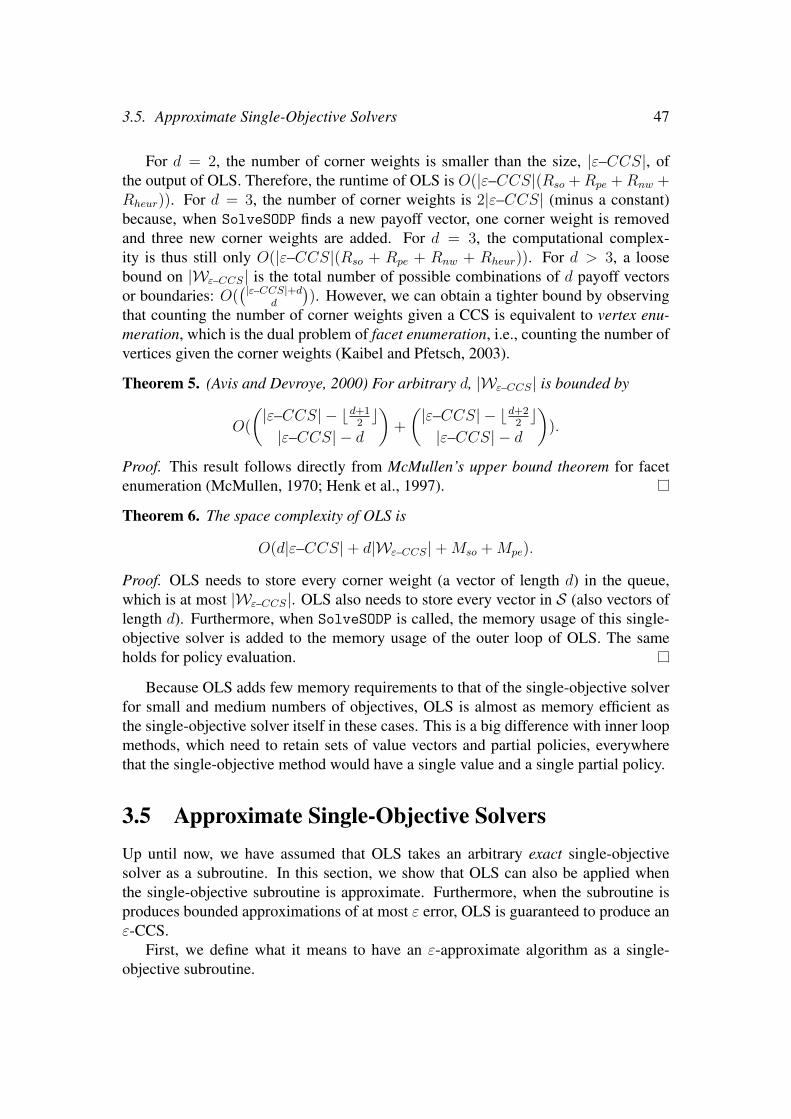
3.5. Approximate Single-Objective Solvers 47
For d = 2, the number of corner weights is smaller than the size, |ε–CCS|, ofthe output of OLS. Therefore, the runtime of OLS is O(|ε–CCS|(Rso +Rpe +Rnw +Rheur)). For d = 3, the number of corner weights is 2|ε–CCS| (minus a constant)because, when SolveSODP finds a new payoff vector, one corner weight is removedand three new corner weights are added. For d = 3, the computational complex-ity is thus still only O(|ε–CCS|(Rso + Rpe + Rnw + Rheur)). For d > 3, a loosebound on |Wε–CCS| is the total number of possible combinations of d payoff vectorsor boundaries: O(
(|ε–CCS|+dd
)). However, we can obtain a tighter bound by observing
that counting the number of corner weights given a CCS is equivalent to vertex enu-meration, which is the dual problem of facet enumeration, i.e., counting the number ofvertices given the corner weights (Kaibel and Pfetsch, 2003).
Theorem 5. (Avis and Devroye, 2000) For arbitrary d, |Wε–CCS| is bounded by
O(
(|ε–CCS| − bd+1
2c
|ε–CCS| − d
)+
(|ε–CCS| − bd+2
2c
|ε–CCS| − d
)).
Proof. This result follows directly from McMullen’s upper bound theorem for facetenumeration (McMullen, 1970; Henk et al., 1997).
Theorem 6. The space complexity of OLS is
O(d|ε–CCS|+ d|Wε–CCS|+Mso +Mpe).
Proof. OLS needs to store every corner weight (a vector of length d) in the queue,which is at most |Wε–CCS|. OLS also needs to store every vector in S (also vectors oflength d). Furthermore, when SolveSODP is called, the memory usage of this single-objective solver is added to the memory usage of the outer loop of OLS. The sameholds for policy evaluation.
Because OLS adds few memory requirements to that of the single-objective solverfor small and medium numbers of objectives, OLS is almost as memory efficient asthe single-objective solver itself in these cases. This is a big difference with inner loopmethods, which need to retain sets of value vectors and partial policies, everywherethat the single-objective method would have a single value and a single partial policy.
3.5 Approximate Single-Objective SolversUp until now, we have assumed that OLS takes an arbitrary exact single-objectivesolver as a subroutine. In this section, we show that OLS can also be applied whenthe single-objective subroutine is approximate. Furthermore, when the subroutine isproduces bounded approximations of at most ε error, OLS is guaranteed to produce anε-CCS.
First, we define what it means to have an ε-approximate algorithm as a single-objective subroutine.

48 Chapter 3. Optimistic Linear Support
Algorithm 7: AOLS(m, approxSolveSODP, ε)
Input: An MODP m, an approximate SODP subroutine ApproxSolveSODP, and max.allowed error, ε.
1 S ← ∅ ; // a partial CCS
2 W ← ∅ ; // set of tuples of visited weights and upper bounds, Vw3 Q← an empty priority queue4 foreach extremum of the weight simplex we do5 Q.add(we,∞) ; // add the extrema to Q with infinite priority
6 end7 while ¬Q.isEmpty() ∧ ¬timeOut do8 w← Q.pop()9 Vπ, Vw ← approxSolveSODP(m,w)
10 W ←W ∪ (w, Vw)11 if Vπ 6∈ S then12 Wdel ← remove the corner weights made obsolete by V from Q, and store them13 Wdel ← w ∪Wdel ; // corner weights to remove
14 WVπ ← newCornerWeights(Vπ,Wdel,S)15 remove vectors from S that are no longer optimal for any w when Vπ is added16 S ← (S ∪ Vπ)17 foreach w ∈WVπ do18 ∆r(w)← calculate improvement using maxValueLP(w,S,W)19 if ∆r(w) > ε then20 Q.add(w, ∆r(w))21 end22 end23 end24 end25 return S and the highest ∆r(w) left in Q
Definition 21. An ε-approximate SODP solver is an algorithm that produces a policywhose value is at least (1 − ε)V∗, where V ∗ is the optimal value for the SODP andε ≥ 0.
Given an ε-approximate SODP solver we can compute a set of policies for whichthe scalarized value for each possible w is at least 1 − ε times the optimal scalarizedvalue, i.e., an ε-CCS (Definition 13). To this end we change the OLS algorithm inorder to handle approximate solvers, leading to the approximate OLS (AOLS) algorithm(Algorithm 7). The differences with OLS (Algorithm 5) are highlighted in blue. Wego through the differences one by one.
Firstly, in Algorithm 7 we assume that the single-objective subroutine — in this al-gorithm referred to as approxSolveSODP — returns both the value vector and policy6,
6We assume that the value Vπ is the correct value vector of π, i.e., the evaluation of the policy valueis exact.

3.5. Approximate Single-Objective Solvers 49
Vπ, and an upper bound on the scalarized value at the weight w for which it is called,Vw (line 9). This upper bound is stored alongside w (lines 2 and 10), and used insteadof the scalarized values in maxValueLP. Specifically, for a given w, maxValueLP finds(line 18) the scalarized value of V ∗
CCS(w) by solving:
max w · vsubject to W ′ v ≤ V∗S,W ,
where for each tuple (w, Vw) ∈ W , there is a row in the matrixW ′ corresponding tow with a corresponding element Vw in the vector V∗S,W .
Secondly, because we have an approximate single-objective subroutine, the vectorsin the partial CCS S, may not be optimal for any w anymore when we add a new valuevector. Therefore, we first have to remove these vectors from S (line 15). We cando this efficiently, by checking whether Vπ is better than a vector V′ ∈ S for all thecorner weights of V ∗S (w) for which V′ is optimal, as this bounds the area for which V′
is optimal w.r.t. to the other value vectors currently in S.
Correctness
We now establish the correctness of Algorithm 7, i.e., OLS with approximate single-objective subroutines. Because the scalarized value of V ∗
CCS(w) (as computed by
maxValueLP) obtained through using the ε of the approximate solveMDP is no longeridentical to V ∗S (w), we need to make an adjustment to Cheng’s theorem.
Theorem 7. There is a corner weight of V ∗S (w) that maximizes:
∆(w) = V ∗CCS(w)− V ∗S (w),
where S is an intermediate set of value vectors computed by AOLS (Algorithm 7).
This theorem is identical to Cheng’s, but, because S is no longer a subset of the CCS,the proof is different.
Proof. ∆(w) is the difference between two PWLC functions: V ∗CCS(w) and V ∗S (w).To maximize this function, we have three possible cases, shown in Figure 3.3: (a) themaximum is at a weight that is neither a corner point of V ∗CCS(w), nor of V ∗S (w); (b)it is at a corner point of V ∗CCS(w) but not of V ∗S (w); or (c) it is at a corner point ofV ∗S (w).
Case (a) can only apply if the slope of ∆(w) at w is 0, if this is so, then thevalue of ∆(w) is equal to the value at the corner points where this slope changes.Case (b) can never occur: if w is a corner point of V ∗CCS(w), and not of V ∗S (w), and∆(w) = V ∗CCS(w) − V ∗S (w) is at a maximum, then because V ∗S (w) does not changeslope in w, the change in slope for V ∗CCS(w) must be negative. However, because weknow that V ∗CCS(w) is a PWLC function, this leads to a contradiction. Therefore, onlycase (c) remains.

50 Chapter 3. Optimistic Linear Support
(a) (b) (c)Figure 3.3: Possible cases for the maximum possible improvement of S with respectto the CCS.
Because the maximum possible improvement is still at the corner points of S,even though S now contains ε-approximate solutions, the original scheme of calling asingle-objective subroutine for the corner weights still applies.
The approximate-subroutine version of OLS terminates when the maximal possibleimprovement is less than or equal to ε · V ∗
CCS(w). In other words, when there are no
corner weights with a possible improvement higher than the input slack ε.
Theorem 8. AOLS — as specified in Algorithm 7 — terminates after a finite number ofcalls to an ε-approximate SODP solver approxSolveSODP and produces an ε-CCS.
Proof. The algorithm runs until there are no corner points left in the priority queue tocheck, and returns S and the highest priority left inQ. Once a corner point is evaluated,it is never considered again because the established value lies within (1− ε)V ∗
CCS(w)
(as guaranteed by the ε-bound of approxSolveSODP). AOLS thus terminates afterchecking a finite number of corner weights. All other corner weights have a possibleimprovement less than or equal to εV ∗
CCS(w). Therefore S must be an ε-CCS.
An equivalent, but subtly different version of the approximate OLS algorithm andthe corresponding correctness theorem, can be established accordingly, when the single-objective subroutine provides an upper and lower bound (implying an ε), but it cannotbe know beforehand how strict these bounds will be:
Corollary 2. When an approximate single-objective solver produces a bounded ap-proximate solution for each scalarized problem, with an error bound of at most ε,AOLS produces an ε-CCS.
Proof. The proof is the same as for 8, by assuming that there is some ε for whichapproxSolveSODP is ε-approximate, and establishing this on the fly, by inspecting thedifference between the upper and lower bounds found by the ε-approximate solver.
Note that the runtime and memory requirements, as established in Theorems 4 and6, are not affected by the usage of an approximate single-objective subroutine insteadof an exact one, in any way other than changing the value of Rso, and Mso.

3.6. Value reuse 51
3.6 Value reuse
Figure 3.4: Close cornerweights lead to close valuevectors.
One possible issue with using OLS in practice is thatfor every corner weight w, the single-objective sub-routine is called. When there are many corner weights,this may take a long time, especially when the single-objective solver need to start from scratch. However,in many cases, we might be able to reuse part of thework done in earlier iterations of OLS, in order to hot-start the single-objective subroutine for a new w.
The key insight behind reuse in OLS, is that whentwo corner weights, w and w′, are similar, the valuevectors for these weights found by the single-objectivesolver are also likely to be similar, (e.g., in Figure 3.4).Therefore, we also expect that similar policies are op-timal for w′. If that is indeed the case, and we have a single-objective subroutine thatcan start from a previous solution — or part of this previous solution — and graduallyimprove, this may save us a lot of runtime.
In Algorithm 8, we show how this could be implemented. The differences with Al-gorithm 7 are shown in blue. We aim to show the most general form of the algorithm,and therefore use an abstract data type Iw that represents any possible informationfrom a previous call to approxSolveSODP for a weight w, that we may reuse in sub-sequent iterations. Which information can be reused depends on the specifics of theMODP, e.g., the full state-value function of a MO(PO)MDP (Chapter 5), or a repa-rameterization used by variational methods for coordination graphs (Chapter 4). Weassume that this information is produced by the single-objective solver (line 10), andis stored together with the previous search weights (lines 2 and 11). At every iteration,all possibly reusable information from all previous iterations, I , is retrieved (line 9)and used to hot-start the single-objective subroutine on line 10.
Without further assumptions, reuse is a heuristic, i.e., it may improve the runtime inpractice, but it does not show up in the complexity results for the algorithm. However,if we can assume that I contains enough information for approxSolveSODP to checkthat S is already sufficient for the new weight w, and that this check can be performedin Rconfirm, we do not require a full run of the single-objective subroutine for cornerweights for which we will not find a new value vector, and can reduce the theoreticalruntime guarantees.
Theorem 9. The runtime of OLS with reuse is
O( (|ε−CCS|)(Rso +Rpe +Rnw +Rheur) + |Wε−CCS|Rconfirm ),
where Rconfirm is the time it takes to check the sufficiency of the solutions currently inW and their value vectors S.

52 Chapter 3. Optimistic Linear Support
Algorithm 8: OLS+R(m, approxSolveSODP, ε)
Input: An MODP m, an approximate SODP subroutine ApproxSolveSODP, and max.allowed error, ε.
1 S ← ∅ ; // a partial CCS
2 W ← ∅ ; // a set of tuples of w, Vw and Iw3 Q← an empty priority queue;4 foreach extremum of the weight simplex we do5 Q.add(we,∞) ; // add the extrema to Q with infinite priority
6 end7 while ¬Q.isEmpty() ∧ ¬timeOut do8 w← Q.pop();9 I ← Retrieve the reusable information for relevant previous iterations fromW;
10 Vπ, Vw, Iw ← approxSolveSODP(m,w, I) ;11 W ←W ∪ (w, Vw, Iw);12 if Vπ 6∈ S then13 Wdel ← remove the corner weights made obsolete by V from Q, and store them14 Wdel ← w ∪Wdel ; // corner weights to remove
15 WVπ ← newCornerWeights(Vπ,Wdel,S);16 remove vectors from S that are no longer optimal for any w when Vπ is added;17 S ← (S ∪ Vπ);18 foreach w ∈WVπ do19 ∆r(w)← calculate improvement using maxValueLP(w,S,W);20 if ∆r(w) > ε then21 Q.add(w, ∆r(w));22 end23 end24 end25 end26 return S and the highest ∆r(w) left in Q
This is especially important when the number of objectives is high, because — aswe have seen in Theorem 5 — |Wε−CCS| increases exponentially with the number ofobjectives. Note however, that the greater the amount of information stored per w, themore memory per corner weight OLS with reuse uses. We discuss problem-specificinstances of this algorithm, implementing reuse for the various problems we discuss inthis dissertation in the following chapters.

Chapter 4Coordination
In cooperative multi-agent settings agents must coordinate their behavior in order tooptimize their common team payoff. Key to making coordination between agents ef-ficient is exploiting the loose couplings common to such tasks: each agent’s actionsdirectly affect only a subset of the other agents. Multi-objective coordination graphs(MO-CoGs) (Definition 27) express such independence in a graphical model for single-shot decisions. In this chapter, we propose new methods for MO-CoGs that computethe convex coverage set (CCS).
The single-objective version of MO-CoGs, i.e., coordination graphs (CoGs), iswell-studied, and many methods to exploit loose couplings exist, including variableelimination (Rosenthal, 1977; Dechter, 1998; Guestrin et al., 2002; Kok and Vlassis,2006), AND/OR tree search (Dechter and Mateescu, 2007; Marinescu, 2008; Mateescuand Dechter, 2005; Yeoh et al., 2010), and variational methods (Wainwright and Jor-dan, 2008; Liu and Ihler, 2011; Sontag et al., 2011; Ihler et al., 2012). For MO-CoGs,several methods (Delle Fave et al., 2011; Dubus et al., 2009a; Marinescu et al., 2012)that have previously been developed build upon a single-objective method using an in-ner loop approach. These methods typically compute a Pareto coverage set (PCS). Forinstance, Rollon (2008) introduces an inner-loop algorithm that we refer to as multi-objective variable elimination (MOVE), which builds upon the variable eliminationalgorithm and solves multi-objective coordination graphs by iteratively solving localproblems to eliminate agents from the graph. In this dissertation (i.e., Section 2.3)however, we argue that the PCS is often not the most appropriate solution concept.Therefore, we propose novel algorithms that compute the CCS rather than the PCS.We define both inner and outer loop methods, and compare them to each other.
Before we can propose multi-objective methods however, we must first providebackground on the single-objective methods upon which these methods build, as wellas single-objective coordination graphs, in Section 4.1. Then, in Section 4.2, we definemulti-objective coordination graphs formally.
In Section 4.3 we propose novel inner loop methods that compute a CCS for MO-CoGs. We propose convex multi-objective variable elimination (CMOVE) in Section
53

54 Chapter 4. Coordination
4.3.1, that builds upon variable elimination, and convex tree-search (CTS) in Section4.3.3 that builds upon AND/OR tree search. Both CMOVE and CTS are exact methods,but while CMOVE is fast and uses a lot of memory, CTS focusses on situations inwhich limited memory is available.
In Section 4.4, we propose our novel outer loop methods. Firstly, we proposevariable elimination linear support (VELS) that combines our outer loop approach —OLS (Chapter 3) — with variable elimination, and tree search linear support (TSLS)that combines AND/OR tree search with OLS. Because VELS and TSLS are basedon the same single-objective methods as CMOVE respectively CTS, comparing thesemethods provides a fair comparison between outer and inner loop methods.
Finally, we introduce variational optimistic linear support (VOLS) that combinesOLS with variational methods. For VOLS, it is not clear how to create a correspond-ing inner loop method, as variational methods do not have explicit maximization andsummation as their core operators. However, VOLS is an important addition to theaforementioned outer loop methods; it is not exact — though it provides a bounded ap-proximation — but makes up for this lack of optimality with very favorable empiricalruntime results.
The results of comparing our algorithms to PCS methods indicate that computingthe CCS is typically much less computationally intensive than computing a PCS. Fur-thermore, the results indicate that the outer loop approach is typically much faster thanthe inner loop approach for small and medium numbers of objectives. We concludewith a summary of the available trade-offs that our novel algorithms pose with respectto runtime, memory-usage, and quality of the output set in Section 4.5.
4.1 Coordination Graphs
Before going into MO-CoGs, we first provide background on the corresponding single-objective problem, i.e., coordination graphs (CoGs) (Guestrin et al., 2002; Kok andVlassis, 2004), and methods for solving them. Our — and several existing — methodsfor solving MO-CoGs build upon these single-objective methods.
In the context of coordination graphs, what we called reward for bandits is typicallycalled payoff in the literature. Payoff is usually denoted u (for utility). We adopt thisterminology in this dissertation when talking about coordination graphs.
Definition 22. A coordination graph (CoG) (Guestrin et al., 2002; Kok and Vlassis,2004) is a tuple 〈D,A,U〉, where
• D = 1, ..., n is the set of n agents,
• A = Ai × ... × An is the joint action space: the Cartesian product of the finiteaction spaces of all agents. A joint action is thus a tuple containing an actionfor each agent a = 〈a1, ..., an〉, and
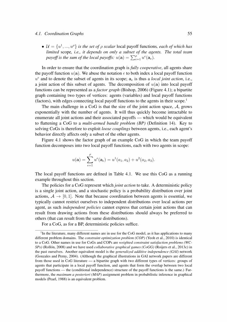
4.1. Coordination Graphs 55
• U = u1, ..., uρ is the set of ρ scalar local payoff functions, each of which haslimited scope, i.e., it depends on only a subset of the agents. The total teampayoff is the sum of the local payoffs: u(a) =
∑ρe=1 u
e(ae).
In order to ensure that the coordination graph is fully cooperative, all agents sharethe payoff function u(a). We abuse the notation e to both index a local payoff functionue and to denote the subset of agents in its scope; ae is thus a local joint action, i.e.,a joint action of this subset of agents. The decomposition of u(a) into local payofffunctions can be represented as a factor graph (Bishop, 2006) (Figure 4.1); a bipartitegraph containing two types of vertices: agents (variables) and local payoff functions(factors), with edges connecting local payoff functions to the agents in their scope.1
The main challenge in a CoG is that the size of the joint action space, A, growsexponentially with the number of agents. It will thus quickly become intractable toenumerate all joint actions and their associated payoffs — which would be equivalentto flattening a CoG to a multi-armed bandit problem (BP) (Definition 14). Key tosolving CoGs is therefore to exploit loose couplings between agents, i.e., each agent’sbehavior directly affects only a subset of the other agents.
Figure 4.1 shows the factor graph of an example CoG in which the team payofffunction decomposes into two local payoff functions, each with two agents in scope:
u(a) =
ρ∑e=1
ue(ae) = u1(a1, a2) + u2(a2, a3).
The local payoff functions are defined in Table 4.1. We use this CoG as a runningexample throughout this section.
The policies for a CoG represent which joint action to take. A deterministic policyis a single joint action, and a stochastic policy is a probability distribution over jointactions, A → [0, 1]. Note that because coordination between agents is essential, wetypically cannot restrict ourselves to independent distributions over local actions peragent, as such independent policies cannot express that certain joint actions that canresult from drawing actions from these distributions should always be preferred toothers (that can result from the same distributions).
For a CoG, as for a BP, deterministic policies suffice.
1In the literature, many different names are in use for the CoG model, as it has applications to manydifferent problem domains. The constraint optimization problem (COP) (Yeoh et al., 2010) is identicalto a CoG. Other names in use for CoGs and COPs are weighted constraint satisfaction problems (WC-SPs) (Rollon, 2008) and we have used collaborative graphical games (CoGG) (Roijers et al., 2013c) inthe past ourselves. Another equivalent model is the generalized additive independence (GAI) network(Gonzales and Perny, 2004). (Although the graphical illustrations in GAI network papers are differentfrom those used in CoG literature — a bipartite graph with two different types of vertices: groups ofagents that participate in a local payoff function, and agents that form the overlap between two localpayoff functions — the (conditional independence) structure of the payoff functions is the same.) Fur-thermore, the maximum a posteriori (MAP) assignment problem in probabilistic inference in graphicalmodels (Pearl, 1988) is an equivalent problem.

56 Chapter 4. Coordination
3 1 2 3
u u 1 2
Figure 4.1: A CoG with 3 agents and 2 local payoff functions. The factor graph illustrates theloose couplings that result from the decomposition into local payoff functions. In particular,each agent’s choice of action directly depends only on those of its immediate neighbors, e.g.,once agent 1 knows agent 2’s action, it can choose its own action without considering agent 3.
a2 a2
a1 3.25 0
a1 1.25 3.75
a3 a3
a2 2.5 1.5
a2 0 1
Table 4.1: The payoff matrices for u1(a1, a2) (left) and u2(a2, a3) (right). There aretwo possible actions per agent, denoted by a dot (a1) and a bar (a1).
Theorem 10. For a CoG, there is always a deterministic policy that maximizes thevalue.
Proof. We can a flatten CoG to a (very large) BP (Definition 14), i.e., we can see theteam of cooperative agents as a single centralized agent with a very large action space(i.e., A), with associated payoffs u(a), and we know that for a BP there is always adeterministic policy that maximizes the value.
Even though we can in theory flatten a CoG to a BP, this is typically not possible inpractice as the size of the action space is exponential in the number of agents, and there-fore becomes too large to enumerate for all but small numbers of agents. Therefore weneed special solution methods that exploit the structure of the reward function.Thereare many algorithms that do this; these can roughly be subdivided into four majorclasses of algorithms: message passing (Bishop, 2006; Kok and Vlassis, 2006; Vlassiset al., 2004), variable elimination (also called non-serial dynamic programming andbucket elimination) (Dechter, 1998; Rosenthal, 1977), search-based methods (Dechterand Mateescu, 2007; Furcy and Koenig, 2005; Marinescu, 2008), and variational meth-ods (Liu and Ihler, 2013; Sontag et al., 2011).
In the following subsections, we summarize the three methods that we use as astarting point to create new methods for MO-CoGs, and on which several existingmulti-objective algorithms are already based. Because message-passing algorithms

4.1. Coordination Graphs 57
typically do not have quality guarantees on the joint actions they produce; we focuson the variable elimination algorithm, which is fast and produces optimal joint ac-tions; one subclass of search-based algorithms called AND/OR tree search, which canproduce the optimal joint actions with limited memory-usage (Mateescu and Dechter,2005); and variational methods, which are fast, but do not always produce optimal jointactions. However, variational methods typically do return a bound on how much valueis lost when they do not produce the optimal joint action. Therefore, we can use thesemethods as a basis for creating multi-objective methods that produce ε-CSs.
4.1.1 Variable EliminationWe first discuss the variable elimination (VE) algorithm, on which several multi-objective extensions (e.g., Rollon and Larrosa (2006); Rollon (2008)) build, includingour own CMOVE (Section 4.3.1) and VELS (Section 4.4.1) algorithms.
VE exploits the loose couplings expressed by the local payoff functions to effi-ciently compute the optimal joint action. The optimal joint action is that joint action,a, that maximizes the team payoff, u(a). First, in the forward pass, VE eliminateseach of the agents in turn by computing the value of that agent’s best response to ev-ery possible joint action of its neighbors. These best responses are used to constructa new local payoff function that encodes the values of the best responses. The newlocal payoff function then replaces the agent and the payoff functions in which it par-ticipated. In the original algorithm, once all agents are eliminated, a backward passassembles the optimal joint action using the constructed payoff functions. Here, wepresent a slight variant in which each payoff is ‘tagged’ with the action that generatesit, obviating the need for a backwards pass. While the two algorithms are equivalent,this variant is more amenable to the multi-objective (inner loop) extension we presentin Section 4.3.1.
VE eliminates agents from the graph in a predetermined order. This order is typ-ically determined heuristically (e.g., following Koller and Friedman (2009)), becausefinding the optimal elimination order is itself NP-hard (Arnborg, 1985; Dechter, 1998).
Algorithm 9 shows pseudocode for the elimination of a single agent i. First, VEdetermines the set, Ui, of local payoff functions connected to i, and the set, ni, ofneighboring agents of i (lines 1-2).
Definition 23. The set, Ui, of neighboring local payoff functions of i is the set of alllocal payoff functions that have agent i in scope.
Definition 24. The set, ni, of neighboring agents of i is the set of all agents that are inscope of one or more of the local payoff functions in Ui.
Then, VE constructs a new local payoff function, unew(ani), by computing thevalue of agent i’s best response to each possible joint action ani of the agents in ni(lines 3-12). To do so, it loops over all these joint actions Ani (line 4). For each ani , itloops over all the actionsAi available to agent i (line 6). For each ai ∈ Ai, it computes

58 Chapter 4. Coordination
3 1 2 3
u u 1 2
1 2 1
4
a b c
u
u
3 1 u
Figure 4.2: (a) A CoG with 3 agents and 2 local payoff functions (b) after eliminating agent 3by adding u3 (c) after eliminating agent 2 by adding u4.
the local payoff when agent i responds to ani with ai (line 7). VE tags the total payoffwith ai, the action that generates it (line 8) in order to be able to retrieve the optimaljoint action later. If there are already tags present, VE appends ai to these tags. In thismanner, the entire joint action is constructed incrementally. VE maintains the value ofthe best response by taking the maximum of these payoffs, and storing this maximalpayoff in the new local payoff function, unew(ani), on line 11. After the value for eachani is computed, VE eliminates the agent and all payoff functions in Ui and replacesthem with the newly constructed local payoff function (line 13).
Algorithm 9: elimVE(U , i)Input: A set, U , of local payoff functions, and an agent i
1 Ui← set of local payoff functions involving i2 ni← set of neighboring agents of i3 unew ← a new factor taking joint actions of ni, ani , as input4 foreach ani ∈ Ani do5 S ← ∅ ; // set of action values for i6 foreach ai ∈ Ai do7 v ←
∑uj∈Ui
uj(ani , ai)
8 tag v with ai9 S ← S ∪ v
10 end11 unew(ani)← max(S); // pick maximal value
12 end13 return (U \ Ui) ∪ unew
Now, let us consider the example of Figure 4.1 and Table 4.1. The optimal payoffmaximizes the sum of the two payoff functions:
maxa
u(a) = maxa1,a2,a3
u1(a1, a2) + u2(a2, a3).

4.1. Coordination Graphs 59
The working of VE is illustrated in Figure 4.2, for the elimination order [3, 2, 1]. VEeliminates agent 3 first, by pushing the maximization over a3 inward such that goesonly over the local payoff functions involving agent 3, in this case just u2:
maxa
u(a) = maxa1,a2
(u1(a1, a2) + max
a3u2(a2, a3)
).
VE solves the inner maximization and replaces it with a new local payoff function u3
that depends only on agent 3’s neighbors, thereby eliminating agent 3:
maxa
u(a) = maxa1,a2
(u1(a1, a2) + u3(a2)
),
which leads to the new factor graph depicted in Figure 4.1b. The values of u3(a2) areu3(a2) = 2.5, using a3, and u3(a2) = 1 using a3, as these are the optimal payoffs forthe actions of agent 2, given the payoffs shown in Table 4.1.
Because we ultimately want the optimal joint action as well as the optimal payoff,VE needs to store the actions of agent 3 that correspond to the values in the new localpayoff factor. In our adaption of VE, the algorithm tags each payoff of u3 with theaction of agent 3 that generates it. We can thus think of u3(a2) as a tuple of value andtags, where value is a scalar payoff, and tags is a list of individual agent actions. Wedenote such a tuple with parentheses and a subscript: u3(a2) = (2.5)a3 , and u3(a2) =(1)a3 .
VE next eliminates agent 2, yielding the factor graph shown in Figure 4.1c:
maxa
u(a) = maxa1
(maxa2
u1(a1, a2) + u3(a2)
)= max
a1u4(a1).
VE appends the new tags for agent 2 to the existing tags for agent 3, yielding: u4(a1) =maxa2 u
1(a1, a2)+u3(a2) =(3.25)a2 +(2.5)a2a3 = (5.75)a2a3 and u4(a1) = (3.75)a2 +(1)a2a3 = (4.75)a2a3 . Finally, maximizing over a1 yields the optimal payoff — (5.75)a1a2a3— with the optimal action contained in the tags.
The computational complexity of VE is exponential in the induced width, w,
Theorem 11. (Guestrin et al., 2002) The computational complexity of VE isO(n|Amax|w)where |Amax| is the maximal number of actions for a single agent and w is the inducedwidth, i.e., the maximal number of neighboring agents of an agent plus one (the agentitself), at the moment when it is eliminated.
The induced width is limited by the number of agents; when the factor graph isfully connected, i.e., every agent shares a local payoff function with every other agent,w is equal to n. In practice however, w is typically much smaller than n.
The space complexity of VE is also exponential in the induced width:
Theorem 12. (Dechter, 1998) The space complexity of VE is O( n |Amax|w).

60 Chapter 4. Coordination
2
1 3
a b
1 3
2
ȧ ā
1 3
ȧ ā ȧ ā ȧ ā ȧ ā
2 2
1 1 3 3 1 1 3 3
Figure 4.3: (a) a pseudo tree, (b) a corresponding AND/OR search tree.
This space complexity arises because, for every agent elimination, a new localpayoff function is created with O(|Amax|w) fields (possible input actions). Since it isimpossible to tell a priori how many of these new local payoff functions exist at anygiven time during the execution of VE, this need to be multiplied by the total numberof new local payoff functions created during a VE execution, which is n.
While VE is designed to minimize runtime2 other methods focus on memory ef-ficiency instead (Mateescu and Dechter, 2005). We discuss a class of more memoryefficient — but still exact — methods in the next section.
4.1.2 AND/OR tree search
AND/OR tree search (Dechter and Mateescu, 2007; Marinescu, 2008; Mateescu andDechter, 2005; Yeoh et al., 2010) is a class of algorithms for solving CoGs that can betuned to provide better space complexity guarantees than VE. However, this improve-ment in space complexity does come at the price of a worse runtime complexity (Ma-teescu and Dechter, 2005). In this section we provide a brief background on AND/ORtree search. For a broader overview of AND/OR tree search for CoGs and related mod-els please see the work of Dechter (2013) and Marinescu (2008). For multi-objectiveversions of AND/OR tree search that compute a PCS, please see the work of Marinescu(2009, 2011).
The first step in an AND/OR tree search algorithm, is to convert the CoG to apseudo tree (PT). Given a PT, each agent need only know which actions its ancestorsand descendants in the PT take in order to select its own action. For example, if anagent i (a node) in the PT has two subtrees (T1 and T2) under it, all the agents in T1 areconditionally independent of all the agents in T2 given i and the ancestors of i. Figure4.3a shows the PT for the example CoG of Figure 4.1 and Table 4.1.
2In fact, VE is proven to have the best runtime guarantees within a large class of algorithms (Rosen-thal, 1977).

4.1. Coordination Graphs 61
Next, AND/OR tree search algorithms perform a tree search that results in anAND/OR search tree (AOST). Each agent i in an AOST is an OR-node. Its childrenare AND-nodes, each corresponding to one of agent i’s possible actions, ai ∈ Ai. Inturn, the children of these AND-nodes are OR-nodes corresponding to agent i’s chil-dren in the PT. Because each action (AND-node) of agent i has the same agents underit as OR-nodes, the agents and actions can appear in the tree multiple times. Figure4.3b shows an AOST corresponding to the PT of Figure 4.3a.
A specific joint action can be constructed by traversing the tree, starting at the rootand selecting one alternative from the children of each OR-node, i.e., one action foreach agent, and continuing down all children of each AND-node. For example, inFigure 4.3b, the joint action < a1, a2, a3 > is indicated in grey.
To retrieve the value of a joint action, we must first define the value of AND-nodes.
Definition 25. The value of an AND-node, vai , that represents an action ai of an agenti is the sum of the local payoff functions, ue(ae), that have i in scope (i.e., i ∈ e) forwhich ai, together with its AND-node ancestors’ actions, specifies a complete localjoint action, ae.
For example, in the AOST of Figure 4.3b, the total payoff of the CoG is u(a1, a2, a3)= u1(a1, a2) + u2(a2, a3). The value of the grey AND-node a3 is u2(a2, a3), as u3 isthe only payoff function that has agent 3 in scope and, together with its ancestral AND-node, the grey a2-node, a3 completes a joint local action for u2.
To retrieve the optimal action, we must define the value of a subtree in the AOST:
Definition 26. The value of a subtree v(Ti) rooted by an OR-node i in an AOST is themaximum of the value of the subtrees rooted by the (AND-node) children of i. Thevalue of a subtree v(Tai) rooted by an AND-node ai in an AOST is the value of aiitself (Definition 25) plus the sum of the value of the subtrees rooted by the (OR-node)children of ai.
The most memory-efficient way to retrieve the optimal joint action using an AOSTis performing a depth-first search and computing the values of the subtrees. By gen-erating nodes on the fly and deleting them after they are evaluated, memory usage isminimized. We refer to this algorithm simply as AND/OR tree search (TS). As in ourimplementation of VE, our implementation of TS employs a tagging scheme, taggingthe value of a subtree with the actions that maximize it.
TS has much better space complexity than VE, i.e., only linear in the number ofagents n, but a worse computational complexity:
Theorem 13. (Mateescu and Dechter, 2005) The space complexity of TS is O(n),where n is the number of agents.
Proof. Because TS performs depth-first search, creating and deleting nodes on the fly,at most O(n) nodes need to exist at any point during execution of TS.

62 Chapter 4. Coordination
Theorem 14. (Mateescu and Dechter, 2005) The computational complexity of TS isO(n|Amax|m), where n is the number of agents, |Amax| is the maximal number ofactions of a single agent and m is the depth of the pseudo tree, and uses linear space,O(n).
Proof. The number of nodes in an AOST is bounded byO(n|Amax|m). The tree createsmaximally |Amax| children at each OR-node. If every AND-node had exactly onechild, the number of nodes would be bounded by O(|Amax|m), as the PT is m deep.However, if there is branching in the PT, an AND-node can have multiple children.Each branch increases the size of the AOST by at most O(|Amax|m) nodes. Becausethere are exactly n agents in the PT, this can happen at most n times. At each node inthe AOST, TS performs either a summation of scalars, or a maximization over scalars.
The PT-depthm is a different constant than the induced widthw, and is typically larger.However, m can be bounded in w.
Theorem 15. (Dechter and Mateescu, 2007) Given a (MO-)CoG with induced widthw, there exists a pseudo tree for which the depth m ≤ w log n.
Note that this theorem hold for CoGs and MO-CoGs alike, because it concerns onlythe structure of the graphs.
To obtain PTs in practice, we perform two steps: first, we use the same heuristicas for VE to generate an elimination order and then transform it into a PT for whichm ≤ w log n holds — whose existence is guaranteed by Theorem 15 — using theprocedure proposed by Bayardo and Miranker.
Thus, combining Theorems 13, 14 and 15 shows that, when there are few agents,TS can be much more memory efficient than VE with a relatively small negative effecton the runtime.
4.1.3 Variational methodsThe CoG solvers that we have described in the previous two subsections — VE andTS — are both exact methods and their computational complexity is exponential ininduced width, or worse. In this section, we describe a class of algorithms calledvariational algorithms. Variational algorithms are not exact, but can provide a boundedapproximate solution. In return for the loss of optimality, variational methods haveruntimes that are sub-exponential in practice.
Variational algorithms (Sontag et al., 2011; Wainwright and Jordan, 2008) boundthe maximal payoff of a single-objective coordination graph. We denote this upperbound as u. At each iteration of a variational algorithm, this upper bound is tightened,by reparameterizing and possibly restructuring the CoG.
As an example of how upper bounds are computed, we use dual decomposition,which is a popular and illustrative variational algorithm.

4.1. Coordination Graphs 63
Dual decomposition relaxes the full maximization into an easily evaluated boundbased on local payoff functions, ue ∈ U ,
maxa
u(a) = maxa
∑ue∈U
ue(ae) ≤∑ue∈U
maxae
ue(ae) = u. (4.1)
Then, this bound is iteratively tightened by re-parameterizing the individual functionsin U , i.e., one finds a set of equivalent local payoffs U ′ such that the total payoff isunchanged,
∀a u′(a) =∑u′e∈U ′
u′e(ae) =∑ue∈U
ue(ae) = u(a),
while minimizing the decomposed upper bound (the right-hand side of Equation 4.1).Dual decomposition achieves the equality of u′(a) and u(ae), and the tightening of theupper bound via Lagrangian multipliers. For each original local payoff function ue(ae)with more than 1 agent in scope, dual decomposition creates a reparameterized localpayoff function u′e ∈ U ′ that is identically scoped, and is structured as:
u′e(ae) = ue(ae)−∑i∈e
λei (ai),
where, λei (ai) is the Lagrangian multiplier for agent i for the local payoff functionwith scope e, and for each agent separately, dual decomposition creates a local payofffunction, u′i(ai) ∈ U ′:
u′i(ai) = ui(ai) +∑e3i
λei (ai),
where ui(ai) represents an original payoff function with only agent i in scope (if thereis no such local payoff function in U , we assume ui(ai) = 0), and
∑e3i λ
ei (ai) is a
sum over the Lagrangian multipliers used in the larger local payoff functions u′e(ae)in which agent i participates. This ensures that the sum over all payoff functions inU ′ is identical to the sum over all payoff functions in U for all joint actions a, as theλei (ai) components of the functions with one agent and those with more than one agentin scope cancel each other out.
After it is ensured that the total team payoff stays the same for a variational method,the remaining problem of finding equivalent sets of local payoffs U ′ while minimizingthe upper bound, is a convex optimization problem and can be solved iteratively usinggradient-based or fixed-point techniques (Sontag et al., 2011).
The upper bound corresponds to an optimization of the individual ue(ae). If the op-timal local actions for each individual local payoff function a∗e are all consistent withsome global joint action a∗, then a∗ is also the global optimum of u(a). In practicehowever, the decomposition bound may not be able to find the global optimum. There-fore, variational methods typically also assemble a joint action al that provides a lowerbound
u = u(al).

64 Chapter 4. Coordination
Assembling al can for example be done by greedy assignment: for each local payoffu′e(ae), we assign the elements of ae that are not already assigned in al by maximizingthe local function, conditioned on the already-assigned elements.
4.2 Multi-objective Coordination GraphsWhen we extend the CoG to the multi-objective setting, it becomes harder to solve. Wehave to not only consider stochastic policies, but a priori scalarization of the problemcan become infeasible, even when we know the exact scalarization function, f , and itsparameters w.
Definition 27. A multi-objective coordination graph (MO-CoG) is a tuple 〈D,A,U〉in which D and A are as in a CoG but,
• U = u1, ...,uρ is a set of ρ, d-dimensional local reward functions.
The total team payoff is the sum of local vector-valued rewards: u(a) =∑ρ
e=1 ue(ae).
We use ui to indicate the value of the i-th objective.
Firstly, we observe that even when we know f , and its parameters w, but f is non-linear, it is not possible to scalarize the MO-CoG a priori while retaining the samestructure for the reward function. This is because f does not distribute over the sum,
f(u(a),w) 6=ρ∑e=1
f(ue(ae),w),
when f is non-linear. However, when f is linear, the scalarization is possible:
w · u(a) =
ρ∑e=1
w · ue(ae). (4.2)
This observation leads directly to a conclusion about the sufficiency of deterministicpolicies for the CCS.
Corollary 3. For a MO-CoG, there is always a CCS with only deterministic policies,even when stochastic policies are allowed.
Proof. A CCS is an optimal solution set for all possible linear scalarizations. For allweights w in a linear scalarization function, we can translate the MO-CoG to a single-objective CoG using Equation 4.2. For the resulting CoG we know that there existsa deterministic policy that maximizes the scalarized value. Therefore, for all possiblelinear scalarizations there exists a deterministic policy that is optimal, and thus there isalso a CCS consisting of only deterministic policies.

4.3. Inner Loop CCS Methods for MO-CoGs 65
a2 a2
a1 (4,1) (0,0)
a1 (1,2) (3,6)
a3 a3
a2 (3,1) (1,3)
a2 (0,0) (1,1)
Table 4.2: The two-dimensional payoff matrices for u1(a1, a2) (left) and u2(a2, a3) (right).
Secondly, we observe that allowing stochastic policies can improve the maximalscalarized value for non-linear f . This follows directly from flattening the MO-CoG toan MOBP, analogous to Theorem 10, and Observation 1. Therefore, the PCS of deter-ministic policies is typically not a subset of the PCS of stochastic policies. However,because Equation 4.2 fulfills the conditions of Assumption 1, we know that Theorem1 holds, i.e., that a PCS of stochastic policies can be constructed from a CCS of deter-ministic policies.
Existing solution methods for MO-CoGs (Delle Fave et al., 2011; Dubus et al.,2009b; Marinescu, 2009, 2011; Rollon, 2008; Rollon and Larrosa, 2006), (as far as weare aware) all focus on finding the PCS of deterministic policies, which is axiomaticallyassumed to be the optimal solution set. From a utility-based perspective however, weargue that this is often not the most suitable solution set; when we focus on the CCSof deterministic policies, we have a sufficient solution set for when the scalarizationfunction, f , is linear, and can construct a sufficient solution set from this CCS when fis non-linear, but stochastic policies are allowed.
In the following sections we propose novel algorithms for computing the CCS ofdeterministic policies for MO-CoGs. To illustrate the workings of these algorithms,we use an example MO-CoG with an identical structure to Figure 4.1 but with vector-valued local payoff functions. These local payoffs are given in Table 4.2.
4.3 Inner Loop CCS Methods for MO-CoGsIn this section we propose two inner loop methods for computing the CCS. Thesemethods replace the summation and maximization operators by cross-sum and pruningoperators, as described in Section 3.1.1.
In order to apply the inner loop approach, we first need to be able to work with setsof value vectors rather than single vectors. Therefore, we first translate the MO-CoG toa set of value set factors (VSFs), F , instead of the set of local payoff functions U . EachVSF, f e ∈ F , is a function mapping local joint actions, ae to sets of payoff vectors.The initial VSFs are constructed from the local payoff functions, ue ∈ U , such that
f e(ae) = ue(ae), (4.3)
i.e., each VSF maps a local joint action to the singleton set containing only that action’slocal payoff.
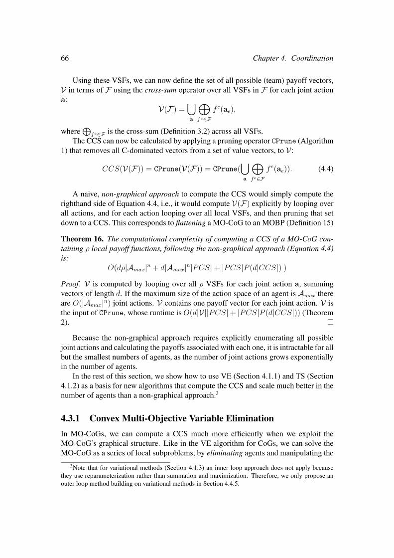
66 Chapter 4. Coordination
Using these VSFs, we can now define the set of all possible (team) payoff vectors,V in terms of F using the cross-sum operator over all VSFs in F for each joint actiona:
V(F) =⋃a
⊕fe∈F
f e(ae),
where⊕
fe∈F is the cross-sum (Definition 3.2) across all VSFs.The CCS can now be calculated by applying a pruning operator CPrune (Algorithm
1) that removes all C-dominated vectors from a set of value vectors, to V:
CCS(V(F)) = CPrune(V(F)) = CPrune(⋃a
⊕fe∈F
f e(ae)). (4.4)
A naive, non-graphical approach to compute the CCS would simply compute therighthand side of Equation 4.4, i.e., it would compute V(F) explicitly by looping overall actions, and for each action looping over all local VSFs, and then pruning that setdown to a CCS. This corresponds to flattening a MO-CoG to an MOBP (Definition 15)
Theorem 16. The computational complexity of computing a CCS of a MO-CoG con-taining ρ local payoff functions, following the non-graphical approach (Equation 4.4)is:
O(dρ|Amax|n + d|Amax|n|PCS|+ |PCS|P (d|CCS|) )
Proof. V is computed by looping over all ρ VSFs for each joint action a, summingvectors of length d. If the maximum size of the action space of an agent is Amax thereare O(|Amax|n) joint actions. V contains one payoff vector for each joint action. V isthe input of CPrune, whose runtime is O(d|V||PCS|+ |PCS|P (d|CCS|)) (Theorem2).
Because the non-graphical approach requires explicitly enumerating all possiblejoint actions and calculating the payoffs associated with each one, it is intractable for allbut the smallest numbers of agents, as the number of joint actions grows exponentiallyin the number of agents.
In the rest of this section, we show how to use VE (Section 4.1.1) and TS (Section4.1.2) as a basis for new algorithms that compute the CCS and scale much better in thenumber of agents than a non-graphical approach.3
4.3.1 Convex Multi-Objective Variable EliminationIn MO-CoGs, we can compute a CCS much more efficiently when we exploit theMO-CoG’s graphical structure. Like in the VE algorithm for CoGs, we can solve theMO-CoG as a series of local subproblems, by eliminating agents and manipulating the
3Note that for variational methods (Section 4.1.3) an inner loop approach does not apply becausethey use reparameterization rather than summation and maximization. Therefore, we only propose anouter loop method building on variational methods in Section 4.4.5.

4.3. Inner Loop CCS Methods for MO-CoGs 67
set of VSFs F which describe the MO-CoG. We call the resulting algorithm ConvexMulti-Objective Variable Elimination (CMOVE). CMOVE is an extension to Rollonand Larrosa’s Pareto-based extension of VE, which we refer to as PMOVE (Rollonand Larrosa, 2006).
The key idea of CMOVE is to compute local CCSs (LCCSs) when eliminating anagent instead of a single best response (as in VE). When computing an LCCS, thealgorithm prunes away as many vectors as possible, minimizing the number of payoffvectors that are calculated at the global level. Minimizing the number of payoff vectorsthat are calculated greatly reduces computation time.
Eliminating agents
First, we describe the elim operator for eliminating agents from a set of VSF. Thisoperator corresponds to the elim operator used by VE (Algorithm 9) for eliminatingagents in single-objective CoGs. We first need to update our definition of neighboringlocal payoff functions (Definition 23), to neighboring VSFs.
Definition 28. The set of neighboring VSFsFi of i is the set of all local payoff functionsthat have agent i in scope.
The neighboring agents ni of an agent i are now the agents in the scope of a VSF inFi, except for i itself, corresponding to Definition 24. For each possible local jointaction of ni, we now compute an LCCS — a local CCS — that contains the payoffsof the C-undominated responses of agent i, as the best response values of i. In otherwords, it is the CCS of the subproblem that arises when considering only Fi and fixinga specific local joint action ani .
To compute the LCCS, we must consider all payoff vectors of the subproblem, Vi,and prune the C-dominated ones. This can be achieved by taking the cross-sum of allthe VSFs in the local subproblem, and then pruning.
Definition 29. If we fix all actions in ani , but not ai, the set of all payoff vectors is:Vi(Fi, ani) =
⋃ai
⊕fe∈Fi f
e(ae), where ae is formed from ai and the appropriate partof ani .
Using Definition 29, we can now formally define the LCCS as the CCS of Vi:
Definition 30. A local CCS, an LCCS, is the C-undominated subset of Vi(Fi, ani):
LCCSi(Fi, ani) = CCS(Vi(Fi, ani)).
Because the LCCSi is the CCS of a specified set of vectors, we can compute theLCCS by standard pruning algorithms, such as CPrune (Algorithm 1). Using LCCSs,we can create a new VSF, fnew, conditioned on the actions of the agents in ni:
∀ani fnew(ani) = LCCSi(Fi, ani).

68 Chapter 4. Coordination
The elim operator replaces the VSFs in Fi in F by this new factor:
elim(F , i) = (F \ Fi) ∪ fnew(ani).
Eliminating an agent reduces the number of agents and VSFs in the graph, andforms the cornerstone operator of the CMOVE algorithm. Before defining the fullCMOVE algorithm, we first prove the correctness of elim. Particularly (as describedin Section 3.1.1), we must prove that no necessary vectors are lost when applying theelim operator.
We show that the maximal scalarized payoff, for any w, cannot be lost as a resultof elim, i.e., no necessary payoff vectors for creating a CCS are lost.
Theorem 17. elim preserves the CCS, i.e.,
∀i ∀F CCS(V(F)) = CCS(V(elim(F , i))).
Proof. By definition the CCS of a MO-CoG, contains at least one payoff vector thatmaximizes the scalarized value for every w. Therefore, for each vector u(a) that isoptimal for at least one w, there must be a vector that achieves the same scalarizedvalue for that w:
∀w(a = arg max
a∈Aw · u(a)
)=⇒
∃a′ u(a′) ∈ CCS(V(F)) ∧ w · u(a) = w · u(a′). (4.5)
If and only if this is not the case, necessary values are lost.First, we observe that for all joint actions a for which there is a w at which the
scalarized value of a is maximal, a vector-valued payoff u(a′) for which w · u(a′) =w ·u(a) is in the CCS (by definition). Second, we observe that the linear scalarizationfunction distributes over the local payoff functions: w · u(a) = w ·
∑e u
e(ae) =∑ew · ue(ae). Thus, when eliminating agent i, we divide the set of VSFs into non-
neighbors (nn), in which agent i does not participate, and neighbors (ni) such that:
w · u(a) =∑e∈nn
w · ue(ae) +∑e∈ni
w · ue(ae).
Now, following Equation 4.5, the CCS contains maxa∈Aw · u(a) for all w. elimpushes this maximization in:
maxa∈A
w · u(a) = maxa−i∈A−i
∑e∈nn
w · ue(ae) + maxai∈Ai
∑e∈ni
w · ue(ae).
elim replaces the agent-i factors by a term fnew(ani) that satisfies w · fnew(ani) =maxai
∑e∈ni w · u
e(ae) — for all w — per definition, thus preserving the maximumscalarized value for all w and thereby preserving the CCS.

4.3. Inner Loop CCS Methods for MO-CoGs 69
Instead of an LCCS, we could compute a local PCS (LPCS), that is, using a PCScomputation on Vi instead of a CCS computation. Note that, since LCCS ⊆ LPCS⊆ Vi, elim not only reduces the problem size with respect to Vi, it can do so morethan would be possible if we only considered P-dominance. Therefore, focusing onthe CCS can greatly reduce the sizes of local subproblems. Since the solution of alocal subproblem is the input for the next agent elimination, the size of subsequentlocal subproblems is also reduced, which can lead to considerable speed-ups.
Algorithm
Using elim, we now present the convex multi-objective variable elimination (CMOVE)algorithm. In our implementation elim uses CPrune to compute the local CCSs. LikeVE, CMOVE iteratively eliminates agents until none are left. However, our implemen-tation of elim computes a CCS and outputs the correct joint actions for each payoffvector in this CCS, rather than a single joint action.
As previously mentioned, CMOVE is an extension to Rollon and Larrosa’s Pareto-based extension of VE, which we refer to as PMOVE (Rollon and Larrosa, 2006). Themost important difference between CMOVE and PMOVE is that CMOVE computes aCCS, which typically leads to much smaller subproblems and thus much better compu-tational efficiency. In addition, we identify three places where pruning can take place,yielding a more flexible algorithm with different trade-offs. Finally, we use the taggingscheme instead of the backwards pass, as in Section 4.1.1.
Algorithm 10 presents an abstract version of CMOVE that leaves the pruning op-erators unspecified. Depending on preference, these pruning operators can be filled inwith PPrune (Algorithm 2), or CPrune (Algorithm 1), or other algorithms for comput-ing PCSs or CCSs. Depending on which pruning operators are used in which points inthe algorithm, Algorithm 10 correctly computes a correct CCS or PCS.4
CMOVE first translates the problem into a set of vector-set factors (VSFs), F online 1, according to Equation 4.3. Next, CMOVE iteratively eliminates agents usingelim (line 2–5). The elimination order can be determined using techniques devised forsingle-objective VE (e.g., the method proposed by Koller and Friedman (2009) for thispurpose).
Algorithm 11 shows our implementation of elim, parameterized with two pruningoperators, prune1 and prune2. These pruning operators correspond to two differentpruning locations inside the operator that computes LCCSi: ComputeLCCSi(Fi, ani ,prune1, prune2).
4If more information is known about the scalarization function, f (Definition 1), this could be incor-porated in new pruning algorithms, that could be used here as well. E.g., if it is known that objective1 is worth as least twice as much as objective 2, inside a linear scalarization function, this could beincorporated into the pruning operators, without affecting the correctness of the algorithm. However,what is possible in this respect highly depends on what information about f is available, and is beyondthe scope of this dissertation.
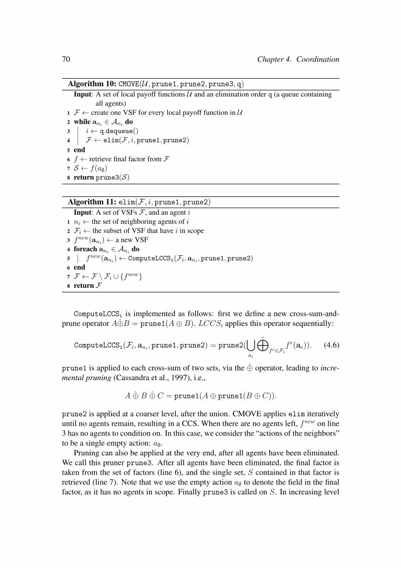
70 Chapter 4. Coordination
Algorithm 10: CMOVE(U , prune1, prune2, prune3, q)
Input: A set of local payoff functions U and an elimination order q (a queue containingall agents)
1 F ← create one VSF for every local payoff function in U2 while ani ∈ Ani do3 i← q.dequeue()4 F ← elim(F , i, prune1, prune2)
5 end6 f ← retrieve final factor from F7 S ← f(a∅)8 return prune3(S)
Algorithm 11: elim(F , i, prune1, prune2)
Input: A set of VSFs F , and an agent i1 ni ← the set of neighboring agents of i2 Fi ← the subset of VSF that have i in scope3 fnew(ani)← a new VSF4 foreach ani ∈ Ani do5 fnew(ani)← ComputeLCCSi(Fi,ani , prune1, prune2)6 end7 F ← F \ Fi ∪ fnew8 return F
ComputeLCCSi is implemented as follows: first we define a new cross-sum-and-prune operator A⊕B = prune1(A⊕B). LCCSi applies this operator sequentially:
ComputeLCCSi(Fi, ani , prune1, prune2) = prune2(⋃ai
⊕fe∈Fi
f e(ae)). (4.6)
prune1 is applied to each cross-sum of two sets, via the ⊕ operator, leading to incre-mental pruning (Cassandra et al., 1997), i.e.,
A ⊕ B ⊕ C = prune1(A⊕ prune1(B ⊕ C)).
prune2 is applied at a coarser level, after the union. CMOVE applies elim iterativelyuntil no agents remain, resulting in a CCS. When there are no agents left, fnew on line3 has no agents to condition on. In this case, we consider the “actions of the neighbors”to be a single empty action: a∅.
Pruning can also be applied at the very end, after all agents have been eliminated.We call this pruner prune3. After all agents have been eliminated, the final factor istaken from the set of factors (line 6), and the single set, S contained in that factor isretrieved (line 7). Note that we use the empty action a∅ to denote the field in the finalfactor, as it has no agents in scope. Finally prune3 is called on S. In increasing level

4.3. Inner Loop CCS Methods for MO-CoGs 71
of coarseness, we thus have three pruning operators: incremental pruning (prune1),pruning after the union over actions of the eliminated agent (prune2), and pruningafter all agents have been eliminated (prune3).
When either prune2 or prune3 (or both) compute CCSs, the CMOVE algorithmscorrectly computes the CCS. When no pruning takes place for prune3 and prune1 =prune2 = PPrune, the resulting algorithm computes the PCS rather than the CCS, andis equivalent to the PMOVE algorithm proposed by Rollon and Larrosa (2006).
When comparing CMOVE to PMOVE we make the following observation: thelocal coverage sets are input to the next subproblem in agent elimination sequence.A smaller local coverage set thus results in a smaller next subproblem. Because it isalways possible to have a CCS that is a subset of the smallest possible PCS, the sub-problems in CMOVE are thus always smaller than the corresponding subproblems inPMOVE. A key insight behind CMOVE is that this results in faster computation over-all for CMOVE compared to PMOVE. Furthermore, we discuss variants of CMOVE,with different instantiations of the pruning operators, that lead to different trade-offsbetween pruning and the size of the subproblems.
CMOVE Variants
There are several ways to implement the pruning operators that lead to correct instan-tiations of CMOVE. Both PPrune (Algorithm 2) and CPrune (Algorithm 1) can beused, as long as either prune2 or prune3 is CPrune. Note that if prune2 computesthe CCS, prune3 is not necessary.
In this dissertation, we consider two variants: Basic CMOVE, which does notuse prune1 and prune3 and only prunes at prune2 using CPrune, and IncrementalCMOVE, which uses CPrune at both prune1 and prune2. The latter invests moreeffort in intermediate pruning, which can result in smaller cross-sums, and a result-ing speedup. However, when only a few vectors can be pruned in these intermediatesteps, this additional speedup may not occur, and the algorithm creates unnecessaryoverhead.5
Example
Consider the example in Figure 4.1a, using the payoffs defined by Table 4.2, and applyCMOVE, using CPrune for prune2, and no pruning for prune1 and prune3, i.e., BasicCMOVE.
First, CMOVE creates the VSFs f 1 and f 2 from u1 and u2. To eliminate agent3, it creates a new VSF f 3(a2) by computing the LCCSs for every a2 and taggingeach element of each set with the action of agent 3 that generates it. For a2, CMOVEfirst generates the set (3, 1)a3 , (1, 3)a3. Since both of these vectors are optimal for
5We can also compute a PCS first, using prune1 and prune2, and then compute the CCS withprune3. However, this is useful only for small problems for which a PCS is cheaper to compute than aCCS.

72 Chapter 4. Coordination
some w, neither is removed by pruning and thus f 3(a2) = (3, 1)a3 , (1, 3)a3. For a2,CMOVE first generates (0, 0)a3 , (1, 1)a3. CPrune determines that (0, 0)a3 is domi-nated and consequently removes it, yielding f 3(a2) = (1, 1)a3. CMOVE then addsf 3 to the graph and removes f 2 and agent 3, yielding the factor graph shown in Figure4.1b.
CMOVE then eliminates agent 2 by combining f 1 and f 3 to create f 4. For f 4(a1),CMOVE must calculate the LCCS of:
(f 1(a1, a2)⊕ f 3(a2)) ∪ (f 1(a1, a2)⊕ f 3(a2)).
The first cross sum yields (7, 2)a2a3 , (5, 4)a2a3 and the second yields (1, 1)a2a3.Pruning their union yields f 4(a1) = (7, 2)a2a3 , (5, 4)a2a3. Similarly, for a1 tak-ing the union yields (4, 3)a2a3 , (2, 5)a2a3 , (4, 7)a2a3, of which the LCCS is f 4(a1) =(4, 7)a2a3. Adding f 4 results in the graph in Figure 4.1c.
Finally, CMOVE eliminates agent 1. Since there are no neighboring agents left,Ai contains only the empty action. CMOVE takes the union of f 4(a1) and f 4(a1).Since (7, 2)a1a2a3 and (4, 7)a1a2a3 dominate (5, 4)a1a2a3, the latter is pruned, leav-ing CCS = (7, 2)a1a2a3, (4, 7)a1a2a3.
Analysis
We now analyze the correctness and complexity of CMOVE.
Theorem 18. CMOVE correctly computes a CCS.
Proof. The proof works by induction on the number of agents. The base case is theoriginal MO-CoG, where each f e(ae) from F is a singleton set. Then, since elim
preserves the CCS (see Theorem 17), no necessary vectors are lost. Furthermore, noexcess payoff vectors are retained; when the last agent is eliminated, only one factorremains; since it is not conditioned on any agent actions and is the result of an LCCScomputation, it must contain one set: the CCS.
Theorem 19. The computational complexity of CMOVE is
O( n |Amax|wa (wf R1 +R2) +R3 ), (4.7)
where wa is the induced agent width, i.e., the maximum number of neighboring agents(connected via factors) of an agent when eliminated, wf is the induced factor width,i.e., the maximum number of neighboring factors of an agent when eliminated, and R1,R2 and R3 are the cost of applying the prune1, prune2 and prune3 operators.
Proof. CMOVE eliminates n agents and for each one computes an LCCS for eachjoint action of the eliminated agent’s neighbors, in a field in a new VSF. CMOVEcomputes O(|Amax|wa) fields per iteration, calling prune1 (Equation 4.6) for eachadjacent factor, and prune2 once after taking the union over actions of the eliminatedagent. prune3 is called exactly once, after eliminating all agents (line 8 of Algorithm10).
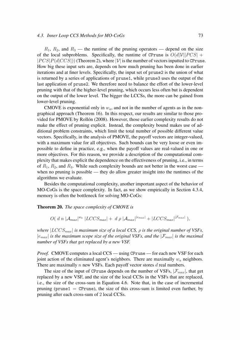
4.3. Inner Loop CCS Methods for MO-CoGs 73
R1, R2, and R3 — the runtime of the pruning operators — depend on the sizeof the local subproblems. Specifically, the runtime of CPrune is O(d|V||PCS| +|PCS|P (d|CCS|)) (Theorem 2), where |V| is the number of vectors inputted to CPrune.How big these input sets are, depends on how much pruning has been done in earlieriterations and at finer levels. Specifically, the input set of prune2 is the union of whatis returned by a series of applications of prune1, while prune3 uses the output of thelast application of prune2. We therefore need to balance the effort of the lower-levelpruning with that of the higher-level pruning, which occurs less often but is dependenton the output of the lower level. The bigger the LCCSs, the more can be gained fromlower-level pruning.
CMOVE is exponential only in wa, and not in the number of agents as in the non-graphical approach (Theorem 16). In this respect, our results are similar to those pro-vided for PMOVE by Rollon (2008). However, those earlier complexity results do notmake the effect of pruning explicit. Instead, the complexity bound makes use of ad-ditional problem constraints, which limit the total number of possible different valuevectors. Specifically, in the analysis of PMOVE, the payoff vectors are integer-valued,with a maximum value for all objectives. Such bounds can be very loose or even im-possible to define in practice, e.g., when the payoff values are real-valued in one ormore objectives. For this reason, we provide a description of the computational com-plexity that makes explicit the dependence on the effectiveness of pruning, i.e., in termsof R1, R2, and R3. While such complexity bounds are not better in the worst case —when no pruning is possible — they do allow greater insight into the runtimes of thealgorithms we evaluate.
Besides the computational complexity, another important aspect of the behavior ofMO-CoGs is the space complexity. In fact, as we show empirically in Section 4.3.4,memory is often the bottleneck for solving MO-CoGs:
Theorem 20. The space complexity of CMOVE is
O( d n |Amax|wa |LCCSmax|+ d ρ |Amax||emax| + |LCCSmax||Fmax| ),
where |LCCSmax| is maximum size of a local CCS, ρ is the original number of VSFs,|emax| is the maximum scope size of the original VSFs, and the |Fmax| is the maximalnumber of VSFs that get replaced by a new VSF.
Proof. CMOVE computes a local CCS — using CPrune — for each new VSF for eachjoint action of the eliminated agent’s neighbors. There are maximally wa neighbors.There are maximally n new VSFs. Each payoff vector stores d real numbers.
The size of the input of CPrune depends on the number of VSFs, |Fmax|, that getreplaced by a new VSF, and the size of the local CCSs in the VSFs that are replaced,i.e., the size of the cross-sum in Equation 4.6. Note that, in the case of incrementalpruning (prune1 = CPrune), the size of this cross-sum is limited even further, bypruning after each cross-sum of 2 local CCSs.

74 Chapter 4. Coordination
There are ρ VSFs created during the initialization of CMOVE. All of these VSFshave exactly one payoff vector containing d real numbers, per joint action of the agentsin scope. There are maximally |Amax||emax| such joint actions.
For PMOVE, the space complexity is equivalent to Theorem 20, but with the size ofa local PCS, |LPCSmax|, instead of |LCCSmax|. Because an LCCS is a subset of thecorresponding LPCS6, CMOVE is thus strictly more memory efficient than PMOVE.
Note that Theorem 20 is a rather loose upper bound on the space complexity, asnot all VSFs, original or new, exist at the same time. However, it is not possible to topredict a priori how many of these VSFs exist at the same time, resulting in a spacecomplexity bound on the basis of all VSFs that exist at some point during the executionof CMOVE.
4.3.2 Experiments: CMOVE versus PMOVEIn order to test the efficiency of CMOVE, we compare basic CMOVE and incrementalCMOVE to PMOVE7 and the non-graphical approach (described at the beginning ofSection 4.3) for problems with varying numbers of agents and objectives. We alsoanalyze how these runtimes correspond to the sizes of the PCS and CCS, as well as theinduced width.
Because CMOVE and PMOVE are inner loop methods based on the same schema,i.e., VE, these experiments indicate how inner loop methods that compute the CCScompare to inner loop methods that compute the CCS. Furthermore, we see how thedifferent variants of CMOVE compare to each other.
We use two types of experiments. The first experiments are done with randomMO-CoGs in which we can directly control all variables. In the second experiment,we use Mining Day, a more realistic benchmark, that is more structured than randomMO-CoGs but still randomized.
Random Graphs
To generate random MO-CoGs, we employ a procedure that takes as input: n, thenumber of agents; d, the number of payoff dimensions; ρ the number of local payofffunctions; and |Ai|, the action space size of the agents, which is the same for all agents.The procedure then starts with a fully connected graph with local payoff functionsconnecting to two agents each. Then, local payoff functions are randomly removed,while ensuring that the graph remains connected, until only ρ local payoff functionsremain. The values for the different objectives in each local payoff function are realnumbers that are drawn independently and uniformly from the interval [0, 10].
6Our implementation of CPrune (Algorithm 1) uses PPrune as a pre-processing step (on line 1).7We compare to PMOVE using only prune2 = PPrune, rather than prune1 = prune2 = PPrune,
as was proposed in the original article (Rollon and Larrosa, 2006) because we found the former optionslightly but consistently faster.

4.3. Inner Loop CCS Methods for MO-CoGs 75
20 40 60 80
1100
10000
number of agents
runtime(ms)
non-graphicalPMOVEbasic CMOVEincr. CMOVE
20 30 40 50 60 70
050
150
number of agents
set s
ize
PCS sizeCCS size
15 30 45 60
456789
11
number of agents
indu
ced
wid
th
(a) (b) (c)
Figure 4.4: (a) Runtimes (ms) in log-scale for the nongraphical method, PMOVE and CMOVEwith standard deviation of mean (error bars), (b) the corresponding number of vectors in thePCS and CCS, and (c) the corresponding spread of the induced width as a boxplot.
We compare algorithms on the same set of randomly generated MO-CoGs for eachseparate value of n, d, ρ, and |Ai|.
To compare basic CMOVE, incremental CMOVE, PMOVE, and the non-graphicalmethod, we test them on random MO-CoGs with the number of agents ranging between10 and 85, the average number of factors per agent held at ρ = 1.5n, and the numberof objectives d = 2. This experiment was run on a 2.4 GHz Intel Core i5 computer,with 4 GB memory. Figure 4.4 shows the results, averaged over 20 MO-CoGs foreach number of agents. The runtime (Figure 4.4a) of the non-graphical method quicklyexplodes. Both CMOVE variants are slower than PMOVE for small numbers of agents,but the runtime grows much more slowly than that of PMOVE. At 70 agents, bothCMOVE variants are faster than PMOVE on average. For 75 agents, one of the MO-CoGs generated caused PMOVE to time out at 5000s, while basic CMOVE had amaximum runtime of 132s, and incremental CMOVE 136s. This can be explained bythe differences in the size of the solutions, i.e., the PCS and the CCS (Figure 4.4b). ThePCS grows much more quickly with the number of agents than the CCS does. For two-objective problems, incremental CMOVE seems to be consistently slower than basicCMOVE.
While CMOVE’s runtime grows much more slowly than that of the nongraphicalmethod, it is still exponential in the number of agents, a counterintuitive result sincethe worst-case complexity is linear in the number of agents. This can be explained bythe induced width of the MO-CoGs, in which the runtime of CMOVE is exponential.In Figure 4.4c, we see that the induced width increases linearly with the number ofagents for random graphs.
We therefore conclude that, in two-objective MO-CoGs, the non-graphical methodis intractable, even for small numbers of agents, and that the runtime of CMOVE in-creases much less with the number of agents than PMOVE does.
To test how the runtime behavior changes with a higher number of objectives, werun the same experiment with the average number of factors per agent held at ρ = 1.5nand increasing numbers of agents again, but now for d = 5. This and all remain-ing experiments described in this section were executed on a Xeon L5520 2.26 GHz

76 Chapter 4. Coordination
10 15 20 25 30
1e+02
1e+04
1e+06
number of agents
dag[
, 5]
non-graphicalPMOVEbasic CMOVEincr. CMOVE
2 3 4 5 6 7 8
1e+01
1e+03
1e+05
number of dimensions
set s
ize
PCS sizeCCS size
Figure 4.5: Runtimes (ms) for the non-graphical method, PMOVE and CMOVE in log-scalewith the standard deviation of mean (error bars) (left) and the corresponding number of vectorsin the PCS and CCS (right), for increasing numbers of agents and 5 objectives.
computer with 24 GB memory. Figure 4.5 (left) shows the results of this experiment,averaged over 85 MO-CoGs for each number of agents. Note that we do not plotthe induced widths, as this does not change with the number of objectives. These re-sults demonstrate that, as the number of agents grows, using CMOVE becomes keyto containing the computational cost of solving the MO-CoG. CMOVE outperformsthe nongraphical method from 12 agents onwards. At 25 agents, basic CMOVE is 38times faster. CMOVE also does significantly better than PMOVE. Though it is oneorder of magnitude slower with 10 agents (238ms (basic) and 416ms (incremental)versus 33ms on average), its runtime grows much more slowly than that of PMOVE.At 20 agents, both CMOVE variants are faster than PMOVE and at 28 agents, BasicCMOVE is almost one order of magnitude faster (228s versus 1, 650s on average), andthe difference increases with every agent.
As before, the runtime of CMOVE is exponential in the induced width, whichincreases with the number of agents, from 3.1 at n = 10 to 6.0 at n = 30 on average,as a result of the random MO-CoG generation procedure. However, CMOVE’s runtimeis polynomial in the size of the CCS, and this size grows exponentially, as shown inFigure 4.5 (right). The fact that CMOVE is much faster than PMOVE can be explainedby the sizes of the PCS and CCS, as the former grows much faster than the latter. At10 agents, the average PCS size is 230 and the average CCS size is 65. At 30 agents,the average PCS size has risen to 51, 745 while the average CCS size is only 1, 575.
Figure 4.6 (left) compares the scalability of the algorithms in the number of objec-tives, on random MO-CoGs with n = 20 and ρ = 30, averaged over 100 MO-CoGs.CMOVE always outperforms the nongraphical method. Interestingly, the nongraphicalmethod is several orders of magnitude slower at d = 2, grows slowly until d = 5, andthen starts to grow with about the same exponent as PMOVE. This can be explainedby the fact that the time it takes to enumerate of all joint actions and payoffs remainsapproximately constant, while the time it takes to prune increases exponentially withthe number of objectives. When d = 2, CMOVE is an order of magnitude slower thanPMOVE (163ms (basic) and 377 (incremental) versus 30ms). However, when d = 5,

4.3. Inner Loop CCS Methods for MO-CoGs 77
2 3 4 5 6 7 8
1e+02
1e+04
1e+06
number of objectives
runtime(ms)
non-graphicalPMOVEbasic CMOVEincr. CMOVE
2 3 4 5 6 7
550
50010000
number of dimensions
set s
ize
PCS sizeCCS size
Figure 4.6: Runtimes (ms) for the non-graphical method, PMOVE and CMOVE in logscalewith the standard deviation of mean (error bars) (left) and the corresponding number of vectorsin the PCS and CCS (right), for increasing numbers of objectives.
both CMOVE variants are already faster than PMOVE and at 8 dimensions they arerespectively 3.2 and 2.4 times faster. This happens because the CCS grows much moreslowly than the PCS, as shown in Figure 4.6 (right). The difference between incremen-tal and basic CMOVE decreases as the number of dimensions increases, from a factor2.3 at d = 2 to 1.3 at d = 8. This trend indicates that pruning after every cross-sum,i.e., at prune1, becomes (relatively) better for higher numbers of objectives. Althoughwe were unable to solve problem instances with many more objectives within reason-able time, we expect this trend to continue and that incremental CMOVE would befaster than basic CMOVE for problems with very many objectives.
Overall, we conclude that, for random graphs, CMOVE is key to solving MO-CoGs within reasonable time, especially when the problem size increases in either thenumber of agents, the number of objectives, or both.
Mining Day
In Mining Day, a mining company mines gold and silver (objectives) from a set ofmines (local payoff functions) located in the mountains (see Figure 1.2). The mineworkers live in villages at the foot of the mountains. The company has one van in eachvillage (agents) for transporting workers and must determine every morning to whichmine each van should go (actions). However, vans can only travel to nearby mines(graph connectivity). Workers are more efficient if there are more workers at the mine:there is a 3% efficiency bonus per worker such that the amount of each resource minedper worker is x · 1.03w, where x is the base rate per worker and w is the number ofworkers at the mine. The base rate of gold and silver are properties of a mine. Sincethe company aims to maximize revenue, the best strategy depends on the fluctuatingprices of gold and silver. To maximize revenue, the mining company wants to use thelatest possible price information, and not lose time recomputing the optimal strategy

78 Chapter 4. Coordination
20 60 100
010000
20000
number of agents
runtime(ms)
Basic CMOVEIncr. CMOVEPMOVE
20 60 100
0200
600
1000
number of agents
set s
ize
PCS sizeCCS size
Figure 4.7: Runtimes (ms) for basic and incremental CMOVE, and PMOVE, in log-scale withthe standard deviation of mean (error bars) (left) and the corresponding number of vectors inthe PCS and CCS (right), for increasing numbers of agents.
with every price change. Therefore, we must calculate a CCS.To generate a Mining Day instance with v villages (agents), we randomly assign
2-5 workers to each village and connect it to 2-4 mines. Each village is only connectedto mines with a greater or equal index, i.e., if village i is connected to m mines, it isconnected to mines i to i + m − 1. The last village is connected to 4 mines and thusthe number of mines is v+ 3. The base rates per worker for each resource at each mineare drawn uniformly and independently from the interval [0, 10].
In order to compare the runtimes of basic and incremental CMOVE against PMOVEon a more realistic benchmark, we generate Mining Day instances with varying num-bers of agents. Note that we do not include the non-graphical method, as its runtimemainly depends on the number of agents, and is thus not considerably faster for thisproblem than for random graphs. The runtime results are shown in Figure 4.7 (left).Both CMOVE and PMOVE are able to tackle problems with over 100 agents. However,the runtime of PMOVE grows much more quickly than that of CMOVE. In this two-objective setting, basic CMOVE is better than incremental CMOVE. Basic CMOVEand PMOVE both have runtimes of around 2.8s at 60 agents, but at 100 agents, basicCMOVE runs in about 5.9s and PMOVE in 21s. Even though incremental CMOVEis worse than basic CMOVE, its runtime still grows much more slowly than that ofPMOVE, and it beats PMOVE when there are many agents.
The difference between PMOVE and CMOVE results from the relationship be-tween the number of agents and the sizes of the CCS, which grows linearly, and thePCS, which grows polynomially, as shown in Figure 4.7 (right). The induced widthremains around 4 regardless of the number of agents. These results demonstrate that,as the CCS grows more slowly than the PCS with the number of agents, CMOVE cansolve MO-CoGs more efficiently than PMOVE as the number of agents increases.
From these — as well as the Random Graphs results — we conclude that CMOVE
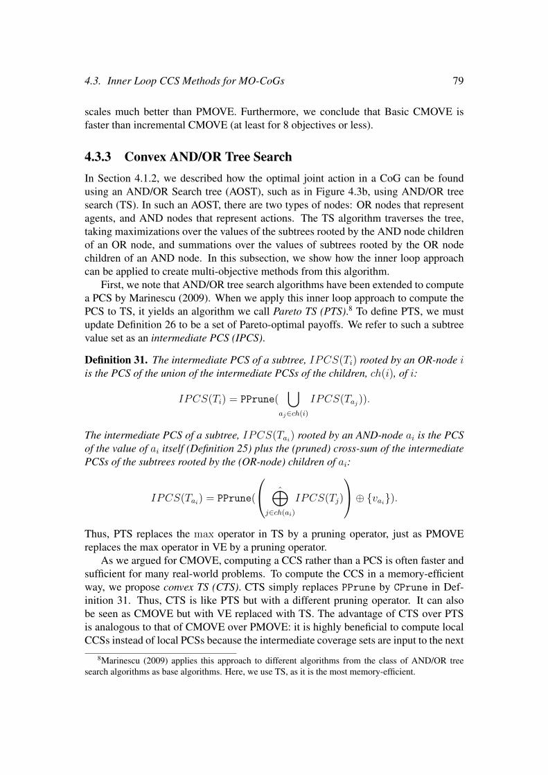
4.3. Inner Loop CCS Methods for MO-CoGs 79
scales much better than PMOVE. Furthermore, we conclude that Basic CMOVE isfaster than incremental CMOVE (at least for 8 objectives or less).
4.3.3 Convex AND/OR Tree SearchIn Section 4.1.2, we described how the optimal joint action in a CoG can be foundusing an AND/OR Search tree (AOST), such as in Figure 4.3b, using AND/OR treesearch (TS). In such an AOST, there are two types of nodes: OR nodes that representagents, and AND nodes that represent actions. The TS algorithm traverses the tree,taking maximizations over the values of the subtrees rooted by the AND node childrenof an OR node, and summations over the values of subtrees rooted by the OR nodechildren of an AND node. In this subsection, we show how the inner loop approachcan be applied to create multi-objective methods from this algorithm.
First, we note that AND/OR tree search algorithms have been extended to computea PCS by Marinescu (2009). When we apply this inner loop approach to compute thePCS to TS, it yields an algorithm we call Pareto TS (PTS).8 To define PTS, we mustupdate Definition 26 to be a set of Pareto-optimal payoffs. We refer to such a subtreevalue set as an intermediate PCS (IPCS).
Definition 31. The intermediate PCS of a subtree, IPCS(Ti) rooted by an OR-node iis the PCS of the union of the intermediate PCSs of the children, ch(i), of i:
IPCS(Ti) = PPrune(⋃
aj∈ch(i)
IPCS(Taj)).
The intermediate PCS of a subtree, IPCS(Tai) rooted by an AND-node ai is the PCSof the value of ai itself (Definition 25) plus the (pruned) cross-sum of the intermediatePCSs of the subtrees rooted by the (OR-node) children of ai:
IPCS(Tai) = PPrune(
⊕j∈ch(ai)
IPCS(Tj)
⊕ vai).Thus, PTS replaces the max operator in TS by a pruning operator, just as PMOVEreplaces the max operator in VE by a pruning operator.
As we argued for CMOVE, computing a CCS rather than a PCS is often faster andsufficient for many real-world problems. To compute the CCS in a memory-efficientway, we propose convex TS (CTS). CTS simply replaces PPrune by CPrune in Def-inition 31. Thus, CTS is like PTS but with a different pruning operator. It can alsobe seen as CMOVE but with VE replaced with TS. The advantage of CTS over PTSis analogous to that of CMOVE over PMOVE: it is highly beneficial to compute localCCSs instead of local PCSs because the intermediate coverage sets are input to the next
8Marinescu (2009) applies this approach to different algorithms from the class of AND/OR treesearch algorithms as base algorithms. Here, we use TS, as it is the most memory-efficient.

80 Chapter 4. Coordination
subproblem in a sequential search scheme, regardless of whether that scheme is VE orTS; this is both more runtime and memory efficient.
Like in CMOVE, we can apply incremental pruning (Cassandra et al., 1997), i.e.,pruning after every cross-sum. Incremental pruning is more memory efficient, as itgreatly reduces the sizes of the cross-sums.
While CTS is more memory efficient than CMOVE, it still requires computingintermediate coverage sets that take up space. While these are typically only about aslarge as the CCS, their size is bounded only by the total number of joint actions.
Analysis
Using the time and space complexity results for TS, we can establish the followingcorollaries about the time and space complexity of CTS.
Corollary 4. The time complexity of CTS is O(n|Amax|mR), where R is the runtimeof CPrune.
Proof. O(n|Amax|m) bounds the number of nodes in the AOST. For each node in theAOST CPrune is called.
The runtime of CPrune in terms of the size of its input is given by Definition 2.The size of the input of CPrune depends on the size of the intermediate CCSs of thechildren of a node. In the case of an AND-node, this input size is O(|ICCSmax|c),where c is the maximum number of children of an AND-node.9 For OR-nodes this isO(|Amax||ICCSmax|).
Corollary 5. The space complexity of CTS is
O(n|ICCSmax|+ |Amax||ICCSmax|+ |ICCSmax|c),
where |ICCSmax| is the maximum size of an intermediate CCS during the executionof CTS.
Proof. Like in TS, only O(n) nodes of the AOST need to exist during any point duringexecution, and each node contains an intermediate CCS. After computing a cross-sumat most |ICCSmax|c vectors are generated before pruning.
Note that when incremental pruning is applied, the full cross-sums (of size |ICCSmax|c)are never generated. Instead, the cross-sums of only 2 (instead of c) ICCSs are com-puted. CTS is much more memory efficient than CMOVE, which has a space com-plexity that is exponential in the induced width (Theorem 20).
9Note that c is in turn upper bounded by n but this is a very loose bound.

4.3. Inner Loop CCS Methods for MO-CoGs 81
10 20 30 40
1e+00
1e+04
number of agents
runt
ime
(ms)
CTSPTSCMOVEPMOVE
10 20 30 40
0500
1000
1500
number of agentsse
t siz
e
CCSPCS
10 20 30 40
46
810
1214
number of agents
indu
ced
wid
th
Figure 4.8: (left) Runtimes in ms of CTS, basic CMOVE and PMOVE on random3-objective MO-CoGs with varying numbers of agents n and ρ = 2.0n local payofffactors. (right) The corresponding CCS and PCS sizes of the MO-CoGs. (right) Thecorresponding induced widths of the MO-CoGs.
4.3.4 Experiments: CTS versus CMOVE
In this subsection we empirically compare CMOVE and CTS in settings where thereis little available memory. In order to test the memory-efficiency, we limit the memorythe algorithms is allowed to use, using the -Xmx runtime option for the JAVA VirtualMachine. All experiments use our JAVA implementation (version 1.6 SE), and thecorresponding MacOS X Virtual Machine. All experiments in this subsection were runon a 2.4 GHz Intel Core i5 computer, with 4 GB memory.
To obtain the PTs for CTS, we use the same heuristic as CMOVE and VELS togenerate an elimination order. We then transform this elimination order into a PT forwhich m ≤ w log n holds (whose existence is guaranteed by Theorem 15), using theprocedure suggested by Bayardo and Miranker .
We employ the same generation procedure for random graphs as in Section 4.3.2.Because connections between agents in these graphs are generated randomly, the in-duced width varies between different problems. On average, the induced width in-creases with the number of local payoff functions, even when the ratio between localpayoff factors and the number of agents remains constant.
In order to test the sizes of problems that the different MO-CoG solution methodscan handle within limited memory, we generate very challenging random graphs witha varying number of agents n, three objectives, and ρ = 2.0n local payoff functions.We limited the maximal available memory to 10MB.
Figure 4.8 (left) shows that within 10 MB, PMOVE and CMOVE can solve MO-CoGs of respectively 20 and 30 agents. Because the local coverage sets while runningCMOVE are smaller than those while running PMOVE, CMOVE requires less memoryand therefore can tackle problems with higher numbers of agents. In this figure, weshow only basic CMOVE and not incremental CMOVE because the runtimes of basicCMOVE are better, and incremental CMOVE was not able to solve larger probleminstances.
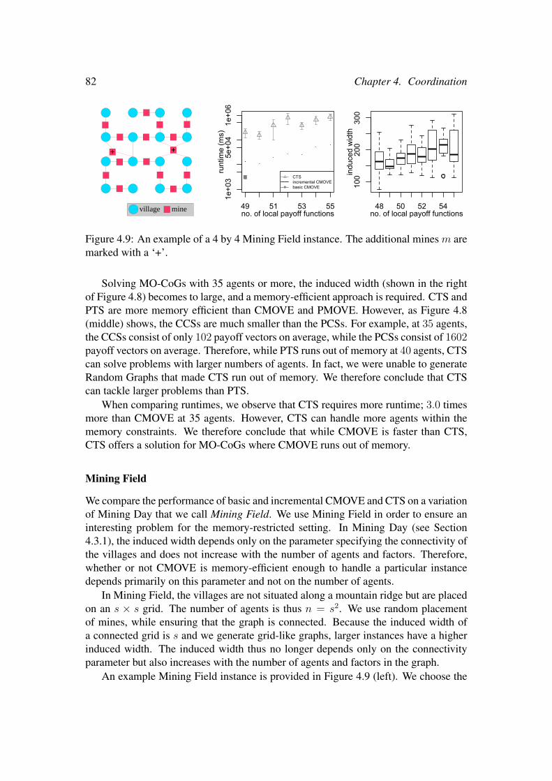
82 Chapter 4. Coordination
++
village mine 49 51 53 55
1e+03
5e+04
1e+06
no. of local payoff functionsru
ntim
e (m
s)
CTSincremental CMOVEbasic CMOVE
48 50 52 54
100
200
300
no. of local payoff functions
indu
ced
wid
th
Figure 4.9: An example of a 4 by 4 Mining Field instance. The additional mines m aremarked with a ‘+’.
Solving MO-CoGs with 35 agents or more, the induced width (shown in the rightof Figure 4.8) becomes to large, and a memory-efficient approach is required. CTS andPTS are more memory efficient than CMOVE and PMOVE. However, as Figure 4.8(middle) shows, the CCSs are much smaller than the PCSs. For example, at 35 agents,the CCSs consist of only 102 payoff vectors on average, while the PCSs consist of 1602payoff vectors on average. Therefore, while PTS runs out of memory at 40 agents, CTScan solve problems with larger numbers of agents. In fact, we were unable to generateRandom Graphs that made CTS run out of memory. We therefore conclude that CTScan tackle larger problems than PTS.
When comparing runtimes, we observe that CTS requires more runtime; 3.0 timesmore than CMOVE at 35 agents. However, CTS can handle more agents within thememory constraints. We therefore conclude that while CMOVE is faster than CTS,CTS offers a solution for MO-CoGs where CMOVE runs out of memory.
Mining Field
We compare the performance of basic and incremental CMOVE and CTS on a variationof Mining Day that we call Mining Field. We use Mining Field in order to ensure aninteresting problem for the memory-restricted setting. In Mining Day (see Section4.3.1), the induced width depends only on the parameter specifying the connectivity ofthe villages and does not increase with the number of agents and factors. Therefore,whether or not CMOVE is memory-efficient enough to handle a particular instancedepends primarily on this parameter and not on the number of agents.
In Mining Field, the villages are not situated along a mountain ridge but are placedon an s × s grid. The number of agents is thus n = s2. We use random placementof mines, while ensuring that the graph is connected. Because the induced width ofa connected grid is s and we generate grid-like graphs, larger instances have a higherinduced width. The induced width thus no longer depends only on the connectivityparameter but also increases with the number of agents and factors in the graph.
An example Mining Field instance is provided in Figure 4.9 (left). We choose the

4.3. Inner Loop CCS Methods for MO-CoGs 83
distance between adjacent villages on the grid to be unit length. On this map, we thenplace the mines (local payoff functions). We connect all agents using an arbitrary treeusing 2-agent local payoff functions (mines). In the figures, the mines that span thistree are unmarked and connected to the mines with black edges. We require s2 − 1factors to build the tree. Then we add m additional mines, by (independently) placingthem on a random point on the map inside the grid. When a mine is placed, we connectit to the villages that are within a r = 1√
2+ η radius of that mine on the map. We
chose η = 0.2. Therefore, the maximum connectivity of a factor (mine) created in thisfashion is 4. In the figure, these mines are marked with a ‘+’. The rewards per mineper worker, as well as the number of workers per village, are generated in the sameway as in Mining Day.
To compare the runtimes and memory requirements of basic and incremental CMOVEand CTS on Mining Field, we tested them on a 7 × 7 instance (49 agents) with 3 ob-jectives, and 10MB available memory. We increase the number of additional mines mfrom 2 (50 factors in total) onwards, by steps of 2. Using this setup, it was not possibleto solve any of the problem instances using PMOVE and even PTS, which ran out ofmemory for all problems.
Figure 4.9 (middle) shows that within 10 MB, basic CMOVE can solve MO-CoGsof only 49 local payoff functions or less. Contrary to our Random Graph results how-ever, incremental CMOVE can solve larger problem instances than basic CMOVE. Anexplanation for this is, is that in the Mining Field experiment, the induced width (Fig-ure 4.9 (right)) increases much more slowly than in the Random Graph experimentof Figure 4.8. We thus expect that the part that for the Mining Field experiment, thedominant factor in the memory requirements of CMOVE (Theorem 20) is the compu-tation of the cross-sums of Equation 4.6, whilst in Random Graphs the dominant partis the storage of the new VSFs. This also explains why after 55 local payoff functions,both CTS — whose main memory requirement is the computation of the cross-sums— and incremental CMOVE run out of memory. We therefore conclude that incre-mental CMOVE is more memory-efficient than basic CMOVE, and that for problemswith a low induced width CTS and incremental CMOVE use a comparable amount ofmemory.
Summarizing, we have shown that CMOVE and CTS offer different trade-offs be-tween memory and runtime. Basic CMOVE is faster than Incremental CMOVE whichis in turn faster than CTS. However, Basic CMOVE also uses most memory. Incre-mental CMOVE and CTS use less memory, and can therefore tackle larger problems.CMOVE (both basic and incremental) scales poorly in the induced width in terms ofmemory usage. CTS can solve MO-CoGs with a much higher induced width. How-ever, both the memory requirements of CTS and of CMOVE depend on the size of thecross-sums between local/intermediate CCSs. In the following Section, we proposemethods that scale much better in the size of these local/intermediate CCSs.

84 Chapter 4. Coordination
4.4 OLS for MO-CoGsIn the previous section, we showed how to create CCS methods by taking an inner loopapproach and using a single-objective search schema such as VE or TS. Furthermore,we have shown that when ample memory is available CMOVE is faster, and thereforebetter, while if memory is limited, CTS can solve MO-CoGs that CMOVE cannot. Inthis section, we create novel CCS methods using an outer loop rather than an inner loopapproach. Not only are outer loop methods easier to create than inner loop methods —as the single-objective search algorithms themselves do not have to change — and cantake any single-objective CoG solver as a subroutine, but they also have better compu-tational and space complexity bounds for small and medium numbers of objectives.
4.4.1 Variable Elimination Linear SupportRather than dealing with the multiple objectives in the inner loop of the VE searchschema, as CMOVE does, we can also employ our outer loop approach, i.e., the opti-mistic linear support we defined in Section 3.3, and employ VE as a subroutine. Werefer to the resulting algorithm as variable elimination linear support (VELS).
Because VELS uses the OLS outer loop, VELS builds the CCS incrementally, i.e.,with each iteration of its outer loop, it adds at most one new vector to a partial CCS.To find this vector, VELS selects a single w (the one that offers the maximal possibleimprovement), and passes that w to the inner loop. In the inner loop, VELS uses VE(Section 4.1.1) to solve the single-objective coordination graph (CoG) that results fromscalarizing the MO-CoG using the w selected by the outer loop. The joint action, a,that is optimal for this CoG and its payoff vector, u(a) are then added to the partialCCS. Having dealt with the multiple objectives in the outer loop of OLS, VELS thusrelies on VE to exploit the graphical structure in the inner loop.
VELS is implemented as OLS(m, SolveSODP, ε) (Algorithm 5), where,
• m is a MO-CoG, and
• SolveSODP consists of two steps: first calling VE to retrieve the optimal action,a for a scalarized instance of m, and then evaluating this action to retrieve thecorresponding payoff vector u(a).
The computational and space complexities can immediately be derived from combin-ing the computational and space complexities of OLS (Theorems 4 and 6) with thoseof VE (Theorems 11 and 12).
Corollary 6. The computational complexity of VELS
O( (|ε−CCS|+ |Wε−CCS|)(n|Amax|w + dρ+Rnw +Rheur) ),
where |Amax| is the maximal number of actions for a single agent and w is the inducedwidth, ρ is the number of factors, and Rnw and Rheur are the time it costs to runnewCornerWeights, and maxValueLP, as defined in Section 3.3.

4.4. OLS for MO-CoGs 85
Proof. This follows directly from filling in the runtime of VE, n|Amax|w, for Rso, andthe look-up and summation of ρ local payoff vectors of length d for Rpe, in Theorem4.
The overhead of OLS itself, i.e., computing new corner weights, Rnw, and calcu-lating the maximal relative improvement, Rheur, is small compared to the VE calls.Rnw + Rheur and dρ are thus negligible in practice. When comparing the runtime ofCMOVE and VELS, we observe that in the former, the runtime of VE is multiplied bythe runtime of the pruning operators (R1 andR2 in Theorem 19), while in the latter, theruntime of VE is multiplied by (|ε−CCS|+ |Wε−CCS|). Considering that |Wε−CCS| islinear in |ε−CCS| for d = 2 and d = 3, while CPrune is polynomial in the size of thelocal CCSs, we thus expect VELS to be much faster for these numbers of objectives.However, because |Wε−CCS| grows exponentially with the number of objectives (The-orem 5) we expect CMOVE to be faster than VELS for larger number of objectives.
Corollary 7. The space complexity of VELS is
O(d|ε–CCS|+ d|Wε–CCS|+ n |Amax|w).
Proof. This follows directly from filling in the memory requirements of VE, n|Amax|w,for Mso, in Theorem 4. The memory requirements for computing the payoff vector,u(a), given a are negligible.
Because OLS adds few memory requirements to that of VE, VELS is almost asmemory efficient as VE and thus considerably more memory efficient than CMOVE(Theorem 20).
4.4.2 Experiments: VELS versus CMOVEWe now empirically evaluate VELS in comparison to CMOVE. We no longer com-pare against the non-graphical method and PMOVE as these are clearly dominated byCMOVE. Where we refer to CMOVE in this section, we mean basic CMOVE, as thiswas fastest for the tested scenarios. Like before, we use both random graphs and theMining Day benchmark. All experiments in this subsection were run on a 2.4 GHzIntel Core i5 computer, with 4 GB memory.
Random Graphs
To test VELS on randomly generated MO-CoGs, we use the same MO-CoG generationprocedure as in Section 4.3.2. To determine how the scalability of exact and approxi-mate VELS compares to that of CMOVE, we tested them on random MO-CoGs withincreasing numbers of agents. The average number of factors per agent was held atρ = 1.5n and the number of objectives at d = 2. Figure 4.10 shows the results, whichare averaged over 30 MO-CoGs for each number of agents. Note that the runtimes onthe left, on the y-axis, are in log-scale but the set sizes on the right are not.

86 Chapter 4. Coordination
20 40 60 80 100
1100
10000
number of agents
runtime(ms)
CMOVEVELS (ε = 0)VELS (ε = 0.001)VELS (ε = 0.01)
20 40 60 80 100
1020
3040
number of agents
set s
ize
CCS0.001-CCS0.01-CCS
Figure 4.10: (left) The runtimes of CMOVE and VELS with different values of ε,for varying numbers of agents, n, and ρ = 1.5n factors, 2 actions per agent, and 2objectives and (right) the corresponding sizes of the ε-CCSs.
These results demonstrate that VELS is more efficient than CMOVE for two-objective random MO-CoGs. The runtime of exact VELS (ε = 0) is on average 16times less than that of CMOVE. CMOVE solves random MO-CoGs with 85 agents in74s on average, whilst exact VELS can handle 110 agents in 71s.
While this is already a large gain, we can achieve an even lower growth rate bypermitting a small ε. For 110 agents, permitting a 0.001 error margin yields a gain ofmore than an order of magnitude, reducing the runtime to 5.7s. Permitting a 0.01 errorreduces the runtime to only 1.3s. We can thus reduce the runtime of VELS by a factorof 57, while retaining 99% accuracy. Compared to CMOVE at 85 agents, VELS withε = 0.01 is 109 times faster.
These speedups can be explained by the slower growth of the ε-CCS, as we see inFigure 4.10 (right). For small numbers of agents, the size of the ε-CCS grows onlyslightly more slowly than the size of the full CCS. However, from a certain numberof agents onwards, the size of the ε-CCS grows only marginally while the size of thefull CCS keeps on growing. For ε = 0.01, the average ε-CCS grew from 2.95 payoffvectors to 5.45 payoff vectors between 5 and 20 agents, and then only marginally to5.50 at 110 agents. By contrast, the full CCS grew from 3.00 to 9.90 vectors between5 and 20 agents, but then keeps on growing to 44.50 at 110 agents. A similar pictureholds for the 0.001-CCS, which grows rapidly from 3.00 vectors at 5 to 14.75 vectorsat 50 agents, then grows slowly to 16.00 at 90 agents, and then stabilizes, to reach16.30 vectors at 120 agents. Between 90 and 120 agents, the full CCS grows from35.07 vectors to 45.40 vectors, making it almost 3 times as large as the 0.001-CCS and9 times larger than the 0.01-CCS .
To test the scalability of VELS with respect to the number of objectives, we testedit on random MO-CoGs with a constant number of agents and factors n = 25 andρ = 1.5n, but increased the number of objectives, for ε = 0 and ε = 0.1. We compare

4.4. OLS for MO-CoGs 87
2.0 3.0 4.0 5.0
1e+01
1e+05
number of objectives
runtime(ms)
CMOVEVELS (ε = 0)VELS (ε = 0.1)
2.0 3.0 4.0 5.0
520
100
500
number of objectives
set s
ize
CCS0.01-CCS0.1-CCS
Figure 4.11: (left) the runtimes of CMOVE and VELS (ε = 0 and ε = 0.1), for varyingnumbers of objectives (right) the size of the ε-CCS for varying numbers of objectives.
this to the scalability of CMOVE. We kept the number of agents (n = 25) and thenumber of local payoff functions (ρ = 37) small in order to test the limits of scalabilityin the number of objectives. The number of actions per agent was 2. Figure 4.11(left) plots the number of objectives against the runtime (in log scale). Because theCCS grows exponentially with the number of objectives, as can be seen in Figure 4.11(right), the runtime of CMOVE is also exponential in the number of objectives. VELShowever is linear in the number of corner weights, which is exponential in the sizeof the CCS, making VELS doubly exponential. Exact VELS (ε = 0) is faster thanCMOVE for d = 2 and d = 3, and for d = 4 approximate VELS with ε = 0.1 ismore than 20 times faster. However for d = 5 even approximate VELS with ε = 0.1 isslower than CMOVE.
Unlike when the number of agents grows, the size of the ε-CCS (Figure 4.11(right)) does not stabilize when the number of objectives grows, as can be seen inthe following table:
|ε–CCS| ε = 0 ε = 0.001 ε = 0.01 ε = 0.1
d = 2 10.6 7.3 5.6 3.0
d = 3 68.8 64.6 41.0 34.8
d = 4 295.1 286.1 242.6 221.7
We therefore conclude that VELS can compute a CCS faster than CMOVE for 3 ob-jectives or less, but that CMOVE scales better in the number of objectives. VELShowever, scales better in the number of agents.10 We note that these conclusions areconform expectations, because when we compare the runtimes of CMOVE and VELS
10Note that all the runtime figures in this subsection are in logscale.

88 Chapter 4. Coordination
0 100 300 500
010000
25000
number of agents
runtime(ms)
CMOVEVELS (ε = 0)VELS (ε = 1e-06)VELS (ε = 1e-05)VELS (ε = 1e-04)VELS (ε = 0.001)VELS (ε = 0.01)
1e-06 1e-04 1e-02
1e+02
5e+03
1e+05
ε
runtime(ms)
n=1000n=500n=250
Figure 4.12: (left) plot of the runtimes of CMOVE and VELS with different values ofε, for varying n (up to 500). (right) loglogplot of the runtime of VELS on 250, 500,and 1000 agent mining day instances, for varying values of ε.
(Theorem 19 and Corollary 6), CMOVE is polynomial in the size of the (local) CCSs,where VELS is merely linear in the size of the CCS and the number of corner weights(which is in turn linear in the size of the CCS for d = 2 and d = 3).
Mining Day
We now compare CMOVE and VELS on the Mining Day benchmark using the samegeneration procedure as in Section 4.3.2. We generated 30 Mining Day instances forincreasing n and averaged the runtimes (Figure 4.12 (left)). At 160 agents, CMOVEhas reached a runtime of 22s. Exact VELS (ε = 0) can compute the complete CCSfor a MO-CoG with 420 agents in the same time. This indicates that VELS greatlyoutperforms CMOVE on this structured 2-objective MO-CoG. Moreover, when weallow only 0.1% error (ε = 0.001), it takes only 1.1s to compute an ε-CCS for 420agents, a speedup of over an order of magnitude.
To measure the additional speedups obtainable by further increasing ε, and totest VELS on very large problems, we generated Mining Day instances with n ∈250, 500, 1000. We averaged over 25 instances per value of ε. On these instances,exact VELS runs in 4.2s for n = 250, 30s for n = 500 and 218s for n = 1000 onaverage. As expected, increasing ε leads to greater speedups (Figure 4.12 (right)).However, when ε is close to 0, i.e., the ε-CCS is close to the full CCS, the speedupis small. After ε has increased beyond a certain value (dependent on n), the declinebecomes steady, shown as a line in the log-log plot. If ε increases by a factor 10, theruntime decreases by about a factor 1.6.
Thus, these results show that VELS can compute an exact CCS for unprecedentednumbers of agents (1000) in well-structured problems. In addition, they show thatsmall values of ε enable large speedups, and that increasing ε leads to even biggerimprovements in scalability.

4.4. OLS for MO-CoGs 89
4.4.3 AND/OR Tree Search Linear SupportVELS is considerably more memory efficient than CMOVE. However, CTS is morememory efficient than either of them. In order to become even more memory efficientthan CTS — as well as faster for small numbers of objectives we define tree searchlinear support (TSLS).
TSLS employs OLS with TS as the single-objective solver subroutine. TSLS isequal to VELS but with VE replaced by TS. Because TSLS is an outer-loop method, itruns TS in sequence, requiring only the memory used by TS itself and the overhead ofthe outer loop, which consists only of the partial CCS (Definition 16) and the priorityqueue. Consequently, TSLS is even more memory efficient than CTS, while beingfaster for small and medium numbers of objectives.
Corollary 8. The computational complexity of TSLS is
O((|ε−CCS|+ |Wε−CCS|) (n |Amax|m +Rnw +Rheur)),
where m ≤ w log n and ε ≥ 0.
Proof. The proof is the same as that of Theorem 6 but with the time complexity of VEreplaced by that of TS (Theorem 14).
In terms of memory usage, the outer loop approach (OLS) has a large advantageover the inner loop approach, because the overhead of the outer loop consists onlyof the partial CCS (Definition 16) and the priority queue. VELS (Theorem 6) thushas much better space complexity than CMOVE (Theorem 20). TSLS has the sameadvantage over CTS as VELS over CMOVE. Therefore, TSLS has very low memoryusage, since it requires only the memory used by TS itself plus the overhead of theouter loop.
Corollary 9. The space complexity of TSLS is O(d|ε-CCS|+ d|Wε-CCS|+n)), wherem ≤ w log n and ε ≥ 0.
Proof. The proof is the same as that of Corollary 7 but with the space complexity ofVE replaced by that of TS (Theorem 13).
As mentioned in Section 4.1.2, TS is the most memory-efficient member of theclass of AND/OR tree search algorithms. Other members of this class offer differenttrade-offs between time and space complexity. It is possible to create inner loop algo-rithms and corresponding outer loop algorithms on the basis of these other algorithms.The time and space complexity analyses of these algorithms can be performed in asimilar manner to Corollaries 4 and 5 (CTS), and 8 and 9 (TSLS). The advantages ofthe outer loop methods compared to their corresponding inner loop methods howeverremain the same as for TSLS and CTS. Therefore, in this dissertation we focus on com-paring the most memory-efficient inner loop method against the most memory-efficientouter loop method.

90 Chapter 4. Coordination
4.4.4 Experiments: TSLS versus VELS and CTS
In this section, we compare TSLS to CTS, and VELS and CMOVE11. In order to testthe memory-efficiency, we limit the memory the algorithms is allowed to use, usingthe -Xmx runtime option for the JAVA Virtual Machine. All experiments use our JAVAimplementation (version 1.6 (SE)), and the corresponding MacOS X Virtual Machine.As before, we use both random graphs and the Mining Field benchmark.
To obtain the PTs for CTS and TSLS, we again use the same heuristic as CMOVEand VELS to generate an elimination order and then transform it into a PT for whichm ≤ w log n holds, using the procedure suggested by Bayardo and Miranker .
Random Graphs
First, we test our algorithms on random graphs, employing the same generation pro-cedure as in Section 4.3.2. Because connections between agents in these graphs aregenerated randomly, the induced width varies between different problems. On aver-age, the induced width increases with the number of local payoff functions, even whenthe ratio between local payoff factors and the number of agents remains constant.
In order to test the sizes of problems that the different MO-CoG solution methodscan handle within limited memory, we generate random graphs with two objectives, avarying number of agents n, and with ρ = 1.5n local payoff functions, as in previoussections. We limited the maximal available memory to 1kB and imposed a timeout of1800s.
Figure 4.13a shows that VELS can scale to more agents within the given memoryconstraints than the other non-memory efficient methods. In particular, PMOVE andCMOVE can handle only 30 and 40 agents, respectively, because, for a given inducedwidth w, they must store O(|Amax|w) local CSs. At 30 agents, the induced width(Figure 4.13c) is at most 6, while at 40 agents the induced width is at most 8. VELScan handle 65 agents, with an induced width of at most 11, because most of its memorydemands come from running VE in the inner loop, while the outer loop adds littleoverhead. VE need only store one payoff in each new local payoff function that resultsfrom an agent elimination, whereas PMOVE and CMOVE must store local coveragesets. Thus, using an outer loop approach (VELS) instead of the inner loop approach(CMOVE) already yields a significant improvement in the problem sizes that can betackled with limited memory.
However, scaling beyond 65 agents requires a memory-efficient approach. Figure4.13a also shows that, while CTS and TSLS require more runtime, they can handlemore agents within the memory constraints. In fact, we were unable to generate a MO-CoG with enough agents to cause these methods to run out of memory. TSLS is fasterthan CTS, in this case 4.2 times faster, for the same reasons that VELS is faster thanCMOVE.
11As in Section 4.4.2, where we write CMOVE, we mean basic CMOVE.

4.4. OLS for MO-CoGs 91
20 40 60 80
1e+011e+031e+05
number of agents
runt
ime
(ms)
TSLS ε = 0VELS ε = 0CTSCMOVEPMOVE
20 40 60 80
1e+011e+031e+05
number of agentsru
ntim
e (m
s)
VELS ε = 0TSLS ε = 0TSLS ε = 1e-04TSLS ε = 0.001TSLS ε = 0.01TSLS ε = 0.1
20 35 50 65 80
46
810
1214
number of agents
indu
ced
wid
th
(a) (b) (c)Figure 4.13: (a) Runtimes in ms of TSLS, VELS, CTS, CMOVE and PMOVE onrandom 2-objective MO-CoGs with varying numbers of agents n and ρ = 1.5n localpayoff factors. (b) Runtimes of approximate TSLS for varying amounts of allowederror ε, compared to (Exact) VELS, for the same problem parameters as in (a). (c) Thecorresponding induced widths of the MO-CoGs in (b).
However, speed is not the only advantage of the outer loop approach. When weallow a bit of error in scalarized value, ε, we can trade accuracy for runtime (Figure4.13b). At 65 agents, exact TSLS (ε = 0), had an average runtime of 106s, which is51 times slower than VELS. However, for ε = 0.0001, the runtime was only 70s (33times slower). For ε = 0.01 it is 11s (5.4 times slower), and for ε = 0.1 it is only6s (2.9 times slower). Furthermore, the relative increase in runtime as the number ofagents increases is less for higher ε. Thus, an approximate version of TSLS is a highlyattractive method for cases in which both memory and runtime are limited.
Mining Field
We compare the performance of VELS against TSLS on Mining Field (as defined inSection 4.3.4). We no longer consider CTS and CMOVE because these inner loopmethods have consistently higher runtime than their corresponding outer loop methods,and worse space complexity. We use Mining Field (as described in Section 4.3.4) inorder to ensure an interesting problem for the memory-restricted setting.
To compare the runtimes and memory requirements, VELS, and TSLS on MiningField, we tested them on a 7×7 instance (49 agents), with 1MB available memory. ForTSLS, we use three different values of ε: 0 (exact), 0.01 and 0.1. We use a time limitof 1.8× 10⁶s (30 minutes). We increase the number of additional mines m from 2 (50factors in total) onwards, by steps of 2.
Figure 4.14 shows the comparison between VELS and TSLS. VELS runs out ofmemory only at 16 additional factors, at an induced width of 6. Compared to therandom-graph results in Section 4.4.4, the induced widths of the problems that VELScan handle are lower in Mining Field. We suspect that this is because, on a grid-shapedproblem, the number of factors with the highest induced width that need to exist inparallel during the execution of the algorithms is higher.

92 Chapter 4. Coordination
50 54 58 62number of factors
runt
ime
(ms)
1e+01
1e+03
1e+05
VELS ε = 0TSLS ε = 0TSLS ε = 0.01TSLS ε = 0.1
50 54 58 62
23
45
6
number of factors
indu
ced
wid
thFigure 4.14: (left) Runtimes in ms of TSLS (for varying amounts of allowed error ε),VELS (ε = 0), and CMOVE on 2-objective Mining Field instances with varying num-bers of additional minesm ∈ [2..14] and a grid size of s = 7. (right) The correspondinginduced widths of the Mining Field instances.
TSLS does not run out of memory on any of the tested instances. In face, we wereunable to generate instances for which TSLS does run out of memory. However, itdoes run out of time. For ε = 0, TSLS first exceeds the time limit at m = 10 additionalmines. For ε = 0.01, this happens at m = 14. For ε = 0.1, TSLS ran out of timeat m = 16. The differences in runtime between TSLS and VELS are larger than forrandom graphs and therefore it is more difficult to compensate for the slower runtimeof TSLS by choosing a higher ε. How much slower TSLS is compared to VELS thusseems to depend on the structure of the MO-CoG.
These Mining Field results confirm the conclusion of the random-graph experi-ments that TSLS can be used to solve problem sizes beyond those that VELS can han-dle within limited memory. An approximate version of TSLS is an appealing choicefor cases in which both memory and runtime are limited.
4.4.5 Variational Optimistic Linear SupportVELS and TSLS are both exact outer loop methods, that offer different trade-offs withrespect to speed and memory usage. Furthermore, it is also possible to sacrifice accu-racy for runtime by allowing some slack ε to limit the number of calls to VE or TS.However, because VE and TS are exact single-objective solvers, this does not changethe fact that VELS and TSLS have an exponential runtime in the induced width. Toaddress this, we can instead also use an approximate single-objective solver as a sub-routine.
In this subsection we propose using variational CoG solvers, as described in Section4.1.3, as a basis for finding the CCS in a MO-CoG. As previously described, variationalmethods rely on restructuring and reparameterization rather than local summation andmaximization (like VE and TS). Therefore, it is not obvious how to apply an inner loop

4.4. OLS for MO-CoGs 93
approach. However, as an outer loop approach does not affect the inner workings of thesingle-objective solvers, it is possible to use variational methods inside OLS. This is animportant advantage for OLS, as variational methods are amongst the state-of-the-artsolvers for CoGs.
Variational solvers for CoGs are bounded approximate algorithms. Therefore, wemust use the OLS schema that allows for approximate subroutines, as described in Sec-tion 3.5. Using Algorithm 7, with a bounded-approximate variational method yieldsa new algorithm we call variational optimistic linear support (VOLS). VOLS has twoimportant advantages over VELS and TSLS. Firstly, because variational methods scalemuch better than VE and TS, VOLS achieves unprecedented scalability. In addition,since the variational method we use, which is called weighted mini-buckets (WMB) (Liuand Ihler, 2011), computes bounded approximations, VOLS does so too. Secondly, weleverage the key insight that VOLS can hot-start each call to WMB by reusing the repa-rameterizations output by WMB on earlier calls, as described in an abstract manner inSection 3.6.
In the rest of this subsection we describe how to implement reuse in OLS usingvariational methods in the VOLS algorithm. Specifically, we show how to use thereparameterizations output by a variational method as well as the lower bound forreuse in the next call to the variational solver. In Section 4.4.6 we compare VOLSempirically to CMOVE and VELS, and show that it scales much better than thesemethods at very little cost to the quality of the found solutions.
VOLS uses a variational subroutine as its instantiation of approxSolveSODP, tosolve scalarized instances of the MO-CoG. This subroutine takes a scalarized MO-CoG as input. As output, the subroutine produces a lower-bound joint action al, whichwe use to construct the approximate CCS. It also produces an upper bound u on theoptimal value, which we use to bound the quality of the final approximate CCS, andto prioritize instances in the series of single-objective problems to solve. Furthermore,the variational method manipulates the set of scalarized local payoff functions Uw tooutput a reparameterization, i.e., a set of manipulated local payoff functions U ′w forwhich all joint actions have the same (scalar) payoff:
∀a∑ue∈Uw
ue(ae) =∑ug∈U ′w
ug(ag). (4.8)
We can re-use the reparameterization, i.e., U ′w, to hot-start the reparameterizationof a new scalarized instance for a new weight vector z. Specifically, if we define thedifference graph between two scalarization weights w and z as
Uw→z = uew→z(ae) = (z−w) · ue(ae) : ue(ae) ∈ U,
then adding this difference graph to the reparameterization U ′w yields a valid reparam-eterization for z:
Uz = U ′w ∪ Uw→z.

94 Chapter 4. Coordination
When w is close to z, the magnitude of the local payoff functions in Uw→z is small,and Uz is close to U ′w. Intuitively, Uz is therefore likely to be closer to the eventualreparameterization U ′z that the variational subroutine will produce for Uz, than Uz itselfwould be, and fewer iterations of the variational method will be required to furthertighten the bounds and find U ′z. Using the difference graph Uw→z in order to hot-start the next call to a variational subroutine in OLS works for any variational single-objective CoG solver.
Using the definition of the difference graph, we can define variational optimisticlinear support (VOLS) formally. VOLS — defined in Algorithm 12 — takes a MO-CoG 〈D,A,U〉 and any variational single-objective coordination graph subroutine asinput. In this section we refer to the variational subroutine as variationalSOSolver.
Following the OLS framework, VOLS keeps a set S, that becomes an approximateCCS (line 1), a set of upper bounds on the optimal values that VOLS finds for scalar-ized instances (for individual w), Uold (line 2), and starts looking for solutions, i.e.,approximately optimal joint actions and payoffs, for the extrema of the weight simplex(line 3–4).
In order to enable the reuse of reparameterizations and lower bounds found by thevariational subroutine, VOLS keeps a set R (line 5) with tuples of weights w, andreparameterizations and joint actions that implement the lower bounds produced atthose w by variationalSOSolver in iterations of the main loop.
In the main loop (lines 6–17), VOLS iteratively pops a corner weight w off thepriority queue Q and solves the corresponding scalarized MO-CoG, Uw, as in standardOLS. However, instead of just calling the single-objective solver for Uw directly, VOLSfirst looks for the reparameterization U ′v found in earlier iterations (on line 8), for theweight closest to w. Because, the value for all joint actions remains the same whenafter reparameterizing Uv to U ′v (Equation 4.8), adding the difference graph, Uv→w
results in a graph, Uw = U ′v ∪ Uv→w, for which
∀a∑ue∈Uw
ue(ae) =∑uh∈Uw
uh(ah).
In other words, reusing the reparameterization for v on the scalarized graph for wdoes not affect the scalarized payoff, uw(a), for any a, and Uw is thus a valid repa-rameterization Uw. The aim of applying this reparameterization is for Uw to be closerto the eventual output graph U ′w of the variational solver. Our key insight is that bydoing so, the runtime of the variational single-objective solver can be drastically re-duced if the reparameterization U ′v was found at a weight v close to w. We verify thisexperimentally in Section 4.4.6.
Besides the reparameterization U ′v ∪ Uv→w, variationalSolver is also providedwith the joint action av that achieves the lower bound of the previous weight v. Thisjoint action can be reused as an initial guess for the joint action at w. If at any time dur-ing the execution of variationalSolver for U ′v∪Uv→w, the upper bound is achievedby av, the variational solver can stop. Such lower bound reuse is thus highly effec-tive when the variational single-objective solver can produce optimal solutions for the

4.4. OLS for MO-CoGs 95
Algorithm 12: VOLS(〈D,A,U〉 , variationalSOSolver)
Input: A MO-CoG1 S ← ∅; // approximate CCS of multi-objective payoff vectors u(a)2 Uold ← ∅; // set of previous w and uw, for determining optimistic estimates for new
corner weights3 Q← an empty priority queue ; // a priority queue with corner weights to search4 Add extrema of the weight simplex to Q with infinite priority;5 R← ∅ ; // set of reparameterizations, joint actions, and associated weights6 while ¬Q.isEmpty() ∧ ¬timeOut do7 w← Q.dequeue(); // retrieve a weight vector8 U ′v,av← select previous reparameterization and joint action found for the closest
weight v to w fromR;9 U ′w, al, uw ← variationalSOSolver(U ′v ∪ Uv→w) ; // a variational single
objective solver.10 R ← R∪ (w,U ′w,al) ; // store the reparameterization of the scalarized graph for
reuse11 Uold ← Uold ∪ (w, uw); // store upper bound for w, for determining the next
max. possible improv.12 if u(al) 6∈ S then13 S ← S ∪ u(al) ; // add lower bound payoff and associated action, u(al), to
the approximate CCS14 W ← compute new corner weights and max. possible improvements (w,∆w)
using Uold and S;15 Q.addAll(W );16 end17 end18 return S;
scalarized problem as it can circumvent the decoding phase of variational algorithms,which is often very computationally intensive.
The single-objective variational solver (called on line 9) produces three outputs:the new reparameterized graph U ′w, an upper bound on the optimal scalarized payoff,uw, and the approximately optimal joint action al. Note that al implies a lower boundon the optimal payoff in w, i.e., w · u(al). All of these are stored (lines 10 and 11).
If u(al) is not already in S , then it is added to it and new corner weights are identi-fied. VOLS calculates the maximum possible improvement for the new corner weightsby solving a linear program (line 14) based on the corner weights for which the vari-ational subroutine has been called, and the upper bounds found at those weights, asdescribed in Section 3.6. Finally — as is standard in OLS — the new corner weightsare added to the priority queue Q (line 15), with the maximal possible improvementsas priority. Because the maximum possible improvement to the scalarized payoff isguaranteed to be at one of the corner weights of S even when the single-objectivesubroutine is approximate (Theorem 7), VOLS terminates when Q is empty.
96 Chapter 4. Coordination
Upon termination, we can use Uold to determine the approximation quality ε, of theapproximate CCS, S using the following corollary of Corollary 2:
Corollary 10. VOLS returns S, an ε-CCS, where
ε = max(w,uw)∈Uold
(uw − u∗S(w)
).
Variational solvers for single-objective CoGs typically have no runtime guaran-tees, but are anytime and provide bounded approximations. Because OLS inherits theruntime guarantees of the single-objective solvers it employs, VOLS has no runtimeguarantees either. In our implementation we stop the single-objective solver after alimited number of iterations. However, when the lower bound becomes equal to theupper bound during an iteration of the variational single-objective solver, it can termi-nate before this maximum is reached.
Because VOLS employs reuse of the reparameterizations, the memory require-ments are are proportional to the number of weights for which a reparameterizationis stored. This storage happens on line 10, in the main loop of OLS. This hap-pens for every weight for which the variational single-objective CoG is called, i.e.,(|ε−CCS|+ |Wε−CCS|) times. The reparameterizations we use in our implementationare of (roughly) the same size as the original graphs. However, different variationalsolvers can have different reparameterization sizes.
When the memory burden of reuse becomes too big there are two possible waysto get around it: either not to do reuse, and use the variational method inside standardOLS (Algorithm 5), or to store the reparameterizations on disk rather than in memory.
To summarize, VOLS is a bounded approximate method that employs variationalCoG solvers inside OLS with reuse (Algorithm 8). These variational CoG solvershave been proven to be very effective, but have no optimality or runtime guarantees.They are however anytime, and can be stopped after a number of iterations. BecauseVOLS does not have runtime guarantees, we have to test its effectivity empirically.Furthermore, though reuse can easily be motivated intuitively — as we have done inthis subsection — it does not come with any guarantees that it is in fact faster to do so.The effectiveness of reuse must therefore be evaluated empirically as well.
4.4.6 Experiments: VOLS versus VELS
In this subsection, we compare the performance of VOLS that of VELS, as well as aversion of VOLS without reuse. We no longer compare against CTS, CMOVE, andTSLS, as these methods are slower than VELS. All experiments in this subsection useour JAVA implementation (version 1.6 (SE)). This work was carried out on the Dutchnational e-infrastructure with the support of SURF Cooperative, on a virtual machineon the HPC Cloud service, with an 2.7 GHz Intel processor. We use random graphs aswell as the Mining Day benchmark.

4.4. OLS for MO-CoGs 97
20 40 60 80 100 140
1e+02
1e+04
1e+06
number of agents
runtime(ms)
VELS (ε = 0)VELS (ε = 0.01)VOLS without reuseVOLS with reuse
20 40 60 80 100 140
0.004
0.008
0.012
number of agentsε
(as
% o
f sca
l. pa
yoff) VOLS with reuse
VOLS without reuse
20 40 60 80 100 140
0.70
0.80
0.90
1.00
number of agents
ratio
with
/with
out r
euse
runtime ratioepsilon ratio
Figure 4.15: (left) The runtime (in logscale) of VOLS versus the runtime (in logscale)of VELS as a function of the number of agents n with ρ = 1.8n and d = 3. The errorbars represent SDOM. (middle) The quality (ε) of the approximate CCSs produced byVOLS with and without reuse for the same MO-CoGs. (right) The ratio of the runtimesand ε of VOLS with and without reuse for the same MO-CoGs.
Random Graphs
In this section, we compare the performance of VELS and VOLS on randomly gen-erated MO-CoGs. For the single-objective subroutine, we use weighted mini-buckets(WMB) (Ihler et al., 2012; Liu and Ihler, 2011), with an i-bound of i = 1. i = 1is the highest degree of approximation.12 We limit the maximal number of iterationsof the single-objective subroutine at 100. The MO-CoGs are generated following theprocedure explained in Subsection 4.3.2.
We compare VELS and VOLS on random 3-objective MO-CoGs with increasingnumbers of agents n with ρ = 1.8n factors per agent. We use more objectives and ahigher ρ than we used in the previous (sub)sections, in order to create more challengingproblems, i.e., problems with a more rapidly increasing induced width and with largerCCSs. We generated 25 MO-CoGs for each number of agents and ran both algorithmson the same instances.
Figure 4.15 (left) shows that exact VELS (ε = 0) is faster than VOLS for the ran-dom graphs with up to 55 agents. However, the runtime of VELS (for any ε) increasesexponentially with the induced width, whilst that of VOLS does not. At 70 agents,VOLS is more than an order of magnitude faster than exact VELS, and at 150 agentsVOLS is still faster than exact VELS is at 70 agents.
Of course, VOLS only produces an ε-CCS, whereas exact VELS produces an exactone. However, when we measure ε using Corollary 10, we find that it is consistently1.1% of the value or less. Note that this ε needs to be determined after VOLS finishes,as VOLS does not guarantee it can reach a given ε, but instead is just limited at amaximum number of iterations of its single-objective subroutine. When we introducecomparable ε into VELS, by allowing a slack of ε of 1% (i.e., ε = 0.01), we seethat VELS remains faster than VOLS up until 75 agents. However, the runtime of
12The code was provided to us by dr. Alexander Ihler.
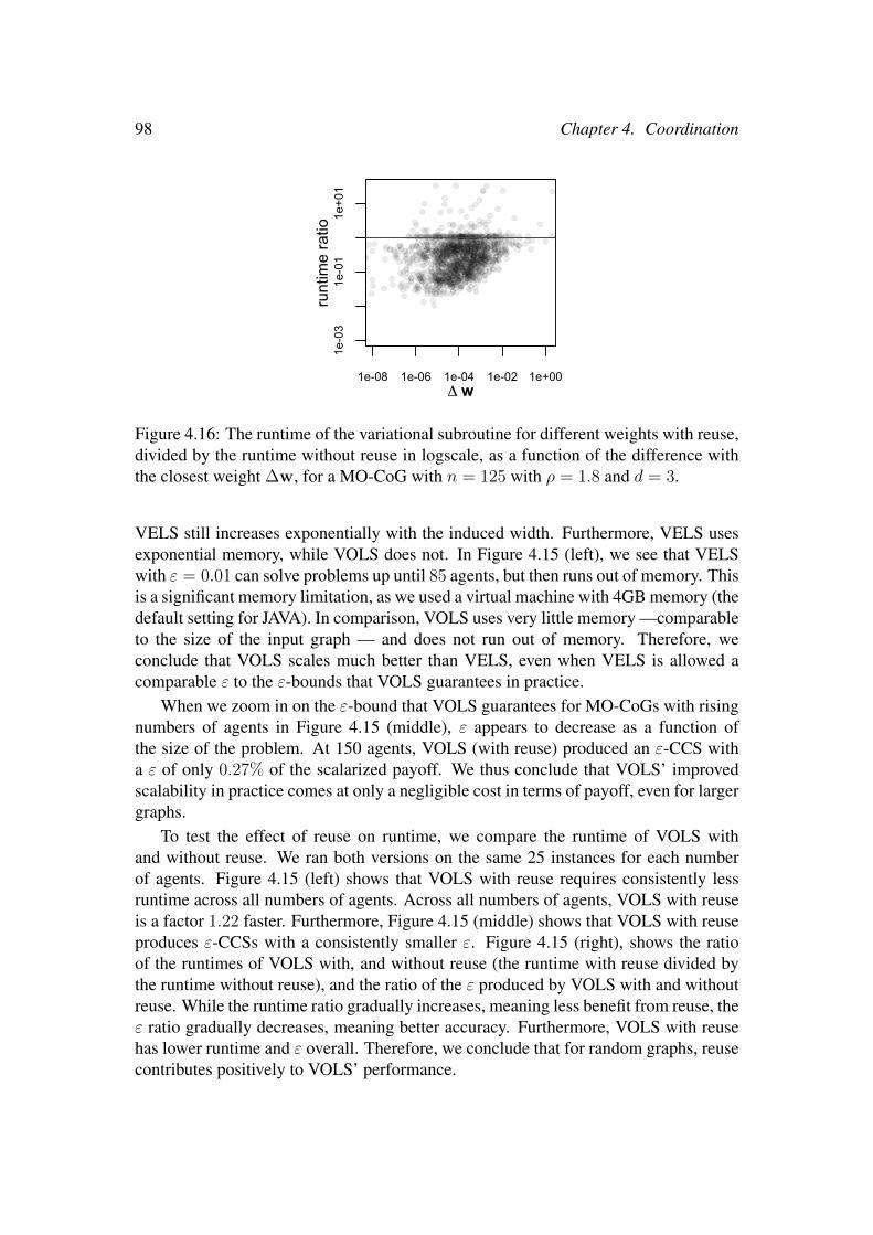
98 Chapter 4. Coordination
1e-08 1e-06 1e-04 1e-02 1e+00
1e-03
1e-01
1e+01
Δ w
runt
ime
ratio
Figure 4.16: The runtime of the variational subroutine for different weights with reuse,divided by the runtime without reuse in logscale, as a function of the difference withthe closest weight ∆w, for a MO-CoG with n = 125 with ρ = 1.8 and d = 3.
VELS still increases exponentially with the induced width. Furthermore, VELS usesexponential memory, while VOLS does not. In Figure 4.15 (left), we see that VELSwith ε = 0.01 can solve problems up until 85 agents, but then runs out of memory. Thisis a significant memory limitation, as we used a virtual machine with 4GB memory (thedefault setting for JAVA). In comparison, VOLS uses very little memory —comparableto the size of the input graph — and does not run out of memory. Therefore, weconclude that VOLS scales much better than VELS, even when VELS is allowed acomparable ε to the ε-bounds that VOLS guarantees in practice.
When we zoom in on the ε-bound that VOLS guarantees for MO-CoGs with risingnumbers of agents in Figure 4.15 (middle), ε appears to decrease as a function ofthe size of the problem. At 150 agents, VOLS (with reuse) produced an ε-CCS witha ε of only 0.27% of the scalarized payoff. We thus conclude that VOLS’ improvedscalability in practice comes at only a negligible cost in terms of payoff, even for largergraphs.
To test the effect of reuse on runtime, we compare the runtime of VOLS withand without reuse. We ran both versions on the same 25 instances for each numberof agents. Figure 4.15 (left) shows that VOLS with reuse requires consistently lessruntime across all numbers of agents. Across all numbers of agents, VOLS with reuseis a factor 1.22 faster. Furthermore, Figure 4.15 (middle) shows that VOLS with reuseproduces ε-CCSs with a consistently smaller ε. Figure 4.15 (right), shows the ratioof the runtimes of VOLS with, and without reuse (the runtime with reuse divided bythe runtime without reuse), and the ratio of the ε produced by VOLS with and withoutreuse. While the runtime ratio gradually increases, meaning less benefit from reuse, theε ratio gradually decreases, meaning better accuracy. Furthermore, VOLS with reusehas lower runtime and ε overall. Therefore, we conclude that for random graphs, reusecontributes positively to VOLS’ performance.

4.4. OLS for MO-CoGs 99
100 300 500
010000
25000
number of agents
runtime(ms)
VELS (ε = 0)VOLS with reuseVOLS without reuse
Figure 4.17: Plot of the runtimes of VOLS (with and without reuse) and VELS (ε = 0)with different values of ε, for varying n.
In order to test our hypothesis that reuse is more effective when the reparameteriza-tion reused for a weight w was found at a weight z closer to w, we tested the effect ofreuse on the runtime of the single-objective subroutine inside VOLS. For this purpose,we used a single MO-CoG with d = 3, n = 125 and ρ = 1.8n. For each weight win the sequence, we executed the variational subroutine with and without reuse. Theaverage total runtime with reuse was 0.10s while it was 0.16s without reuse. Fig-ure 4.16 shows the ratio between the runtime with and without reuse as a function of∆w = |z −w|, i.e., the Euclidean distance between the current weight on the weighton which the reused reparameterization is based. This figure shows that the runtimeis positively correlated with ∆w. However, there are also a lot of weights for whichreuse has little or no effect, and even outliers for which reuse has a negative effect onthe runtime. These outliers contribute disproportionally to the average runtime: al-though they make up only 5% the weights, they are responsible for 48% of the totalruntime of VOLS with reuse. For comparison, the first 5% of the calls, i.e., those withthe 5% largest ∆w, account for only 9% of the runtime. We therefore conclude thatour hypothesis seems correct on average, but that a small ∆w is not a guarantee for alow runtime.
Mining Day
In order to compare VOLS and VELS on a highly structured problem, with limitedinduced width, we use the Mining Day benchmark. We use the same generation proce-dure as in Section 4.3.2, with 2-5 workers per village and a connectivity of 2-4 minesper village. We generated 25 Mining Day instances for increasing n and averaged theruntimes.
Because the induced width of this problem is limited by the maximum numberof mines per village, the induced width does not increase with the number of agent.

100 Chapter 4. Coordination
Furthermore, because we use a maximum connectivity of 4, the induced width is alsolow.
In Figure 4.17, we see that exact VELS (ε = 0) outperforms VOLS — both withand without reuse. At 220 — at which point we stopped running VOLS — VOLS was147 (with reuse) respectively 42 (without reuse) times slower than VELS. We thereforeconclude that in problems with a low induced width, VOLS does not scale better thanVELS in the number of agents.
When we inspect how VOLS with reuse compared to VOLS without reuse, we seethat VOLS without reuse seems to perform better in terms of runtime than VOLS withreuse. However, the ε of VOLS with reuse is better than without reuse: the maximalε for VOLS with reuse was 1.5 × 10⁻⁶ and has an average of 1.5 × 10⁻⁹, against amaximum of 1.0×10⁻³ and an average of 8.7×10⁻⁶ for VOLS. We therefore concludethat for Mining Day, reuse makes VOLS slower rather than faster, although it slightlyimproves the ε.
4.5 ConclusionIn this chapter, we proposed several novel algorithms for computing a CCS for MO-CoGs. These new methods either follow an inner loop approach (CMOVE and CTS),or an outer loop approach based on OLS (VELS, TSLS, and VOLS).
When we compare our inner loop methods to corresponding inner loop methodsthat compute the PCS, we find that our CCS methods scale much better in the sizeof the MO-CoG as well as in the number of objectives. Therefore, we conclude thatcomputing a CCS should be preferred over computing a PCS whenever possible. Aswe have argued in Chapter 2, the CCS applies to both the case when the scalarizationfunction is linear and to the case when stochastic policies are allowed.
When we compare inner loop methods to corresponding OLS-based methods, i.e.,methods that use the same single-objective search schema as a basis, we find that innerloop methods scale better in the number of objectives, while OLS-based methods scalebetter in the number of agents. We argue that the latter is usually more important inpractice.
When compared our exact methods, i.e., CMOVE, CTS, VELS and TSLS. CMOVEand VELS are fastest. For 2 and 3 objectives, VELS is faster than CMOVE. VELS alsoscales better in the number of agents. However, CMOVE scales better in the number ofobjectives. Both CMOVE and VELS use an exponential (in the induced width) amountof runtime, while CTS and TSLS use an amount of memory independent of the inducedwidth. Between CTS and TSLS, TSLS is most memory efficient.
When exact CCSs are not required, VELS and TSLS (but not CMOVE and CTS)can produce ε-CCSs for any pre-specified ε. Doing so can result in a decrease inruntime of orders of magnitude, even for small ε.
When it is not necessary to pre-specify a given ε, VOLS outperforms the othermethods in terms of runtime and memory use. As we have seen from our random

4.5. Conclusion 101
graph experiments, VELS and TSLS use an amount of runtime and memory that isexponential in the induced width, while VOLS does not. However, when the inducedwidth is limited (as in Mining Day) VELS is typically faster than VOLS, even whenVELS solves the MO-CoG exactly (ε = 0).
To summarize, we have proposed five different CCS algorithms for MO-CoGs.These methods are typically much faster than corresponding PCS methods. Comparedto each other, our methods provide different trade-offs between runtime, memory, andoutput quality (ε).


Chapter 5Sequential Decision-Making
In the previous chapter, we have considered problems in which a single (joint) actionis performed in order to obtain a reward. However, many decision problems consistof a sequence of decisions. This sequence of decisions typically takes place in anenvironment that is affected by these decisions. Therefore, the agents do not only haveto consider their immediate reward, but also the reward they will be able obtain later,by changing the state of the environment to a more favorable one.
In this dissertation, we consider two multi-objective sequential single-agent deci-sion-theoretic models. The first model is fully observable and extends the single-objective Markov decision process (MDP) (Bellman, 1957b; Puterman, 1994; Suttonand Barto, 1998; Wiering and Van Otterlo, 2012). The second is partially observ-able and extends the partially observable Markov decision process (POMDP) (Cas-sandra, 1998; Kaelbling et al., 1998; Spaan, 2012). The single-objective version ofthese models are widely used and applied in areas such as: communication networks(Altman, 2002), planning and scheduling (Scharpff et al., 2013), games (Szita, 2012)and robotics (Kober and Peters, 2012). The multi-objective models have been gain-ing traction relatively recently. There is a significant body of work on multi-objectiveMarkov decision problems (MOMDPs) (Roijers et al., 2013a), and recently, there havebeen several papers on multi-objective partially observable Markov decision problems(MOPOMDPs) (Soh and Demiris, 2011a,b; Roijers et al., 2015c; Wray and Zilberstein,2015).
In this chapter we propose new methods for MOMDPs and MOPOMDPs based onOLS. We focus on challenging instances of these models, and show that state-of-the-art methods for single-objective planning can be effectively employed as subroutinesin OLS in order to create multi-objective methods, with relatively little effort. This is amajor advantage, for it implies that if the state-of-the-art for single-objective methodsimproves, then — via OLS — so does the state-of-the-art in multi-objective methods.
For MOMDPs, we focus on finite-horizon problems with a very large state-space.Specifically, we employ the multi-objective version of the maintenance planning prob-lem (MPP) (Scharpff et al., 2013; Roijers et al., 2014a; Scharpff et al., 2015, 2016)
103

104 Chapter 5. Sequential Decision-Making
as an illustrative example problem. The main challenge in both the single- and multi-objective MPP is the size of the state and action spaces. For this problem, a highlyproblem-specific solution method exists which makes use of a SPUDD (Hoey et al.,1999) encoding. An inner loop method that uses such a problem-specific encoding(and SPUDD itself) as a base for a multi-objective method, takes a lot of time to cre-ate. Furthermore, the construction of the inner loop method has to be redone for everydifferent problem that requires such a problem-specific solution method or when astate-of-the-art method for the single-objective version of a problem is invented. InSection 5.2, we show that we can create effective multi-objective methods based onOLS that do not have these disadvantages. We illustrate this by exchanging SPUDDand its encoding by the CoRe algorithm which we proposed recently (Scharpff et al.,2016). Furthermore, we show that by using an approximate solver, i.e., UCT∗ insteadof an exact solver, ε-CCSs can be found in a fraction of the runtime it takes to computean exact CCS.
For POMDPs, we focus on infinite-horizon problems. Creating planning meth-ods for single-objective POMDPs is an active field of research (Kurniawati et al.,2008; Pineau et al., 2006; Poupart et al., 2011), and as such, is regarded a hard andopen problem. Therefore, extending the POMDP model to the multi-objective set-ting, i.e., multi-objective POMDPs (MOPOMDPs), results in a very computationallychallenging problem. Maybe this is one of the reasons why only a few papers aboutMOPOMDPs exist. In Section 5.3, we propose the first planning method for multi-objective POMDPs that computes a CCS and scales reasonably well. In order to doso, we use point-based planning methods (Shani et al., 2013), and specifically Perseus(Spaan and Vlassis, 2011), as a single-objective subroutine. We show that it is highlybeneficial to employ reuse (Section 3.6) of the value functions found in previous OLSiterations. In order to enable this reuse — and to avoid separate policy evaluations,which can be expensive in POMDPs — we show how to create OLS-compliant ver-sions of point-based planning methods, that use a multi-objective representation of thevalue function.
The rest of this chapter is structured as follows. We introduce MDPs, MOMDPs,POMDPs and MOPOMDPs in Section 5.1. In Section 5.2, we show how we can createefficient methods for large MOMDPs, using the MPP as an illustrating problem. InSection 5.3 we propose OLS with Alpha Reuse (OLSAR), which is our main contribu-tion for MOPOMDPs. We conclude in Section 5.4, with a summary of our results.
5.1 Background
In this section we provide the requisite background on the MOMDP and MOPOMDPmodels. However, we first describe their single-objective counterparts.

5.1. Background 105
5.1.1 Markov decision processes
First, we describe the fully observable setting.
Definition 32. A (single-objective) Markov decision process (MDP) (Wiering andVan Otterlo, 2012) is a tuple 〈S,A, T, R〉 where,
• S is the state space, i.e., the set of possible states the environment can be in,
• A is the action space, i.e., the set of actions the agent can take,
• T : S×A×S → [0, 1] is the transition function, giving the probability of a nextstate given an action and a current state,
• R : S × A × S → R is the reward function, specifying the expected immediateexpected scalar reward corresponding to a transition.
At each timestep t the agent observes the current state of the environment s ∈ S .When the agent takes an action a ∈ A the environment transitions to a new state s′.
The state in an MDP is Markovian, i.e., the current state s of the environmentand the current action of the agent a are a sufficient statistic for predicting the nexttransition probabilities T (s′|s, a) and the associated expected immediate reward. Theagent’s history, i.e., the states and actions that led to the current state, do not provideadditional information in that respect.
The agent’s goal in an MDP is to find a policy that maximizes the expected sum offuture rewards. Informally, a policy is a set of decision rules that for each point in timeand state of the MDP, prescribes how to choose an action to perform. The expectedsum of future rewards given a policy, π, is called the value of π, V π. In a finite-horizonsetting there is a limited number of timesteps, h, and the sum is typically undiscounted:
V π = E[h∑t=0
R(st, at, st+1)|π, µ0],
where µ0 is the distribution over initial states s0. In a discounted infinite-horizon set-ting, the number of timesteps is not limited, but there is a discount factor, 0 ≤ γ ≤ 1,that specifies the relative importance of future rewards with respect to immediate re-wards:
V π = E[∞∑t=0
γtR(st, at, st+1)|π, µ0].
There are different choices for what to condition a policy on. We refer to the set ofall possible policies for an MDP as Π. A stationary policy is one that conditions theactions only on the current state, S×A → [0, 1], i.e., for each state there is a probabilitydistribution over actions. We refer to the set of all possible stationary policies as ΠS .

106 Chapter 5. Sequential Decision-Making
Non-stationary policies can besides the state also condition on the timestep t.1 Anotherspecial type of policy is a deterministic policy. A deterministic policy only assigns 0or 1 probabilities to actions for each value of what it conditions on. A deterministicstationary policy thus specifies a single action in each state S → A. We refer to the setof all possible deterministic policies as ΠD, and the set of all deterministic stationarypolicies as ΠDS .
For infinite horizon MDPs we can restrict the search to deterministic stationarypolicies in order to find an optimal policy. For finite horizon MDPs we can restrictrestrict the search to deterministic non-stationary policies.
Theorem 21. (Boutilier et al., 1999; Howard, 1960) For any infinite-horizon single-objective MDP, there exists a deterministic stationary policy, π∗ ∈ ΠDS that is optimal.
Theorem 22. (Boutilier et al., 1999) For any finite-horizon single-objective MDP,there exists a deterministic policy π∗ ∈ ΠD that is optimal.
The existence of an optimal deterministic policy drastically reduces the size of thespace of policies that need to be considered. In the case of finite-horizon MDPs thereare |ΠD| = |A|h|S| policies to consider, and for infinite-horizon MDPs even |ΠDS| =|A||S|, while there would be infinitely many if we consider stochastic policies as well.Optimal policies in MDPs can be found efficiently using e.g., dynamic programmingtechniques (Bellman, 1957a) or linear programming (Manne, 1960).
Definition 33. A multi-objective Markov decision process (MOMDP) (Roijers et al.,2013a) is a tuple 〈S,A, T, R〉 where,
• S, A, and T are the same as in an MDP,
• R : S ×A× S → Rd is the reward function, specifying the expected immediatevector-valued reward corresponding to a transition.
When only deterministic policies are allowed and the scalarization function, f , isnonlinear, non-stationary policies can be better than the best stationary ones. There-fore, unlike in single-objective MDPs, it is not always the case that we only need toconsider deterministic stationary policies.
Theorem 23. (White, 1982) In infinite-horizon MOMDPs, deterministic non-stationarypolicies can Pareto-dominate deterministic stationary policies that are undominated byother deterministic stationary policies.
To see why, consider the following infinite-horizon MOMDP with discount factorγ, which was adapted from an example by White (1982): there is only one state, s andthree actions a1, a2, and a3, which yield rewards (3, 0), (0, 3), and (1, 1), respectively.The transitions (for all actions) from state s all lead back to the same state. If we
1Note that there are also other options to condition on, e.g., the entire history of states and actions.For sake of brevity we not consider these here.

5.1. Background 107
0 10 30 50
020
4060
V0
V1 Vπns
Vπ3
Vπ1
V π2γ=0.95
Figure 5.1: The policy values of π1, π2, π3, and πns for the example MOMDP byWhite (1982), for γ = 0.95. The blue line indicates the possible values for all possiblemixture policies that use π1 and π2 as base policies.
allow only deterministic stationary policies, then there are only three possible policiesπ1, π2, π3, each corresponding to always taking one of the actions, all of which arePareto optimal. These policies have the following values: Vπ1 = (3/(1 − γ), 0),Vπ2 = (0, 3/(1−γ)), and Vπ3 = (1/(1−γ), 1/(1−γ)). However, if we now considerthe set of possibly non-stationary policies, we can construct a policy πns that alternatesbetween a1 and a2, starting with a1, whose value is Vπns = (3/(1− γ2), 3γ/(1− γ2)).Consequently, this policy Pareto-dominates π3, πns P π3 when γ ≥ 0.5 (Figure5.1) and thus we cannot restrict our attention to stationary policies. Note that similarexamples can be constructed for the finite-horizon setting.
For linear f however, we can restrict our attention to only deterministic stationarypolicies (Roijers et al., 2013a):
Theorem 24. For an infinite-horizon MOMDP m, any CCS(ΠDS) of deterministicstationary policies is also a CCS(Π) for stochastic non-stationary policies.
Proof. This proof is similar to that of Theorem 1 and Theorem 3. If f is linear, wecan translate the MOMDP to a single-objective MDP, for each possible w. This isdone by treating the inner product of the reward vector and w as the new rewards, andleaving the rest of the problem as is. Since the inner product distributes over addition,the scalarized returns remain additive. Thus, for every w there exists a translation toa single-objective MDP, for which an optimal deterministic and stationary policy mustexist, due to Theorem 21. Consequently, when the optimal deterministic stationarypolicy for w is πw, there cannot exist a non-stationary and/or stochastic policy, π′, suchthat w ·Vπ′ > w ·Vπw . Because this holds for every possible w, a CCS with respectto all deterministic stationary policies is also a CCS for all stochastic non-stationarypolicies.

108 Chapter 5. Sequential Decision-Making
Any deterministic stationary CCS is thus sufficient for solving infinite-horizonMOMDPs with linear f , even when stochastic and non-stationary policies are allowed.For finite-horizon MOMDPs a similar theorem holds but for deterministic (possiblynon-stationary) policies only:
Theorem 25. For a finite-horizon MOMDPm, anyCCS(ΠD) of deterministic policiesis also a CCS(Π) for stochastic policies.
Proof. The proof is identical to that of Theorem 24.
In the proof of Theorem 24 we show than an MOMDP can be scalarized with a lin-ear weight w, resulting in an MDP. Because this fulfills the conditions of Assumption1), we can use a deterministic CCS as a compact representation of a PCS for stochasticpolicies (Corollary 1). In Figure 5.1 for example, the values in the PCS of stochasticpolicies for the abovementioned MOMDP example by White (1982) are indicated bythe blue line; these values can all be attained by mixing π1 and π2.
5.1.2 Partially Observable Markov Decision ProblemsSo far we have assumed that the state of the environment can be observed by the agent.However, in many planning problems this is not the case. For example, imagine arobot that has only a front camera as sensor input and needs to go to a given location inan office building. When driving around, many locations in such a building may lookidentical (especially in the hallways). Therefore the agent controlling the robot hasto rely on the memory of its previous observations to disambiguate the state as muchas possible. The partially observable Markov decision process (POMDP) (Kaelblinget al., 1998) is a decision-theoretic model that incorporates partial observability into asingle-agent sequential decision problem.
Definition 34. A POMDP is a tuple 〈S,A, T, R,Ω, O〉 where,
• S, A, T , and R are the same as in an MDP,
• Ω, is the set of possible observations, and
• O is the observation function, giving the probability of each observation givenan action and the resulting state, i.e., O(o|a, s′) is the probability of observingo ∈ Ω when taking action a resulting in state s′ (regardless of the state in whichaction a was taken). It is thus a mapping: A× S × Ω→ [0, 1].
Because the agent cannot observe the entire state, the history of previous observa-tions yields information about the present state that is not contained in the latest obser-vation. In other words, the observations the agent receives are not Markovian, and onlyconditioning on the last observation could lead to loss of optimality. This makes theplanning problem in POMDPs much harder than in an MDP. In fact, infinite-horizonPOMDPs are in general undecidable (Madani et al., 2003). However, there is some

5.1. Background 109
leverage that can be used for planning. Specifically, it turns out that the belief state ofan agent is a sufficient statistic for the (action-observation) history of an agent, and canbe used as a Markovian state signal.
Definition 35. The belief state b(s), specifies for each state s ∈ S the probability ofbeing in that state s.
In a POMDP, an agent can maintain such a belief b(s) (Astrom, 1965). We call thebelief of an agent at timestep 0, b0(s). The agent updates its belief when it takes anaction a, makes an observation o, according to the following update rule:
bt+1(s′) =O(o|s′, a)
P (o|bt, a)
∑s∈S
T (s′|s, a)bt(s),
where,Pb(o|bt, a) =
∑s′∈S
O(o|s′, a)∑s∈S
T (s′|s, a)bt(s).
We can use the belief updates to specify a transition function for belief-states, Tb(b′|a, b).Specifically, in a given belief bt, the next belief bt+1 only depends on the action aand the observation o, and the probability of an observation is P (o|bt, a). Further-more, we can also specify a reward function Rb(b, a) =
∑s∈S b(s)R(s, a), where
R(s, a) =∑
s′∈S R(s, a, s′)T (s′|s, a). Together, the belief-state, Rb, and Tb can beused to specify a belief-MDP.
Theorem 26. (Spaan, 2012) For each POMDP 〈S,A, T, R,Ω, O〉, there is an equiv-alent belief-MDP 〈Sb = ∆S,A, Tb, Rb〉, where ∆S is the belief simplex, i.e., all validprobability distributions over S, A is the same set of actions as in the POMDP, andTb and Rb are as specified above. An optimal policy for this belief-MDP is an optimalpolicy for the POMDP, and the optimal value function for the belief-MDP is equal tothe optimal value function for the POMDP.
Corollary 11. For any discounted infinite-horizon (single-objective) POMDP, thereexists an optimal deterministic stationary policy conditioned on the belief. For anyfinite-horizon (single-objective) POMDP, there exists an optimal deterministic policyconditioned on the belief.
Proof. This follows directly from Theorems 21, 22, and 26.
The value function for a single-objective POMDP, V (b), can thus be defined interms of the belief state. The value function can be represented by a set V of α-vectors.Each vector α (of length |S|) gives a value for each state s. The value of a belief bgiven V is:
V (b) = maxα∈V
b · α. (5.1)
Equation 5.1 implies the following observation:

110 Chapter 5. Sequential Decision-Making
Observation 3. (Sondik, 1971) The value function of a POMDP is a piecewise-linearand convex (PWLC) function in b.
Each α-vector is associated with an action. Therefore, a set of α-vectors V alsoprovides a policy πV that for each belief takes the maximizing action in Equation 5.1.
Because infinite-horizon POMDPs are in general undecidable, the exact optimalvalue function and accompanying α-vectors cannot be found exactly within finite time.An ε-approximate value function can in principle be computed using techniques likevalue iteration (VI) (Monahan, 1982) and incremental pruning (Cassandra et al., 1997).Unfortunately, these methods scale poorly in the number of states. However, point-based methods (Shani et al., 2013), which approximate the value function for the entirebelief simplex by iteratively computing the best α-vector only for a set B of sampledbeliefs, scale much better. We explain how this works in Section 5.3.1.
Definition 36. An MOPOMDP is a tuple 〈S,A, T,R,Ω, O〉 where,
• S, A, T , Ω, and O are the same as in a POMDP,
• R : S ×A× S → Rd is the reward function, specifying the expected immediatevector-valued reward corresponding to a transition.
For MOPOMDPs, we observe that because of the equivalence between POMDPsand belief MDPs (Theorem 26 and Corollary 11), Theorem 24 also extends to POMDPs,i.e.,
Corollary 12. For an MOPOMDP, any CCS of deterministic stationary policies —with respect to belief-state — is also a CCS for stochastic non-stationary policies.
Furthermore, because MOPOMDPs can be scalarized to a POMDP equivalently toscalarizing a MOMDP, i.e., by taking the inner product of a weight vector w and thereward function R as the scalarized reward function, and leaving the rest of the problemintact, the CCS of deterministic policies can be used as a compact representation of thePCS of stochastic policies (Corollary 1).
The only current method available for computing a CCS for a MOPOMDP is basedon an old method for MOMDPs. White and Kim (1980) proposed a method to trans-late a multi-objective MDP into a POMDP, which can also be applied to a MOPOMDPand yields a single-objective POMDP. Intuitively, this translation assumes there is onlyone “true” objective. Since the agent does not know which objective is the true one,this yields a single-objective POMDP whose state is a tuple 〈s, i〉 where s is the orig-inal MOPOMDP state and i ∈ 1 . . . d indicates the true objective. The resultingPOMDP’s state space is of size |S|d. The observations provide information about sbut not about i. The resulting POMDP can be solved with standard methods but onlythose that do not require an initial belief, as such a belief would fix not only a dis-tribution over s but also over i, yielding a policy optimal only for a given w. Sincethis precludes the effective usage of solvers like point-based methods, it is a severelimitation.

5.2. OLS for Large Finite-Horizon MOMDPs 111
For PCSs, no theorem like Corollary 12 exists. In fact, the only current researchwe are aware of that aims to find a PCS for a given MOPOMDP is by Soh and Demiris(2011a,b) who use evolutionary methods to approximate the PCS. However, evolution-ary methods are heuristic algorithms that provide no guarantees regarding the qualityof the approximation. Furthermore, as we discuss in Section 2.3, finding a PCS isoften not necessary. In Section 5.3, we show how to employ the class of point-basedplanning algorithms (Shani et al., 2013) — to which many state-of-the-art planningmethods for POMDPs belong — as subroutines in OLS, to create planning methodsfor MOPOMDPs and how these methods can provide bounds on the quality of theapproximation.
5.2 OLS for Large Finite-Horizon MOMDPsIn this section, we show how to tackle challenging real-world MOMDPs using OLS.The problem we use to illustrate this is called the maintenance planning problem(MPP) (Scharpff et al., 2013; Roijers et al., 2014a; Scharpff et al., 2015, 2016). Wefirst introduce the MPP and explain why it is a computationally hard problem. Thenwe briefly discuss the existing single-objective methods for the MPP, explain the intu-ition behind how these are able to solve the MPP efficiently, and how to use them assubroutines inside OLS. Finally, we compare the different subroutines in combinationwith OLS on instances of the MPP.
5.2.1 The Maintenance Planning ProblemThe maintenance planning problem (MPP) (Scharpff et al., 2013; Roijers et al., 2014a;Scharpff et al., 2015, 2016) is a task-based planning problem in which a governmentneeds to have road maintenance tasks performed. The government wants to minimizemaintenance costs that it will ultimately have to pay (objective 1) while minimizingthe hindrance of these maintenance tasks to traffic (objective 2). In order to do so, theyplace fines on causing traffic delay.
In order achieve their objectives, the local government uses a public tender to at-tract a group of contractors. Each contractor bids on a set of predetermined main-tenance tasks. The tender is based on a dynamic-VCG mechanism (Bergemann andValimaki, 2006; Cavallo, 2008). In this mechanism, the rewards for a contractor are agiven weighted sum (i.e., a linear scalarization with a given weight w) of the paymentit receives from the government minus the costs of the maintenance tasks and the fines.Because of the mechanism, the optimal strategy for each contractor is to be truthfulabout the costs, and to cooperate in planning a policy for performing the maintenancetasks. In other words, because of the mechanism, the problem becomes a fully coop-erative multi-agent MDP. Therefore, we will refer to the contractors as the agents, andto the multi-agent MDP as the single-objective MPP. A condition for being able to usethe mechanism however, is that the optimal policy can be computed.

112 Chapter 5. Sequential Decision-Making
The government has estimates of the costs for each contractor based on previoustenders. However, in previous tenders, there was too much traffic delay. Therefore,the government wants to incentivize performing a policy that results in less hindrancefor traffic by adding to the fines on traffic delay, i.e., they want to investigate the effecton the value of the optimal policies (i.e., the total costs and the total traffic delay) bychanging w. This can be modelled as finding the CCS a multi-objective multi-agentMDP. After finding the CCS, the local government can select a w for which the optimalpolicy of the contractors corresponds to the value vector the government selected fromthe CCS. We refer to this multi-objective multi-agent MDP as the multi-objective MPP.
It is important that the CCS can be computed exactly. Otherwise, the dynamic-VCG mechanism no longer guarantees that rational agents are truthful (Scharpff et al.,2013), and we can no longer model the MPP as a multi-objective MMDP. Therefore,we focus on using exact planning methods. However, approximate methods could stillbe used by the local government to get a global idea about the values in the CCS.
In the multi-objective MPP, each task has a minimal completion time. Dependingon conditions that become known at the moment the task is started, a task may delaywith a given amount of time. The probability of delay is known.
The hindrance for traffic depends on which tasks are performed concurrently. Forinstance, concurrent maintenance in a busy area causes more hindrance than whenmaintenance tasks are performed sequentially.
The maintenance tasks for a given agent i are a fixed predetermined set. For eachtask, a, there are
• a number of consecutive time steps required to complete the task, d ∈ Z+,
• the probability that a task will delay, p ∈ [0, 1],
• the additional duration if the task is delayed, d ∈ Z+, and
• a cost function, c(a, t), that captures the cost of maintenance (e.g., personnel,materials, etc.) per time step t ∈ [1, . . . , h].
The reward for executing a maintenance task is a (time-independent) payment, minusthese costs. This is the first objective in the multi-objective MPP. Note that the costsmay differ for each time step (e.g., it may be more expensive to perform a task at nightor during holiday periods). The total cost of the execution of a task is the sum ofthe costs for each time step the task is being executed including delays. Agents arerestricted to executing a single task per time step and they can only plan activities ifthey are guaranteed to finish them within the plan horizon. Because the payments areindependent of time, while the costs are dependent of time, the agents want to scheduletheir tasks at the cheapest time-slots. However, there is also an incentive for agents tocooperate and not schedule too many tasks in parallel, because of the fines that areincurred by traffic hindrance.
The hindrance caused by maintenance is given by the function `(At, t), expressedin traffic time lost (TTL). In this function, At is used to denote any combination of

5.2. OLS for Large Finite-Horizon MOMDPs 113
maintenance tasks performed at time t, by one or more agents. This function is typi-cally based on traffic simulations, but can also be computed using heuristic rules. TTLis the second objective in the multi-objective MPP.
In the multi-objective MPP, the state is defined as the activities yet to be performed(for all agents together), the time left to perform them, and the availability of the indi-vidual agents (as they may currently be executing a task). The possible actions for asingle agent are starting a task that has not been performed yet (if not busy), continuea task (if busy), or do nothing (if not busy). For more details on the MPP please referto (Scharpff et al., 2013).
The main challenge in the MPP is that both the size of the state space and the sizeof the action space are exponential in the number of agents (Boutilier, 1996). Further-more, contrary to decentralized models (Becker et al., 2003; Nair et al., 2005; Witwickiand Durfee, 2010), the policy for each agent needs to condition on the entire (expo-nentially sized) state space in order to be optimal, as agents can predict the actions ofother agents better based on the full state than based on only their own local state (as indecentralized models) (Scharpff et al., 2016). Therefore, planning needs to take placein a centralized manner, i.e., as if a single agent controls all others. It is, in general, notpossible to tell how much value would be lost if a decentralized approach were takenas an approximation. Fortunately though, this does not mean that is impossible to ex-ploit the structure of the MPP. It is however necessary to formulate tailored solutionmethods to the specific properties of the MPP.
5.2.2 Solving MPP instancesIn the single-objective version of the MPP, a monetary value is assigned to each hourof traffic time lost (TTL), thereby linearly scalarizing the problem. For this single-objective problem, we discuss three solution methods as proposed by Scharpff et al.(2013), Roijers et al. (2014a) and (Scharpff et al., 2016). We later use these methodsas the single-objective subroutine in OLS, in order to solve the multi-objective MPP.The single-objective methods are
• SPUDD + compact encoding — The stochastic planning using decision dia-grams (SPUDD) algorithm (Hoey et al., 1999), is a value iteration algorithm thatemploys algebraic decision diagrams (ADDs) to represent value functions andpolicies. ADDs are compact representations that use state features — such aswhether a task has already been performed or not in the MPP — to describethe value function. By doing so, many states are (implicitly) grouped together,leading to compact representations of the value function (or policy). SPUDDimplements dynamic programming (Bellman, 1957a) via manipulation of theseADDs. Therefore, SPUDD can handle large state spaces well, as long as thesestate spaces are structured.
However, the MPP has a large action space as well as a large state space. There-fore, Scharpff et al. (2013) propose an encoding of the single-objective MDP
114 Chapter 5. Sequential Decision-Making
that reduces the size of the action space (at the cost of slightly increasing thesize of the state space). In this encoding, one time step is split up in one timestep per agent. At each such a “sub time step” an agent commits to carrying outan action from its own available actions (i.e., tasks to perform, continue or donothing), and augmenting this commitment to the state. In this manner, an MDPthat SPUDD can handle is created.
SPUDD is an exact single-objective planning method, and can thus be used inconjunction with the dynamic-VCG mechanism.
• CoRe — We have recently proposed a new method (Scharpff et al., 2016) thatexploits several of the properties of the single-objective MPP problem: firstly, weobserve that if we separate the state space into local states per agent (i.e., whichtasks an agent has left to perform, and whether it is currently busy), the transi-tions in these local states only depend on the actions of that local agent, i.e., thereis transition independence. Secondly, we observe that the rewards that dependon more than one agent (i.e., the traffic delay increase/decrease due to concur-rent execution of tasks) are sparse, as only tasks that are performed on roadsthat are relatively close affect each other, i.e., there is only sparse interactionbetween agents. Finally, we observe that because the tasks are only performedonce, the interaction between agents can cease to exist when the particular tasksthat interact have been performed.
We proposed a new optimal solver for transition-independent multi-agent MDPs(such as the MPP), called CoRe (Scharpff et al., 2016). CoRe decomposes thereturns into local subsets that it represents compactly in so-called conditionalreturn graphs (CRGs). Using CRGs the value of a joint policy and the boundson partially specified joint policies can be efficiently computed. CoRe employsa branch-and-bound policy search schema building on CRGs.
Like SPUDD, CoRe is an exact planning method, and can thus be used in con-junction with the dynamic-VCG mechanism. CoRe can solve much larger MPPinstances than SPUDD. Therefore, it is vitally important to be able to use CoReas a basis for a multi-objective method instead of SPUDD.
• UCT∗ + compact encoding — The UCT∗ algorithm (Keller and Helmert, 2013)combines the popular upper-confidence bounds applied to trees (UCT) planningalgorithm (Kocsis and Szepesvari, 2006) with heuristic AND/OR search (AO∗),in order to create a fast Monte Carlo tree search algorithm. We use this algo-rithm, together with the aforementioned encoding of the single-objective MDPby Scharpff et al. (2013), as an anytime approximate alternative to SPUDD, i.e.,we stop it after a limited amount of runtime and use the best policy found so far.
UCT∗ is an approximate planning method. Therefore, it cannot be used in prac-tice on the MPP to make the dynamic-VCG mechanism work. However, it does

5.2. OLS for Large Finite-Horizon MOMDPs 115
provide approximations that the government could use to get an idea about therange of the values in the CCS quickly.
It would be difficult to create a multi-objective MPP solver using an inner loopapproach for all three of the above-mentioned single-objective solvers; it is not clearhow ADDs and their manipulations could be extended to apply to sets of value vectorsinside SPUDD, and in UCT∗ and CoRe it is unclear how the bounds that make thesealgorithms fast would function with vector-valued rewards.
When we employ the above-mentioned algorithms as subroutines inside OLS, wedo not need to change the inner workings of these algorithms. Instead, we obtain anoptimal policy (for SPUDD and CoRe) or an approximate policy (for UCT∗), and runpolicy evaluation to obtain the corresponding value vector. In the next subsection, wecompare the resulting multi-objective solution methods empirically.
5.2.3 Experiments: MPP
In order to demonstrate the efficacy of our algorithms, we test and compare OLS+SPUDD, OLS+UCT∗, and OLS+CoRe on instances of the multi-objective MPP.2 Weuse Joris Scharpff’s MPP generator to create instances of this problem. We employa JAVA implementation of OLS that calls the SPUDD package3 for OLS+SPUDDor the PROST package4 (Keller and Eyerich, 2012) for UCT∗. These packages arefreely available online. For CoRe we use our own JAVA implementation (as we did inScharpff et al. (2016)).
Because we cannot let UCT∗ run until all states have been evaluated, we can onlyobtain partial policies. In our experiments we ‘repair’ partial policies, i.e., supplementthese policies by taking a conservative action; in the MPP this means inserting “donothing” actions.
All experiments in this subsection were conducted on DAS4 cluster5 of Delft Uni-versity of Technology, with a 2.4 GHz dual quad-core processor and 24 GB memory.
Comparing OLS-based methods
We use the single-objective subroutines of Section 5.2.2 in combination with OLS,and compare the resulting OLS+SPUDD and OLS+CoRe algorithms on instances ofthe MPP that both can solve within 30 minutes. These are 2- and 3-agent problems.6
The results are shown in Table 5.1. Note that because SPUDD cannot solve many3-agent problems, there are signicantly fewer instances for that number of agents.
2These are new experiments that were performed in collaboration with Joris Scharpff. The experi-ments will appear in his forthcoming dissertation as well.
3https://cs.uwaterloo.ca/˜jhoey/research/spudd/index.php4http://prost.informatik.uni-freiburg.de/5http://www.asci.tudelft.nl/pages/about-asci/das.php6Scharpff et al. (2016) show that CoRe can also handle 4-agent problems, but SPUDD cannot.

116 Chapter 5. Sequential Decision-Making
N = 2 N = 3
Algorithm Runtime (s) |CCS| ε Runtime (s) |CCS| ε
OLS+SPUDD 184.032 6.592 - 1997.079 7.591 -
OLS+CoRe 591.167 6.592 - 1160.516 7.591 -
OLS+UCT∗ (0.01s) 2.212 3.460 0.321 2.723 3.227 0.371
OLS+UCT∗ (0.1s) 3.432 4.615 0.209 4.572 3.561 0.263
OLS+UCT∗ (1s) 8.656 5.798 0.073 14.918 5.621 0.168
OLS+UCT∗ (10s) 39.906 6.690 0.002 85.191 7.364 0.022
OLS+UCT∗ (20s) 57.173 6.690 0.002 139.571 7.727 0.014
Table 5.1: Average runtimes, CCS sizes, and ε for 71 2-agent instances and 22 3-agentinstances of the multi-objective MPP with 2 to 4 tasks per agent, and plan horizonsbetween 3 and 10.
For 2-agent problems, which both algorithms can solve completely, OLS+SPUDDtakes a factor 3.2 less time than OLS+CoRe. However, OLS+CoRe scales better in thenumber of number of agents, and is a factor 1.7 faster for the 3-agent instances. Whenwe zoom in on the runtimes, as a function of the plan horizon in Figure 5.2, we observethat for 2 agents, the runtimes seem exponential in the plan horizon, and OLS+SPUDDis consistently faster than OLS+CoRe. For 3-agent problems however, OLS+CoRe isconsistently faster than OLS+SPUDD. We therefore confirm that OLS+CoRe is betterwhen there are more than 2 agents.
Finally, we compare the exact methods to the approximate OLS+UCT∗ method.Because UCT∗ does not provide ε-bounds, we cannot guarantee a bounded approxi-mation. However, when we give each run of UCT∗ a fixed amount of runtime to solvea scalarized MPP, we can measure ε empirically by comparing the approximate CCSsoutputted by OLS+UCT∗ to the true CCS outputted by OLS+SPUDD and OLS+CoRe.From Table 5.1, we observe that OLS+UCT∗ can produce results with little error in lessthan 10% of the runtime. E.g., for the 3-agent instances with 10 seconds per scalarizedinstance for UCT∗ achieves ε = 2.2% in 85s while CoRe needs 1160s on average tocompute the exact CCS. Note that for some of the smaller instances, i.e., few agentsand a small plan horizon, UCT∗ sometimes finds the optimal policy for the scalarizedproblems before its time-limit is reached and terminates before its time is up. Thishappened for 2 agents and 10s or 20s per call to UCT∗. Therefore, we conclude thatOLS+UCT∗ can be used to provide quick approximations if necessary. However, be-cause we can only measure ε w.r.t. to the true CCS, we cannot know ε when we applyonly OLS+UCT∗ (if it does not produce the exact CCS).

5.3. OLS with Alpha Reuse for MOPOMDPs 117
5.0 6.0 7.0 8.0
02000
4000
planning horizon
runtime(s)
OLS+SPUDD n=2OLS+CoRe n=2OLS+SPUDD n=3OLS+CoRe n=3
Figure 5.2: Average runtimes of OLS+SPUDD and OLS+CoRe on 2-agent instancesand 3-agent instances of the multi-objective MPP with 2 to 4 tasks per agent, as a func-tion of the plan horizon. NB: there are less data points for the larger planning horizonsas this plot contains only those instances that both OLS+SPUDD and OLS+CoRe couldsolve.
5.3 OLS with Alpha Reuse for MOPOMDPs
In this Section we aim to create planning methods for multi-objective partially observ-able Markov decision processes (MOPOMDPs) (Soh and Demiris, 2011a,b; Roijerset al., 2015c; Wray and Zilberstein, 2015). Little research has been conducted on plan-ning methods for MOPOMDPs; the naive approach to translate the MOPOMDP to asingle-objective POMDP with an augmented state space (White and Kim, 1980), whichwe discussed in Section 5.1.2, precludes the use of POMDP methods that exploit aninitial belief such as point-based methods (Shani et al., 2013), because specifying aninitial belief fixes the scalarization weights. Another naive approach would be to useRandom Sampling (RS) of scalarization weights in an outer loop approach (as dis-cussed in Section 3.1.2). However, because POMDP planning is expensive, such anapproach is undesirable, as it lacks guarantees with respect to approximation quality,and it might solve many scalarized instances that contribute little or nothing to the im-provement of the output approximate CCS. Lastly, the evolutionary approach proposedby Soh and Demiris (2011a,b) does not have any guarantees with respect to approxima-tion quality either, and computes the PCS of deterministic policies, and not the CCS,which we argue (see Section 2.3) is often a more desirable solution concept.
In this section, we propose a new MOPOMDP solution method called optimisticlinear support with alpha reuse (OLSAR). Our approach is based on optimistic linearsupport (OLS) (Chapter 3), and therefore selects its scalarization weights in such a wayas to maximally reduce the maximal possible error of the intermediate CCS at eachiteration, and — using a bounded approximate single-objective solver — produces anε-CCS.

118 Chapter 5. Sequential Decision-Making
OLSAR contains two key components that — in addition to the usage of OLS— are essential to making it tractable for MOPOMDPs. First, it uses a novel OLS-compliant version of the point-based solver Perseus (Spaan and Vlassis, 2011). OLS-compliant Perseus solves a given scalarized POMDP and simultaneously computesthe resulting policy’s multi-objective value. Doing so avoids the need for the separatepolicy evaluation step that is often employed by OLS (e.g., as in Section 5.2). SincePOMDP policy evaluation is computationally expensive, the use of OLS-compliantPerseus is key to OLSAR’s efficiency. Second, rather than solving each scalarizedPOMDP from scratch, OLSAR reuses the α-matrices that represent each policy’s multi-objective value to form an initial lower bound for subsequent calls to OLSAR-compliantPerseus. In this section we show how reuse — which we discussed in an abstract man-ner in Section 3.6 — can be implemented in the context of MOPOMDPs.
The rest of this section is structured as follows: first, we briefly discuss single-objective point-based planning methods in Section 5.3.1; Perseus (Spaan and Vlassis,2011) in particular. Then, in Section 5.3.2 we introduce the OLSAR algorithm, aswell as the OLS-compliant Perseus algorithm that OLSAR uses as a subroutine. InSection 5.3.3 we empirically test OLSAR, and show that the usage of OLS is key tokeeping MOPOMDPs tractable and that reuse leads to dramatic reductions in runtimein practice.
5.3.1 Point-based POMDP methodsAn infinite-horizon single-objective POMDP (Kaelbling et al., 1998; Madani et al.,2003) is a sequential decision problem that incorporates uncertainty about the state ofthe environment, and is specified as a tuple 〈S,A,R, T,Ω, O, γ〉. As we discussed inSection 5.1.2, an agent typically maintains a belief b over which state it is in. The valuefunction for a single-objective POMDP, Vb, is defined in terms of this belief and canbe represented by a set A of α-vectors. Each vector α (of length |S|) gives a value foreach state s. The value of a belief b given A is:
Vb = maxα∈A
b · α. (5.2)
Each α-vector is associated — or tagged, as we did in MO-CoGs in Chapter 4 — withan action. Therefore, a set of α-vectorsA also provides a policy πA that for each belieftakes the maximizing action in Equation 5.2.
While infinite-horizon POMDPs are in general undecidable (Madani et al., 2003),an ε-approximate value function can in principle be computed using techniques suchas value iteration (VI) (Monahan, 1982) and incremental pruning (Cassandra et al.,1997). Unfortunately, these methods scale poorly in the number of states.
Point-based methods (Shani et al., 2013), which perform approximate backups bycomputing the best α-vector only for a set B of sampled beliefs, scale much better inthe number of states than VI and incremental pruning. Point-based methods performa series of so-called point-based backups. For each b ∈ B, a point-based backup is

5.3. OLS with Alpha Reuse for MOPOMDPs 119
performed by first computing for each a and o, the back-projection ga,oi of each next-stage value vector αi ∈ Ak:
ga,oi (s) =∑s′∈S
O(a, s′, o)T (s, a, s′)αi(s′). (5.3)
Because ga,oi (s) are identical for all b ∈ B, these ga,oi (s) can be cached and sharedbetween different b. However, once new αi(s) are computed, new ga,oi (s) also need tobe computed.
For each b, the back-projected vectors ga,oi are used to construct |A| new α-vectors(one for each action):
αb,ak+1 = ra + γ∑o∈Ω
arg maxga,o
b · ga,o. (5.4)
Finally, the αb,ak+1 that maximizes the inner product with b (in Equation 5.2) is retainedas the new α-vector for b:
backup(Ak, b) = arg maxαb,ak+1
b · αb,ak+1. (5.5)
Point-based methods typically perform several point-based backups using Ak for dif-ferent b to construct the set of α-vectors for the next iteration, Ak+1 in order to enableefficient caching of the ga,oi (s) vectors. By constructing the α-vectors only from thega,o that are maximizing for the given b, point-based methods avoid generating themuch larger set of α-vectors that an exhaustive backup of Ak would generate.
In this section, we use the popular Perseus (Spaan and Vlassis, 2011) point-basedplanning algorithm as a basis for creating a multi-objective method. Perseus is givenin Algorithm 13. It takes as input an initial lower bound A on the value function inthe form of a set of α-vectors, a set of sampled beliefs, a scalarization weight w, anda precision parameter η. The initial lower bound vectors in A are typically determinedheuristically. Perseus repeatedly improves upon this lower bound (lines 3-10) by find-ing an α-vector that improves upon the value, Vb = b · α, for each sampled belief.However, this does not imply that a point-based backup is performed for each b in thesampled belief set B. Instead, Perseus selects a random belief from the set of sampledbeliefs (line 6) and, if possible, finds an improving α-vector for it (line 7). When suchan α-vector also improves the value for another belief point in B, this belief point isignored until the next iteration (line 9). This results in an algorithm that generates fewα-vectors in early iterations, but improves the lower bound on the value function, andgets more precise, i.e., generates more α-vectors, in later iterations. This is an impor-tant aspect of the algorithm, as the number of α-vectors inAk at the start of iteration kis the determining factor for the runtime of that iteration.
5.3.2 Optimistic Linear Support with Alpha ReuseWe now propose our main contribution for MOPOMDPs: optimistic linear supportwith alpha reuse (OLSAR). This algorithm employs the OLS schema with reuse (Al-

120 Chapter 5. Sequential Decision-Making
Algorithm 13: Perseus(A, B, η)
Input: A POMDP1 A′ ← A;
2 A ← − ~∞; // worst possible vector in a singleton set
3 while maxb maxα′∈A′ b · α′ − (maxα∈A b · α) > η do
4 A ← A′; A′ ← ∅ ; B′ ← B;
5 while B′ 6= ∅ do
6 Randomly select b from B’;
7 α← backup(A, b);
8 A′ ← A′ ∪ arg maxα′∈(A∪A)
b · α′;
9 B′ ← b ∈ B′ : maxα′∈A′
b · α′ < maxα∈A
b · α; // Continue with only
those b ∈ B′ for which the value has not yet improved
10 end11 end12 return A′;
gorithm 8). Specifically, it reuses the multi-objective value of the policies, i.e., the setsA, found in earlier calls to the single-objective subroutine. In order to do so however,we first need to define how we represent the multi-objective value as a function of thebelief.
A MOPOMDP is a POMDP with a vector-valued reward function R instead of ascalar one. The value of a MOPOMDP policy given an initial belief b0 is thus alsoa vector Vb0 . The scalarized value given w is then w · Vb0 . When we look at the α-vectors for a MOPOMDP, each element of an α-vector, i.e., each α(s), is itself a vector,indicating the value in all objectives. Thus, each α-vector is actually an α-matrix, A,in which each row A(s) represents the multi-objective value vector for state s. Themulti-objective value of taking the action associated with A under belief b (providedas a row vector) is then bA. When w is also given (as a column vector), the scalarizedvalue of taking the action associated with A under belief b is bAw.
Given a set of α-matrices A that approximates the multi-objective value function,we can thus extract the scalar value given a belief b for every w:
Vb(w) = maxA∈A
bAw. (5.6)
Because each α-matrix is tagged with a certain action, a policy πwA can be distilled
from A given w. We denote the multi-objective value for a given b0 under policy π asVπb0
= b0A.Now that we have defined the representation of the (multi-objective) value in terms
of α-matrices, we can define OLSAR. We first describe OLSAR abstractly and specify

5.3. OLS with Alpha Reuse for MOPOMDPs 121
the criteria that the single-objective POMDP method that OLSAR calls as a subrou-tine, which we call solveScalarizedPOMDP, must satisfy to be OLSAR-compliant.Then, we describe an instantiation of solveScalarizedPOMDP that we call OLSAR-Compliant Perseus. Finally, we discuss OLSAR’s theoretical properties, which lever-age existing theoretical guarantees of point-based methods and those of OLS (as givenin Chapter 3).
Algorithm
OLSAR implements the OLS algorithm with reuse for MOPOMDPs. It thus maintainsan approximate CCS, S, and thereby an approximate scalarized value function V ∗S .The vectors Vb0 in S are computed using sets of α-matrices. OLSAR finds these setsof α-matrices by solving a series of scalarized problems, each of which is a POMDPover the belief space for a different weight w. Each scalarized problem is solved bya single-objective solver we call solveScalarizedPOMDP, which computes the valuefunction in terms of α-matrices of the MOPOMDP scalarized by w.
OLSAR, given in Algorithm 14, takes an initial belief b0 and a convergence thresh-old η as input. The approximate CCS, and the priority queue of corner weights arecomputed as in Algorithm 8, in Chapter 3. The reuse of the α-matrices in OLSAR isimplemented by maintaining Aall: a set of all α-matrices. These α-matrices are re-turned by calls to solveScalarizedPOMDP to reuse (line 5) and B, a set of sampledbeliefs (line 6).
Following the OLS schema, OLSAR repeatedly pops a corner weight off the queue.For each popped w, it selects the α-matrices from Aall to initialize Ar, a set of α-matrices that form a lower bound on the (multi-objective) value (line 9). Initially,this lower bound is typically an admissible heuristic. In the single-objective case, thisusually consists of a minimally realizable value heuristic, in the form of α-vectors.In order to enable α-reuse for the multi-objective version, these heuristics must bein the form of α-matrices. For example, if we denote the minimal reward for eachobjective i as Ri
min, one lower bound heuristic α-matrix Amin is the vectors consistingof Ri
min/(1− γ) for each objective and state.OLSAR selects the maximizing α-matrix for each belief b ∈ B and the given w
and puts them in a set Ar. Using Ar, OLSAR calls solveScalarizedPOMDP. Afterobtaining a new set of α-matrices Aw from solveScalarizedPOMDP, OLSAR calcu-lates Vb0; the maximizing multi-objective value vector for b0 at w (line 11). If Vb0
is an improvement to S (line 14), OLSAR adds it to S and calculates the new cornerweights and their priorities.
A key insight behind OLSAR is that if we can retrieve the α-matrices underlyingthe policy found by solveScalarizedPOMDP for a specific w, we can reuse theseα-matrices as a lower bound for subsequent calls to solveScalarizedPOMDP withanother weight w′. Especially when w and w′ are similar, we expect this lower boundto be close to the α-matrices required for w′.
The corner weights that OLS selects lie increasingly closer together as the algo-

122 Chapter 5. Sequential Decision-Making
Algorithm 14: OLSAR(b0, η)
Input: A POMDP1 S ← ∅; // partial CCS of multi-objective value vectors Vb02 WVold ← ∅; // searched weights and scalarized values
3 Q← priority queue with weights to search;4 Add extrema of the weight simplex to Q with infinite priority;5 Aall← admissible heuristic lower bound in the form of α-matrices ;6 B ← set of sampled belief points (e.g., by random exploration);7 while ¬Q.isEmpty() ∧ ¬timeOut do8 w← Q.dequeue(); // Retrieve a weight vector
9 Ar← A : A∈Aall ∧ ∃b∈B bAw ≥ maxA′∈Aall
bA′w ; // the best α-matrices
found in earlier iterations for each b ∈ B for w
10 Aw ← solveScalarizedPOMDP(Ar, B,w, η);11 Vb0 ← maxA∈Aw b0Aw;12 Aall ← Aall ∪ Aw;13 WVold = WVold ∪ (w, w ·Vb0);14 if Vb0 6∈ S then15 S ← S ∪ Vb0;16 W ← compute new corner weights and maximum possible improvements
(w,∆w) using WVold and S;17 Q.addAll(W );18 end19 end20 return S;
rithm iterates. Consequently, the policies and value functions computed for thoseweights lie closer together as well and solveScalarizedPOMDP needs less and lesstime to improve upon the α-matrices that begin increasingly close to their convergedvalues. In fact, late in the execution of OLSAR, corner weights are tested that yieldno value improvement, i.e., no new α-matrices are found. These calls to the single-objective point-based subroutine, solveScalarizedPOMDP, serve only to confirm thatthe CCS has indeed been found, rather than to improve it. While such confirmation runsof solveScalarizedPOMDP would be expensive in OLS without reuse, in OLSARthey are cheap: the already present α-matrices suffice and solveScalarizedPOMDP
converges immediately (after one sweep over B). The α-matrix reuse can thus save alot of runtime late in execution, and is therefore key to the efficiency of OLSAR.
However, to exploit this insight, solveScalarizedPOMDPmust return the α-matricesexplicitly, and not just the scalarized value or the single-objective α-vectors, as stan-dard single-objective solvers do. A naive way to retrieve the α-matrices is to per-form a separate policy evaluation on the policy returned by solveScalarizedPOMDP.However, since POMDP policy evaluation is expensive, we instead require the single-objective point-based subroutine to be OLSAR-compliant: i.e., to return a set of α-matrices, while computing the same scalarized value function as a single-objective

5.3. OLS with Alpha Reuse for MOPOMDPs 123
solver.
OLS-Compliant Perseus
OLSAR requires an OLS-compliant implementation of solveScalarizedPOMDP thatreturns the multi-objective value of the policy, in the form of a set of α-matrices, foundfor a given w. This requires redefining the point-based backup such that it returns an α-matrix rather than an α-vector. Because the new backup operations takes place insidesolveScalarizedPOMDP, we now perform a backup for a given b and w starting froma set of α-matrices Ak.
As in Equation 5.3, the new backup first computes the back-projections Ga,oi (for
all a, o) of each next-stage α-matrix Ai ∈ Ak. However, these Ga,oi are now matrices
instead of vectors:
Ga,oi (s) =
∑s′∈S
O(a, s′, o)T (s, a, s′)Ai(s′). (5.7)
For the given b and w, the back-projected matrices are used to construct |A| newα-matrices (one for each action):
Ab,ak+1 = ra + γ
∑o∈Ω
arg maxGa,o
bGa,ow. (5.8)
Note that the vectors Ga,ow can also be shared between all b ∈ B. Therefore, wecache the values of Ga,ow.
Finally, the Ab,ak+1 that maximizes the scalarized value given b and w is selected by
the backupMO operator:
backupMO(Ak, b,w) = arg maxAb,ak+1
bAa,bk+1w. (5.9)
We can plug backupMO into any point-based method. In this dissertation, we usePerseus because it is fast and can handle large sampled belief sets. The resulting OLS-compliant Perseus is given in Algorithm 15. Note that this algorithm has the samestructure as Algorithm 13; the only differences are that the backups are now performedgiven a b and w, the scalarized values are computed during Perseus are also computedgiven b and w, and the resulting set A′ is a set of α-matrices rather than α-vectors.
Using solveScalarizedPOMDP = OCPerseus inside OLSAR yields a completealgorithm that computes an approximate CCS for MOPOMDPs. Note however thatOCPerseus could be replaced by another OLS-compliant point planning method aswell.
Analysis
Point-based methods like Perseus have guarantees on the quality of the approximation.These guarantees depend on the density δB of the sampled belief set, i.e., the maximaldistance from the closest b ∈ B to any other belief in the belief set (Pineau et al., 2006).
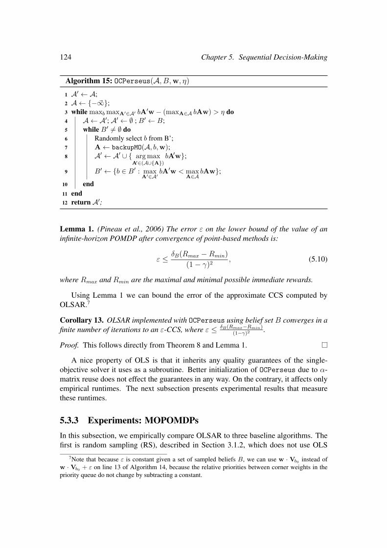
124 Chapter 5. Sequential Decision-Making
Algorithm 15: OCPerseus(A, B,w, η)
Input: A POMDP1 A′ ← A;2 A ← − ~∞;3 while maxb maxA′∈A′ bA
′w − (maxA∈A bAw) > η do4 A ← A′; A′ ← ∅ ; B′ ← B;5 while B′ 6= ∅ do6 Randomly select b from B’;7 A← backupMO(A, b,w);8 A′ ← A′ ∪ arg max
A′∈(A∪A)bA′w;
9 B′ ← b ∈ B′ : maxA′∈A′
bA′w < maxA∈A
bAw;
10 end11 end12 return A′;
Lemma 1. (Pineau et al., 2006) The error ε on the lower bound of the value of aninfinite-horizon POMDP after convergence of point-based methods is:
ε ≤ δB(Rmax −Rmin)
(1− γ)2, (5.10)
where Rmax and Rmin are the maximal and minimal possible immediate rewards.
Using Lemma 1 we can bound the error of the approximate CCS computed byOLSAR.7
Corollary 13. OLSAR implemented with OCPerseus using belief set B converges in afinite number of iterations to an ε-CCS, where ε ≤ δB(Rmax−Rmin)
(1−γ)2.
Proof. This follows directly from Theorem 8 and Lemma 1.
A nice property of OLS is that it inherits any quality guarantees of the single-objective solver it uses as a subroutine. Better initialization of OCPerseus due to α-matrix reuse does not effect the guarantees in any way. On the contrary, it affects onlyempirical runtimes. The next subsection presents experimental results that measurethese runtimes.
5.3.3 Experiments: MOPOMDPsIn this subsection, we empirically compare OLSAR to three baseline algorithms. Thefirst is random sampling (RS), described in Section 3.1.2, which does not use OLS
7Note that because ε is constant given a set of sampled beliefs B, we can use w · Vb0 instead ofw · Vb0 + ε on line 13 of Algorithm 14, because the relative priorities between corner weights in thepriority queue do not change by subtracting a constant.

5.3. OLS with Alpha Reuse for MOPOMDPs 125
1e-041e-021e+00
500 1000 1500 2000runtime (ms)
ε
1e-04
1e-01
1e+02
500 1000 1500 2000 2500runtime (ms)
ε
RS
RAR
OLS+
OLSAR
Figure 5.3: The error with respect to a reference set as a function of the runtime for(left) Tiger 2 and (right) Tiger3. The shaded regions represent standard error. Note thelog scale in the y-axis. In order to avoid clutter in the plot (due to the log-scale) weonly show the standard error above the lines.
or α-matrix reuse. The second is random sampling with alpha reuse (RAR), whichdoes not use OLS. The third is OLS+OCPerseus, which does not use α-matrix reuse.We do not present results for the augmented-state method of (White and Kim, 1980),as this it proved to be prohibitively computationally expensive for even the smallestproblems. We tested the algorithms on three MOPOMDPs based on the Tiger (Cassan-dra et al., 1994) and Maze20 (Hauskrecht, 2000) benchmark POMDPs. Because weuse infinite-horizon MOPOMDPs – which are undecidable – we cannot obtain the trueCCS. Therefore, we compare our algorithms’ solutions to reference sets obtained byrunning OLSAR with many more sampled belief points and η set 10 times smaller.
Multi-Objective Tiger
In the Tiger problem (Cassandra et al., 1994), an agent faces two doors: behind oneis a tiger and behind the other is treasure. The agent can listen or open one of thedoors. When it listens, it hears the tiger behind one of the doors. This observationis accurate with probability 0.85. Finding the treasure, finding the tiger, and listeningyield rewards of 10, 100, and -1, respectively. We use a discount factor of γ = 0.9.
While the single-objective Tiger problem assumes all three rewards are on the samescale, it is actually difficult in practice to quantify the trade-offs between, e.g., riskingan encounter with the tiger and acquiring treasure. In two-objective MO-Tiger (Tiger2),we assume that the treasure and the cost of listening are on the same scale but treatavoiding the tiger as a separate objective. In three-objective MO-Tiger (Tiger3), wetreat all three forms of reward as separate objectives.
We conducted 25 runs of each method on both Tiger2 and Tiger3. We ran allalgorithms with 100 belief points generated by random exploration, η = 1 × 10⁶, andb0 set to a uniform distribution. The reference set was obtained using 250 belief points.

126 Chapter 5. Sequential Decision-Making
On Tiger2 (Figure 5.3 (left)), OLS+OCPerseus converges in 0.87s on average, witha maximal error in scalarized value across the weight simplex w.r.t. the reference setof 5 × 10⁻⁶. OLSAR converges significantly faster (t-test: p < 0.01), in on average0.53s, with similar error 4×10⁻⁶ (this difference in error is not significant). RAR doesnot converge as it just keeps sampling new weights. However, we can measure errorw.r.t. the reference set. After 2s (about four times what OLSAR needs to converge),RAR has an error with respect to the reference set of 4.5× 10⁻³ (a factor of 103 higherthan OLSAR after convergence). RS is even worse and does not come further than a0.78 error after 2s. OLS+OCPerseus and OLSAR perform similarly in the first half:they use about the same time on the first four iterations (0.35s). However, OLSAR issignificantly faster for the second half. Thus, on Tiger2, OLS-based methods are sig-nificantly better than random sampling and α-reuse significantly speeds the discoveryof good value vectors.
The results for the Tiger3 problem are in Figure 5.3 (right). RS and RAR bothperform poorly, with RAR better by a factor of two. OLS+Perseus is faster than RARbut OLSAR is the fastest and converges in about 2s. OLS+OCPerseus eventually con-verges to the same error but takes 10 times longer. As before, OLS-based methods out-perform random sampling. Furthermore, for this 3-objective problem, α-reuse speedsconvergence of OLSAR by an order of magnitude.
We also compared three variations of OLSAR: using all previously found α-matrices,only reusing those found for the policy of the closest previous weight, and usingthose α-matrices for policies whose multi-objective values make up the current cornerweight. However, no significant differences where found between their convergencetimes or final error, neither in the 2- nor in the 3-objective Tiger problem.
Multi-Objective Maze20
In Maze20 (Hauskrecht, 2000), a robot must navigate through a 20-state maze. Ithas four actions to move in the cardinal directions, plus two sensing actions to per-ceive walls in the north-south or east-west directions. Transitions and observations arestochastic. In the single-objective problem, the agent gets reward of 2 for sensing, 4 formoving while avoiding the wall, and 150 for reaching the goal. In multi-objective Maze20 (MO-Maze20), the reward for reaching the goal is treated as a separate objective,yielding a two-objective problem.
To test performance of OLSAR on MO-Maze20, we first created a reference set byletting OLSAR converge using 1500 sampled beliefs. This took 11 hours. Then weran OLSAR, OLS+OCPerseus, RAR, and RS with 1000 sampled beliefs. Due to thecomputational expense, we conducted only three runs per method. Figure 5.4 showsthe results. OLSAR converges after (on average) 291 minutes (4.90hrs) at an errorof 0.09, less than 0.5% w.r.t. the reference set. We let OLS+OCPerseus run for 11hours but it did not converge in that time. OLS+OCPerseus, RS, and RAR have similarperformance after around 300 minutes. However, until then, OLS+OCPerseus doesbetter (and unlike RS and RAR, OLS+OCPerseus is guaranteed to converge). OLSAR

5.4. Conclusion 127
0.1
1.0
10.0
100 200 300 400runtime (min)
ε
RS
RAR
OLS+
OLSAR
Figure 5.4: The error with respect to a reference set as a function of the runtime forMO-Maze20. The shaded regions represent standard error. Note the log scale in they-axis. In order to avoid clutter in the plot (due to the log-scale) we only show thestandard error above the lines.
converges at significantly less error than what the other methods have attained after400 minutes. We therefore conclude that OLSAR reduces error more quickly than theother algorithms and converges faster than OLS+OCPerseus.
5.4 Conclusion
In this chapter we have proposed novel methods for multi-objective sequential decisionproblems, i.e., MOMDPs and MOPOMDPs, using the OLS framework of Chapter 3.First, we tackled a large MOMDP called the maintenance planning problem (MPP)using OLS-based methods. Second, we proposed a new method for infinite-horizonMOPOMDPs, that — as far as we are aware — is the first method to reasonably scale.
For the MPP, we have shown that it is possible to create multi-objective methodson the basis of OLS and state-of-the single-objective subroutines that are tailored forthe MPP. We have shown that it is easy to replace these subroutines if the state-of-the-art for a given problem improves. We compared exact CCS planning methods, i.e.,OLS+SPUDD and OLS+CoRe, to an approximate planning method, i.e., OLS+UCT∗.We showed that while the approximate subroutine does not provide bounds on thequality of approximation, OLS+UCT∗ can quickly produce approximate CCSs withlow error, ε, in practice. We therefore conclude that the OLS framework offers a flex-ible framework that is easy to use for large problems, especially when solvers for thescalarized, i.e., single-objective, versions of these problems already exist.
For MOPOMDPs, we proposed, analyzed, and tested OLSAR, a novel algorithmfor MOPOMDPs that intelligently selects a sequence of scalarized POMDPs, by build-ing on the OLS framework. OLSAR uses OCPerseus, a scalarized MOPOMDP solverthat returns the multi-objective value of the policies it finds, as well as the α-matrices

128 Chapter 5. Sequential Decision-Making
that describe them. A key insight underlying OLSAR is that these α-matrices canbe reused in subsequent calls to OCPerseus, greatly reducing runtimes in practice.Furthermore, because OCPerseus returns ε-optimal policies, OLSAR is guaranteed toreturn an ε-CCS. Our experiments show that OLSAR greatly outperforms alternativesthat do not use OLS and/or α-matrix reuse. We therefore conclude that OLS and reuseare key to keeping MOPOMDPs tractable.

Chapter 6Conclusion
In this dissertation, we aimed to answer the following question: “Can we create fastmulti-objective planning algorithms for cooperative decision problems that are: eithersingle- or multi-agent, single-shot or sequential, and fully or partially observable?”To answer this question affirmatively, we have discussed several models and proposedalgorithms for multi-objective decision-theoretic planning. In this final chapter, we firstreiterate our contributions and discuss their implications for the field of multi-objectivedecision theory in Section 6.1. In Section 6.2, we critically review our own work andoutline several possibilities for future research.
6.1 Contributions
In this section we summarize our contributions. Our contributions are two-fold; wehave made contributions that apply to cooperative multi-objective decision problemsin general, and we have made problem-specific contributions. We start with the bigpicture, and then go into the problem-specific contributions. For our contributions, webriefly discuss what we think the implications are for future research in this researchdirection.
6.1.1 The big picture
The research we presented in this dissertation is motivated by the need for solvingdecision-problems with multiple objectives; not only are there many real-world prob-lems that have multiple objectives, but we have also argued that these often cannot besolved with existing single-objective techniques, because it is often impossible to apriori scalarize, i.e., convert multi-objective problems to single-objective ones.
In order to make explicit under what circumstances special methods are needed tosolve multi-objective problems, we identified three scenarios in which it is impossible,infeasible, or undesirable to scalarize a priori in Chapter 1. As well as providing mo-
129

130 Chapter 6. Conclusion
tivation for the need for multi-objective methods, these scenarios also represent threemain ways these methods are applied in practice.
We proposed a taxonomy that classifies multi-objective methods according to theapplicable scenario, the scalarization function (which projects multi-objective valuesto scalar ones), and the type of policies that are allowed in Chapter 2. We showed howthese three aspects together determine the nature of an optimal solution, which can bea single policy, or a coverage set containing multiple policies. We limited our scope toproblems for which multiple policies are required.
Our taxonomy is based on a utility-based approach, which sees the scalarizationfunction as part of the utility, and thus part of the problem definition. This contrastswith the so-called axiomatic approach, which usually assumes the Pareto front is theappropriate solution. We showed that the utility-based approach can be used to jus-tify the choice for a solution set. Based on the utility-based approach we argued fora particular solution set: the convex coverage set (CCS), which applies to two impor-tant parts of the taxonomy. The first is the case in which the scalarization function islinear, i.e., the inner product of a vector of positive weights, w, and the vector-valuedvalue of a policy in a multi-objective decision problem, and the second is when thescalarization function is monotonically increasing in all objectives and stochastic poli-cies are allowed. The CCS is the central solution concept of this dissertation, andwe propose several novel planning algorithms for determining the CCS in a variety ofmulti-objective cooperative planning problems.
In Chapter 3, we discussed the two main approaches to create new CCS algorithmsbuilding from an existing single-objective planning algorithm. The first approach, thatis often taken in the literature, we refer to as the inner loop approach. In this ap-proach, the maximizations and summations — that are necessary to compute the opti-mal policy and policy value of a single-objective decision problem — inside the innermost loops of the single-objective algorithms are replaced with appropriate pruningoperators and cross-sums between sets of value vectors. Inner loop algorithms are asproblem-specific as the single-objective algorithms on which they are based. The sec-ond approach is the outer loop approach, in which a series of scalarized problems aresolved using the single-objective method as a subroutine in order to incrementally buildup the CCS for a multi-objective problem. Because these single-objective subroutinescan be left unchanged, outer loop methods are generic frameworks: they can apply toany (scalarizable) multi-objective decision problem. Important disadvantages of exist-ing outer loop methods however, include that they often do not converge to the exactCCS, except for in the limit, and that there are no quality bounds for the intermediateapproximate CCSs. Therefore, we propose a new outer loop method: the optimisticlinear support (OLS) framework.
The OLS framework takes inspiration from the POMDP literature (and specificallyCheng’s linear support algorithm (Cheng, 1988)), to exploit the piecewise linearityand convexity of the scalarized value function (under linear scalarization) in multi-objective decision problems. OLS is an outer loop approach, and thus solves a seriesof scalarized problems, for different (linear) scalarization weights w. At each itera-

6.1. Contributions 131
tion, OLS identifies the single weight vector w that can lead to the maximal possibleimprovement on a partial CCS it has already identified, and calls a single-objectivesubroutine to solve a scalarized instance of the problem for w. By doing so, OLSis guaranteed to terminate in a finite number of iterations. Furthermore, when thesingle-objective subroutine is exact, i.e., guaranteed to find the optimal policy for thescalarized instance of the problem, OLS is guaranteed to return the exact CCS. Beforetermination, OLS can bound the quality loss if the partial CCS it has identified so farwould be used to approximate the exact CCS, in terms of lost scalarized value. In otherwords, it is an anytime algorithm, for which each intermediate CCS is an ε-CCS. Wehave shown empirically (for MO-CoGs in Chapter 4) that it is often possible to producean ε-CCS in a fraction of the time it takes to produce an exact CCS, even for small ε.
When exact single-objective subroutines are not available, OLS can also functionin combination with approximate single-objective subroutines. When such an approx-imate subroutine produces a bounded approximation with at most ε error, OLS is guar-anteed to produce an ε-CCS upon termination. We have provided practical examplesof this in the context of MO-CoGs (Chapter 4) and MOPOMDPs (Chapter 5).
Often, OLS can be further improved by reusing the policies, value functions, orother artifacts produced by the single-objective subroutines during earlier iterationsof OLS to hot-start the single-objective subroutines in later iterations. The preciseinformation that can be reused depends on the problem. We have shown the reuse ofa representation of the value function in the form of α-matrices in MOPOMDPs to beparticularly effective in Chapter 5.
When we compare inner loop algorithms and OLS-based algorithms that use thesame single-objective methods as a basis/subroutine, we observe that inner loop algo-rithms typically scale better in the number of objective of a multi-objective decisionproblem, and OLS-based algorithms scale better in the size of the scalarized problems(such as the number of agents in a (MO-)CoG). We therefore conclude that inner loopand outer loop methods are complementary in this respect. However, the inner loopmethods are typically not anytime, and need to run until completion before producinga result. Additionally, contrary to inner loop methods, OLS imposes very little addi-tional memory demands in addition to the memory demands of the single-objectivesubroutines it employs. This can be a deciding factor when memory is limited, as wehave shown in the context of MO-CoGs in Chapter 4. Furthermore, while it is rela-tively easy to replace a subroutine in OLS (as we show for example in Chapter 5 in thecontext of large MOMDPs), it is typically far from trivial to create a new inner loopmethod based on a different single-objective algorithm.
We conclude that OLS is a framework that can be applied in the context of differ-ent multi-objective decision problems (with relatively little effort if a single-objectivesubroutine is available), is faster than corresponding inner loop methods for small andmedium objectives, and typically uses less memory than inner loop methods.
We believe that the advantages of OLS can be exploited in many future CCS plan-ning methods. Especially when real-world problems require the usage of problem-specific solution methods, we argue that OLS provides a fast and relatively low-effort

132 Chapter 6. Conclusion
option for creating a multi-objective solution method.
6.1.2 Problem-specific contributions
In this dissertation, we have made contributions to three classes of decision problems:multi-objective coordination graphs (MO-CoGs), multi-objective Markov decision pro-cesses (MOMDPs) and multi-objective partially observable Markov decision processes(MOPOMDPs).
Multi-objective coordination graphs
For MO-CoGs, we have proposed five novel algorithms: convex multi-objective vari-able elimination (CMOVE), convex AND/OR tree search (CTS), variable eliminationlinear support (VELS), AND/OR tree search linear support (TSLS) and variational op-timistic linear support (VOLS). The first two are inner loop methods, while the lastthree are outer loop methods that build on optimistic linear support (OLS).
We noted that it is possible to take the inner loop approach when building uponsingle-objective methods whose core operations consist of maximizations and summa-tions, such as variable elimination and AND/OR tree search. However, when the coreoperations are different, such as for variational methods — in which reparameteriza-tions and restructuring of the set of local payoff functions form the core operations —it is not clear how to take an inner loop approach. It is always possible to take an outerloop approach for MO-CoGs, as it can use a complete and unchanged single-objectivesolver as a subroutine, and evaluate the multi-objective value of joint actions that areproduced by this subroutine. An example of this is our VOLS algorithm, which buildson OLS and employs variational methods as subroutines. Because OLS inherits bothquality and memory guarantees from the single-objective subroutines it employs, OLSopens up the way to creating multi-objective methods with favorable quality and mem-ory properties from single-objective methods to which an inner loop approach doesnot apply. We consider this an important advantage in the context of MO-CoGs as itsscalarized version, i.e., the single-objective CoG1, is a large and active field of researchthat has produced many such methods. Furthermore, because it takes relatively littleeffort to plug in a new subroutine into OLS, it offers an attractive framework to createstate-of-the-art multi-objective methods.
We compared the inner loop methods we propose to their corresponding OLS-based methods. Specifically, we compared CMOVE to VELS and CTS to TSLS. Weshowed both theoretically and empirically that OLS-based methods scale better in thenumber of agents in terms of runtime, while inner loop methods scale better in thenumber of objectives. We showed — both theoretically and empirically — that OLS-based methods perform better overall in terms of memory requirements than inner loopmethods.
1Or equivalents of the CoG, such as finding the MAP in probabilistic graphical models (Pearl, 1988).

6.1. Contributions 133
We have shown that OLS-based algorithms are anytime, and that any intermediatesolution set during the execution of an OLS-based algorithm is an ε-CCS, as long asthe quality bounds of the single-objective method are known. We have used this resultto show empirically, e.g., using VELS, that we can produce ε-CCSs in a fraction ofthe runtime that is required to produce an exact CCS. Furthermore, when the single-objective subroutine, such as the variational subroutine in VOLS, is not exact, butdoes produce an ε-approximate solution, that OLS inherits this quality guarantee andcan produce an ε-CCS. This is a major advantage, as (MO-)CoGs are NP-hard, andtherefore most state-of-the-art solvers are approximate.
We have shown with VOLS, that it is possible to reuse parts of the solutions/artifactsproduced by single-objective variational subroutines in earlier iterations of OLS, in or-der to hot-start the variational subroutine in later iterations. Specifically, VOLS reusesthe restructured and reparameterized set of local payoff functions that variational meth-ods produce. We have shown empirically that this can lead to better runtime and/orquality results.
When we compare our outer and inner loop methods in terms of runtime, mem-ory usage, and quality guarantees, we note that exact methods (CMOVE, CTS, VELSand TSLS) have runtimes that depend exponentially on the induced width. Of theseexact methods, VELS is typically fastest and when the number of objectives is low ormedium, and TSLS is most memory-efficient. For higher number of objectives, innerloop methods are typically faster than outer loop methods; CMOVE scales better thanVELS in the number of objectives, but has poor memory guarantees; CTS has bettermemory usage than CMOVE but is slower. OLS-based outer loop methods are alwaysmore memory-efficient than their inner loop counterparts. Compared to exact methods,VOLS scales much better in the number of agents, i.e., the runtime does not increaseexponentially with the number of agents. However, VOLS only produces an ε-CCS.
Summarizing, we have proposed an analyzed five novel algorithms for MO-CoGsthat compute a (approximate) CCS. Our methods offer different trade-offs betweenruntime, memory usage, and quality guarantees.
Multi-objective MDPs
For MOMDPs, we have demonstrated the efficacy of OLS when the MOMDP is verylarge. In order to illustrate this we have made use of the maintenance planning problem(MPP) (Scharpff et al., 2013; Roijers et al., 2014a; Scharpff et al., 2015, 2016). TheMPP is notoriously hard due to its large state and action space. Therefore, the exist-ing methods for the single-objective version of the MPP exploit the specific problemstructure of the MPP; the SPUDD and UCT∗ algorithms employ a problem-specific en-coding (Scharpff et al., 2013) while the CoRe algorithm (Scharpff et al., 2016) — thatwas proposed only recently — exploits the transition independence between featuresof the state-space.
We have shown that it possible to create planning methods that compute the CCSfor problems like the MPP by using state-of-the-art, possibly problem-specific, single-

134 Chapter 6. Conclusion
objective solvers as subroutines inside OLS. Because it is relatively easy to exchangesubroutines (but not to create inner loop methods from new single-objective methods),we conclude that especially for problems that require a problem-specific approach,OLS is key to the creation of effective multi-objective planning methods.
Multi-objective POMDPs
In this dissertation, we proposed, analyzed, and tested optimistic linear support withalpha reuse (OLSAR). Because OLSAR uses the OLS framework, it intelligently se-lects a sequence of scalarized POMDPs to solve in order to solve MOPOMDPs. Asfar was we are aware, this is the first MOPOMDP planning method that computes theCCS and reasonably scales in the number of states of the MOPOMDP.
We have shown how to represent the value function (in the belief b and the scalar-ization weight w) in terms of α-matrices. OLSAR uses this representation. The single-objective subroutine we propose for OLSAR is OLS-compliant Perseus (OCPerseus),a scalarized MOPOMDP solver that returns the multi-objective value of the policiesit finds, as well as the α-matrices that describe them. A key insight underlying OL-SAR is that the α-matrices produced by OCPerseus can be reused in subsequent callsto OCPerseus. This α-reuse greatly reduces runtimes in practice. Furthermore, sinceOCPerseus returns ε-optimal policies, OLSAR is guaranteed in turn to return an ε-CCS. Our experimental results show that OLSAR greatly outperforms alternatives thatdo not use OLS and/or α-matrix reuse.
6.2 Discussion and Future Work
In this section, we critically review the work in this dissertation, and identify opportu-nities for future work.
6.2.1 On the sufficiency of the taxonomy
In Chapter 2, we introduced a taxonomy based on the utility-based approach. Weassumed the existence of a utility or scalarization function, f .
In this dissertation we have restricted f to monotonically increasing functions inall objectives. We argue that this is a minimal assumption because it simply statesthat increasing the value with respect to one objective without diminishing the others,cannot decrease the scalarized value. This — in our view — corresponds to what wemean by ‘objective’. However, it is possible to have a preference ordering over valuevectors, without there being an f that corresponds to it. When preference is based on alexicographical ordering, i.e., even an infinitesimal improvement in an objective with ahigher priority is better than a large improvement in an objective with a lower priority,and the rewards are vectors in <n, there is no f : <n → < that corresponds to this

6.2. Discussion and Future Work 135
(Sen, 1995). Therefore, lexicographical orderings falls outside of our mathematicalformalism.
We have used one special case of f , namely the linear (and monotonically increas-ing) scalarization function. However, there are more special cases of f correspondingto different preference orderings described in the literature. For example, when certain“fairness” constraints are imposed on f this leads to the Lorenz front (Perny et al.,2013), which is a subset of the Pareto front. We have not identified this, or other, ad-ditional constraints that can be imposed on f . However, it would be useful for futurework in multi-objective decision making to have an overview of such constraints, andespecially in what type of situations they occur.
6.2.2 Scalarized expectation of return versus expectation of scalar-ized return
In Section 1.1 in Definition 1, we defined the scalarized value of a policy, π, to bethe result of applying the scalarization function f to the multi-objective value Vπ,i.e., V π
w(s) = f(Vπ(s),w). Since Vπ(s) is typically itself an expectation, this meansthat the scalarization function is applied after the expectation is computed, e.g., forMOMDPs (Definition 33):
V πw(s) = f(Vπ(s),w) = f(E[
∞∑k=0
γkrk | π, s0 = s],w).
This formulation, which we refer to as the scalarization of the expected return (SER)is standard in the literature. However, it is not the only conceivable option. It is alsopossible to define V π
w(s) as the expectation of the scalarized return (ESR), e.g., forMOMDPs:
V πw(s) = E[f(
∞∑k=0
γkrk,w) | π, s0 = s]
Which definition is used can critically affect which policies are preferred. Forexample, consider the following 2-objective infinite-horizon MOMDP, illustrated inFigure 6.1. There are four states (A, B, C, and D). The agent starts in state A and hastwo possible actions: a1 transits to state B or C, each with probability of 0.5, and a2
transits to state D with probability 1. Both actions lead to a (0, 0) reward. In states B,C and D there is only one action, which leads to a deterministic reward of (3, 0) for B,(0, 3) for C, and (1, 1) for D.
The scalarization function just multiplies the two objectives together if the value inboth objectives is greater than 0, and is 0 otherwise. Thus for this MOMDP with onlypositive rewards, the scalarized value under SER is,
V πw(s) = V π
1 (s)V π2 (s),
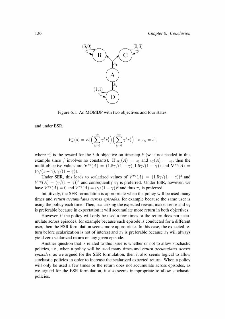
136 Chapter 6. Conclusion
A
B C
D
(0,3)(3,0)
(1,1)
a
a
1
2
Figure 6.1: An MOMDP with two objectives and four states.
and under ESR,
V πw(s) = E[
( ∞∑k=0
γkr1k
)( ∞∑k=0
γkr2k
)| π, s0 = s],
where rik is the reward for the i-th objective on timestep k (w is not needed in thisexample since f involves no constants). If π1(A) = a1 and π2(A) = a2, then themulti-objective values are Vπ1(A) = (1.5γ/(1 − γ), 1.5γ/(1 − γ)) and Vπ2(A) =(γ/(1− γ), γ/(1− γ)).
Under SER, this leads to scalarized values of V π1(A) = (1.5γ/(1 − γ))2 andV π2(A) = (γ/(1 − γ))2 and consequently π1 is preferred. Under ESR, however, wehave V π1(A) = 0 and V π2(A) = (γ/(1− γ))2 and thus π2 is preferred.
Intuitively, the SER formulation is appropriate when the policy will be used manytimes and return accumulates across episodes, for example because the same user isusing the policy each time. Then, scalarizing the expected reward makes sense and π1
is preferable because in expectation it will accumulate more return in both objectives.However, if the policy will only be used a few times or the return does not accu-
mulate across episodes, for example because each episode is conducted for a differentuser, then the ESR formulation seems more appropriate. In this case, the expected re-turn before scalarization is not of interest and π2 is preferable because π1 will alwaysyield zero scalarized return on any given episode.
Another question that is related to this issue is whether or not to allow stochasticpolicies, i.e., when a policy will be used many times and return accumulates acrossepisodes, as we argued for the SER formulation, then it also seems logical to allowstochastic policies in order to increase the scalarized expected return. When a policywill only be used a few times or the return does not accumulate across episodes, aswe argued for the ESR formulation, it also seems inappropriate to allow stochasticpolicies.

6.2. Discussion and Future Work 137
To our knowledge, there is no literature on multi-objective decision-theoretic plan-ning and learning that employs the ESR formulation, even though there are many real-world scenarios in which it seems more appropriate. For example, in the medicalapplication of Lizotte et al. (2010), each patient gets only one episode to treat his orher illness, and needs to balance the effectiveness of the treatment against the severityof the side-effects. Therefore, the patient clearly interested in maximizing ESR, notSER. Thus, we believe that developing methods for the ESR formulation is a criticaldirection for future research in multi-objective decision making.
6.2.3 Other decision problemsFor the MO-CoG, MOMDP and MOPOMDP models we propose new algorithms.However, there are more possible collaborative MODPs, that extend SODPs from Fig-ure 2.2 that have been studied in the literature. We briefly discuss those models here,and how they are related to the previously discussed MODPs.
Firstly, collaborative Bayesian games (CBGs) (Oliehoek et al., 2012) are single-shot, multi-agent models like CoGs. Unlike CoGs however, each agent receives aprivate observation, called a type θ, before it needs to act. The distributions over typesfor each agent are common knowledge. Deterministic policies in a CBG specify foran action for each agent for every type of that agent. CBGs can be flattened to a largeCoG by for enumerating the possible mappings from types to actions for each agent andseeing these mappings as that agent’s local action space,Ai. This same reduction couldbe made for a multi-objective version of a CBG to a MO-CoG. CBGs are often used asa subproblem in the sequential version of the problem, the Dec-POMDP (MacDermedand Isbell, 2013).
The class of multi-agent, sequential, and partially observable collaborative mod-els is called the multi-agent Markov decision process (MMDP) model in the single-objective-setting. Similar to flattening a CoG into a BP, by treating the team of agentsas one central agent with a very large action space, an MMDP can be flattened to a verylarge MDP, as we have mentioned in Section 5.2 for the maintenance planning prob-lem. However, the joint state and action spaces of an MMDP are exponentially sizedin the number of agents, so solving an MMDP in such a centralized manner, is typi-cally infeasible. Therefore, MMDPs can — in general — only be exactly solved forsmall numbers of agents (e.g., Scharpff et al. (2015)). For larger MMDPs, approximatemethods are required. These approximate methods — an overview of which is givenby Spaan et al. (2011) — either rely on an artificial factorization of the value func-tion (Guestrin et al., 2002), or decentralization, which leads to a partially observableproblem setting. At present, decentralized approximation methods typically do notprovide bounds with respect to the approximation quality due to decentralization. Itmay be an interesting research possibility to try and construct methods that do providesuch bounds. Once such methods are invented, their quality bounds will immediatelytransfer to the multi-objective setting, when they are used as a subroutine inside OLS.
The class of multi-agent, sequential, and partially observable collaborative mod-

138 Chapter 6. Conclusion
els is known as the decentralized partially observable Markov decision process (Dec-POMDP) (Bernstein et al., 2002; Oliehoek, 2010) model in the single-objective setting.Recently, major strides in solving Dec-POMDPs have been made. In particular, it hasbeen shown that there is a reduction from Dec-POMDP to a special type of centralizedPOMDP called a non-observable Markov decision process (NOMDP) (MacDermedand Isbell, 2013; Nayyar et al., 2013; Dibangoye et al., 2013; Oliehoek and Amato,2014). This allows POMDP solution methods to be employed in the context of Dec-POMDPs. For multi-objective Dec-POMDPs (MO-Dec-POMDPs), the reduction toNOMDPs is potentially very useful as well. Specifically, an equivalent reduction froman MO-Dec-POMDP to a multi-objective NOMDP (MONOMDP) could be made, forwhich the OLSAR algorithm that we propose for MOPOMDPs in Section 5.3 wouldapply.
6.2.4 Other aspects of decision problemsAside from the aspects that are discussed in Section 1.3, there are several other orthog-onal aspects that are studied in the literature, such as continuous time (Van Hasselt,2012; de Sousa Messias, 2014) and non-Markovian states (Das et al., 1999). Theseaspects are in principle compatible with our approach. Models in which there aremultiple self-interested or even adversarial agents (Brown et al., 2012; Wiggers et al.,2015) however, are not compatible with our approach, as Assumption 1 — on whichour methods rely — does not hold in these settings. It would be interesting to investi-gate whether an outer loop approach may still be interesting in self-interested settingsby analyzing the properties of the scalarized value function of these problems.
6.2.5 Reuse in OLS and scalability in the number of objectivesAs we have mentioned several times in this dissertation, OLS works well when thenumber of objectives is low. OLS scales poorly in the number of objectives becausethe number of calls to the single objective solver depends on the number of cornerweights, which is exponential in the number of objectives (Theorem 5).
As we have seen in Section 5.3, when we employ reuse (Section 3.6), the effort forcorner weights for which no new value is found can be drastically reduced in practiceby hot-starting the single-objective subroutine. For MOPOMDPs this is even vital tokeep the planning problem tractable.
In this dissertation, we have not yet made a theoretical analysis of the effect ofreuse and its effect on the scalability in the number of objectives. Intuitively, when thesingle-objective method terminates immediately after a hot-start when no new valuevector can be identified this reduces the runtime to the runtime of the single-objectivesolver times the number of solutions in the final CCS. In practice however, the single-objective solver will need some time to determine whether improvements can be found.Furthermore, as we have seen in VOLS in Section 4.4.6, reuse is not always guaranteedto improve the runtime for every run of the single-objective solver.

6.2. Discussion and Future Work 139
In future work, we aim to provide an analysis of the effect of reuse upon runtime— and specifically on the scalability in the number of objectives — in different OLS-based methods when it can be proven that: the single-objective solver used terminatesin one iteration (as in OLSAR) or when an extra check to confirm the optimality ofa partial CCS for a new w can be introduced, and that reuse can only improve theruntime of the single-objective solver.
6.2.6 Decision makers in the loopIn this dissertation we have assumed that we know the constraints on the scalarizationfunction, f , produce a coverage set by running a planning algorithm, and only in aseparate selection phase present that coverage set to the decision maker. There arehowever two issues with this workflow: first, the coverage set might be too large for adecision maker to analyze, and second, we might be doing a lot of unnecessary workbecause the constraints on f are too loose.
An interesting way to mitigate both issues is to involve the decision maker whileplanning, i.e., when we produce intermediate results during the planning phase, wemight elicit more preference information from the decision maker by asking questionsabout these intermediate results (Benabbou and Perny, 2015). We believe that thisparticularly compatible with OLS, as decision makers can be presented with values ofcomplete policies from the partial CCS, S, between iterations of OLS. The answersthat the user provides can be used by OLS to quickly reduce the interesting region ofthe weight space, leading to large speed ups.


Bibliography
Altman, E. (2002). Applications of markov decision processes in communication net-works. In Handbook of Markov decision processes, pages 489–536. Springer.
Arnborg, S. (1985). Efficient algorithms for combinatorial problems on graphs withbounded decomposability — a survey. BIT Numerical Mathematics, 25(1):1–23.
Astrom, K. J. (1965). Optimal control of Markov processes with incomplete stateinformation. Journal of Mathematical Analysis and Applications, 10(1):174–205.
Auer, P. and Ortner, R. (2010). UCB revisited: Improved regret bounds for the stochas-tic multi-armed bandit problem. Periodica Mathematica Hungarica, 61(1-2):55–65.
Avis, D. and Devroye, L. (2000). Estimating the number of vertices of a polyhedron.Information processing letters, 73(3):137–143.
Barrett, L. and Narayanan, S. (2008). Learning all optimal policies with multiplecriteria. In ICML 2008: Proceedings of The Twenty-fifth International Conferenceon Machine Learning, pages 41–47.
Bayardo, R. J. J. and Miranker, D. P. On the space-time trade-off in solving constraintsatisfaction problems. In IJCAI 1995: Proceedings of the Fourteenth InternationalJoint Conference on Artificial Intelligence, pages 558–562.
Becker, R., Zilberstein, S., Lesser, V., and Goldman, C. (2003). Transition-IndependentDecentralized Markov Decision Processes. In AAMAS 2003: Proceedings of the Sec-ond International Joint Conference on Autonomous Agents and Multiagent Systems,pages 41–48.
Bellman, R. (1957a). Dynamic Programming. Princeton University Press, Princeton,New Jersey, USA.
Bellman, R. E. (1957b). A Markovian decision process. Journal of Mathematics andMechanics, 6:679–684.
141

142 BIBLIOGRAPHY
Benabbou, N. and Perny, P. (2015). Incremental weight elicitation for multiobjectivestate space search. In AAAI 2015: Proceedings of the Twenty-Ninth AAAI Confer-ence on Artificial Intelligence, pages 1093–1099.
Bergemann, D. and Valimaki, J. (2006). Efficient dynamic auctions. Cowles Founda-tion Discussion Paper.
Bernstein, D. S., Givan, R., Immerman, N., and Zilberstein, S. (2002). The complexityof decentralized control of Markov decision processes. Mathematics of operationsresearch, 27(4):819–840.
Bertsimas, D. and Tsitsiklis, J. (1997). Introduction to Linear Optimization. AthenaScientific, Nashua (NH), USA.
Bishop, C. M. (2006). Pattern Recognition and Machine Learning. Springer, NewYork (NY), USA.
Boutilier, C. (1996). Planning, learning and coordination in multiagent decision pro-cesses. In TARK 1996: Proceedings of the 6th conference on Theoretical aspects ofrationality and knowledge, pages 195–210.
Boutilier, C., Dean, T., and Hanks, S. (1999). Decision-theoretic planning: Structuralassumptions and computational leverage. Journal of Artificial Intelligence Research,11:1–94.
Brown, M., An, B., Kiekintveld, C., Ordonez, F., and Tambe, M. (2012). Multi-objective optimization for security games. In AAMAS 2012: Proceedings of the 11thInternational Conference on Autonomous Agents and Multiagent Systems-Volume 2,pages 863–870.
Busoniu, L., Babuska, R., and De Schutter, B. (2008). A comprehensive survey ofmultiagent reinforcement learning. IEEE Transactions on Systems, Man, and Cy-bernetics, 38(2):156–172.
Cassandra, A., Littman, M., and Zhang, N. (1997). Incremental pruning: A simple,fast, exact method for partially observable Markov decision processes. In UAI 1997:Proceedings of the Thirteenth Conference on Uncertainty in Artificial Intelligence,pages 54–61.
Cassandra, A. R. (1998). Exact and approximate algorithms for partially observableMarkov decision processes. PhD thesis, Brown University.
Cassandra, A. R., Kaelbling, L. P., and Littman, M. L. (1994). Acting optimally inpartially observable stochastic domains. In AAAI 1994: Proceedings of the TwelfthNational Conference on Artificial Intelligence, pages 1023–1028.
BIBLIOGRAPHY 143
Cavallo, R. (2008). Efficiency and redistribution in dynamic mechanism design. InEC 2008: Proceedings of the 9th ACM conference on electronic commerce, pages220–229.
Cheng, H.-T. (1988). Algorithms for partially observable Markov decision processes.PhD thesis, University of British Columbia, Vancouver.
Clemen, R. T. (1997). Making Hard Decisions: An Introduction to Decision Analysis.South-Western College Pub, 2 edition.
Das, T. K., Gosavi, A., Mahadevan, S., and Marchalleck, N. (1999). Solving semi-Markov decision problems using average reward reinforcement learning. Manage-ment Science, 45(4):560–574.
de Sousa Messias, J. V. T. (2014). Decision-Making under Uncertainty for Real RobotTeams. PhD thesis, Instituto Superior Tecnico, Lisbon, Portugal.
Dechter, R. (1998). Bucket elimination: A unifying framework for probabilistic infer-ence. In Learning in graphical models, pages 75–104. Springer Netherlands.
Dechter, R. (2013). Reasoning with Probabilistic and Deterministic Graphical Mod-els: Exact Algorithms, volume 7 of Synthesis Lectures on Artificial Intelligence andMachine Learning. Morgan & Claypool Publishers.
Dechter, R. and Mateescu, R. (2007). AND/OR search spaces for graphical models.Artificial intelligence, 171(2):73–106.
Delle Fave, F., Stranders, R., Rogers, A., and Jennings, N. (2011). Bounded decen-tralised coordination over multiple objectives. In Proceedings of the Tenth Inter-national Joint Conference on Autonomous Agents and Multiagent Systems, pages371–378.
Dibangoye, J. S., Amato, C., Buffet, O., and Charpillet, F. (2013). Optimally solv-ing Dec-POMDPs as continuous-state MDPs. In IJCAI 2013: Proceedings of theTwenty-Second International Joint Conference on Artificial Intelligence.
Drugan, M. M. and Nowe, A. (2013). Designing multi-objective multi-armed banditsalgorithms: A study. In IJCNN 2013: Proceedings of the 2013 International JointConference on Neural Networks, pages 1–8.
Dubus, J., Gonzales, C., and Perny, P. (2009a). Choquet optimization using GAI net-works for multiagent/multicriteria decision-making. In ADT 2009: Proceedings ofthe First International Conference on Algorithmic Decision Theory, pages 377–389.
Dubus, J., Gonzales, C., and Perny, P. (2009b). Multiobjective optimization usingGAI models. In IJCAI 2009: Proceedings of the Twenty-third International JointConference on Artificial Intelligence, pages 1902–1907.

144 BIBLIOGRAPHY
Feng, Z. and Zilberstein, S. (2004). Region-based incremental pruning for POMDPs.In UAI 2004: Proceedings of the Twentieth Conference on Uncertainty in ArtificialIntelligence, pages 146–153.
Franklin, S. and Graesser, A. (1997). Is it an agent, or just a program?: A taxonomyfor autonomous agents. In Intelligent agents III agent theories, architectures, andlanguages, pages 21–35. Springer.
Furcy, D. and Koenig, S. (2005). Limited discrepancy beam search. In IJCAI 2005:Proceedings of the Nineteenth International Joint Conference on Artificial Intelli-gence, pages 125–131.
Gonzales, C. and Perny, P. (2004). GAI networks for utility elicitation. In AAAI:Proceedings of the Nineteenth National Conference on Artificial Intelligence, pages224–234.
Graham, R. L. (1972). An efficient algorithm for determining the convex hull of afinite planar set. Information processing letters, 1(4):132–133.
Guestrin, C., Koller, D., and Parr, R. (2002). Multiagent planning with factored MDPs.In NIPS 2002: Advances in Neural Information Processing Systems 15, pages 1523–1530.
Guizzo, E. (2011). How Google’s self-driving car works. IEEE Spectrum Online,October, 18.
Handa, H. (2009a). EDA-RL: Estimation of distribution algorithms for reinforcementlearning problems. In GECCO 2009: ACM/SIGEVO Genetic and EvolutionaryComputation Conference, pages 405–412.
Handa, H. (2009b). Solving multi-objective reinforcement learning problems by EDA-RL - acquisition of various strategies. In ISDA 2009: Proceedings of the NinthInternatonal Conference on Intelligent Sysems Design and Applications, pages 426–431.
Hauskrecht, M. (2000). Value-function approximations for partially observableMarkov decision processes. Journal of Artificial Intelligence Research, 13:33–94.
Henk, M., Richter-Gebert, J., and Ziegler, G. M. (1997). Basic properties of convexpolytopes. In Handbook of Discrete and Computational Geometry, Ch.13, pages243–270. CRC Press, Boca.
Hoey, J., St-Aubin, R., Hu, A., and Boutilier, C. (1999). SPUDD: Stochastic planningusing decision diagrams. In UAI 1999: Proceedings of the Fifteenth conference onUncertainty in artificial intelligence, pages 279–288.
BIBLIOGRAPHY 145
Howard, R. A. (1960). Dynamic programming and Markov decision processes. MITPress.
Ihler, A. T., Flerova, N., Dechter, R., and Otten, L. (2012). Join-graph based cost-shifting schemes. In UAI 2012: Proceedings of the Twenty-Eighth Annual Confer-ence on Uncertainty in Artificial Intelligence, pages 397–406.
Inja, M., Kooijman, C., de Waard, M., Roijers, D. M., and Whiteson, S. (2014). QueuedPareto local search for multi-objective optimization. In PPSN 2014: Proceedings ofthe Thirteenth International Conference on Parallel Problem Solving from Nature,pages 589–599.
Jarvis, R. A. (1973). On the identification of the convex hull of a finite set of points inthe plane. Information Processing Letters, 2(1):18–21.
Kaelbling, L., Littman, M., and Cassandra, A. (1998). Planning and acting in partiallyobservable stochastic domains. Artificial Intelligence, 101:99–134.
Kaibel, V. and Pfetsch, M. E. (2003). Some algorithmic problems in polytope theory.In Algebra, Geometry and Software Systems, pages 23–47. Springer.
Keller, T. and Eyerich, P. (2012). PROST: Probabilistic Planning Based on UCT. InICAPS 2012: Proceedings of the Twenty-Second International Conference on Auto-mated Planning and Scheduling, pages 119–127.
Keller, T. and Helmert, M. (2013). Trial-based heuristic tree search for finite horizonMDPs. In ICAPS 2013: Proceedings of the Twenty-Third International Conferenceon Automated Planning and Scheduling, pages 135–143.
Ketter, W., Peters, M., and Collins, J. (2013). Autonomous agents in future energymarkets: the 2012 power trading agent competition. In BNAIC 2013: Proceedingsof the 25th Benelux Conference on Artificial Intelligence, pages 328–329.
Kim, I. Y. and de Weck, O. L. (2005). Adaptive weighted-sum method for bi-objectiveoptimization: Pareto front generation. Structural and multidisciplinary optimization,29(2):149–158.
Kober, J. and Peters, J. (2012). Reinforcement learning in robotics: A survey. InWiering, M. A. and Van Otterlo, M., editors, Reinforcement Learning: State-of-the-Art, volume 12 of Adaptation, Learning, and Optimization, pages 579–610. SpringerBerlin/Heidelberg.
Kocsis, L. and Szepesvari, C. (2006). Bandit based Monte-Carlo planning. In MachineLearning: ECML 2006, pages 282–293.
Kok, J. and Vlassis, N. (2006). Collaborative multiagent reinforcement learning bypayoff propagation. Journal of Machine Learning Research, 7:1789–1828.

146 BIBLIOGRAPHY
Kok, J. R. and Vlassis, N. (2004). Sparse cooperative Q-learning. In ICML 2004:Proceedings of the twenty-first international conference on Machine learning, pages61–68.
Koller, D. and Friedman, N. (2009). Probabilistic Graphical Models: Principles andTechniques. MIT Press.
Kooijman, C., de Waard, M., Inja, M., Roijers, D. M., and Whiteson, S. (2015). Paretolocal policy search for MOMDP planning. In ESANN 2015: Special Session onEmerging Techniques and Applications in Multi-Objective Reinforcement Learningat the European Symposium on Artificial Neural Networks, Computational Intelli-gence and Machine Learning 2015, pages 53–58.
Kuleshov, V. and Precup, D. (2014). Algorithms for multi-armed bandit problems.arXiv preprint arXiv:1402.6028.
Kurniawati, H., Hsu, D., and Lee, W. (2008). SARSOP: Efficient point-based POMDPplanning by approximating optimally reachable belief spaces. In Robotics: Scienceand Systems.
Liu, Q. and Ihler, A. (2013). Variational algorithms for marginal MAP. Journal ofMachine Learning Research, 14:3165–3200.
Liu, Q. and Ihler, A. T. (2011). Bounding the partition function using Holder’s inequal-ity. In ICML 2011: Proceedings of the 28th International Conference on MachineLearning, pages 849–856.
Lizotte, D., Bowling, M., and Murphy, S. (2010). Efficient reinforcement learningwith multiple reward functions for randomized clinical trial analysis. In ICML 2010:Proceedings of the 27th International Conference on Machine Learning, pages 695–702.
MacDermed, L. C. and Isbell, C. (2013). Point based value iteration with optimal beliefcompression for Dec-POMDPs. In NIPS 2013: Advances in Neural InformationProcessing Systems 26, pages 100–108.
Madani, O., Hanks, S., and Condon, A. (2003). On the undecidability of probabilis-tic planning and related stochastic optimization problems. Artificial Intelligence,147(1):5–34.
Manne, A. S. (1960). Linear programming and sequential decisions. ManagementScience, 6(3):259–267.
Marinescu, R. (2008). AND/OR Search Strategies for Combinatorial Optimization inGraphical Models. PhD thesis, University of California, Irvine.

BIBLIOGRAPHY 147
Marinescu, R. (2009). Exploiting problem decomposition in multi-objective constraintoptimization. In CP 2009: Principles and Practice of Constraint Programming,pages 592–607.
Marinescu, R. (2011). Efficient approximation algorithms for multi-objective con-straint optimization. In ADT 2011: Proceedings of the Second International Con-ference on Algorithmic Decision Theory, pages 150–164.
Marinescu, R., Razak, A., and Wilson, N. (2012). Multi-objective influence diagrams.In UAI 2012: Proceedings of the Twenty-Eighth Conference on Uncertainty in Arti-ficial Intelligence, pages 574–583.
Mateescu, R. and Dechter, R. (2005). The relationship between AND/OR search andvariable elimination. In UAI 2005: Proceedings of the Twenty-First Conference onUncertainty in Artificial Intelligence, pages 380–387.
McMullen, P. (1970). The maximum numbers of faces of a convex polytope. Mathe-matika, 17(2):179–184.
Moffaert, K. V. and Nowe, A. (2014). Multi-objective reinforcement learning us-ing sets of Pareto dominating policies. Journal of Machine Learning Research,15:3483–3512.
Monahan, G. (1982). State of the art — a survey of partially observable Markov deci-sion processes: theory, models, and algorithms. Management Science, 28(1):1–16.
Monostori, L., Vancza, J., and Kumara, S. R. (2006). Agent-based systems for manu-facturing. CIRP Annals-Manufacturing Technology, 55(2):697–720.
Nair, R., Varakantham, P., Tambe, M., and Yokoo, M. (2005). Networked distributedPOMDPs: A synthesis of distributed constraint optimization and POMDPs. In AAAI2005: Proceedings of the Twentieth National Conference on Artificial Intelligence,pages 133–139.
Nayyar, A., Mahajan, A., and Teneketzis, D. (2013). Decentralized stochastic controlwith partial history sharing: A common information approach. IEEE Transactionson Automatic Control, 58:1644–1658.
Oliehoek, F. A. (2010). Value-based planning for teams of agents in stochastic partiallyobservable environments. PhD thesis, University of Amsterdam.
Oliehoek, F. A. and Amato, C. (2014). Dec-POMDPs as non-observable MDPs. IAStechnical report IAS-UVA-14-01, Amsterdam, The Netherlands.
Oliehoek, F. A., Spaan, M. T. J., and Witwicki, S. (2015). Factored upper bounds formultiagent planning problems under uncertainty with non-factored value functions.pages 1645–1651.

148 BIBLIOGRAPHY
Oliehoek, F. A., Whiteson, S., and Spaan, M. T. J. (2012). Exploiting structure in coop-erative Bayesian games. In UAI 2012: Proceedings of the Twenty-Eighth Conferenceon Uncertainty in Artificial Intelligence, pages 654–664.
Ong, S. C. W., Png, S. W., Hsu, D., and Lee, W. S. (2010). Planning under uncertaintyfor robotic tasks with mixed observability. The International Journal of RoboticsResearch, 29(8):1053–1068.
Pardoe, D. M. (2011). Adaptive trading agent strategies using market experience. PhDthesis, University of Texas at Austin.
Pearl, J. (1988). Probabilistic Reasoning In Intelligent Systems: Networks of PlausibleInference. Morgan Kaufmann.
Perny, P., Weng, P., Goldsmith, J., and Hanna, J. P. (2013). Approximation of Lorenz-optimal solutions in multiobjective Markov decision processes. In UAI 2013: Pro-ceedings of the Twenty-Ninth Conference on Uncertainty In Artificial Intelligence,pages 508–517.
Pineau, J., Gordon, G., and Thrun, S. (2006). Anytime point-based approximations forlarge POMDPs. Journal of Artificial Intelligence Research, 27:335–380.
Poupart, P., Kim, K., and Kim, D. (2011). Closing the gap: Improved bounds onoptimal POMDP solutions. In ICAPS 2011: Proceedings of the Twenty-First Inter-national Conference on Automated Planning and Scheduling, pages 194–201.
Puterman, M. L. (1994). Markov decision processes: discrete stochastic dynamic pro-gramming. John Wiley & Sons.
Roijers, D. M., Scharpff, J., Spaan, M. T., Oliehoek, F. A., de Weerdt, M., and White-son, S. (2014a). Bounded approximations for linear multi-objective planning underuncertainty. In ICAPS 2014: Proceedings of the Twenty-Fourth International Con-ference on Automated Planning and Scheduling, pages 262–270.
Roijers, D. M., Vamplew, P., Whiteson, S., and Dazeley, R. (2013a). A survey of multi-objective sequential decision-making. Journal of Artificial Intelligence Research,47:67–113.
Roijers, D. M., Whiteson, S., Ihler, A. T., and Oliehoek, F. A. (2015a). Variationalmulti-objective coordination. In MALIC 2015: NIPS Workshop on Learning, Infer-ence and Control of Multi-Agent Systems.
Roijers, D. M., Whiteson, S., and Oliehoek, F. (2013b). Computing convex coveragesets for multi-objective coordination graphs. In ADT 2013: Proceedings of the ThirdInternational Conference on Algorithmic Decision Theory, pages 309–323.
BIBLIOGRAPHY 149
Roijers, D. M., Whiteson, S., and Oliehoek, F. A. (2013c). Multi-objective variableelimination for collaborative graphical games. In AAMAS 2013: Proceedings ofthe Twelfth International Joint Conference on Autonomous Agents and MultiagentSystems, pages 1209–1210. Extended Abstract.
Roijers, D. M., Whiteson, S., and Oliehoek, F. A. (2014b). Linear support for multi-objective coordination graphs. In AAMAS 2014: Proceedings of the Thirteenth Inter-national Joint Conference on Autonomous Agents and Multi-Agent Systems, pages1297–1304.
Roijers, D. M., Whiteson, S., and Oliehoek, F. A. (2015b). Computing convex cov-erage sets for faster multi-objective coordination. Journal of Artificial IntelligenceResearch, 52:399–443.
Roijers, D. M., Whiteson, S., and Oliehoek, F. A. (2015c). Point-based planning formulti-objective POMDPs. In IJCAI 2015: Proceedings of the Twenty-Fourth Inter-national Joint Conference on Artificial Intelligence, pages 1666–1672.
Roijers, D. M., Whiteson, S., Vamplew, P., and Dazeley, R. (2015d). Why multi-objective reinforcement learning? In EWRL 2015: Proceedings of the 12th Euro-pean Workshop on Reinforcement Learning.
Rollon, E. (2008). Multi-Objective Optimization for Graphical Models. PhD thesis,Universitat Politecnica de Catalunya, Barcelona.
Rollon, E. and Larrosa, J. (2006). Bucket elimination for multiobjective optimizationproblems. Journal of Heuristics, 12:307–328.
Rosenthal, A. (1977). Nonserial dynamic programming is optimal. In Proceedings ofthe Ninth Annual ACM Symposium on Theory of Computing, pages 98–105. ACM.
Russell, S., Norvig, P., and Intelligence, A. (1995). Artificial Intelligence: A modernapproach. Prentice-Hall, Egnlewood Cliffs.
Scharpff, J., Roijers, D. M., Oliehoek, F. A., Spaan, M. T., and de Weerdt, M. M.(2015). Solving multi-agent MDPs optimally with conditional return graphs. InMSDM 2015: Proceedings of the AAMAS Workshop on Multi-Agent Sequential De-cision Making in Uncertain Domains.
Scharpff, J., Roijers, D. M., Oliehoek, F. A., Spaan, M. T., and de Weerdt, M. M.(2016). Solving transition-independent multi-agent MDPs with sparse interactions.In AAAI 2016: Proceedings of the Thirtieth AAAI Conference on Artificial Intelli-gence. To Appear.
Scharpff, J., Spaan, M. T. J., de Weerdt, M. M., and Volker, L. (2013). Planningunder uncertainty for coordinating infrastructural maintenance. In Proceedings of

150 BIBLIOGRAPHY
the International Conference on Automated Planning and Scheduling, pages 425–433.
Sen, A. K. (1995). Collective choice and social welfare. Elsevier, Amsterdam, theNetherlands. Fourth impression.
Shani, G., Pineau, J., and Kaplow, R. (2013). A survey of point-based POMDP solvers.Journal of Autonomous Agents and Multi-Agent Systems, 27(1):1–51.
Soh, H. and Demiris, Y. (2011a). Evolving policies for multi-reward partially observ-able Markov decision processes (MR-POMDPs). In GECCO’11: Proceedings of the13th Annual Conference on Genetic and Evolutionary Computation, pages 713–720.
Soh, H. and Demiris, Y. (2011b). Multi-reward policies for medical applications: An-thrax attacks and smart wheelchairs. In GECCO’11: Proceedings of the 13th AnnualConference on Genetic and Evolutionary Computation, pages 471–478.
Sondik, E. J. (1971). The optimal control of partially observable Markov decisionprocesses. PhD thesis, Stanford University.
Sontag, D., Globerson, A., and Jaakkola, T. (2011). Introduction to dual decompositionfor inference. Optimization for Machine Learning, 1:219–254.
Spaan, M., Amato, C., and Zilberstein, S. (2011). Decision making in multiagentsettings: Team decision making. Tutorial slides.
Spaan, M. T. (2012). Partially observable Markov decision processes. In Wier-ing, M. A. and Van Otterlo, M., editors, Reinforcement Learning: State-of-the-Art,volume 12 of Adaptation, Learning, and Optimization, pages 387–414. SpringerBerlin/Heidelberg.
Spaan, M. T. J. and Vlassis, N. A. (2011). Perseus: Randomized point-based valueiteration for pomdps. CoRR, abs/1109.2145.
Sutton, R. S. and Barto, A. G. (1998). Introduction to reinforcement learning. MITPress.
Szita, I. (2012). Reinforcement learning in games. In Wiering, M. A. and Van Otterlo,M., editors, Reinforcement Learning: State-of-the-Art, volume 12 of Adaptation,Learning, and Optimization, pages 539–577. Springer Berlin/Heidelberg.
Tambe, M. (2011). Security and game theory: Algorithms, deployed systems, lessonslearned. Cambridge University Press.
Tesauro, G., Das, R., Chan, H., Kephart, J. O., Lefurgy, C., Levine, D. W., and Raw-son, F. (2007). Managing power consumption and performance of computing sys-tems using reinforcement learning. In NIPS 2007: Advances in Neural InformationProcessing Systems 20, pages 1497–1504.

BIBLIOGRAPHY 151
Thiebaux, S., Gretton, C., Slaney, J. K., Price, D., Kabanza, F., et al. (2006). Decision-theoretic planning with non-markovian rewards. Journal of Artificial IntelligenceResearch, 25:17–74.
Vamplew, P., Dazeley, R., Barker, E., and Kelarev, A. (2009). Constructing stochas-tic mixture policies for episodic multiobjective reinforcement learning tasks. In AI2009: Proceedings of the Twenty-Second Australasian Joint Conference on ArtificialIntelligence, pages 340–349.
Van Hasselt, H. (2012). Reinforcement learning in continuous state and action spaces.In Wiering, M. A. and Van Otterlo, M., editors, Reinforcement Learning: State-of-the-Art, volume 12 of Adaptation, Learning, and Optimization, pages 207–251.Springer Berlin/Heidelberg.
Van Moergestel, L. J. (2014). Agent Technology in Agile Multiparallel Manufacturingand Product Support. PhD thesis, Utrecht University.
Van Moffaert, K., Brys, T., Chandra, A., Esterle, L., Lewis, P. R., and Nowe, A. (2014).A novel adaptive weight selection algorithm for multi-objective multi-agent rein-forcement learning. In IJCNN 2014: Proceedings of the 2013 International JointConference on Neural Networks, pages 2306–2314.
Vlassis, N., Elhorst, R., and Kok, J. (2004). Anytime algorithms for multiagent de-cision making using coordination graphs. In IEEE SMC 2004: Proceedings of the2004 IEEE International Conference on Systems, Man and Cybernetics, volume 1,pages 953–957.
Vlassis, N., Ghavamzadeh, M., Mannor, S., and Poupart, P. (2012). Bayesian rein-forcement learning. In Wiering, M. A. and Van Otterlo, M., editors, ReinforcementLearning: State-of-the-Art, volume 12 of Adaptation, Learning, and Optimization,pages 359–386. Springer Berlin/Heidelberg.
Wainwright, M. J. and Jordan, M. I. (2008). Graphical models, exponential families,and variational inference. Foundations and Trends in Machine Learning, 1(1-2):1–305.
White, C. C. and Kim, K. M. (1980). Solution procedures for solving vector criterionMarkov decision processes. Large Scale Systems, 1:129–140.
White, D. (1982). Multi-objective infinite-horizon discounted Markov decision pro-cesses. Journal of Mathematical Analysis and Applications, 89(2):639 – 647.
Whiteson, S. and Roijers, D. M. (2015). Multi-objective decision making. In IJCAI2015 tutorials.
Wiering, M. A. and Van Otterlo, M. (2012). Reinforcement learning: State-of-the-art.In Adaptation, Learning, and Optimization, volume 12. Springer.
152 BIBLIOGRAPHY
Wiering, M. A., Withagen, M., and Drugan, M. M. (2014). Model-based multi-objective reinforcement learning. In ADPRL 2014: Proceedings of the IEEE Sympo-sium on Adaptive Dynamic Programming and Reinforcement Learning, pages 1–6.
Wiggers, A. J., Oliehoek, F. A., and Roijers, D. M. (2015). Structure in the value func-tion of zero-sum games of incomplete information. In MSDM 2015: Proceedingsof the AAMAS Workshop on Multi-Agent Sequential Decision Making in UncertainDomains.
Wilson, N., Razak, A., and Marinescu, R. (2015). Computing possibly optimal so-lutions for multi-objective constraint optimisation with tradeoffs. In IJCAI 2015:Proceedings of the Twenty-Fourth International Joint Conference on Artificial Intel-ligence, pages 815–821.
Witwicki, S. J. and Durfee, E. H. (2010). Influence-based policy abstraction forweakly-coupled Dec-POMDPs. In ICAPS 2010: Proceedings of the Twentieth In-ternational Conference on Automated Planning and Scheduling, pages 185–192.
Wray, K. H. and Zilberstein, S. (2015). Multi-objective POMDPs with lexicographicreward preferences. In IJCAI 2015: Proceedings of the Twenty-Fourth InternationalJoint Conference on Artificial Intelligence, pages 1719–1725.
Yahyaa, S. Q., Drugan, M. M., and Manderick, B. (2014). The scalarized multi-objective multi-armed bandit problem: an empirical study of its exploration vs. ex-ploitation tradeoff. In IJCNN 2014: Proceedings of the 2014 International JointConference on Neural Networks, pages 2290–2297.
Yeoh, W., Felner, A., and Koenig, S. (2010). BnB-ADOPT: An asynchronous branch-and-bound DCOP algorithm. Journal of Artificial Intelligence Research, 38:85–133.
Zintgraf, L. M., Kanters, T. V., Roijers, D. M., Oliehoek, F. A., and Beau, P. (2015).Quality assessment of MORL algorithms: A utility-based approach. In Benelearn2015: Proceedings of the Twenty-Fourth Belgian-Dutch Conference on MachineLearning.
Zitzler, E., Thiele, L., Laumanns, M., Fonseca, C. M., and Da Fonseca, V. G. (2003).Performance assessment of multiobjective optimizers: An analysis and review. IEEETransactions on Evolutionary Computation, 7(2):117–132.

Abstract
Decision making is hard. It often requires reasoning about uncertain environments,partial observability and action spaces that are too large to enumerate. In such com-plex decision-making tasks decision-theoretic agents, that can reason about their envi-ronments on the basis of mathematical models and produce policies that optimize theutility for their users, can often assist us.
In most research on decision-theoretic agents, the desirability of actions and theireffects is codified in a scalar reward function. However, many real-world decisionproblems have multiple objectives. In such cases the problem is more naturally ex-pressed using a vector-valued reward function. Rather than having a single optimalpolicy, we then want to produce a set of policies that covers all possible preferencesbetween the objectives. We call such a set a coverage set.
In this dissertation, we focus on decision-theoretic planning algorithms that pro-duce the convex coverage set (CCS), which is the optimal solution set when either: 1)the user utility can be expressed as a weighted sum over the values for each objective;or 2) policies can be stochastic.
We propose new methods based on two popular approaches to creating planningalgorithms that produce an (approximate) CCS by building on an existing single-objective algorithm. In the inner loop approach, we replace the summations and max-imizations in the inner most loops of the single-objective algorithm by cross-sums andpruning operations. In the outer loop approach, we solve a multi-objective problem asa series of scalarized problems by employing the single-objective method as a subrou-tine.
Our most important contribution is an outer loop framework that we call optimisticlinear support (OLS). As an outer loop method OLS builds the CCS incrementally.We show that, contrary to existing outer loop methods, each intermediate result isa bounded approximation of the CCS with known bounds (even when the single-objective method used is a bounded approximate method as well) and is guaranteedto terminate in a finite number of iterations.
We apply OLS-based algorithms to a variety of multi-objective decision problems,
153

154 BIBLIOGRAPHY
and show that it is more memory-efficient, and faster than corresponding inner loopalgorithms for moderate numbers of objectives. We show that exchanging subroutinesin OLS is relatively easy and illustrate the importance on a complex planning problem.Finally, we show that it is often possible to reuse parts of the policies and values, foundin earlier iterations of OLS, to hot-start later iterations of OLS. Using this last insight,we propose the first method for multi-objective POMDPs that employs point-basedplanning and can produce an ε-CCS in reasonable time.
Overall, the methods we propose bring us closer to truly practical multi-objectivedecision-theoretic planning.

Samenvatting
Beslissingen nemen is moeilijk. Het is vaak nodig om te redeneren over onzekerheidin de omgevingsdynamiek, partiele observeerbaarheid en actieruimtes die te groot zijnom te enumereren. In zulke complexe beslistaken kunnen beslistheoretische agents,die aan de hand van mathematische modellen over omgevingen kunnen redeneren enpolicies kunnen formuleren die het nut voor de gebruiker optimaliseren, ons helpen.
In het meeste onderzoek over beslistheoretische agents wordt de wenselijkheid vanacties en de gevolgen daarvan geencodeerd in een scalaire beloningsfunctie. Echter,veel realistische beslisproblemen hebben meerdere doelen tegelijk, waardoor het natuur-lijker is om vectoren als beloning te gebruiken. In plaats van een enkele optimale po-licy, willen wij in dit geval een verzameling van policies genereren die alle mogelijkevoorkeuren met betrekking tot de doelen dekt. Wij noemen dit een coverage set.
In dit proefschrift, focussen wij op belistheoretische planalgoritmes die een convexcoverage set (CCS) produceren. De CCS is de optimale oplossing als: 1) het nut voorde gebruiker uitgedrukt kan worden als een gewogen som over de verschillende doelen;of 2) stochastische policies zijn toegestaan.
Wij stellen nieuwe methodes voor met behulp van twee methodes voor het creerenvan CCS-planalgoritmes op basis van bestaande enkeldoelige algoritmes. Bij binnen-loopaanpak vervangen wij de sommaties en maximisaties in de binnenste loops vanhet algoritme door cross sums en pruningoperaties. In de buitenloopaanpak, lossen weeen meerdoelig beslisprobleem op als een serie gescalariseerde problemen, waarbij wehet enkeldoelige algoritme als subroutine gebruiken.
Onze belangrijkste bijdrage is een buitenloop-framework dat we optimistic linearsupport (OLS) noemen. Als buitenloopmethode bouwt OLS de CCS iteratief op. Welaten zien dat, in tegenstelling tot bestaande buitenloopmethodes, op elk tussenresultaatvan OLS een benaderingsgarantie gegeven kan worden (zelfs als de enkeldoelige sub-routine zelf een benaderingsalgoritme is), en dat OLS binnen een eindig aantal iteratiestermineert.
We passen op OLS gebaseerde algoritmes toe op verschillende meerdoelige beslispro-blemen en tonen aan dat OLS zuiniger met geheugen is, en sneller is dan overeenkom-
155

stige binnenloopalgoritmes voor gematigte hoeveelheden doelen. We laten zien dathet vervangen van subroutines binnen OLS relatief eenvoudig is, en tonen het belangdaarvan aan met een complex planprobleem. Als laatste laten we zien dat het vaakmogelijk is om delen van in eerdere iteraties gevonden policies en waarden daarvan tehergebruiken in latere iteraties, om de enkeldoelige subroutines een vliegende start tegeven. Gebruik makend van dit laatste inzicht, stellen wij de eerste planmethode voormeerdoelige POMDPs voor die gebruik maakt van point-based planalgoritmes en eenε-CCS kan produceren binnen redelijke tijd.
De methodes die wij in dit proefschrift voorstellen brengen ons dichter bij in depraktijk makkelijk toepasbare meerdoelige beslistheoretische planalgoritmes.
156

Overview of Publications
Conforming to the regulations of the University of Amsterdam, we provide an overviewof the publications of the author (Diederik M. Roijers) that were used as the basis forthis dissertation. In accordance with the regulations, we mention the contributions ofthe author of this dissertation on these publications.
We note that it is difficult to attribute the ideas to a single author as we did a lot ofbrainstorming and iterated many times to improve our initial ideas, for all our papersand articles.
Core PublicationsThese are the papers on which this disseration is based:
• Roijers et al. (2013a) — In this article, we (Diederik M. Roijers, Peter Vamplew,Shimon Whiteson and Richard Dazeley) survey the field of decision-theoreticplanning and learning in multi-objective Markov decision processes. We usepart of the literature survey in Section 5.1.1 of this dissertation. While writingthe survey article, Diederik Roijers and Shimon Whiteson focussed on the utility-based approach, the scenario’s and the taxonomy (that we use in Chapters 1and 2 in this dissertation), as well as some of the future work (including theESR formulation, that we use in Section 6.2.2). Most of the initial ideas forthese topics were first conceived by the Diederik Roijers. Note however, that wedid a lot of brainstorming and iterated many times to improve our initial ideas.Peter Vamplew and Richard Dazeley focussed on the literature overview and theapplications. All authors provided feedback on all sections of the article.
• Roijers et al. (2013b) and Roijers et al. (2013c) — In these two papers we(Diederik M. Roijers, Shimon Whiteson and Frans A. Oliehoek) first proposethe CMOVE algorithm (Section 4.3.1). Although the idea of CMOVE was al-ready conceived in the project proposal, before Diederik Roijers was hired as themain researcher on this topic, he contributed some of the core elements of the
157

CMOVE algorithm and the paper, such as the tagging scheme, the analysis interms of the size of the intermediate coverage sets, the implementation, and theexperiments.
• Roijers et al. (2014b) — In this paper, we (Diederik M. Roijers, Shimon White-son and Frans Oliehoek) first proposed OLS (Chapter 3), in the context of MO-CoGs (Chapter 4). Diederik Roijers was the primary researcher; the other au-thors provided support and feedback.
• Roijers et al. (2014a) — In this paper, we (Diederik M. Roijers, Joris Scharpff,Matthijs T.J. Spaan, Frans A. Oliehoek, Mathijs de Weerdt and Shimon White-son) extend OLS to be able to handle bounded approximate single-objective sub-routine (as we describe in Section 3.5), as well as a different outer loop methodthat we do not treat in this dissertation. The (initial version of the) correct-ness proof for approximate OLS was constructed in a brainstorm session withDiederik Roijers, Joris Scharpff and Mathijs de Weerdt. In this paper, the workwas divided more or less evenly between the first two authors, Diederik Roijersfocussing more on the algorithmics, and Joris Scharpff more on the implemen-tation and experiments; the other authors provided support and feedback.
• Roijers et al. (2015b) — In this article, we (Diederik M. Roijers, Shimon White-son and Frans Oliehoek) collect our findings for MO-CoGs (Chapter 4) from ourearlier work (i.e., CMOVE and VELS), and propose the memory-efficient algo-rithms CTS and TSLS. Diederik Roijers was the primary researcher; the otherauthors provided support and feedback.
• Roijers et al. (2015c) —In this paper, we (Diederik M. Roijers, Shimon White-son and Frans Oliehoek) propose the OLSAR algorithm (Section 5.3), and thegeneral idea for reuse in OLS (Section 3.6). Diederik Roijers was the primaryresearcher; the other authors provided support and feedback.
• Roijers et al. (2015a) — In this paper, we (Diederik M. Roijers, Shimon White-son, Alex Ihler and Frans Oliehoek) propose the VOLS algorithm (Section 4.4.5).Diederik Roijers was the primary researcher; the other authors provided supportand feedback. Alex Ihler provided the single-objective solver code (WMB).
Other PapersThere are two more papers that have been (partially) used in this dissertation:
• Zintgraf et al. (2015) — In this paper, we (Luisa M. Zintgraf, Timon V. Kanters,Diederik M. Roijers, Frans A. Oliehoek and Philipp Beau) use the utility-basedapproach to prove a bound on the utility loss of ε-PCSs, and propose a gener-alized MOMDP benchmark problem. The results of the proof were included in
158

Section 2.1.3. Luisa Zintgraf focussed on the proof. Timon Kanters and PhilippBeau focussed on the benchmark. Diederik Roijers and Frans Oliehoek providedfeedback and were involved in brainstorm sessions; this work was done in thecontext of a student project supervised by Diederik Roijers and Frans Oliehoek.
• Scharpff et al. (2016) — In this paper, we (Joris Scharpff, Diederik M. Roijers,Frans A. Oliehoek, Matthijs T.J. Spaan, and Mathijs M. de Weerdt) proposethe CoRe algorithm, which we use as a single-objective subroutine inside OLSin Section 5.2. Joris Scharpff had the lead on this paper. Joris Scharpff andDiederik Roijers did most of the research. Diederik Roijers’ focus was mainlyon the algorithmics. The other authors provided support and feedback.
159