Multi-model Markov Decision Processes · is a special case of a partially-observable MDP (POMDP)...
59
Multi-model Markov Decision Processes Lauren N. Steimle H. Milton Stewart School of Industrial and Systems Engineering, Georgia Institute of Technology, Atlanta, GA, 30332, [email protected] David L. Kaufman Management Studies, University of Michigan–Dearborn, Dearborn, MI 48126, [email protected] Brian T. Denton Department of Industrial and Operations Engineering, University of Michigan, Ann Arbor, MI 48109,[email protected] Markov decision processes (MDPs) have found success in many application areas that involve sequential decision making under uncertainty, including the evaluation and design of treatment and screening protocols for medical decision making. However, the usefulness of these models is only as good as the data used to parameterize them, and multiple competing data sources are common in many application areas, including medicine. In this article, we introduce the Multi-model Markov decision process (MMDP) which generalizes a standard MDP by allowing for multiple models of the rewards and transition probabilities. Solution of the MMDP generates a single policy that maximizes the weighted performance over all models. This approach allows for the decision maker to explicitly trade off conflicting sources of data while generating a policy of the same level of complexity for models that only consider a single source of data. We study the structural properties of this problem and show that this problem is at least NP-hard. We develop exact methods and fast approximation methods supported by error bounds. Finally, we illustrate the effectiveness and the scalability of our approach using a case study in preventative blood pressure and cholesterol management that accounts for conflicting published cardiovascular risk models. Key words : Dynamic programming; medical decision making; Markov decision processes; parameter ambiguity; healthcare applications 1. Introduction The Markov decision process (MDP) is a mathematical framework for sequential decision making under uncertainty that has informed decision making in a variety of application areas including inventory control, scheduling, finance, and medicine (Puterman 1994, Boucherie and Van Dijk 2017). MDPs generalize Markov chains in that a decision maker (DM) can take actions to influence the rewards and transition dynamics of the system. When the transition dynamics and rewards are known with certainty, standard dynamic programming methods can be used to find an optimal policy, or set of decisions, that will maximize the expected rewards over the planning horizon. Unfortunately, the estimates of rewards and transition dynamics used to parameterize the MDPs are often imprecise and lead the DM to make decisions that do not perform well with respect 1
Transcript of Multi-model Markov Decision Processes · is a special case of a partially-observable MDP (POMDP)...

Multi-model Markov Decision Processes
Lauren N. SteimleH. Milton Stewart School of Industrial and Systems Engineering, Georgia Institute of Technology, Atlanta, GA, 30332,
David L. KaufmanManagement Studies, University of Michigan–Dearborn, Dearborn, MI 48126, [email protected]
Brian T. DentonDepartment of Industrial and Operations Engineering, University of Michigan, Ann Arbor, MI 48109,[email protected]
Markov decision processes (MDPs) have found success in many application areas that involve sequential
decision making under uncertainty, including the evaluation and design of treatment and screening protocols
for medical decision making. However, the usefulness of these models is only as good as the data used to
parameterize them, and multiple competing data sources are common in many application areas, including
medicine. In this article, we introduce the Multi-model Markov decision process (MMDP) which generalizes
a standard MDP by allowing for multiple models of the rewards and transition probabilities. Solution of the
MMDP generates a single policy that maximizes the weighted performance over all models. This approach
allows for the decision maker to explicitly trade off conflicting sources of data while generating a policy of
the same level of complexity for models that only consider a single source of data. We study the structural
properties of this problem and show that this problem is at least NP-hard. We develop exact methods
and fast approximation methods supported by error bounds. Finally, we illustrate the effectiveness and the
scalability of our approach using a case study in preventative blood pressure and cholesterol management
that accounts for conflicting published cardiovascular risk models.
Key words : Dynamic programming; medical decision making; Markov decision processes; parameter
ambiguity; healthcare applications
1. Introduction
The Markov decision process (MDP) is a mathematical framework for sequential decision making
under uncertainty that has informed decision making in a variety of application areas including
inventory control, scheduling, finance, and medicine (Puterman 1994, Boucherie and Van Dijk
2017). MDPs generalize Markov chains in that a decision maker (DM) can take actions to influence
the rewards and transition dynamics of the system. When the transition dynamics and rewards
are known with certainty, standard dynamic programming methods can be used to find an optimal
policy, or set of decisions, that will maximize the expected rewards over the planning horizon.
Unfortunately, the estimates of rewards and transition dynamics used to parameterize the MDPs
are often imprecise and lead the DM to make decisions that do not perform well with respect
1
Steimle, Kaufman, and Denton: Multi-model Markov Decision Processes2
to the true system. The imprecision in the estimates arises because these values are typically
obtained from observational data or from multiple external sources. When the policy found via an
optimization process using the estimates is evaluated under the true parameters, the performance
can be much worse than anticipated (Mannor et al. 2007). This motivates the need for MDPs that
account for this ambiguity in the MDP parameters.
In this article, we are motivated by situations in which the DM relies on external sources to
parameterize the model but has multiple credible choices which provide potentially conflicting esti-
mates of the parameters. In this situation, the DM may be grappling with the following questions:
Which source should be used to parameterize the model? What are the potential implications of
using one source over another? To address these questions, we propose a new method that allow
the DM to simultaneously consider multiple models of the MDP parameters and create a policy
that balances the performance while being no more complicated than an optimal policy for an
MDP that only considers one model of the parameters.
1.1. Applications to medical decision making
We are motivated by medical applications for which Markov chains are among the most commonly
used stochastic models for decision making. A keyword search of the US Library of Medicine
Database using PubMed from 2007 to 2017 reveals more than 7,500 articles on the topic of Markov
chains. Generalizing Markov chains to include decisions and rewards, MDPs are useful for designing
optimal treatment and screening protocols, and have found success doing so for a number of
important diseases; e.g., end-stage liver disease (Alagoz et al. 2007), HIV (Shechter et al. 2008),
breast cancer (Ayer et al. 2012), and diabetes (Mason et al. 2014).
Despite the potential of MDPs to inform medical decision making, the utility of these models is
often at the mercy of the data available to parameterize the models. The transition dynamics in
medical decision making models are often parameterized using longitudinal observational patient
data and/or results from the medical literature. However, longitudinal data are often limited due
to the cost of acquisition, and therefore transition probability estimates are subject to statistical
uncertainty. Challenges also arise in controlling observational patient data for bias and often there
are unsettled conflicts in the results from different clinical studies; see Mount Hood 4 Modeling
Group (2007), Etzioni et al. (2012), and Mandelblatt et al. (2016) for examples in the contexts of
breast cancer, prostate cancer, and diabetes, respectively.
A specific example, and one that we will explore in detail, is in the context of cardiovascular
disease for which cardiovascular risk calculators estimate the probability of a major cardiovascular
event, such as a heart attack or stroke. There are multiple well-established risk calculators in
the clinical literature that could be used to estimate these transition probabilities, including the
Steimle, Kaufman, and Denton: Multi-model Markov Decision Processes3
American College Of Cardiology/ American Heart Association (ACC/AHA) Risk Estimator (Goff
et al. 2014) and the risk equations resulting from the Framingham Heart Study (FHS) (Wolf
et al. 1991, Wilson et al. 1998). However, these two credible models give conflicting estimates of a
patient’s risk of having a major cardiovascular event. Steimle and Denton (2017) showed that the
best treatment protocol for cardiovascular disease is sensitive to which of these conflicting estimates
are used leaving an open question as to which clinical study should be used to parameterize the
model.
The general problem of multiple conflicting models in medical decision making has also been rec-
ognized by others (in particular, Bertsimas et al. (2016)), but it has not been addressed previously
in the context of MDPs. As pointed out in a report from the Cancer Intervention and Surveillance
Modeling Network regarding a comparative modeling effort for breast cancer, the authors note
that “the challenge for reporting multimodel results to policymakers is to keep it (nearly) as simple
as reporting one-model results, but with the understanding that it is more informative and more
credible. We have not yet met this challenge” (Habbema et al. 2006). This highlights the goal of
designing policies that are as easily translated to practice as those that optimize with respect to
a single model, but with the robustness of policies that consider multiple models. The primary
contribution of our work is meeting this challenge for MDPs.
The general problem of coping with multiple (potentially valid) choices of data for medical
decision making motivates the following more general research questions: How can we improve
stochastic dynamic programming methods to account for parameter ambiguity in MDPs? Further,
how much benefit is there to mitigating the effects of ambiguity?
1.2. Contributions
In this article, we present a new approach for handling parameter ambiguity in MDPs, which we
refer to as the Multi-model Markov decision process (MMDP). An MMDP generalizes an MDP to
allow for multiple models of the transition probabilities and rewards, each defined on a common
state space and action space. In this model formulation, the DM places a weight on each of the
models and seeks to find a single policy that will maximize the weighted value function.
It is well-known that for standard MDPs, optimal actions are independent of past realized states
and actions; optimal policies are history independent. We show that, in general, optimal policies for
MMDPs may actually be history dependent, making MMDPs more challenging to solve in certain
cases. With the aim of designing policies that are easily translated to practice, we distinguish
between two important variants: 1) a case where the DM is limited to policies determined by the
current state of the system, which we refer to as the non-adaptive MMDP, and 2) a more general
case in which the DM attempts to find an optimal history-dependent policy based on all previously
Steimle, Kaufman, and Denton: Multi-model Markov Decision Processes4
observed information, which we refer to as the adaptive MMDP. We show that the adaptive problem
is a special case of a partially-observable MDP (POMDP) that is PSPACE-hard, and we show that
the non-adaptive problem is NP-hard.
Based on our complexity analysis, the well-known value iteration algorithm for MDPs cannot
solve MMDPs to optimality. Therefore, we formulate a mixed-integer program (MIP) that produces
optimal policies. We first test this method on randomly generated problem instances and find that
even small instances are difficult to solve. For larger problem instances, as one might find in medical
decision making applications, models are computationally intractable. Therefore, we introduce a
fast heuristic based on backwards recursion that we refer to as the Weight-Select-Update (WSU)
with computational bounds on the error. The WSU heuristic is fast and scales to larger medical
decision making instances, such as the instance that motivated this work.
Finally, we present a case study for prevention of cardiovascular disease, a setting in which there
is ambiguity due to the existence of two well known and competing risk models for cardiovascular
events. The goal is to design an optimal treatment guideline that would work well from a population
perspective given both models are plausibly correct. We show this problem can me modeled as
a non-adaptive MMDP. Our study demonstrates the ability of MMDPs to blend the information
of multiple competing medical studies (ACC/AHA and FHS) and directly meet the challenge of
designing policies that are easily translated to practice while being robust to ambiguity arising
from the existence of multiple conflicting models.
1.3. Organization of the paper
The remainder of this article is organized as follows: In Section 2, we provide some important
background on MDPs and discuss the literature that is most related to our work. We formally
define the MMDP in Section 3, and in Section 4 we present analysis of our proposed MMDP model.
In Section 5, we discuss exact solution methods as well as fast and scalable approximation methods
that exploit the model structure. We test these approximation algorithms on randomly generated
problem instances and describe the results in Section 6. In Section 7, we present our case study.
Finally, in Section 8, we summarize the most important findings from our research and discuss the
limitations and opportunities for future research.
2. Background and literature review
In this article, we focus on discrete-time, finite-horizon MDPs with parameter ambiguity. In this
section, we will describe the MDP and parameter ambiguity, as well as the related work aimed at
mitigating the effects of ambiguity in MDPs.

Steimle, Kaufman, and Denton: Multi-model Markov Decision Processes5
2.1. Markov decision processes
MDPs are a common framework for modeling sequential decision making that influences a stochas-
tic reward process. For ease of explanation, we introduce the MDP as an interaction between an
exogenous actor, nature, and the DM. The sequence of events that define the MDP are as follows:
first, nature randomly selects an initial state s1 ∈ S according to the initial distribution µ1 ∈M (S),
where M (·) denotes the set of probability measures on the discrete set. The DM observes the
state s1 ∈ S and selects an action a1 ∈ A. Then, the DM receives a reward r1(s1, a1) ∈ R and
then nature selects a new state s2 ∈ S with probability p1(s2 | s1, a1) ∈ [0,1]. This process contin-
ues whereby for any decision epoch t ∈ T ≡ {1, . . . , T}, the DM observes the state st ∈ S, selects
an action at ∈ A, and receives a reward rt(st, st), and nature selects a new state st+1 ∈ S with
probability pt(st+1 | st, at). The DM selects the last action at time T which may influence which
state is observed at time T + 1 through the transition probabilities. Upon reaching sT+1 ∈ S at
time T + 1, the DM receives a terminal reward of rT+1(sT+1) ∈R. Future rewards are discounted
at a rate of α ∈ (0,1] which accounts for the preference of rewards received now over rewards
received in the future. In this article, we assume without loss of generality that the discount factor
is already incorporated into the reward definition. We will refer to the times at which the DM
selects an action as the set of decision epochs, T , the set of rewards as R ∈R|S×A×T |, and the set
of transition probabilities as P ∈ R|S×A×S×T | with elements satisfying pt(st+1 | st, at) ∈ [0,1] and∑st+1∈S pt(st+1 | st, at) = 1, ∀t ∈ T , st ∈ S, at ∈ A. Throughout the remainder of this article, we
will use the tuple (T ,S,A,R,P,µ1) to summarize the parameters of an MDP.
The realized value of the DM’s sequence of actions is the total reward over the planning horizon:
T∑t=1
rt(st, at) + rT+1(sT+1). (1)
The objective of the DM is to select the sequence of actions in a strategic way so that the expectation
of (1) is maximized. Thus, the DM will select the actions at each decision epoch based on some
information available to her. The strategy by which the DM selects the action for each state at
decision epoch t∈ T is called a decision rule, πt ∈Πt, and the set of decision rules over the planning
horizon is called a policy, π ∈Π.
There exist two dichotomies in the classes of policies that a DM may select from: 1) history-
dependent vs. Markov, and 2) randomized vs. deterministic. History-dependent policies may con-
sider the entire history of the MDP, ht := (s1, a1, . . . , at−1, st), when prescribing which action
to select at decision epoch t ∈ T , while Markov policies only consider the current state st ∈ Swhen selecting an action. Randomized policies specify a probability distribution over the action
set, πt(st)∈M (A), such that action at ∈A will be selected with probability πt(at|st). Determinis-
tic policies specify a single action to be selected with probability 1. Markov policies are a subset

Steimle, Kaufman, and Denton: Multi-model Markov Decision Processes6
of history-dependent policies, and deterministic policies are a subset of randomized policies. For
standard MDPs, there is guaranteed to be a Markov deterministic policy that maximizes the expec-
tation of (1) (Proposition 4.4.3 of Puterman 1994) which allows for efficient solution methods that
limit the search for optimal policies to the Markov deterministic (MD) policy class, π ∈ ΠMD.
We will distinguish between history-dependent (H) and Markov (M), as well as randomized (R)
and deterministic (D), using superscripts on Π. For example, ΠMR denotes the class of Markov
randomized policies.
To summarize, given an MDP (T ,S,A,R,P,µ1), the DM seeks to find a policy π that maximizes
the expected rewards over the planning horizon:
maxπ∈Π
Eπ,P,µ1[
T∑t=1
rt(st, at) + rT+1(sT+1)
]. (2)
A standard MDP solution can be computed in polynomial time because the problem decomposes
when the search over Π is limited to the Markov deterministic policy class, ΠMD. We will show
that this and other properties of MDPs no longer hold when parameter ambiguity is considered.
2.2. Parameter ambiguity and related work
MDPs are known as models of sequential decision making under uncertainty. However, this “uncer-
tainty” refers to the imperfect information about the future state of the system after an action
has been taken due to stochasticity. The transition probability parameters are used to characterize
the likelihood of these future events. For the reasons described in Section 1, the model parameters
themselves may not be known with certainty. For clarity, throughout this article, we will refer to
uncertainty as the imperfect information about the future which can be characterized via a set of
transition probability parameters. We refer to ambiguity as the imperfect information about the
transition probability parameters themselves.
In this article, we consider a variation on MDPs in which parameter ambiguity is expressed
through multiple models of the underlying Markov chain and the goal of the DM is to find a
policy that maximizes the weighted performance across these different models. The concept of
multiple models of parameters is seen in the stochastic programming literature whereby each
model corresponds to a “scenario” representing a different possibility for the problem data (Birge
and Louveaux 1997). Stochastic programming problems typically consist of multiple stages during
which the DM has differing levels of information about the model parameters. For example, in a
two-stage stochastic program, the DM selects initial actions during the first-stage before knowing
which of the multiple scenarios will occur. The DM subsequently observes which scenario is realized
and takes recourse actions in the second stage. In contrast, in the MMDP, the DM must take all
actions before the model parameters are realized.
Steimle, Kaufman, and Denton: Multi-model Markov Decision Processes7
A recent stream of research on MDPs with parameter ambiguity has taken the approach of mul-
tiple models. Ahmed et al. (2017) proposed sampling rewards and transition probabilities at each
time step to generate a finite set of MDPs and then seek to find one policy that minimizes the
maximum regret over the set of MDPs. To do this, they formulate a MIP to approximate an opti-
mization problem with quadratic constraints which minimizes regret. They also propose cumulative
expected myopic regret as a measure of regret for which dynamic programming algorithms can be
used to generate an optimal policy. The authors require that the sampled transition probabilities
and rewards are stage-wise independent, satisfying the rectangularity property. Concurrently and
independent of our work, Buchholz and Scheftelowitsch (2019) considered the problem of finding
a policy that maximizes a weighted performance across “concurrent” infinite-horizon MDPs. They
show that their problem is NP-hard and that randomized policies may be optimal in the infinite-
horizon case. We will show that the finite-horizon problem is NP-hard and that there will exist a
deterministic policy that is optimal. Building on the weighted value problem proposed here and by
Buchholz and Scheftelowitsch (2019), Meraklı and Kucukyavuz (2019) proposed a percentile opti-
mization formulation of the multiple models problem to reflect the decision-maker with an aversion
to losses in performance due to parameter ambiguity in infinite-horizon MDPs and Steimle et al.
(2019) studied computational methods for solving the non-adaptive problem exactly. Meraklı and
Kucukyavuz (2019) and Buchholz and Scheftelowitsch (2019) both provide mixed-integer linear
programming formulations for determining the optimal pure policy and a nonlinear programming
formulation for the optimal randomized policy, as well as local search heuristics that work well on
their benchmark test instances. Multiple models have also been studied for POMDPs: Saghafian
(2018) uses multiple models of the parameters to address ambiguity in transitions among the core
states in a partially-observable MDP and use an objective function that weights the best-case
and worst-case value-to-go across the models. This is in contrast to our work which considers the
expected value-to-go among multiple models. The author assumes that the best-case and worst-
case model are selected independently across decision epochs. In our proposed MMDP formulation,
the objective is to find a single policy that will perform well in each of the models which may have
interdependent transition probabilities across different states, actions, and decision epochs.
Perhaps the most closely related healthcare-focused research to this article is that of Bertsimas
et al. (2016) who recently addressed ambiguity in simulation modeling in the context of prostate
cancer screening. The authors propose solving a series of optimization problems via an iterated
local search heuristic to find screening protocols that generate a Pareto optimal frontier on the
dimensions of average-case and worst-case performance in a set of different simulation models. This
article identified the general problem of multiple models in medical decision making; however, they
do not consider this issue in MDPs. The concept of multiple models of problem parameters in
Steimle, Kaufman, and Denton: Multi-model Markov Decision Processes8
MDPs has mostly been used as a form of sensitivity analysis. For example, Craig and Sendi (2002)
propose bootstrapping as a way to generate multiple sets of problem parameters under which to
evaluate the robustness of a policy to variation in the transition probabilities. There has been
less focus on finding policies that perform well with respect to multiple models of the problem
parameters in MDPs, especially with the goal of these policies being just as easily translated to
practice as those found by optimizing with respect to a single model.
The approach of incorporating multiple models of parameters is also seen in the reinforcement
learning literature, however the objective of the DM in these problems is different than the objec-
tive of the DM in this article. For example, consider what is perhaps the most closely related
reinforcement learning problem: the Contextual Markov Decision Process (CMDP) proposed by
Hallak et al. (2015). The CMDP is essentially the same as the MMDP set-up in that one can think
of the CMDP as an integer number, C, of MDPs all defined on the same state space and action
space, but with different reward and transition probability parameters. In the CMDP problem, the
DM will interact with the CMDP throughout a series of episodes occurring serially in time. At
the beginning of the interaction, the DM neither has any information about any of the C MDPs’
parameters, nor does she know which MDP she is interacting with at the beginning of each episode.
Our work differs from that of Hallak et al. (2015) in that we assume the DM has a complete
characterization of each of the MDPs, but due to ambiguity the DM still does not know which
MDP she is interacting with. Others have studied related problems in the setting of multi-task
reinforcement learning (Brunskill and Li 2013). Our work differs from this line of research in that
we are motivated by problems with shorter horizons while multi-task learning is appropriate for
problems in which the planning horizon is sufficiently long to observe convergence of estimates to
their true parameters based on a dynamic learning process.
We view our research as distinct from the more traditional approach of mitigating parameter
ambiguity in MDPs, known as robust dynamic programming, which represents parameter ambiguity
through an ambiguity set formulation. The standard robust dynamic programming is a “max-min”
approach in which the DM seeks to find a policy that maximizes the worst-case performance when
the transition probabilities are allowed to vary within an ambiguity set. The ambiguity set can be
constructed as intervals around a point estimate and the max-min approach represents that the
DM is risk neutral with respect to uncertainty and risk adverse with respect to ambiguity. One of
the key results is that the max-min problem is tractable for instances that satisfy the rectangularity
property (Iyengar 2005, Nilim and El Ghaoui 2005). Essentially, rectangularity means that observ-
ing the realization of a transition probability parameter gives no information about the values of
other parameters for any other state-action-time triplet. Because each parameter value for any
given state-action-time triplet is independent of the others, the problem can be decomposed so that

Steimle, Kaufman, and Denton: Multi-model Markov Decision Processes9
each worst-case parameter is found via an optimization problem called the inner problem. Iyengar
(2005) and Nilim and El Ghaoui (2005) provide algorithms for solving the max-min problem for
a variety of ambiguity sets by providing polynomial-time methods for solving the corresponding
inner problem. While rectangular ambiguity sets are desirable from a computational perspective,
they can give rise to policies that are overly-conservative because the DM must account for the
possibility that parameters for each state-action-time triplet will take on their worst-case values
simultaneously. Much of the research in robust dynamic programming has focused on ways to
mitigate the effects of parameter ambiguity while avoiding policies that are overly conservative
by either finding non-rectangular ambiguity sets that are tractable for the max-min problem or
optimizing with respect to another objective function usually assuming some a priori information
about the model parameters (Delage and Mannor 2009, Xu and Mannor 2012, Wiesemann et al.
2014, Mannor et al. 2016, Li et al. 2017, Scheftelowitsch et al. 2017, Goyal and Grand-Clement
2018).
Later in this article, we will describe a case study that illustrates the effectiveness and scalability
of the MMDP formulation on a medical decision making problem with parameter ambiguity in the
context of prevention of cardiovascular disease. Others have considered the impact of parameter
ambiguity on other models for medical decision making, such as simulation models and Markov
chains; however, the literature on addressing ambiguity in MDPs for medical decision making is very
sparse. As mentioned previously, Bertsimas et al. (2016) evaluate screening strategies for prostate
cancer on the basis of average-case and worst-case performance in several simulation models. Goh
et al. (2018) proposed finding the best-case and worst-case transition probability parameters under
which to evaluate a specific policy in a Markov chain when these parameters are allowed to vary
within an ambiguity set. The authors assumed that this ambiguity set is a row-wise independent
set that generalizes the existing row-wise uncertainty models in Iyengar (2005) as well as Nilim and
El Ghaoui (2005). This rectangularity assumption allows for the authors to solve a semi-infinite
linear programming problem efficiently. The authors apply their methods to fecal immunochemical
testing (FIT) for colorectal cancer and show that, despite the ambiguity in model parameters
related to FIT, this screening tool is still cost-effective relative to the most prevalent method,
colonoscopy.
To our knowledge, the optimal design of medical screening and treatment protocols under param-
eter ambiguity is limited to the work of Kaufman et al. (2011), Sinha et al. (2016), Zhang et al.
(2017), and Boloori et al. (2019). Kaufman et al. (2011) consider the optimal timing of living-donor
liver transplantations, for which some critical health state are seldom visited historically. They
use the robust MDP framework, modeling ambiguity sets as confidence regions based on relative
entropy bounds. The resulting robust solutions are of a simple control-limit form that suggest

Steimle, Kaufman, and Denton: Multi-model Markov Decision Processes10
transplanting sooner, when patients are healthier, than otherwise suggested by traditional MDP
solutions based on maximum likelihood estimates of transition probabilities. Sinha et al. (2016)
use a robust MDP formulation for response-guided dosing decisions in which the dose-response
parameter is allowed to vary within an interval uncertainty set and show that a monotone dosing
policy is optimal for the robust MDP. Zhang et al. (2017) propose a robust MDP framework in
which transition probabilities are confined to statistical confidence intervals. They employ a rect-
angularity assumption implying independence of rows in the transition probability matrix and they
assume an adversarial model in which the DM decides on a policy and an adversary optimizes the
choice of transition probabilities that minimizes expected rewards subject to an uncertainty budget
on the choice of transition probabilities. Boloori et al. (2019) leverages the results of Saghafian
(2018) to inform decision-making related to immunosuppressive medication use for patients after
organ transplantations to balance the risk of diabetes after transplantation and the risk of organ
rejection. While these articles address parameter ambiguity in the transition probabilities, they
all assume a rectangular ambiguity set which decouples the ambiguity across decision epochs and
states. In contrast, the MMDP formulation that we propose allows a relaxation of this assumption
to allow for the ambiguity in model parameters to be linked across tuples of states, actions, and
decision epochs.
3. Multi-model Markov decision processes
In this section, we introduce the detailed mathematical formulation of the MMDP starting with
the following definition:
Definition 1 (Multi-model Markov decision process). An MMDP is a tuple
(T ,S,A,M,Λ) where T is the set of decision epochs, S and A are the state and action spaces
respectively, M is the finite discrete set of models, and Λ := {λ1, . . . , λ|M|} is the set of exogenous
models weights with λm ∈ (0,1),∀m ∈M and∑
m∈M λm = 1. Each model m ∈M is an MDP,
(T ,S,A,Rm, Pm, µm1 ), with a unique combination of rewards, transition probabilities, and initial
distribution.
The requirement that λm ∈ (0,1) is to avoid the trivial cases: If there exists a model m∈M such
that λm = 1, the MMDP would reduce to a standard MDP. If there exists a model m ∈M such
that λm = 0, then the MMDP would reduce to an MMDP with a smaller set of models, M\{m}.
The model weights, Λ, may be selected via expert judgment to stress the relative importance of
each model, as tunable parameters which the DM can vary (as illustrated in the case study in
Section 7), according to a probability distribution over the models, or as uninformed priors when
each model is considered equally reputable (as in Bertsimas et al. (2016)).
Steimle, Kaufman, and Denton: Multi-model Markov Decision Processes11
In an MMDP, the DM considers the expected rewards of the specified policy in the multiple
models. The value of a policy π ∈Π in model m ∈M is given by its expected rewards evaluated
with model m’s parameters:
vm(π) :=Eπ,Pm,µm1
[T∑t=1
rmt (st, at) + rmT+1(sT+1)
].
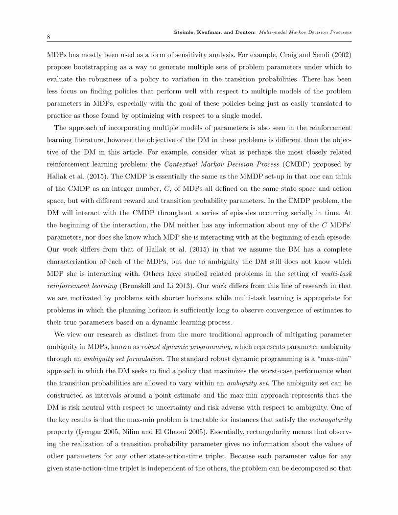
We associate any policy, π ∈Π, for the MMDP with its weighted value:
W (π) :=∑m∈M
λmvm(π) =
∑m∈M
λmEπ,Pm,µm1
[T∑t=1
rmt (st, at) + rmT+1(sT+1)
]. (3)
Thus, we consider the weighted value problem in which the goal of the DM is to find the policy
π ∈Π that maximizes the weighted value defined in (3):
Definition 2 (Weighted value problem). Given an MMDP (T ,S,A,M,Λ), the weighted
value problem is defined as the problem of finding a solution to:
W ∗ := maxπ∈Π
W (π) = maxπ∈Π
{∑m∈M
λmEπ,Pm,µm1
[T∑t=1
rmt (st, at) + rmT+1(sT+1)
]}(4)
and a set of policies Π∗ := {π∗ : W (π∗) =W ∗} ⊆Π that achieve the maximum in (4).
The weighted value problem can be viewed as an interaction between the DM (who seeks to
maximize the expected weighted value of the MMDP) and nature. In many robust formulations,
nature is viewed as an adversary which represents the risk-aversion to ambiguity in model param-
eters. However, in the weighted value problem, nature plays the role of a neutral counterpart to
the DM. In this interaction, the DM knows the complete characterization of each of the models
and nature selects which model will be given to the DM by randomly sampling according to the
probability distribution defined by Λ∈M (M). For a fixed model m∈M, there will exist an opti-
mal policy for m that is Markov (i.e., π∗m ∈ΠM). We will focus on the problem of finding a policy
that achieves the maximum in (4) when Π = ΠM . We will refer to this problem as the non-adaptive
problem because we are enforcing that the DM’s policy be based solely on the current state and she
cannot adjust her strategy based on what sequences of states she has observed. As we will show,
unlike traditional MDPs, the restriction to ΠM may not lead to an overall optimal solution. For
completeness, we will also describe an extension, called the adaptive problem, where the DM can
utilize information about the history of observed states, however this extension is not the primary
focus of this article. The evaluation of a given policy in the weighted value problem is illustrated
in Figure 1.
Steimle, Kaufman, and Denton: Multi-model Markov Decision Processes12
Figure 1 The figure illustrates the evaluation of a policy in terms of weighted value, which is the objective function
used to compare policies for an MMDP. The DM specifies a policy π which is subsequently evaluated
in each of the |M| models. The weighted value of a policy π is determined by taking of the sum of this
policy’s value in each model m, vm(π), weighted by the corresponding model weight λm.
3.1. The non-adaptive problem
The non-adaptive problem for MMDPs is an interaction between nature and the DM. In this inter-
action, the DM specifies a Markov policy, π ∈ ΠM , a priori. In this case, the policy is composed
of actions based only on the current state at each decision epoch. Therefore the policy is a distri-
bution over the actions: π = {πt(st) = (πt(1 | st), . . . , πt(|A| | st)) ∈M (A) : at ∈A, st ∈ S, t ∈ T }. In
this policy, πt(at | st) is the probability of selecting action at ∈ A if the MMDP is in state st ∈ S
at time t∈ T . Then, after the DM has specified the policy, nature randomly selects model m∈M
with probability λm. Now, nature selects s1 ∈ S according to the initial distribution µm1 ∈M (S)
and the DM selects an action, a1 ∈A, according to the pre-specified distribution π1(s1) ∈M (A).
Then, nature selects the next state s2 ∈ S according to pm1 (·|s1, a1)∈M (S). The interaction carries
on in this way where the DM selects actions according to the pre-specified policy, π, and nature
selects the next state according to the distribution given by the corresponding row of the transition
probability matrix. From this point of view, it is easy to see that under a fixed policy, the dynamics
of the stochastic process follow a Markov chain. Policy evaluation then is straightforward; one can
use backwards recursion. While policy evaluation is similar for MMDPs as compared to standard
MDPs, policy optimization is much more challenging for MMDPs. For example, value iteration,
a well-known solution technique for MDPs, does not apply to MMDPs where actions are coupled
across models.
3.2. The adaptive problem
The adaptive problem generalizes the non-adaptive problem to allow the DM to utilize realizations
of the states to adjust her strategy. In this problem, nature and the DM interact sequentially where
the DM gets new information in each decision epoch of the MMDP and the DM is allowed to utilize
the realizations of the states to infer information about the ambiguous problem parameters when

Steimle, Kaufman, and Denton: Multi-model Markov Decision Processes13
Property Non-adaptive Problem Adaptive ProblemAlways an optimalMarkov policy?
Yes Proposition 5 No Corollary 1
Always an optimaldeterministic policy?
Yes Proposition 5 Yes Corollary 2
Computational Complexity NP-hard Proposition 6 PSPACE-hard Proposition 3
Exact Solution Method MIP Proposition 7Outer linearization
with state-wise pruningProcedure 2Procedure 3
ApproximationAlgorithm
WSUMean Value Problem
Procedure 1–
– –
WSU: Bound on errorwhen |M|= 2?
Yes Proposition 10 – –
Table 1 Summary of the main properties and solution methods related to the non-adaptive and adaptive
problems for MMDPs.
selecting her future actions. In this setting, nature begins the interaction by selecting a model,
m ∈M, according to the distribution Λ, and the model selected is not known to the DM. Nature
then selects an initial state s1 ∈ S according to the model’s initial distribution, µm1 . Next, the DM
observes the state, s1, and makes her move by selecting an action, a1 ∈ A. At this point, nature
randomly samples the next state, s2 ∈ S, according to the distribution given by pm1 (·|s1, a1)∈M (S).
The interaction continues by alternating between the DM (who observes the state and selects
an action) and nature (who selects the next state according to the distribution defined by the
corresponding row of the transition probability matrix).
In the adaptive problem, the DM considers the current state of the MMDP along with informa-
tion about all previous states observed and actions taken. Because the history is available to the
DM, the DM may be able to infer which model is most likely to correctly characterize the behavior
of nature which the DM is observing. As we will formally prove later, in this context the DM will
specify a history-dependent policy in general, π= {πt(ht) : ht ∈ S ×A× . . .×A×S, t∈ T }.
4. Analysis of MMDPs
In this section, we will analyze the weighted value problem as defined in (4). For both the adaptive
and non-adaptive problems, we will describe the classes of policies that achieve the optimal weighted
value, the complexity of solving the problem, and related problems that may provide insights into
promising solution methods. These results and solution methods are summarized in Table 1. For
ease of reading, we defer all proofs to the appendix.
4.1. General properties of the weighted value problem
In both the adaptive and non-adaptive problems, nature is confined to the same set of rules.
However, the set of strategies available to the DM in the non-adaptive problem is just a subset of
the strategies available in the adaptive problem. Therefore, if W ∗N and W ∗
A are the best expected
Steimle, Kaufman, and Denton: Multi-model Markov Decision Processes14
values that the DM can achieve in the non-adaptive and adaptive problems, respectively, then it
follows that W ∗N ≤W ∗
A.
Proposition 1. W ∗N ≤W ∗
A. Moreover, the inequality may be strict.
Corollary 1. It is possible that there are no optimal policies that are Markovian for the adap-
tive problem.
The results of Proposition 1 and Corollary 1 mean that the DM may benefit from being able to
recall the history of the MMDP. This history allows for the DM to infer which model is most likely,
conditional on the observed sample path and tailor the future actions to reflect this changing belief
about nature’s choice of model. Therefore, the DM must search for policies within the history-
dependent policy class to find an optimal solution to the adaptive MMDP. These results establish
that the adaptive problem does not reduce to the non-adaptive problem in general. For this reason,
we separate the analysis for the adaptive and non-adaptive problems.
4.2. Analysis of the adaptive problem
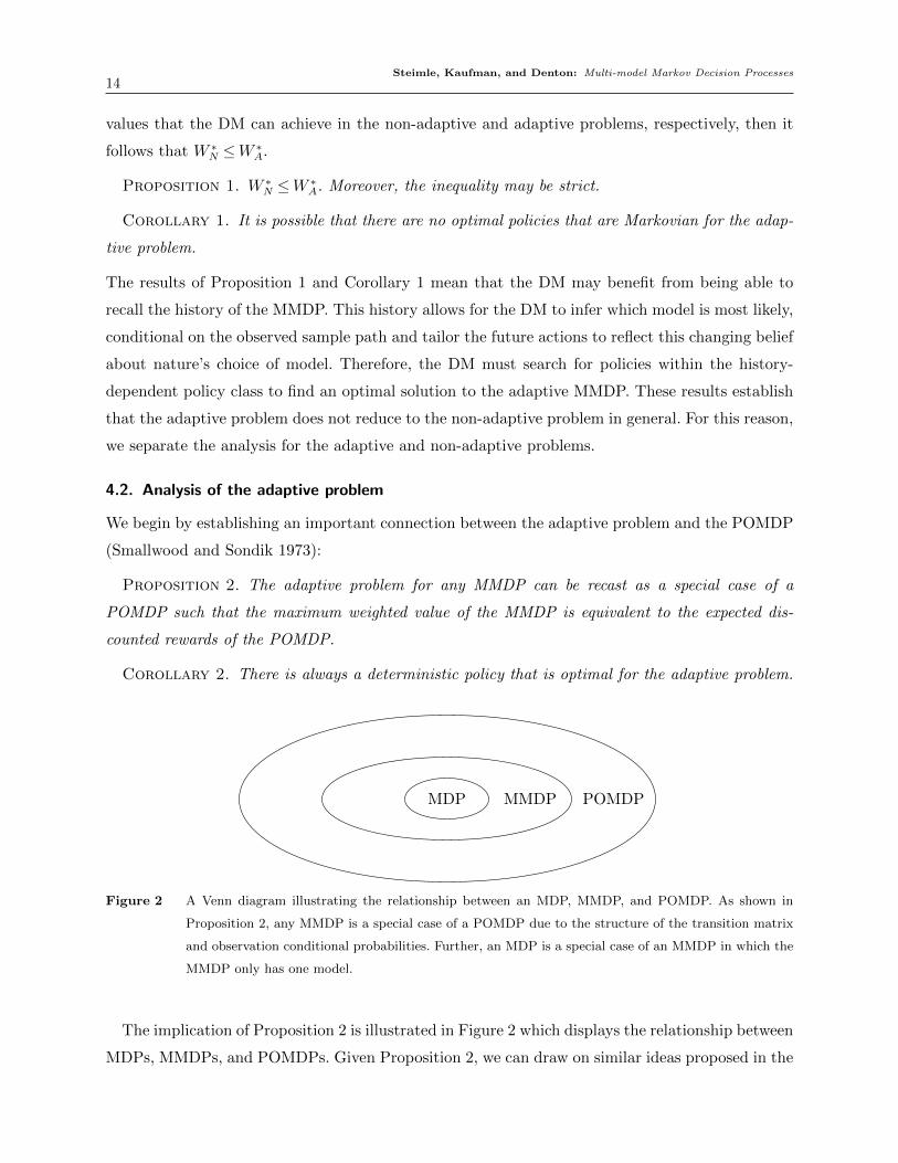
We begin by establishing an important connection between the adaptive problem and the POMDP
(Smallwood and Sondik 1973):
Proposition 2. The adaptive problem for any MMDP can be recast as a special case of a
POMDP such that the maximum weighted value of the MMDP is equivalent to the expected dis-
counted rewards of the POMDP.
Corollary 2. There is always a deterministic policy that is optimal for the adaptive problem.
MDP MMDP POMDP
Figure 2 A Venn diagram illustrating the relationship between an MDP, MMDP, and POMDP. As shown in
Proposition 2, any MMDP is a special case of a POMDP due to the structure of the transition matrix
and observation conditional probabilities. Further, an MDP is a special case of an MMDP in which the
MMDP only has one model.
The implication of Proposition 2 is illustrated in Figure 2 which displays the relationship between
MDPs, MMDPs, and POMDPs. Given Proposition 2, we can draw on similar ideas proposed in the
Steimle, Kaufman, and Denton: Multi-model Markov Decision Processes15
literature for solving POMDPs and refine them to take advantage of structural properties specific
to MMDPs. However, we show that even though MMDPs have special structure on the observation
matrix and transition probability matrix (see the proof of Proposition 2 in the appendix), we
cannot expect any improvements in the complexity of the problem due to this structure.
Proposition 3. The adaptive problem for MMDPs is PSPACE-hard.
Although the adaptive problem is PSPACE-hard and we cannot expect to develop an algorithm
whose solution time is bounded above by a function that is polynomial in the problem size, we now
discuss some special properties of the problem that can be exploited to develop an exact algorithm
for solving this problem in Section 5. We start by establishing a sufficient statistic for MMDPs:
Definition 3 (Information state for MMDPs). The information state for an MMDP is
given by a vector:
bt :=[bt(1,1), . . . , bt(S,1), bt(1,2), . . . , bt(S,2), . . . , bt(1,M), . . . , bt(S,M)
]′with elements:
bt(st,m) := P (st,m | s1, a1, . . . , st−1, at, st) .
The fact that the information state is a sufficient statistic follows directly from Proposition 2, the
formulation of a POMDP, and the special structure in the observation matrix.
Given this sufficient statistic, we establish some structural properties of the weighted value
problem:
Proposition 4. The information state, bt, has the following properties:
1. The value function is piece-wise linear and convex in the information state, bt.
2. bt(s,m)> 0⇒ bt(s′,m) = 0, ∀s′ 6= s.
3. The information state as defined above is Markovian in that the information state bt+1 depends
only on the information state and action at time t, bt and at respectively, and the state observed
at time t+1, st+1.
According to part 1, the optimal value function can be expressed as the maximum value over a
set of hyperplanes. This structural result forms the basis of our exact algorithm in Appendix B.
Part 2 states that only elements in the vector with the same value for the state portion of the
state-model pair (s,m) can be positive simultaneously, which implies that at most |M| elements
of this vector are zero. This result allows us to ignore the parts of this continuous state space that
have zero probability of being occupied. Part 3 allows for a sequential update of the belief that a
given model is the best representation of the observed states given the DM’s actions according to

Steimle, Kaufman, and Denton: Multi-model Markov Decision Processes16
Bayes’ rule. Consider the information state at time 1 at which point state s1 has been observed.
This information state can be represented by the vector with components:
b1(s,m) =
λmµ
m1 (s)∑
m′∈M λmµm′
1 (s)if s= s1,
0 otherwise.
Now, suppose that the information state at time t is bt, the DM takes action at ∈A, and observes
state st+1 at time t+ 1. Then, every component of the information state can be updated by:
bt+1(s,m) =
{Tm(bt, at, st+1) if s= st+1,
0 otherwise,
where Tm(bt, at, st+1) is a Bayesian update function that reflects the probability of model m being
the best representation of the system given the most recently observed state, the previous action,
and the previous belief state:
Tm(bt, at, st+1) :=
∑st∈S p
mt (st+1|st, at)bt(st,m)∑
m′∈M∑
st∈S pm′t (st+1|st, at)bt(st,m′)
.
As mentioned previously, our focus in this article is on applications of the MMDP framework to
medical problems in contexts for which learning by Bayesian updating is not appropriate. However,
the adaptive framework would apply to other contexts. We describe solution methods that exploit
these structural properties in Appendix B. While the methods described are likely to achieve some
degree of computational efficiency, the difficulty of solving POMDPs is such that these problems
are likely to remain intractable for all but very small model instances.
4.3. Analysis of the non-adaptive problem
In this section, we analyze the non-adaptive problem for which restricts the DM’s policy is restricted
to the class of Markov policies (ΠM). We begin by establishing the important result that there
always exists a deterministic optimal policy for the special case of the non-adaptive problem. This
result is important because searching among policies in the Markov deterministic policy class may
be appealing for several reasons: First, each individual model is solved by a policy in this class
and it could be desirable to find a policy with the same properties as the each model’s individual
optimal policy. Second, Markov policies are typically easier to implement because they only require
the current state to be stored rather than partial or complete histories of the MDP. Third, Markov
deterministic policies are ideal for medical decision making, the motivating application for this
article, because they can be easily translated to treatment guidelines that are based solely on the
information available to the physician at the time of the patient visit, such as the patient’s current
blood pressure levels. For applications in medicine, such as the case study in Section 7, deterministic
policies are a necessity since randomization is unlikely to be considered ethical outside the context
of randomized clinical trials.

Steimle, Kaufman, and Denton: Multi-model Markov Decision Processes17
Proposition 5. For the non-adaptive problem, there is always a Markov deterministic policy
that is optimal.
This result means that for the non-adaptive problem, the DM can restrict her attention to the class
of Markov deterministic policies. This result may be surprising at first due to the result of Fact 2
in Singh et al. (1994) which states that the best stationary randomized policy can be arbitrarily
better than the best stationary deterministic policy for POMDPs. While this result may seem to
contradict Proposition 5, it is worth noting that Fact 2 of Singh et al. (1994) was derived in the
context of an infinite-horizon MDP in which it is possible that the same state can be visited more
than once. In the finite-horizon MMDP, it is not possible that st could be visited more than once.
Even though the non-adaptive problem requires searching over a smaller policy class than for
the adaptive problem (ΠMD ⊂ΠHD), the non-adaptive problem is still provably hard.
Proposition 6. Solving the non-adaptive problem for an MMDP is NP-hard.
The result of Proposition 6 implies that we cannot expect to find an algorithm that solves the
non-adaptive problem for all MMDPs in polynomial time. Still, we are able to solve the non-
adaptive problem by formulating it as an MIP as discussed in the following proposition.
Proposition 7. Non-adaptive MMDPs can be formulated as the following MIP:
maxv,π
∑m∈M
λm∑s∈S
µm1 (s)vm1 (s)
s.t. vmT+1(s) ≤ rmT+1(s), ∀s∈ S,m∈M,
vmt (s) ≤ rmt (s, a) +∑s′∈S
pmt (s′|s, a)vmt+1(s′) +M(1−πt(a|s)), ∀m∈M, s∈ S, a∈A,
t∈ T ,∑a∈A
πt(a|s) = 1, ∀s∈ S, t∈ T ,
πt(a|s) ∈ {0,1}, ∀s∈ S, a∈A, t∈ T .
(5)
In this formulation, the decision variables, vmt (s)∈R, represent the value-to-go from state s∈ S
at time t∈ T in model m∈M. The binary decision variables, πt(a|s)∈ {0,1}, take on a value of 1
if the policy prescribes taking action a∈A, in state s∈ S, at epoch t∈ T , and 0 otherwise.
It is well-known that standard MDPs can be solved using a linear programming (LP) formulation
(Puterman 1994, §6.9). Suppose that vt(s, a) represents the value-to-go from state s ∈ S using
action a ∈A at decision epoch t ∈ T . The LP approach for solving MDPs utilizes a reformulation
trick that finding maxa∈A vt(s, a) is equivalent to finding minvt(s) such that vt(s) ≥ vt(s, a) for
all feasible a. In this reformulation, the constraint vt(s)≥ vt(s, a) is tight for all actions that are
optimal. The MIP formulation presented in (5) relies on similar ideas as the LP formulation of an
MDP, but is modified to enforce the constraint that the policy must be the same across all models.

Steimle, Kaufman, and Denton: Multi-model Markov Decision Processes18
In the MIP formulation of the non-adaptive MMDP, we require that constraints
vmt (s)≤ rmt (s, a) +∑s′∈S
pmt (s′|s, a)vmt+1(s′) +M(1−πt(a|s)), ∀m∈M, s∈ S, a∈A
are tight for the action a∗ ∈A such that πt(a∗|s) = 1 for any given state s∈ S, decision epoch t∈ T ,
and model m∈M. The purpose of the big-M is to ensure that vmt (s) = vmt (s, a) only if πt(a|s) = 1
meaning that the value-to-go for this state-time pair in model m ∈M corresponds to the policy
that is being used in all models. Thus, if action a ∈A is selected (and thus, πt(a|s) = 1), we want
vmt (s) = vmt (s, a) and if not (πt(a|s) = 0), we want vmt (s)≤ vmt (s, a). Therefore, we must select M
sufficiently large enough for all constraints.
The formulation of the non-adaptive problem as an MIP may seem more natural after a discussion
of the connections with two-stage stochastic programming (Birge and Louveaux 1997). If we view
the non-adaptive problem through the lens of stochastic programming, the πt(a|s) binary variables
that define the policy can be interpreted as the first-stage decisions of a two-stage stochastic
program. Moreover, nature’s choices of model, M, correspond to the possible scenarios which are
observed according to the probability distribution Λ. In this interpretation, the value function
variables, vmt (s), can be viewed as the recourse decisions. That is, once the DM has specified the
policy according to the π variables and nature has specified a model m ∈M, the DM seeks to
maximize the value function so long as it is consistent with the first-stage decisions:
V (π,m) = maxπ
[vm(π) |
∑a∈A
πt(a|s) = 1,∀s∈ S, t∈ T , πt(a|s)∈ {0,1},∀s∈ S, a∈A, t∈ T
],
where V (π) is the recourse function. This can be written as
V (π) =Em [V (π,m)] =Eπ,Pm,µm1
[T∑t=1
rt(st, at) + rT+1(sT+1)
].
The formulation in (5) is the deterministic equivalent formulation of this stochastic integer program.
Our initial numerical experiments showed that moderate-sized MDPs can be solved using (5), but
this approach may be too computationally intensive to solve large problems such as those that arise
in the context of medical decision making. This motivated the development of an approximation
algorithm that we describe in Section 5, subsequently test on randomly generated problem instances
in Section 6, and then apply to a medical decision making problem in the case study in Section 7.
The following relaxation of the non-adaptive problem allows us to quantify the performance of our
approximation algorithm:
Proposition 8. For any policy π ∈Π, the weighted value is bounded above by the weighted sum
of the optimal values in each model. That is,∑m∈M
λmvm(π)≤
∑m∈M
λm maxπ∈ΠMD
vm(π), ∀π ∈Π.
Steimle, Kaufman, and Denton: Multi-model Markov Decision Processes19
The result of Proposition 8 allows us to evaluate the performance of any MD policy even when we
cannot solve the weighted value problem exactly to determine the true optimal policy. We use this
result to illustrate the performance of our approximation algorithm in Section 7.
Proposition 8 motivates several connections between robustness and the value of information.
First, the upper bound in Proposition 8 is based on the well-known wait-and-see problem in
stochastic programming that relaxes the condition that all models must have the same policy.
Second, the expected value of perfect information (EVPI) is the expected value of the wait-and-see
solution minus the recourse problem solution:
EV PI =
[∑m∈M
λm maxπ∈ΠM
vm(π)
]− maxπ∈ΠM
[∑m∈M
λmvm(π)
].
While the wait-and-see value provides an upper bound, it may prescribe a set of solutions, one
for each model, and thus it often does not provide an implementable course of action. Another
common approach in stochastic programming is to solve the mean value problem (MVP) which
is a simpler problem in which all parameters take on their expected values. In the MMDP, this
corresponds to the case where all transition probabilities and rewards are weighted as follows:
pt(s′|s, a) =
∑m∈M
λmpmt (s′|s, a), ∀s∈ S, a∈A, t∈ T
and
rt(s, a) =∑m∈M
λmrmt (s, a).
Solving the mean value problem will give a single policy, π, which we will term the mean value
solution, with the following expected rewards:
W (π) =∑m∈M
λmvm(π).
Thus, we can create a measure of robustness for an MMDP termed the value of the weighted value
solution (VWV):
VWV =W ∗−W (π),
which parallels the well-known value of the stochastic solution (VSS) in stochastic programming
(Birge and Louveaux 1997, §4.2). If VWV is low, this implies that there is not much value from
solving the MMDP versus the MVP. On the other hand, if VWV is high, this implies that the DM
will benefit significantly from solving the MMDP.
While the non-adaptive problem has connections to stochastic programming, it also has connec-
tions to POMDPs. The non-adaptive problem can be viewed as the problem of finding the best
memoryless controller for this POMDP (Vlassis et al. 2012). Memoryless controllers for POMDPs
Steimle, Kaufman, and Denton: Multi-model Markov Decision Processes20
are defined on the most recent observation only. For an MMDP, this would translate to the DM
specifying a policy that is based only on the most recent observation of the state (recall that the DM
gets no information about the model part of the state-model pair). Because no history is allowed
to be incorporated into the definition of the policy, this policy is permissible for the non-adaptive
problem. These connections between MMDPs and stochastic programs and POMDPs allow us to
better understand the complexity and potential solution methods for finding the best solution to
the non-adaptive problem.
5. Solution methods
In this section, we will discuss how to leverage the results of Section 4 to solve the non-adaptive
problem. For conciseness, we defer the solution methods for the adaptive problem to Appendix B.
5.1. Solution methods for the non-adaptive problem
In this section, we discuss the MIP formulation of Proposition 7 for solving the non-adaptive
weighted value problem. Although the MIP formulation provides a viable way to exactly solve this
class of problems, the result of Proposition 6 motivates the need for a fast approximation algorithm
that can scale to large MMDPs.
5.1.1. Mixed-integer programming formulation The big-M constraints are an important
aspect of the MIP formulation of the weighted value problem. Thus, we discuss tightening of the
big-M values in the following constraints:
vmt (s)≤ rmt (s, a) +∑s′∈S
pmt (s′|s, a)vmt+1(s′) +M(1−πt(a|s)), ∀m∈M, s∈ S, a∈A, t∈ {1, . . . , T}.
Recall that the decision variables of the form vmt (s)∈R represent the value-to-go from state s∈ S
at time t∈ T in model m∈M under the policy specified by the x variables. For the purposes of this
discussion, we define the optimal value function for epoch t and model m for a given state-action
pair (s, a) as:
vmt (s, a) = rmt (s, a) +∑s′∈S
pmt (s′|s, a)vmt+1(s′) +M(1−πt(a|s)), ∀m∈M, s∈ S, a∈A, t∈ {1, . . . , T}.
For action a∈A, we would like the smallest value of M’s that still ensures that:
rmt (s, a) +∑s′∈S
pmt (s′|s, a)vmt+1(s′)≤ rmt (s, a′) +∑s′∈S
pmt (s′|s, a′)vmt+1(s′) +Mm,s,t, ∀a′ ∈A.
Rearranging, we obtain:
Mm,s,t ≥ rmt (s, a) +∑s′∈S
pmt (s′|s, a)vmt+1(s′)− rmt (s, a′)−∑s′∈S
pmt (s′|s, a′)vmt+1(s′), ∀a,a′ ∈A. (6)

Steimle, Kaufman, and Denton: Multi-model Markov Decision Processes21
A sufficient condition for (6) is the following:
Mm,s,t ≥maxa∈A
vmt (s, a)−mina∈A
vmt (s, a).
By the definition of vt(s, a), we are assuming that the policy defined by the x variables is being
followed after time t. However, we can relax this assumption further and allow each model to follow
a different policy to obtain the big-M values, where maxa∈A vmt (s, a) is the largest value-to-go for
this model and mina∈A vmt (s, a) is the smallest value-to-go for this model. This will provide tighter
bounds that strengthen the MIP formulation and furthermore these bounds can be computed
efficiently using standard dynamic programming methods.
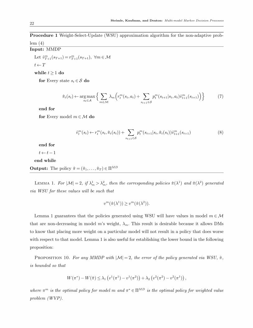
5.1.2. Weight-Select-Update (WSU) Approximation Algorithm Next, we discuss our
Weight-Select-Update (WSU) algorithm, formalized in Procedure 1, which is a fast approximation
algorithm for the non-adaptive problem. WSU generates decision rules πt ∈ΠMDt stage-wise starting
at epoch T and iterating backwards. At epoch t∈ T , the algorithm has an estimate of the value for
this policy in each model conditioned on the state st+1 at epoch t+1∈ T . This estimate is denoted
vmt+1(st+1), ∀m∈M,∀st+1 ∈ S. The algorithm weights the immediate rewards plus the value-to-go
for each of the models and then the algorithm selects, for each state, an action that maximizes
the sum of these weighted terms and denotes this action πt(st). Next, the algorithm updates the
estimated value-to-go for every state in each model according to the decision rule πt at epoch t∈ T .
This procedure iterates backwards stage-wise until the actions are specified for the first decision
epoch.
Upon first inspection, it may not be obvious that WSU is not guaranteed to produce the optimal
MD policy; however, this approximation algorithm fails to account for the fact that, under a given
policy, the likelihood of occupying a specific state could vary under the different models. The result
of Proposition 9 shows that ignoring this could lead to sub-optimal selection of actions as illustrated
in the proof.
Proposition 9. WSU is not guaranteed to produce an optimal solution to the non-adaptive
weighted value problem.
Although WSU is not guaranteed to select the optimal action for a given state-time pair, this
procedure is guaranteed to correctly evaluate the value-to-go in each model for the procedure’s
policy, π. This is because, although the action selection in equation (7) may be suboptimal, the
update of the value-to-go in each model in (8) correctly evaluates the performance of this action in
each model conditional on being in state st at decision epoch t. That is, for a fixed policy, policy
evaluation for standard MDPs applies to each of the models, separately.
Steimle, Kaufman, and Denton: Multi-model Markov Decision Processes22
Procedure 1 Weight-Select-Update (WSU) approximation algorithm for the non-adaptive prob-
lem (4)
Input: MMDP
Let vmT+1(sT+1) = rmT+1(sT+1), ∀m∈M
t← T
while t≥ 1 do
for Every state st ∈ S do
πt(st)← arg maxat∈A
{ ∑m∈M
λm
(rmt (st, at) +
∑st+1∈S
pmt (st+1|st, at)vmt+1(st+1))}
(7)
end for
for Every model m∈M do
vmt (st)← rmt (st, πt(st)) +∑
st+1∈S
pmt (st+1|st, πt(st))vmt+1(st+1) (8)
end for
t← t− 1
end while
Output: The policy π= (π1, . . . , πT )∈ΠMD
Lemma 1. For |M|= 2, if λ1m >λ
2m, then the corresponding policies π(λ1) and π(λ2) generated
via WSU for these values will be such that
vm(π(λ1))≥ vm(π(λ2)).
Lemma 1 guarantees that the policies generated using WSU will have values in model m ∈M
that are non-decreasing in model m’s weight, λm. This result is desirable because it allows DMs
to know that placing more weight on a particular model will not result in a policy that does worse
with respect to that model. Lemma 1 is also useful for establishing the lower bound in the following
proposition:
Proposition 10. For any MMDP with |M|= 2, the error of the policy generated via WSU, π,
is bounded so that
W (π∗)−W (π)≤ λ1
(v1(π1)− v1(π2)
)+λ2
(v2(π2)− v2(π1)
),
where πm is the optimal policy for model m and π∗ ∈ΠMD is the optimal policy for weighted value
problem (WVP).

Steimle, Kaufman, and Denton: Multi-model Markov Decision Processes23
Proposition 10 provides an upper bound on the error for the important special case of two
models. Unfortunately, the performance guarantee in Proposition 10 does not extend to |M|> 2.
The proof relies on Lemma 1 and the property that, when |M|= 2, λ1 = 1−λ2 to summarize the
difference between two weight vectors in terms of a single parameter which will satisfy a complete
ordering. For |M|> 2, this model-wise complete ordering is no longer available. Fortunately, the
WSU heuristic and the upper bound of Remark 8 together provide computational lower and upper
bounds, respectively.
6. Computational experiments
In this section, we describe computational experiments involving two sets of test instances for
comparing solution methods for WVP on the basis of run-time and quality of the solution. The
first set of experiments were based on a series of random instances of MMDPs. The second set
of experiments was based on a small MDP for determining the most cost-effective HIV treatment
policy which has been used for pedagogical purposes in the medical decision making literature
(Chen et al. 2017).
To compare the solution methods, we will generate a solution for each instance using the WSU
heuristic, mean value problem (MVP) heuristic, and the MIP formulation. We will compare the
weighted value policies obtained via the heuristics (WN(π)) to the optimal value obtained by solving
the MIP to within 1% of optimality, W ∗N :
Gap =W ∗N −WN(π)
W ∗N
× 100%,
where π is the policy obtained from either WSU or MVP. WSU and MVP were implemented using
Python 3.7. All MIPs were solved using Gurobi 8.1.1.
6.1. Test instances
We now describe the two sets of test instances used to compare the solution methods.
6.1.1. Random instances To generate the random test instances, first, the number of states,
actions, models, and decision epochs for the problem were defined. Then, model parameters were
randomly sampled. In all test instances, it was assumed that the sampled rewards were the same
across models, the weights were uninformed priors on the models, and the initial distribution was
a discrete uniform distribution across the states. The rewards were sampled from the uniform dis-
tribution: r(s, a)∼U(0,1),∀(s, a)∈ S ×A. The transition probabilities were obtained by sampling
from a Dirichlet distribution (Dir), which has a set of parameters defining a base measure and
a parameter defining the concentration of the distribution. For each row, the base measure was
determined by sampling a uniform U(0,1) for each possible transition: p(s′|s, a)∼ U(0,1). Then,

Steimle, Kaufman, and Denton: Multi-model Markov Decision Processes24
for every (m,s,a, s′)∈M×S×A×S, the transition probabilities were normalized so that the row
of the transition probability matrix had elements that sum to one:
p(s′|s, a) :=p(s′|s, a)∑
s′′∈S p(s′′|s, a)
.
The p(s′|s, a) values are then used as the base measure for the Dirichlet distribution, and we
vary the concentration parameter to control for the amount of variation among the models to
control for the amount of variance among the models. Dirichlet distributions with the same base
measure will have the same mean value of the transition row, but higher values of the concentration
parameter correspond to distributions with less variance. For each sample, we scale by a factor of
β ∝mins′∈S p(s′|s, a) for β = 1, 10, and 100:
(pm(1|s, a), . . . , pm(|S||s, a))∼Dir(βp(1|s, a), . . . , βp(|S||s, a))∀s∈ S, a∈A,m∈M.
These experiments allow us to test the performance of the solution methods on many different
kinds of MMDPs, however these instances are not guaranteed to have structured transitions and
rewards that one might expect in practice. Therefore, we also include the following test instances
that has a structure commonly observed in MDPs for medical decision making.
6.1.2. Medical decision making instances We also consider a second set of test instances
which matches the medical decision making context of our case study. The example we consider
has been used many times in the medical decision making literature for illustrative purposes to
demonstrate various methods.
In this set of experiments, we consider an MDP for determining the optimal timing of treatments
for HIV. In the MDP, HIV is characterized according to 4 health states: Mild, Moderate, Severe,
or Dead. The patient transitions from the less severe states to the more severe states according to
a Markov chain. The DM can choose to start the patient on one of three treatments: Treatment
A, Treatment B, and Treatment C. Treatment A is the least effective but also the least expensive
while Treatment C is the most effective but comes at the highest cost. Chen et al. (2017) provides
a summary table of parameter values for this MDP as well as some sampling distributions for
each parameter. In our experiments, we construct an MMDP by sampling parameters from the
corresponding distributions. We consider 10, 20, and 30 models in the MMDP and vary the number
of decision epochs from 5 to 10 to explore how the proposed methods perform.
6.2. Results
We now present the results of our computational experiments comparing solution methods for
WVP for these two sets of test instances.
Steimle, Kaufman, and Denton: Multi-model Markov Decision Processes25
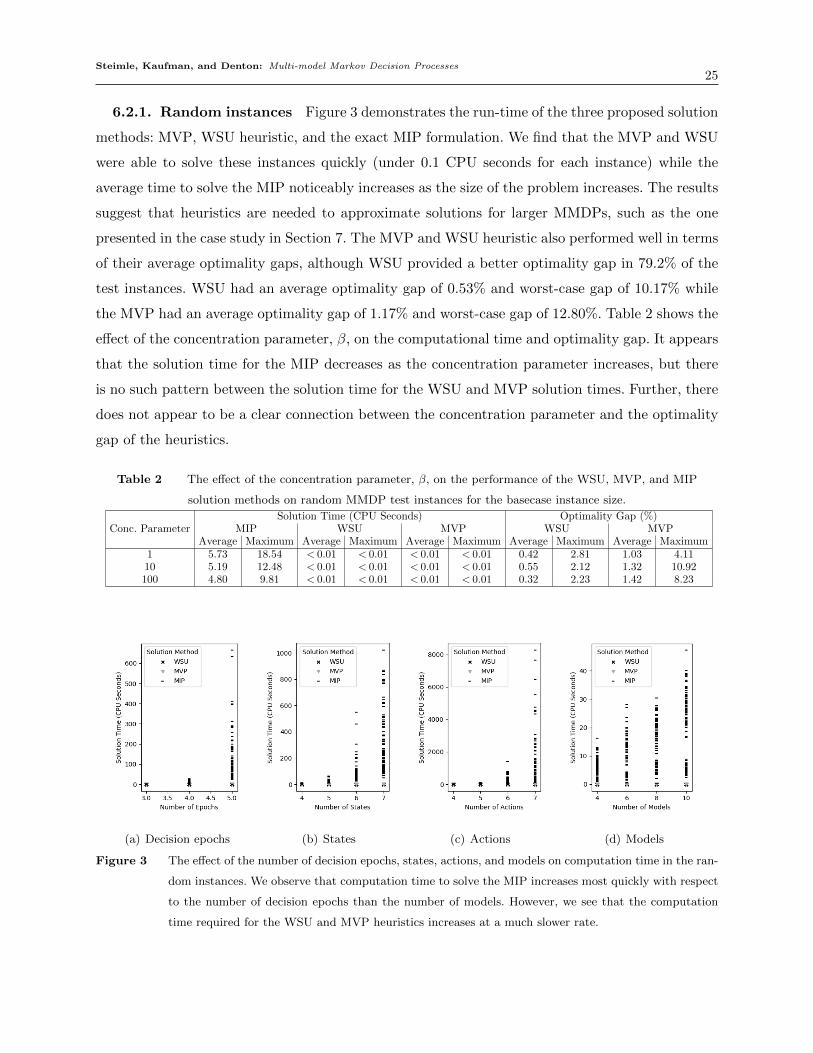
6.2.1. Random instances Figure 3 demonstrates the run-time of the three proposed solution
methods: MVP, WSU heuristic, and the exact MIP formulation. We find that the MVP and WSU
were able to solve these instances quickly (under 0.1 CPU seconds for each instance) while the
average time to solve the MIP noticeably increases as the size of the problem increases. The results
suggest that heuristics are needed to approximate solutions for larger MMDPs, such as the one
presented in the case study in Section 7. The MVP and WSU heuristic also performed well in terms
of their average optimality gaps, although WSU provided a better optimality gap in 79.2% of the
test instances. WSU had an average optimality gap of 0.53% and worst-case gap of 10.17% while
the MVP had an average optimality gap of 1.17% and worst-case gap of 12.80%. Table 2 shows the
effect of the concentration parameter, β, on the computational time and optimality gap. It appears
that the solution time for the MIP decreases as the concentration parameter increases, but there
is no such pattern between the solution time for the WSU and MVP solution times. Further, there
does not appear to be a clear connection between the concentration parameter and the optimality
gap of the heuristics.
Table 2 The effect of the concentration parameter, β, on the performance of the WSU, MVP, and MIP
solution methods on random MMDP test instances for the basecase instance size.
Conc. ParameterSolution Time (CPU Seconds) Optimality Gap (%)
MIP WSU MVP WSU MVPAverage Maximum Average Maximum Average Maximum Average Maximum Average Maximum
1 5.73 18.54 < 0.01 < 0.01 < 0.01 < 0.01 0.42 2.81 1.03 4.1110 5.19 12.48 < 0.01 < 0.01 < 0.01 < 0.01 0.55 2.12 1.32 10.92100 4.80 9.81 < 0.01 < 0.01 < 0.01 < 0.01 0.32 2.23 1.42 8.23
(a) Decision epochs (b) States (c) Actions (d) Models
Figure 3 The effect of the number of decision epochs, states, actions, and models on computation time in the ran-
dom instances. We observe that computation time to solve the MIP increases most quickly with respect
to the number of decision epochs than the number of models. However, we see that the computation
time required for the WSU and MVP heuristics increases at a much slower rate.

Steimle, Kaufman, and Denton: Multi-model Markov Decision Processes26
(a) Computation time vs. number of decision epochs (b) Computation time vs. number of models
Figure 4 The effect of the number of decision epochs and number of models on computation time in the medical
decision making instances. We observe that computation time to solve the MIP increases more quickly
with respect to the number of decision epochs than the number of models. However, we see that the
computation time required for the WSU and MVP heuristics increases at a much slower rate.
6.2.2. Medical decision making instances Figure 4 demonstrates the run-time of the three
proposed solution methods on the medical decision making instances. We find that the MVP and
WSU were able to solve these instances relatively quickly (under 0.1 CPU seconds for each instance)
while the average time to solve the MIP noticeably increases as the size of the number of decision
epochs increases (from 1.73 CPU seconds on average for 4 decision epochs to 141.84 CPU seconds
for 6 decision epochs). For the instances with 6 decision epochs, the MIP computation time rose
from 21.73 CPU seconds on average for 5 models to 111.04 CPU seconds for 15 models. Comparing
WSU and MVP in terms of optimality gap, we observe that for these test instances, both WSU
and MVP perform quite well with maximum optimality gaps under 0.45% and 0.69% respectively.
These results suggest that the MVP and WSU heuristics may be suitable for generating solutions to
medical decision making instances. The case study in Section 7 considers a larger medical decision
making problem in the context of preventive blood pressure and cholesterol management.
7. Case study: blood pressure and cholesterol management in type 2 diabetes
In this section, we present an MMDP to optimize the timing and sequencing of the initiation of
blood pressure medications and cholesterol medications for patients with type 2 diabetes. A non-
adaptive MMDP is appropriate for this case study because the goal is to design treatment guidelines
to prevent cardiovascular events. Thus, adaptive learning cannot be used to resolve the underlying
source of ambiguity (models for the risk of events) without exposing patients to heightened risk of
events. Something that would be considered unethical in the context of preventive medicine. Here,

Steimle, Kaufman, and Denton: Multi-model Markov Decision Processes27
WSU was used to generate a policy that trades off conflicting estimates of cardiovascular risk from
two well-established studies in the medical literature. We begin by providing some context about
the problem, the MMDP model, and the parameter ambiguity that motivates its use.
Diabetes is one of the most common and costly chronic medical conditions, affecting more than
25 million adults, or 11% of the adult population in the United States (CDC 2011). Diabetes
is associated with the inability to properly metabolize blood glucose (blood sugar) and other
metabolic risk factors that place the patient at risk of complications including coronary heart
disease (CHD) and stroke. There are several types of diabetes including type 1 diabetes, in which
the patient is dependent on insulin to live, gestational diabetes, which is associated with pregnancy,
and type 2 diabetes in which the patient has some ability (albeit impaired) to manage glucose. In
this case study we focus on type 2 diabetes, which accounts for more than 90% of all cases.
The first goal, glycemic control, is typically achieved quickly following diagnosis of diabetes using
oral medications and/or insulin. Management of cardiovascular risk, the focus of this case study,
is a longer term challenge with a complex tradeoff between the harms of medication and the risk
of future CHD and stroke events. Patients with diabetes are at much higher risk of stroke and
CHD events than the general population. Well-known risk factors include total cholesterol (TC),
high density lipids (HDL – often referred to as “good cholesterol”), and systolic blood pressure
(SBP). Like blood glucose, the risk factors of TC, HDL, and BP are also controllable with medical
treatment. Medications, such as statins and fibrates, can reduce TC and increase HDL. Similarly,
there are a number of medications that can be used to reduce blood pressure including ACE
inhibitors, ARBs, beta blockers, thiazide, and calcium channel blockers. All of these medications
have side effects that must be weighed against the long-term benefits of lower risk of CHD and
stroke. An added challenge to deciding when and in what sequence to initiate medication is due
to the conflicting risk estimates provided by two well known clinical studies: the FHS (Wolf et al.
1991, Wilson et al. 1998) and the ACC/AHA assessment of cardiovascular risk (Goff et al. 2014).
7.1. MMDP formulation
The MDP formulation of Mason et al. (2014) was adapted to create an MMDP based on the FHS
risk model (Wolf et al. 1991, Wilson et al. 1998) and the ACC/AHA risk model (Goff et al. 2014).
These are the most well-known risk models used by physicians in practice. The state space of
the MMDP is a finite set of health states defined by SBP, TC, HDL, and current medications. A
discrete set of actions represent the initiation of the two cholesterol medications and 4 classes of
blood pressure medications. The objective is to optimize the timing and sequencing of medication
initiation to maximize quality-adjusted life years (QALYs). QALYs are a common measure used
to assess health interventions that account for both the length of a patient’s life as well as the loss
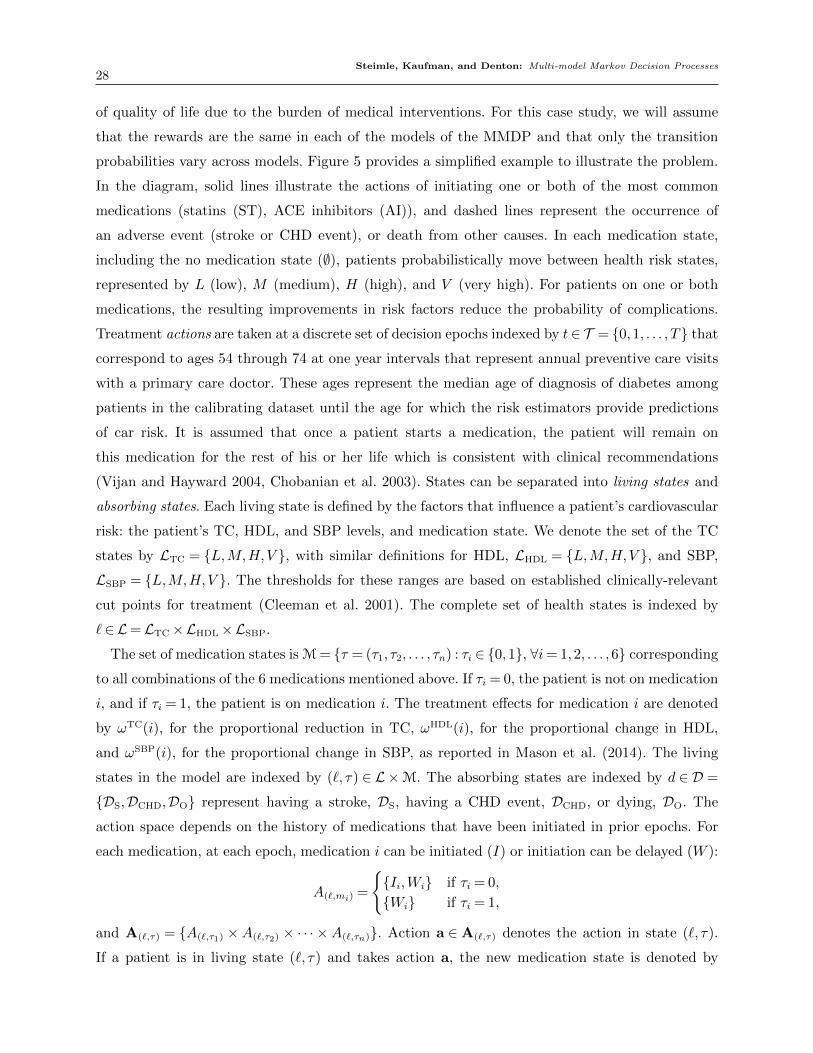
Steimle, Kaufman, and Denton: Multi-model Markov Decision Processes28
of quality of life due to the burden of medical interventions. For this case study, we will assume
that the rewards are the same in each of the models of the MMDP and that only the transition
probabilities vary across models. Figure 5 provides a simplified example to illustrate the problem.
In the diagram, solid lines illustrate the actions of initiating one or both of the most common
medications (statins (ST), ACE inhibitors (AI)), and dashed lines represent the occurrence of
an adverse event (stroke or CHD event), or death from other causes. In each medication state,
including the no medication state (∅), patients probabilistically move between health risk states,
represented by L (low), M (medium), H (high), and V (very high). For patients on one or both
medications, the resulting improvements in risk factors reduce the probability of complications.
Treatment actions are taken at a discrete set of decision epochs indexed by t∈ T = {0,1, . . . , T} that
correspond to ages 54 through 74 at one year intervals that represent annual preventive care visits
with a primary care doctor. These ages represent the median age of diagnosis of diabetes among
patients in the calibrating dataset until the age for which the risk estimators provide predictions
of car risk. It is assumed that once a patient starts a medication, the patient will remain on
this medication for the rest of his or her life which is consistent with clinical recommendations
(Vijan and Hayward 2004, Chobanian et al. 2003). States can be separated into living states and
absorbing states. Each living state is defined by the factors that influence a patient’s cardiovascular
risk: the patient’s TC, HDL, and SBP levels, and medication state. We denote the set of the TC
states by LTC = {L,M,H,V }, with similar definitions for HDL, LHDL = {L,M,H,V }, and SBP,
LSBP = {L,M,H,V }. The thresholds for these ranges are based on established clinically-relevant
cut points for treatment (Cleeman et al. 2001). The complete set of health states is indexed by
`∈L=LTC×LHDL×LSBP.
The set of medication states is M= {τ = (τ1, τ2, . . . , τn) : τi ∈ {0,1}, ∀i= 1,2, . . . ,6} corresponding
to all combinations of the 6 medications mentioned above. If τi = 0, the patient is not on medication
i, and if τi = 1, the patient is on medication i. The treatment effects for medication i are denoted
by ωTC(i), for the proportional reduction in TC, ωHDL(i), for the proportional change in HDL,
and ωSBP(i), for the proportional change in SBP, as reported in Mason et al. (2014). The living
states in the model are indexed by (`, τ) ∈ L×M. The absorbing states are indexed by d ∈ D =
{DS,DCHD,DO} represent having a stroke, DS, having a CHD event, DCHD, or dying, DO. The
action space depends on the history of medications that have been initiated in prior epochs. For
each medication, at each epoch, medication i can be initiated (I) or initiation can be delayed (W ):
A(`,mi) =
{{Ii,Wi} if τi = 0,
{Wi} if τi = 1,
and A(`,τ) = {A(`,τ1) ×A(`,τ2) × · · · ×A(`,τn)}. Action a ∈A(`,τ) denotes the action in state (`, τ).
If a patient is in living state (`, τ) and takes action a, the new medication state is denoted by

Steimle, Kaufman, and Denton: Multi-model Markov Decision Processes29
Figure 5 An illustration of the state and action spaces of the MDP as illustrated in Mason et al. (2014). In
the corresponding MMDP, when medications are initiated (solid lines denote actions), the risk factors
are improved and the probability of an adverse event (denoted by the dashed lines) is reduced. The
probabilities of adverse events may differ in the different models depending on the risk calculator that
was used to estimate the probability.
τ ′, where τ ′i is set to 1 for any medications i that are newly initiated by action a; τ ′i = τi for all
medications i which are not newly initiated. Once medication i is initiated, the associated risk
factor is modified by the medication effects denoted by ωTC(i), ωHDL(i), and ωSBP(i), resulting in
a reduction in the probability of a stroke or CHD event. Two types of transition probabilities are
incorporated into the model: probabilities of transition among health states and the probability
of events (fatal and nonfatal). At epoch t, pτt (d|`) denotes the probability of transition from state
(`, τ) ∈ L ×M to an absorbing state d ∈ D. Given that the patient is in health state ` ∈ L, the
probability of being in health state `′ in the next epoch is denoted by qt(`′|`). The health state
transition probabilities, qt(`′|`), were computed from empirical data for the natural progression of
BP and cholesterol adjusted for the absence of medication (Denton et al. 2009). We define pτt (j|`)
to be the probability of a patient being in state j ∈ L∪D at epoch t+ 1, given the patient is in
living state (`, τ) at epoch t. The transition probabilities can be written as:
pτt (j|i) =
[1−
∑d∈D
pτt (d|i)]qt(j|i) if i, j ∈L,
pτt (j|i) if i∈L, j ∈D,
1 if i= j ∈D,
0 otherwise.
The two models of the MMDP represent the different cardiovascular risk calculators used to esti-
mate the transition probabilities to the absorbing states: pτt (d|i) for i ∈ L, d ∈ D. We will refer to
the model using the ACC/AHA study as model A and the model using FHS as model F . We weight

Steimle, Kaufman, and Denton: Multi-model Markov Decision Processes30
these models by λA ∈ [0,1] and λF := 1−λA respectively. We estimate of all other cause mortality
based take from the Centers for Disease Control and Prevention life tables (Arias et al. 2011). The
reward rt(`, τ) for a patient in health state ` at epoch t is:
rt(`, τ) =Q(`, τ),
where Q(`, τ) = 1 − dMED(τ) is the reward for one QALY. QALYs are elicited through patient
surveys, and are commonly used for health policy studies (Gold et al. 2002). The disutility factor,
dMED(τ), represents the estimated decrease in quality of life due to the side effects associated with
the medications in τ . We use the disutility estimates provided in Mason et al. (2014).
The goal of this case study is to design treatment guidelines that maximize population-level out-
comes. For this reason, the non-adaptive problem is more appropriate because it designs guidelines
that could be recommended to an entire population of patients. In contrast, a personalized medicine
approach might try to infer whether ACC/AHA or Framingham is the “representative risk model”
for an individual patient and might motivate the use of the adaptive framework. However, this is
not the focus of this case study.
7.2. Results
Using the MMDP described above, we evaluated the performance of the solutions generated via
WSU in terms of computation time and the objective function of QALYs until first event. We also
discuss the policy associated with the solution generated using WSU when the weights are treated
as an uninformed prior on the models. The MMDP had 4099 states, 64 actions, 20 decision epochs,
and 2 models.
Table 3 Time to approximate a solution to the weighted problem using the Weight-Select-Update (WSU)
algorithm and to solve each of the nominal models using standard dynamic programming, in CPU seconds.
Female MaleWSU with λF = λA = 0.5 10.98 sec. 11.08 sec.Standard DP, FHS Model 8.70 sec. 8.77 sec.Standard DP, ACC/AHA Model 8.98 sec. 9.00 sec.
Table 3 shows the computation time required to run WSU with λF = λA = 0.5, as well as
the time required to solve the FHS model and the ACC/AHA model using standard dynamic
programming, for the female and male problem parameters. While WSU requires more computation
time than standard dynamic programming for each of the individual models, WSU does not take
more computation time than the total time for solving both of the nominal models.
Figure 6 shows the performance of the policies generated using WSU when evaluated in the
ACC/AHA and FHS models, as well as the weighted value of these two models for the corresponding

Steimle, Kaufman, and Denton: Multi-model Markov Decision Processes31
●
●●
●
●
●
●
●
●
●
●
●
●
●
●
●
●
●
●
●
●
●
●
●
●
●
●
●
●
●
●
●
●
●
●
●
●
●
●
●
●
●
●
●
●
●
●
●
●
●
●
●
●
●
●
●
●
●
●
●
●●
●14,300
14,400
14,500
14,600
14,700
14,800
0 25 50 75 100Weight on FHS in Weight−Select−Update, (%)
QA
LYs
Per
100
0 M
en
Evaluation Metric●
●
●
ACC/AHA QALYs, vA (π)FHS QALYs, vF (π)
Weighted QALYs, W(π)
(a) Male
●
●●
●
●
●
●
●
●
●
●
●
●
●
●
●
●
●
●
●
●
●
●
●
●
●
●
●
●
●
●
●
●
●
●
●
●
●
●
●
●
●
●
●
●
●
●
●
●
●
●
●
●
●
●
●
●
●●
●
●●
●
15,250
15,500
15,750
16,000
16,250
0 25 50 75 100Weight on FHS in Weight−Select−Update, (%)
QA
LYs
Per
100
0 W
omen
Evaluation Metric●
●
●
ACC/AHA QALYs, vA (π)FHS QALYs, vF (π)
Weighted QALYs, W(π)
(b) Female
Figure 6 The performance of the policies generated using the Weight-Select-Update (WSU) approximation algo-
rithm for the MMDP for treatment of men (Figure 6a) and women (Figure 6b). For each choice of the
weight on the FHS model in WSU, the graph shows the performance of these policies with respect to
three different metrics: the performance in the ACC/AHA model (light grey), the performance in the
FHS model (dark grey), and the weighted value (black). The dashed line represents the upper bound
from Proposition 8.

Steimle, Kaufman, and Denton: Multi-model Markov Decision Processes32
choice of the weight on the FHS model, λF . The dashed line in these figures represents the upper
bound from Proposition 8. When λF = 100%, WSU finds the optimal policy for the FHS model
which is why the maximum the FHS value is achieved at λF = 100%. Of the WSU policies, the
worst value in the ACC/AHA model is achieved at this point because the algorithm ignores the
performance in the ACC/AHA model. Analogously, when λF = 0%, WSU finds the optimal policy
for the ACC/AHA model which is why the performance in the ACC/AHA model achieves its
maximum and the performance in the FHS model is at its lowest value at this point. For values
of λF ∈ (0,1), WSU generates policies that trade-off the performance between these two models.
We found that WSU generated policies that slightly outperformed the policy generated by solving
the MVP. As supported by Proposition 1, WSU has the desirable property that the performance
in model m is non-decreasing in λm. For women, using the FHS model’s optimal policy leads to
a severe degradation in performance with respect to the ACC/AHA model. In contrast, WSU is
able to generate policies that do not sacrifice too much performance in the ACC/AHA model in
order to improve performance in the FHS model. The results for women clearly illustrate why
taking a max-min approach instead of the MMDP approach can be problematic in some cases. To
see this, note that the FHS model’s optimal policy is a solution to the max-min problem because
vF (π∗F )< vA(π∗F ) and thus no policy will be able to achieve a better value than π∗F in the FHS model.
However, Figure 6(b) shows that this policy leads to a significant degradation in performance in
the ACC/AHA model relative to that model’s optimal policy π∗A. This demonstrates why taking a
max-min approach, which is common in the robust MDP literature as pointed out in Section 2, can
have the unintended consequence of ignoring the performance of a policy in all but one model in
some cases. By taking the weighted value approach with nontrivial weights on the models, the DM
is forced to consider the performance in all models. By generating policies using WSU by varying
λF ∈ (0,1), the DM can strike a balance between the performance in the ACC/AHA model and
the FHS model.
Table 4 illustrates that the WSU approximation algorithm generates a policy that will perform
well in both the ACC/AHA model and in the FHS model. The table reports the QALYs gained per
1000 persons relative to a benchmark policy of never initiating treatment; these values are reported
for three policies: (1) the ACC/AHA model’s optimal policy, (2) the FHS model’s optimal policy,
and (3) the WSU policy. While using a model’s optimal policy results in the highest possible QALY
gain in that model, that model’s optimal policy can sacrifice performance when evaluated in the
other model. This is illustrated in the table in terms of regret ; regret for a specific model is defined
to be the difference between the QALYs gained by that model’s optimal policy and the QALYs
gained by the specified policy. The table shows that in the ACC/AHA model, the FHS model’s
optimal policy achieves 134.4 QALYs per 1000 men less than the ACC/AHA model’s optimal

Steimle, Kaufman, and Denton: Multi-model Markov Decision Processes33
(a) Male
Metric(per 1000 men)
EvaluationACC/AHA
Optimal PolicyFHS
Optimal PolicyWSUPolicy
QALYs GainedOver No Treatment
ACC/AHA 695.9 561.5 679.3FHS 1788.9 1880.5 1841.4Weighted 1242.4 1211.0 1260.4
RegretACC/AHA 0 134.4 16.6FHS 91.6 0 39.1Weighted 45.8 67.2 27.9
(b) Female
Metric(per 1000 women)
EvaluationACC/AHA
Optimal PolicyFHS
Optimal PolicyWSUPolicy
QALYS GainedOver No Treatment
ACC/AHA 205.2 −155.3 147.9FHS 1401.1 1670.4 1464.1Weighted 803.1 757.5 806.0
RegretACC/AHA 0 360.5 57.3FHS 269.3 0 206.3Weighted 134.7 180.2 131.8
Table 4 The performance of 3 policies in terms of QALYs gained over no treatment and regret for (a) men and
(b) women. The 3 policies are (1) the optimal policy for the ACC/AHA model, (2) the optimal policy for the FHS
model, and (3) the policy generated via the Weight-Select-Update (WSU) approximation algorithm which considers
both the ACC/AHA and FHS models simultaneously. These policies are evaluated in terms of the QALYs gained
over a policy which never initiates medication in the ACC/AHA model and the FHS model, as well as the weighted
QALYs gained over no treatment in these two models. Regret is determined by taking the difference between the
QALYs obtained by the optimal policy for a model and the QALYs obtained by the given policy.
policy while the WSU policy is able to achieve only 16.6 less QALYs per 1000 men. Similarly, in
the FHS model, the ACC/AHA model’s optimal policy sacrifices 91.6 fewer QALYs per 1000 men
relative to the optimal policy for the ACC/AHA model while the WSU policy only sacrifices 39.1
QALYs per 1000 men relative to the optimal policy for this model. Assuming an uninformed prior,
the WSU approximation algorithm with equal weights on the models provides a weighted regret
that is 17.9 and 2.9 QALYs less than the ACC/AHA model’s optimal policy for men and women
respectively, and WSU achieved a weighted regret that was 39.3 and 48.4 QALYs less than the
FHS models’ optimal policy for men and women respectively. For women in particular, we find
that using ignoring ambiguity in the risk calculations could potentially lead to very poor outcomes.
The findings suggest that the FHS model’s optimal policy is worse than the no treatment policy in
the ACC/AHA model results. This is likely because the FHS model’s optimal policy is much more
aggressive in terms of starting medications (as seen in Figure 7, which is discussed later). Therefore,
it seems that the FHS model’s optimal policy is starting many women on medication which leads
them to incur the disutility associated with these medications, but that these medications do not
provide much benefit in terms of risk reduction in the ACC/AHA model. While the ACC/AHA
model’s optimal policy outperforms the no treatment policy in the Framingham model, we still

Steimle, Kaufman, and Denton: Multi-model Markov Decision Processes34
see a large amount of regret in terms of QALYs gained per 1000 women in the FHS model. For
both of these models, the WSU policy finds a policy that achieves a lower regret than the “other”
model’s optimal policy. Once again, weighting the regret from the two models equally, we see that
the WSU policy is able to hedge against the ambiguity in risk for women and outperforms the two
policies which ignore ambiguity.
It is interesting to note that the regret achieved by the WSU is much smaller for men than for
women. This may be due to the disparity in the effects of ambiguity on decision making for women
and men. EVPI is one way to quantify the expected value of resolving ambiguity and gives a DM a
sense of how valuable it would be to obtain better information. Because WSU ≤W ∗, the following
is an upper bound on EV PI: EV PI =WS −W ∗ ≤WS −WSU . For this case study, the upper
bound on the EVPI suggests that as many as 28 QALYs per 1000 men and 131.8 QALYs per 1000
women could be saved if there were no ambiguity in the cardiovascular risk of the patient. Estimates
such as this provide insight into the value of future studies that could reduce the ambiguity.
Figures 7(a) and 7(b) illustrate medication use for male and female patients, respectively, under
three different policies: the ACC/AHA model’s optimal policy, the FHS model’s optimal policy,
and a policy generated via WSU with λF = λA = 50%. These figures illustrate the probability that
a patient who follows the specified policy from age 54 will be on the corresponding medication,
conditioned on the patient being alive, as a function of their age. For men, the optimal policy for
FHS model and the optimal policy for the ACC/AHA model agree that all men should start statins
immediately, which could be explained by the relatively low disutility and high risk reduction of
statins in both models. However, the models disagree in the use of fibrates and the 4 classes of blood
pressure medications. The optimal policy for the ACC/AHA model suggests that all men should
start fibrates immediately, suggesting that cholesterol control is important in the ACC/AHA model.
However, fibrates are less commonly prescribed under the FHS model’s optimal policy with about
two-thirds of men on this medication by age 65. The policy generated with WSU agrees with the
ACC/AHA policy’s more extensive use of fibrates which may suggest that focusing on cholesterol
control could be a good strategy in both models. Among the blood pressure medications, there are
some disagreements between the optimal policies of the two models, with the most distinct being
for the use of calcium channel blockers. This is likely to be due to the relatively high disutility (from
side effects of calcium channel blockers) and low risk reduction associated with this medication.
In the ACC/AHA model, the risk reduction of calcium channel blockers is worth the disutility
in many cases, but in the FHS model, there are few instances in which the disutility associated
with this medication is worth the gain in QALYs. The policy generated with WSU generates a
policy that strikes a balance between these two extremes. While the differences are not quite as
extreme, WSU also generates a policy that balances the utilization of thiazides prescribed by each

Steimle, Kaufman, and Denton: Multi-model Markov Decision Processes35
●
● ● ● ● ● ● ● ● ● ● ● ● ● ● ● ● ● ● ●
●
● ● ● ● ● ● ● ● ● ● ● ● ● ● ● ● ● ● ●
●
● ● ● ● ● ● ● ● ● ● ● ● ● ● ● ● ● ● ●
0
25
50
75
100
55 60 65 70Age
Med
icat
ion
Use
(%
)
Statins
●
● ● ● ● ● ● ● ● ● ● ● ● ● ● ● ● ● ● ●
●
● ● ● ● ● ● ● ● ● ● ● ● ● ● ● ● ● ● ●
●
●
●
●●
●● ● ● ● ● ● ●
● ● ● ● ● ● ●
0
25
50
75
100
55 60 65 70Age
Med
icat
ion
Use
(%
)
Fibrates
●
●
●
●
●
●●
●●
● ● ● ● ● ● ● ● ● ● ●
●
●
●
●
●●
● ● ● ● ● ● ● ● ● ● ● ● ● ●
●
●
●●
● ● ● ● ● ● ● ● ● ● ● ● ● ● ● ●
0
25
50
75
100
55 60 65 70Age
Med
icat
ion
Use
(%
)
Beta Blockers
●
●
●
●
●
●●
●●
● ● ● ● ● ● ● ● ● ● ●
●
●
●
●
●●
● ● ● ● ● ● ● ● ● ● ● ● ● ●
●
●
●
●
●●
●●
● ● ● ● ● ● ● ● ● ● ● ●
0
25
50
75
100
55 60 65 70Age
Med
icat
ion
Use
(%
)
Thiazides
●
●
●
●
●
●●
●●
● ● ● ● ● ● ● ● ● ● ●
●
●
●
●
●●
● ● ● ● ● ● ● ● ● ● ● ● ● ●
●
●
●
●
●●
●●
●● ● ● ● ● ● ● ● ● ● ●
0
25
50
75
100
55 60 65 70Age
Med
icat
ion
Use
(%
)
ACE/ARB
●
●
●
●
●
●●
●●
● ● ● ● ● ● ● ● ● ● ●
●
●
●
●
●
●
●
●
●
●●
●● ● ● ● ● ● ● ●
● ●
● ● ● ● ● ● ● ● ● ● ● ● ● ● ● ● ● ●
0
25
50
75
100
55 60 65 70Age
Med
icat
ion
Use
(%
)
Calcium Channel Blockers
Policy ● ● ●ACC/AHA Optimal Policy Framingham Optimal Policy Weight−Select−Update with λF = λA = 50%
(a) Male
●
● ● ● ● ● ● ● ● ● ● ● ● ● ● ● ● ● ● ●
●
● ● ● ● ● ● ● ● ● ● ● ● ● ● ● ● ● ● ●
●
● ● ● ● ● ● ● ● ● ● ● ● ● ● ● ● ● ● ●
0
25
50
75
100
55 60 65 70Age
Med
icat
ion
Use
(%
)
Statins
●
● ● ● ● ● ● ● ● ● ● ● ● ● ● ● ● ● ● ●
●
●
●
● ●● ● ● ● ● ● ● ● ● ● ● ● ● ● ●
●
●
●
● ●
●● ●
● ● ● ● ●● ● ● ● ● ● ●
0
25
50
75
100
55 60 65 70Age
Med
icat
ion
Use
(%
)
Fibrates
● ● ● ● ● ● ● ● ● ● ● ● ● ● ● ● ● ● ● ●●
●● ● ● ● ● ● ● ● ● ● ● ● ● ● ● ● ● ●
●
●●
● ● ● ● ● ● ● ● ● ● ● ● ● ● ● ● ●
0
25
50
75
100
55 60 65 70Age
Med
icat
ion
Use
(%
)
Beta Blockers
● ● ● ● ● ● ● ● ● ● ● ● ● ● ● ● ● ● ● ●●
●● ● ● ● ● ● ● ● ● ● ● ● ● ● ● ● ● ●
●
●
●
●● ● ● ● ● ● ● ● ● ● ● ● ● ● ● ●
0
25
50
75
100
55 60 65 70Age
Med
icat
ion
Use
(%
)
Thiazides
● ● ● ● ● ● ● ● ● ● ● ● ● ● ● ● ● ● ● ●● ●● ● ● ● ● ● ● ● ●
●
● ● ● ● ● ● ● ●
● ● ● ● ● ● ● ● ● ● ● ● ● ● ● ● ● ●
● ●
0
25
50
75
100
55 60 65 70Age
Med
icat
ion
Use
(%
)
ACE/ARB
● ● ● ● ● ● ● ● ● ● ● ● ● ● ● ● ● ● ● ●● ●● ● ● ● ● ● ● ● ● ● ● ● ● ● ● ● ● ●
● ● ● ● ● ● ● ● ● ● ● ● ● ● ● ● ● ●
● ●
0
25
50
75
100
55 60 65 70Age
Med
icat
ion
Use
(%
)
Calcium Channel Blockers
Policy ● ● ●ACC/AHA Optimal Policy Framingham Optimal Policy Weight−Select−Update with λF = λA = 50%
(b) Female
Figure 7 The percentage of patients who have not died or had an event by the specified age that will be on a
medication under each of three different treatment policies: the ACC/AHA model’s optimal policy, the
FHS model’s optimal policy, and a policy generated via WSU with λF = 50%, as evaluated in the FHS
model.
model’s optimal policy. For the other classes of blood pressure medications, both models agree
that these medications should be commonly used for men, but disagree in the prioritization of
these medications. The ACC/AHA model tends to utilize these medications more at latter ages,

Steimle, Kaufman, and Denton: Multi-model Markov Decision Processes36
while the FHS model starts more men on these medications early. Interestingly, WSU suggests that
starting ACE/ARBs and beta blockers earlier is a good strategy in both models.
For women, the optimal policy for FHS and the optimal policy for ACC/AHA agree that all
women should be on a statin by age 57. The models mostly agree that relatively few women should
start taking ACE/ARBs or calcium channel blockers. These results are not surprising as statins
have low disutility and high risk reduction in both models, making them an attractive medication
to use to manage a patient’s cardiovascular risk, while calcium channel blockers and ACE/ARBs
are the two medications with lowest expected risk reduction in both models. The models disagree
in how to treat women with thiazides, beta blockers, and fibrates. Beta blockers and thiazides have
a higher estimated risk reduction in the FHS model than in the ACC/AHA model, which may be
why these medications are considered good candidates to use in the FHS model but not in the
ACC/AHA model. WSU finds a middle ground between the use of thiazides and beta blockers in
the two models, but suggests more use of ACE/ARBs for some women.
In summary, the results of this case study illustrate how the policy generated by WSU trades
off performance in the ACC/AHA and FHS models. This information could be useful for decision
makers who are tasked with designing screening and treatment protocols in the face of conflicting
information from the medical literature.
8. Conclusions
In this article, we addressed the following research questions: (1) how can we improve stochastic
dynamic programming methods to account for parameter ambiguity in MDPs? (2) how much ben-
efit is there to mitigating the effects of ambiguity? To address the first question, we introduced
the MMDP, which allows for multiple models of the reward and transition probability parameter
and whose solution provides a policy that maximizes the weighted value across these models. We
proved that the solution of the non-adaptive MMDP provides a policy that is no more complicated
than the policy corresponding to a single-model MDP while having the robustness that comes from
accounting for multiple models of the MDP parameters. Although our complexity results establish
that the MMDP model is computationally intractable, our analysis shows there is promising struc-
ture that can be exploited to create exact methods and fast approximation algorithms for solving
the MMDP.
To address the second research question, we established connections between concepts in stochas-
tic programming and the MMDP that quantify the impact of ambiguity on an MDP. We showed
that the non-adaptive problem can be viewed as a two-stage stochastic program in which the
first-stage decisions correspond to the policy and the second-stage decisions correspond to the
value-to-go in each model under the specified policy. This characterization provided insight into a

Steimle, Kaufman, and Denton: Multi-model Markov Decision Processes37
formulation of the non-adaptive problem as an MIP corresponding to the deterministic equivalent
problem of the aforementioned two-stage stochastic program. We showed the adaptive problem is
a special case of a POMDP and described solution methods that exploit the structure of the belief
space for computational gain. We also showed the complexity of the adaptive problem is much
less favorable than the non-adaptive problem. Development of approximation methods for these
problems is an interesting potential future research direction.
We evaluated the performance of our solution methods using a large set of randomly-generated
test instances and also an MMDP of blood pressure and cholesterol management for type 2 diabetes
as a case study. The WSU approximation algorithm performed very well across the randomly-
generated test cases while solution of the MVP had some instances with large optimality gaps
indicating that simply averaging multiple models should be done with caution. These randomly-
generated test instances also showed that there was very little gain from adaptive optimization of
policies over non-adaptive optimization for the problem instances considered.
In the case study, we solved an MMDP consisting of two models which were parameterized
according to two well-established but conflicting studies from the medical literature which give rise
to ambiguity in the cardiovascular risk of a patient. The WSU policy addresses this ambiguity by
trading off performance between these two models and is able to achieve a lower expected regret
than either of the policies that would be obtained by simply solving a model parameterized by one
of the studies, as is typically done in practice currently. The case study also highlights how the
MMDP can be used to estimate the benefit of mitigating parameter ambiguity arising from these
conflicting studies. The EVPI in this case study suggests that gaining more information about
cardiovascular risk could lead to a substantial increase in QALYs, with potentially more benefit to
be gained from learning more about women’s cardiovascular risk. For the most part, the policies
generated via the WSU approximation algorithm found a balance between the medication usage
in each of the models. However, for men, the WSU approximation algorithm suggested that more
aggressive use of thiazides and ACE/ARBs would be allow for a better balance in performance
in both models. For women, the WSU approximation algorithm generated a policy that is more
aggressive in cholesterol control than the FHS model’s optimal policy and more aggressive in blood
pressure control than the ACC/AHA model’s optimal policy.
There are open opportunities for future work that builds off of the MMDP formulation. In this
article, we showed that the MMDP can provide a rigorous way to account for ambiguity in transition
probability matrices in an MDP. We focused on ambiguity due to conflicting sources for model
parameters in the case study. However, future work could study the performance of the MMDP
formulation for addressing statistical uncertainty compared to other robust formulations that have
attempted to mitigate the effects of this kind of uncertainty. Another opportunity is to apply this
Steimle, Kaufman, and Denton: Multi-model Markov Decision Processes38
approach to other diseases, such as diabetes, breast cancer and prostate cancer, for which multiple
models have been developed. Other future work might extend this concept to partially-observable
MDPs and infinite-horizon MDPs, which are both commonly used for medical decision making.
Further, the bounds developed for the WSU were in the context of a 2 model MMDP, but it would
be valuable to develop bounds for WSU for |M|> 2. Finally, the MMDP introduced in this article
was limited to a finite number of models, however future work may consider the possibility of a
countably infinite number of models.
In summary, the MMDP is a new approach for incorporating parameter ambiguity in MDPs. This
approach allows DMs to explicitly trade off conflicting models of problem parameters to generate
a policy that performs well with respect to each model while keeping the same level of complexity
as each model’s optimal policy. The MMDP may be a valuable approach in many application areas
of MDPs, such as medicine, where multiple sources are available for parameterizing the model.
Acknowledgments
This work was supported by the National Science Foundation under grant numbers DGE-1256260 (Steimle)
and CMMI-1462060 (Denton); any opinions, findings, and conclusions or recommendations expressed in this
material are those of the authors and do not necessarily reflect the views of the National Science Foundation.
References
Ahmed A, Varakantham P, Lowalekar M, Adulyasak Y, Jaillet P (2017) Sampling Based Approaches for
Minimizing Regret in Uncertain Markov Decision Processes (MDPs). Journal of Artificial Intelligence
Research 59:229–264, URL https://www.jair.org/media/5242/live-5242-10005-jair.pdf.
Alagoz O, Maillart LM, Schaefer aJ, Roberts MS (2007) Determining the Acceptance of Cadaveric Livers
Using an Implicit Model of the Waiting List. Operations Research 55(1):24–36, ISSN 0030-364X, URL
http://dx.doi.org/10.1287/opre.1060.0329.
Arias E, Ph D, Statistics V (2011) National Vital Statistics Reports United States Life Tables , 2007.
Statistics 59(9):1–132.
Ayer T, Alagoz O, Stout NK (2012) OR Forum - A POMDP Approach to Personalize Mammography
Screening Decisions. Operations Research 60(5):1019–1034.
Bertsimas D, Silberholz J, Trikalinos T (2016) Optimal healthcare decision making under multiple mathe-
matical models: application in prostate cancer screening. Health Care Management Science 1–14, ISSN
1386-9620, URL http://dx.doi.org/10.1007/s10729-016-9381-3.
Birge J, Louveaux F (1997) Introduction to Stochastic Programming. ISBN 0387982175, URL http://dx.
doi.org/10.1057/palgrave.jors.2600031.
Boloori A, Saghafian S, Chakkera (MD) H, Cook (MD) C (2019) Data-driven management of post-transplant
medications: An ambiguous partially observable Markov decision process approach. Manufacturing and
Service Operations Management .

Steimle, Kaufman, and Denton: Multi-model Markov Decision Processes39
Boucherie RJ, Van Dijk NM, eds. (2017) Markov decision processes in practice (Springer), ISBN
9783319477640.
Brunskill E, Li L (2013) Sample Complexity of Multi-task Reinforcement Learning. International Conference
on Uncertainty in Artificial Intelligence (UAI) 122–131.
Buchholz P, Scheftelowitsch D (2019) Computation of weighted sums of rewards for concurrent MDPs.
Mathematical Methods of Operations Research 89(1):1–42.
CDC (2011) 2011 Centers for Disease Control and Prevention. National diabetes fact sheet: national estimates
and general information on diabetes and prediabetes in the United States. Technical report, U.S.
Department of Health and Human Services, Centers for Disease Control and Prevention.
Chen Q, Ayer T, Chhatwal J (2017) Sensitivity analysis in sequential decision models: a probabilistic
approach. Medical Decision Making 37(2):243–252.
Chobanian AV, Bakris GL, Black HR, Cushman WC, Green La, Izzo JL, Jones DW, Materson BJ, Oparil
S, Wright JT, Roccella EJ (2003) Seventh report of the Joint National Committee on Prevention,
Detection, Evaluation, and Treatment of High Blood Pressure. Hypertension 42(6):1206–1252, ISSN
0194911X, URL http://dx.doi.org/10.1161/01.HYP.0000107251.49515.c2.
Cleeman JI, Grundy SM, Becker D, Clark LT, Cooper RS, Denke MA, Howard WJ, Hunninghake DB,
Illingworth DR, Luepker RV, McBride P, McKenney JM, Pasternak RC, Stone EZ N J (2001) Executive
Summary of the Third Report of the National Cholesterol Education Program (NCEP) Expert Panel
on Detection, Evaluation, and Treatment of High Blood Cholesterol in Adults (Adult Treatment Panel
III). Journal of the American Medical Association 285(19):2486–2497.
Craig BA, Sendi PP (2002) Estimation of the transition matrix of a discrete-time Markov chain. Health
Economics 11(1):33–42, ISSN 10579230, URL http://dx.doi.org/10.1002/hec.654.
Delage E, Mannor S (2009) Percentile Optimization for Markov Decision Processes with Parameter Uncer-
tainty. Operations Research 58(1):203–213, ISSN 0030-364X, URL http://dx.doi.org/10.1287/
opre.1080.0685.
Denton BT, Kurt M, Shah ND, Bryant SC, Smith SA (2009) Optimizing the Start Time of Statin Therapy
for Patients with Diabetes. Medical Decision Making 29(3):351–367, URL 0272989X08329462.
Etzioni R, Gulati R, Tsodikov A, Wever EM, Penson DF, Heijnsdijk EA, Katcher J, Draisma G, Feuer EJ,
de Koning HJ, Mariotto AB (2012) The prostate cancer conundrum revisited: Treatment changes and
prostate cancer mortality declines. Cancer 118(23):5955–5963.
Goff DC, Lloyd-Jones DM, Bennett G, Coady S, D’Agostino RB, Gibbons R, Greenland P, Lackland DT,
Levy D, O’Donnell CJ, Robinson JG, Schwartz JS, Shero ST, Smith SC, Sorlie P, Stone NJ, Wil-
son PWF (2014) 2013 ACC/AHA Guideline on the Assessment of Cardiovascular Risk: A Report of
the American College of Cardiology/American Heart Association Task Force on Practice Guidelines.
Circulation 129:S49–S73.
Steimle, Kaufman, and Denton: Multi-model Markov Decision Processes40
Goh J, Bayati M, Zenios SA, Singh S, Moore D (2018) Data uncertainty in markov chains: Application to
cost-effectiveness analyses of medical innovations. Operations Research 66(3):697–715.
Gold MR, Stevenson D, Fryback DG (2002) HALYs and QALYs and DALYs, Oh My: Similarities and
Differences in Summary Measures of Population Health. Annual Review of Public Health 23(1):115–134.
Goyal V, Grand-Clement J (2018) Robust Markov decision process: Beyond rectangularity. arXiv preprint
arXiv:1811.00215 .
Habbema JDF, Schechter CB, Cronin KA, Clarke LD, Feuer EJ (2006) Chapter 16: Modeling Can-
cer Natural History, Epidemiology, and Control: Reflections on the CISNET Breast Group Expe-
rience. JNCI Monographs 2006(36):122–126, ISSN 1052-6773, URL http://dx.doi.org/10.1093/
jncimonographs/lgj017.
Hallak A, Di Castro D, Mannor S (2015) Contextual Markov Decision Processes, URL http://arxiv.org/
abs/1502.02259.
Iyengar GN (2005) Robust Dynamic Programming. Mathematics of Operations Research 30(2):257–280.
Kaufman DL, Schaefer AJ, Roberts MS (2011) Living-Donor Liver Transplantation Timing Under Ambiguous
Health State Transition Probabilities – Extended Abstract. Proceedings of the 2011 Manufacturing and
Service Operations Management (MSOM) Conference.
Le Tallec Y (2007) Robust, risk-sensitive, and data-driven control of Markov Decision Processes. Ph.D. thesis,
Massachusetts Institute of Technology.
Li X, Zhong H, Brandeau ML (2017) Quantile Markov Decision Process URL http://arxiv.org/abs/1711.
05788.
Mandelblatt JS, Stout NK, Schechter CB, van den Broek JJ, Miglioretti DL, Krapcho M, Trentham-Dietz
A, Munoz D, Lee SJ, Berry DA, van Ravesteyn NT, Alagoz O, Kerlikowske K, Tosteson AN, Near
AM, Hoeffken A, Chang Y, Heijnsdijk EA, Chisholm G, Huang X, Huang H, Ergun MA, Gangnon
R, Sprague BL, Plevritis S, Feuer E, de Koning HJ, Cronin KA (2016) Collaborative Modeling of
the Benefits and Harms Associated With Different U.S. Breast Cancer Screening Strategies. Annals of
Internal Medicine 164(4):215.
Mannor S, Mebel O, Xu H (2016) Robust MDPs with k-Rectangular Uncertainty. Mathematics of Operations
Research 41(4):1484–1509.
Mannor S, Simester D, Peng S, Tsitsiklis JN (2007) Bias and Variance Approximation in Value Function
Estimates. Management Science 53(2):308–322, ISSN 00251909, URL http://dx.doi.org/10.1287/
mnsc.1060.0614.
Mason JE, Denton BT, Shah ND, Smith SA (2014) Optimizing the simultaneous management of blood pres-
sure and cholesterol for type 2 diabetes patients. European Journal of Operational Research 233(3):727–
738.

Steimle, Kaufman, and Denton: Multi-model Markov Decision Processes41
Meraklı M, Kucukyavuz S (2019) Risk aversion to parameter uncertainty in markov decision processes with
an application to slow-onset disaster relief. IISE Transactions 0(0):1–21, URL http://dx.doi.org/
10.1080/24725854.2019.1674464.
Mount Hood 4 Modeling Group (2007) Computer Modeling of Diabetes and Its Complications. Diabetes
Care 30(6).
Nilim A, El Ghaoui L (2005) Robust Control of Markov Decision Processes with Uncertain Transition
Matrices. Operations Research 53(5):780–798.
Papadimitriou C, Tsitsiklis J (1987) The complexity of Markov decision processes. Mathematics of Operations
Research 12:441–450.
Puterman ML (1994) Markov Decision Processes: Discrete Stochastic Dynamic Programming.
Saghafian S (2018) Ambiguous partially observable Markov decision processes: Structural results and appli-
cations. Journal of Economic Theory 178:1–35.
Scheftelowitsch D, Buchholz P, Hashemi V, Hermanns H (2017) Multi-objective approaches to markov deci-
sion processes with uncertain transition parameters. Proceedings of the 11th EAI International Con-
ference on Performance Evaluation Methodologies and Tools, 44–51, VALUETOOLS 2017 (New York,
NY, USA: Association for Computing Machinery), ISBN 9781450363464, URL http://dx.doi.org/
10.1145/3150928.3150945.
Shechter SM, Bailey MD, Schaefer aJ, Roberts MS (2008) The Optimal Time to Initiate HIV Therapy Under
Ordered Health States. Operations Research 56(1):20–33.
Singh S, Jaakkola T, Jordan M (1994) Learning without state-estimation in partially observable Markovian
decision processes. Proceedings of the eleventh international conference on machine learning 31(0):37,
URL http://dx.doi.org/10.1016/B978-1-55860-335-6.50042-8.
Sinha S, Kotas J, Ghate A (2016) Robust response-guided dosing. Operations Research Letters 44(3):394–399,
ISSN 01676377, URL http://dx.doi.org/10.1016/j.orl.2016.03.012.
Smallwood RD, Sondik EJ (1973) The Optimal Control of Partially Observable Markov Decision Processes
over a Finite Horizon. Operations Research 21(5):1071 – 1088.
Steimle LN, Ahluwalia V, Kamdar C, Denton BT (2019) Decomposition methods for solving markov decision
processes with multiple models of the parameters URL http://www.optimization-online.org/DB_
HTML/2018/11/6958.html.
Steimle LN, Denton BT (2017) Screening and Treatment of Chronic Diseases. Boucherie R, van Dijk NM,
eds., Markov Decision Processes in Practice (New York: Springer).
Vijan S, Hayward RA (2004) Pharmacologic lipid-lowering therapy in type 2 diabetes mellitus: background
paper for the american college of physicians. Annals of Internal Medicine 140(8):650–658.
Steimle, Kaufman, and Denton: Multi-model Markov Decision Processes42
Vlassis N, Littman ML, Barber D (2012) On the Computational Complexity of Stochastic Controller Opti-
mization in POMDPs. ACM Transactions on Computation Theory 4(4):1–8, ISSN 19423454, URL
http://dx.doi.org/10.1145/2382559.2382563.
Wiesemann W, Kuhn D, Sim M (2014) Distributionally Robust Convex Optimization. Operations Research
62(6):1358–1376, ISSN 0030-364X, URL http://dx.doi.org/doi:10.1287/opre.2014.1314.
Wilson PWF, D’Agostino RB, Levy D, Belanger AM, Silbershatz H, Kannel WB (1998) Prediction of
Coronary Heart Disease Using Risk Factor Categories. Circulation 97(18):1837–1847.
Wolf PA, D’Agostino RB, Belanger AJ, Kannel WB (1991) Probability of stroke: a risk profile from the
Framingham Study. Stroke 22(3):312–318.
Xu H, Mannor S (2012) Distributionally Robust Markov Decision Processes. Mathematics of Operations
Research 37(2):288–300, ISSN 0364-765X, URL http://dx.doi.org/10.1287/moor.1120.0540.
Zhang Y, Steimle LN, Denton BT (2017) Robust Markov Decision Processes for Medical Treatment Decisions
37, URL http://www.optimization-online.org/DB_FILE/2015/10/5134.pdf.

Steimle, Kaufman, and Denton: Multi-model Markov Decision Processes43
Appendix A: Proofs
Proposition 1. W ∗N ≤W ∗
A. Moreover, the inequality may be strict.
Proof of Proposition 1. Consider the MMDP illustrated in Figure 8.
First, we describe the decision epochs, states, rewards, and actions for this MMDP. This MMDP
is defined for 3 decision epochs where state 1 is the only possible state for decision epoch 1, states
2 and 3 are the states for decision epoch 2, and state 4 is the only state reachable in decision epoch
3. States 5 and 6 are terminal states. This MMDP has two models M= {1,2}. For each model,
the only non-zero reward is received upon reaching the terminal state 5. In states 1, 2, and 3, the
DM only has one choice of action a= 1. In state 4, the DM can select between action a= 1 and
a= 2.
Now we will describe the transition probabilities for each model. Each line represents a transition
that happens with probability one when the corresponding action is selected. Solid lines correspond
to transitions for model m= 1 and dashed lines correspond to transitions for model m= 2.
Since state 4 is the only state in which there is a choice of action, we define the possible policies
selecting an action in this state. Consider the adaptive problem for this MMDP. The optimal
decision rule for state 4 will depend on the state observed at time t= 2: If the history of the MMDP
is (s1 = 1, a1 = 1, s2 = 2, a2 = 1), then select action 1, otherwise select action 2. In model 1, the only
way to reach state 4 is through state 2. Upon observing this sample path, the policy prescribes
taking action 1 which will lead to a transition to state 5 and thus a reward of 1 will be received.
On the other hand, in model 2, the only way to reach state 4 is through state 3. Therefore, the
policy will always prescribe taking action 2 in model 2 which leads to state 5 with probability 1.
This means that evaluating this policy in model 1 gives an expected value of 1 and evaluating this
policy in model 2 gives an expected value of 1. Therefore, for any given weights λ, this policy has
a weighted value of W ∗A = 1.
Now, consider the non-adaptive problem for the MMDP. Before the DM can observe the state
at time t = 2, she must specify a decision rule to be taken in state 4. For state 4, there are two
options: select action 1 or select action 2. Let q be the probability of selecting action 1. If action
1 is selected, this will give an expected value of 1 in model 1 and an expected value of 0 in model
2, which produces a weighted value of λ1. Analogously, if action 2 is selected, the weighted value
in the MMDP will be λ2. Thus, the optimal policy for the non-adaptive problem gives a weighted
value of maxq∈[0,1]{qλ1, (1− q)λ2} which will be exactly max{λ1, λ2}.
This means that for any choice of λ such that λ1 < 1 and λ2 < 1, the MMDP has W ∗N =
max{λ1, λ2} < 1 = W ∗A. In this MMDP, there does not exist a Markov policy that is optimal for
the adaptive problem. �

Steimle, Kaufman, and Denton: Multi-model Markov Decision Processes44
Figure 8 An example of an MMDP for WA >WN . The MMDP shown has six states, two actions, and two models.
Each arrow represents a transition that occurs with probability 1 for the corresponding action labeling
the arrow. Solid lines represent transitions in model 1 and dashed lines represent transitions in model
2. There are no intermediate rewards in this MMDP, but there is a terminal reward of 1 if state 5 is
reached.
Proposition 2. Any MMDP can be recast as a special case of a partially observable MDP
(POMDP) such that the maximum weighted value of the adaptive problem for the MMDP is equiv-
alent to the optimal expected rewards of the POMDP.
Proof of Proposition 2. Let (T ,S,A,M,Λ) be an MMDP. From this MMDP, we can construct
a POMDP in the following way. The core states of the POMDP will be constructed as state-model
pairs, (s,m) ∈ S ×M. The action space for the POMDP is the same as the action space for the
MMDP, A. We construct the rewards for the POMDP, denoted rP , as follows:
rP ((s,m), a) := λmrm(s, a),∀s∈ S,m∈M, a∈A.
The transition probabilities among the core states are defined as follows:
p((s′,m′) | (s,m), a) =
{pm(s′ | s, a) if m′ =m,
0 otherwise.
Steimle, Kaufman, and Denton: Multi-model Markov Decision Processes45
This observation space of the POMDP has a one-to-one correspondence to the state space of the
MMDP. We will label the observation space for the POMDP as O := {1, . . . , S} where S := |S|. In
this POMDP, the observations give perfect information about the state element of the state-model
pair, but no information about the model element of the state-model pair, and the conditional
probabilities are defined accordingly:
q(s|(st,m)) =
{1 if s= st,
0 otherwise.
This special structure on the observation matrix ensures that the same policy is evaluated in each
model of the MMDP. By the construction of the POMDP, any history-dependent policy that acts on
the sequence of states (observations in the case of the POMDP) and actions (s1, a1, s2, . . . , at−1, st)
will have the same expected discounted rewards value in the POMDP as the weighted value for
the MMDP. �
Remark 1. If the state-model pairs that make up the POMDP core state space are ordered as
(1,1), . . . , (S,1), (1,2), . . . , (S,2), . . . , (1,M), . . . , (S,M), then the transition probability matrix has
the following block diagonal structure:
Pt(at) :=
P 1t (at) 0 . . . 00 P 2
t (at) . . . 0...
.... . .
...0 0 . . . PM
t (at)
.The block diagonal structure of the transition probability matrix implies that the underlying
Markov chain defined on the core states is reducible.
Proposition 3. The adaptive problem for MMDPs is PSPACE-hard.
Proof of Proposition 3. This result follows from the original proof of complexity for POMDPs
from Papadimitriou and Tsitsiklis (1987). Although the MMDP is a special case of a POMDP,
we illustrate that the special structure in the observation matrix and transition probabilities is
precisely the special case of POMDPs used in the original complexity proof. To aid the reader’s
understanding, we reproduce the proof here with the modifications to make it specific to MMDPs.
We also provide Figure 9 which illustrates the construction of an MMDP from the quantified
satisfiability problem with two clauses for two existential variables and a universal variable.
First, we assume that λm ∈ (0,1) ∀m∈M. To show that the adaptive weighted value problem for
MMDPs is PSPACE-hard, we reduce QSAT to this problem. We start from any quantified boolean
formula (Q1u1)(Q2u2) · · · (Qnun)F (u1, u2, . . . , un) with n variables, n quantifiers (i.e, Qi is ∃ or ∀),
and m clauses C1,C2, . . . ,Cm. We construct an MMDP with m models such that its optimal policy
has weighted value of 0 or less if and only if the formula is true. The MMDP is constructed as
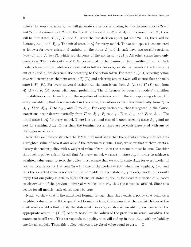
Steimle, Kaufman, and Denton: Multi-model Markov Decision Processes46
follows: for every variable ui, we will generate states corresponding to two decision epochs 2i− 1
and 2i. In decision epoch 2i− 1, there will be two states, A′i and Ai. In decision epoch 2i, there
will be four states, T ′i , F′i , Ti, and Fi. After the last decision epoch (at time 2n+ 1), there will be
2 states, An+1 and A′n+1. The initial state is A′1 for every model. The action space is constructed
as follows: for every existential variable ui, the states A′i and Ai each have two possible actions,
true (T) and false (F), which are elements of the action set {T,F}. All other states have only
one action. The models of the MMDP correspond to the clauses in the quantified formula. Each
model’s transition probabilities are defined as follows: for every existential variable, the transitions
out of A′i and Ai are deterministic according to the action taken. For state A′i (Ai), selecting action
true will ensure that the next state is T ′i (Ti) and selecting action false will ensure that the next
state is F ′i (Fi). For every universal variable ui, the transitions from A′i (Ai) to T ′i (Ti) and from
A′i (Ai) to F ′i (Fi) occur with equal probability. The differences between the models’ transition
probabilities occur depending on the negation of variables within the corresponding clause. For
every variable ui that is not negated in the clause, transitions occur deterministically from T ′i to
Ai+1, F ′i to A′i+1, Ti to Ai+1, and Fi to A′i+1. For every variable ui that is negated in the clause,
transitions occur deterministically from T ′i to A′i+1, F ′i to Ai+1, Ti to A′i+1, and Fi to Ai+1. The
initial state is A′1 for every model. There is a terminal cost of 1 upon reaching state A′n+1 and no
cost for reaching An+1. Other than the terminal costs, there are no costs associated with any of
the states or actions.
Now that we have constructed the MMDP, we must show that there exists a policy that achieves
a weighted value of zero if and only if the statement is true. First, we show that if there exists a
history-dependent policy with a weighted value of zero, then the statement must be true. Consider
that such a policy exists. Recall that for every model, we start in state A′1. In order to achieve a
weighted value equal to zero, the policy must ensure that we end in state An+1 for every model. If
not, we incur a cost of 1 at time 2n+ 1 in one of the models m∈M which has weight λm > 0, and
thus the weighted value is not zero. If we were able to reach state An+1 in every model, this would
imply that our policy is able to select actions for states A′i and Ai for existential variables ui based
on observation of the previous universal variables in a way that the clause is satisfied. Since this
occurs for all models, each clause must be true.
Next, we show that if the quantified formula is true, then there exists a policy that achieves a
weighted value of zero. If the quantified formula is true, this means that there exist choices of the
existential variables that satisfy the statement. For every existential variable ui, one can select the
appropriate action in {T,F} so that based on the values of the previous universal variables, the
statement is still true. This corresponds to a policy that will end up in state An+1 with probability
one for all models. Thus, this policy achieves a weighted value equal to zero. �
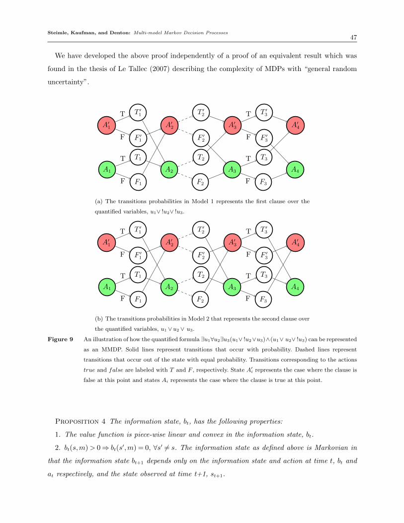
Steimle, Kaufman, and Denton: Multi-model Markov Decision Processes47
We have developed the above proof independently of a proof of an equivalent result which was
found in the thesis of Le Tallec (2007) describing the complexity of MDPs with “general random
uncertainty”.
A′1
T ′1
F ′1
T1
A1
F1
A′2
A2
T ′2
F ′2
T2
F2
A′3
A3
T ′3
F ′3
T3
F3
A′4
A4
T
F
T
F
T
F
T
F
(a) The transitions probabilities in Model 1 represents the first clause over the
quantified variables, u1∨ !u2∨ !u3.
A′1
T ′1
F ′1
T1
A1
F1
A′2
A2
T ′2
F ′2
T2
F2
A′3
A3
T ′3
F ′3
T3
F3
A′4
A4
T
F
T
F
T
F
T
F
(b) The transitions probabilities in Model 2 that represents the second clause over
the quantified variables, u1 ∨u2 ∨ u3.
Figure 9 An illustration of how the quantified formula ∃u1∀u2∃u3(u1∨ !u2∨u3)∧(u1∨ u2∨ !u3) can be represented
as an MMDP. Solid lines represent transitions that occur with probability. Dashed lines represent
transitions that occur out of the state with equal probability. Transitions corresponding to the actions
true and false are labeled with T and F , respectively. State A′i represents the case where the clause is
false at this point and states Ai represents the case where the clause is true at this point.
Proposition 4 The information state, bt, has the following properties:
1. The value function is piece-wise linear and convex in the information state, bt.
2. bt(s,m)> 0⇒ bt(s′,m) = 0, ∀s′ 6= s. The information state as defined above is Markovian in
that the information state bt+1 depends only on the information state and action at time t, bt and
at respectively, and the state observed at time t+1, st+1.

Steimle, Kaufman, and Denton: Multi-model Markov Decision Processes48
Proof of Proposition 4.1. We will prove this by induction. At time T + 1, the value function is
represented as:
vT+1(bT+1) = b′T+1rT+1,∀bT+1 ∈B
which is linear (and therefore piecewise linear and convex) in bT+1. Now, we perform the induc-
tion step. The inductive hypothesis is that the value function at t + 1 is piecewise linear and
convex in bt+1 and therefore can be represented by set of hyperplanes B such that vt+1(bt+1) =
maxβt+1∈Bt+1β′t+1bt+1.
vt(bt) = maxat∈A
b′trt(at) +∑
st+1∈S
γ(st+1|bt, at)vt+1(T (bt, at, st+1))
= max
aT∈A
b′trt(at) +
∑st+1∈S
( ∑m′∈M
∑st∈S
pm′(st+1|st, at)bt(st,m′)
)· vt+1(T (bt, at, st+1))
= max
at∈A
∑st∈S
∑m∈M
rmt (st, at) · bt(st,m) +∑
st+1∈S
∑m∈M
maxβt+1∈Bt+1
βt+1(st+1,m) ·∑st∈S
pm(st+1|st, at)bt(st,m)
= max
at∈A
∑st∈S
∑m∈M
rmt (st, at) +∑
st+1∈S
maxβt+1∈Bt+1
βt+1(st+1,m) · pm(st+1|st, at)
bt(st,m)
(9)
which is piece-wise linear and convex in bt. Therefore, we can represent (9) as the maximum over
a set of hyperplanes:
vt(bt) = maxβt∈Bt
{β′tbt} ,
where
Bt := {βt : βt = rt(a) +P ′t (a)βt+1, a∈A, βt+1 ∈Bt+1}.
�
Proof of Proposition 4.2 This follows directly from the definition of the information state 3 and
the definition of the conditional probabilities in (A). To elaborate, we prove this by induction: In
the initial decision epoch, s1 is observed and so for every m∈M, only the state corresponding to
(s1,m) can have a positive value. Now, suppose that at time t, only |M| values of bt are positive
and they correspond to the state-model pairs (s,m) with s= st. Then, the DM selects an action at
and a new state, st+1, is observed. At this point, only states (s,m) with s= st+1 can have positive
values. �
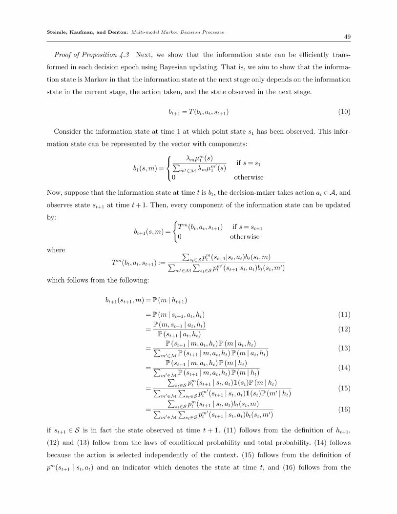
Steimle, Kaufman, and Denton: Multi-model Markov Decision Processes49
Proof of Proposition 4.3 Next, we show that the information state can be efficiently trans-
formed in each decision epoch using Bayesian updating. That is, we aim to show that the informa-
tion state is Markov in that the information state at the next stage only depends on the information
state in the current stage, the action taken, and the state observed in the next stage.
bt+1 = T (bt, at, st+1) (10)
Consider the information state at time 1 at which point state s1 has been observed. This infor-
mation state can be represented by the vector with components:
b1(s,m) =
λmµ
m1 (s)∑
m′∈M λmµm′
1 (s)if s= s1
0 otherwise
Now, suppose that the information state at time t is bt, the decision-maker takes action at ∈A, and
observes state st+1 at time t+ 1. Then, every component of the information state can be updated
by:
bt+1(s,m) =
{Tm(bt, at, st+1) if s= st+1
0 otherwise
where
Tm(bt, at, st+1) :=
∑st∈S p
mt (st+1|st, at)bt(st,m)∑
m′∈M∑
st∈S pm′t (st+1|st, at)bt(st,m′)
which follows from the following:
bt+1(st+1,m) = P (m | ht+1)
= P (m | st+1, at, ht) (11)
=P (m,st+1 | at, ht)P (st+1 | at, ht)
(12)
=P (st+1 |m,at, ht)P (m | at, ht)∑
m′∈M P (st+1 |m,at, ht)P (m | at, ht)(13)
=P (st+1 |m,at, ht)P (m | ht)∑
m′∈M P (st+1 |m,at, ht)P (m | ht)(14)
=
∑st∈S p
mt (st+1 | st, at)1(st)P (m | ht)∑
m′∈M∑
st∈S pm′t (st+1 | st, at)1(st)P (m′ | ht)
(15)
=
∑st∈S p
mt (st+1 | st, at)bt(st,m)∑
m′∈M∑
st∈S pm′t (st+1 | st, at)bt(st,m′)
(16)
if st+1 ∈ S is in fact the state observed at time t + 1. (11) follows from the definition of ht+1,
(12) and (13) follow from the laws of conditional probability and total probability. (14) follows
because the action is selected independently of the context. (15) follows from the definition of
pm(st+1 | st, at) and an indicator which denotes the state at time t, and (16) follows from the
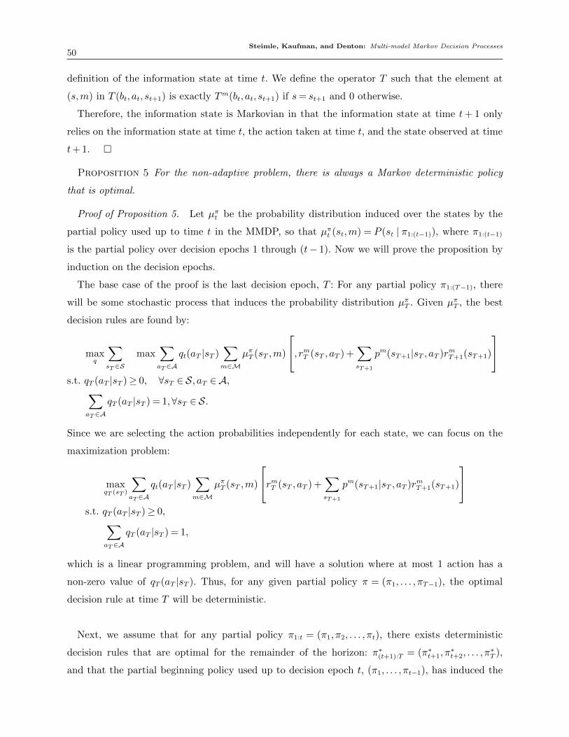
Steimle, Kaufman, and Denton: Multi-model Markov Decision Processes50
definition of the information state at time t. We define the operator T such that the element at
(s,m) in T (bt, at, st+1) is exactly Tm(bt, at, st+1) if s= st+1 and 0 otherwise.
Therefore, the information state is Markovian in that the information state at time t+ 1 only
relies on the information state at time t, the action taken at time t, and the state observed at time
t+ 1. �
Proposition 5 For the non-adaptive problem, there is always a Markov deterministic policy
that is optimal.
Proof of Proposition 5. Let µπt be the probability distribution induced over the states by the
partial policy used up to time t in the MMDP, so that µπt (st,m) = P (st | π1:(t−1)), where π1:(t−1)
is the partial policy over decision epochs 1 through (t− 1). Now we will prove the proposition by
induction on the decision epochs.
The base case of the proof is the last decision epoch, T : For any partial policy π1:(T−1), there
will be some stochastic process that induces the probability distribution µπT . Given µπT , the best
decision rules are found by:
maxq
∑sT∈S
max∑aT∈A
qt(aT |sT )∑m∈M
µπT (sT ,m)
, rmT (sT , aT ) +∑sT+1
pm(sT+1|sT , aT )rmT+1(sT+1)
s.t. qT (aT |sT )≥ 0, ∀sT ∈ S, aT ∈A,∑
aT∈A
qT (aT |sT ) = 1,∀sT ∈ S.
Since we are selecting the action probabilities independently for each state, we can focus on the
maximization problem:
maxqT (sT )
∑aT∈A
qt(aT |sT )∑m∈M
µπT (sT ,m)
rmT (sT , aT ) +∑sT+1
pm(sT+1|sT , aT )rmT+1(sT+1)
s.t. qT (aT |sT )≥ 0,∑
aT∈A
qT (aT |sT ) = 1,
which is a linear programming problem, and will have a solution where at most 1 action has a
non-zero value of qT (aT |sT ). Thus, for any given partial policy π = (π1, . . . , πT−1), the optimal
decision rule at time T will be deterministic.
Next, we assume that for any partial policy π1:t = (π1, π2, . . . , πt), there exists deterministic
decision rules that are optimal for the remainder of the horizon: π∗(t+1):T = (π∗t+1, π∗t+2, . . . , π
∗T ),
and that the partial beginning policy used up to decision epoch t, (π1, . . . , πt−1), has induced the

Steimle, Kaufman, and Denton: Multi-model Markov Decision Processes51
probability distribution µπt . We will show that it follows that there exists a deterministic decision
rule that is optimal for decision epoch t:
∑st∈S
maxq
∑at∈A
qt(at|st)∑m∈M
µπt (st,m)
rmt (st, at) +∑st+1
pm(st+1|st, at)vmt+1(st+1)
s.t. qt(at|st)≥ 0,∑
at∈A
qt(at|st) = 1.
Once again, we can focus on the maximization problem within the sum:
maxqt(at|st)=1
∑at∈A
qt(at|st)∑m∈M
µπt (st,m)
rmt (st, at) +∑st+1
pm(st+1|st, at)vmt+1(st+1)
s.t. qt(at|st)≥ 0,∑
at∈A
qt(at|st) = 1.
This is a linear program so there will exist an extreme point solution that is optimal. This extreme
point solution corresponds to a deterministic decision rule for decision epoch t. �
Proposition 6 Solving the non-adaptive problem for an MMDP is NP-hard.
Proof of Proposition 6. We show that any 3-CNF-SAT problem can be transformed into the
problem of determining if there exists a Markov deterministic policy for an MMDP such that
the weighted value is greater than zero. Let’s suppose we have a 3-CNF-SAT instance: a set of
variables U = {u1, u2, . . . , un} and a formula E = C1 ∧ C2 . . . ∧ Cm. We will construct an MMDP
with one decision epoch from this instance of 3-CNF-SAT. In the only decision epoch, the state
space consists of one state per variable, ui, i= 1, . . . , n. At the terminal stage, there are two states
labeled “T” and “F”. There are no immediate rewards for this problem. For every state ui, there
are two actions true or false. The terminal rewards correspond to a cost of 0 for reaching the
terminal state “T” and a cost of 1 upon reaching the terminal state “F”.
The transition probabilities for model j correspond to the structure of clause Cj and are defined
as follows: for any variable ui, i < n that does not appear in Clause j, both actions lead to the
state ui+1 with probability 1. If variable un does not appear in Clause j, both actions lead to the
state “F” with probability 1. For any variable ui that appears non-negated in clause Cj, the action
true leads from state ui to state “T” with probability 1 and the action false leads from state ui
to state ui+1 with probability 1. For the variables that appear negated in the clause, the action
true leads from state ui to state ui+1 with probability 1 and the action false leads from state ui to
state “T” with probability 1. The initial distribution of all models is variable u1 with probability
1.

Steimle, Kaufman, and Denton: Multi-model Markov Decision Processes52
We will show that there is a truth assignment for the variables in U that satisfies E if and only
if there is a Markov deterministic policy for the MMDP that achieves a weighted value equal to 0.
First, we show that if there is a truth assignment for the variables in U that satisfies E, then
there exists a Markov deterministic policy for the MMDP that achieves a weighted value equal
to 0. To construct such a policy, take the action true in every state ui such that ui is true is
the satisfying truth assignment and take the action false otherwise. Because this true assignment
satisfies each clause, the corresponding policy will reach state “T” with probability 1 in each model.
By construction, this policy will have a weighted value of zero.
Next, we show that if there is a policy Π = ΠMD that achieves a weighted value of 0, that there
exists a truth assignment that will satisfy E. Suppose that policy π ∈ΠMD achieves a cost of zero.
This implies that for every clause, the policy π leads to the state “T” with probability 1. We can
construct a truth assignment from this policy by assigning ui to be true if π(ui) is true, and ui to
be false if π(ui) is false.
Therefore, we have created a one-to-one mapping of truth assignments to MD policies such that
any policy that satisfies E will also have weighted value 0. Hence, if we were able to find a policy
that achieves a weighted value of 0 in polynomial time, we would also be able to solve 3-CNF-SAT
in polynomial time. Thus, the MMDP weighted value problem with Π = ΠMD is NP-hard. �
u1
u2
u3
u4
T
F
falsetrue
true
false
true
false
(a) The transitions probabilities in
model 1 that represent the first clause:
C1 =!u1∨ !u2 ∨u3.
u1
u2
u3
u4
T
F
truefalse
false
true
false
true
(b) The transitions probabilities in
model 2 that represent the second
clause: C2 = u1 ∨u2∨ !u4.
Figure 10 An illustration of how a 3-CNF-SAT instance, E = (u1∨ !u2 ∨u3)∧ (u1 ∨ u2∨ !u4), can be represented
as an MMDP. Solid lines represent the transitions associated with the action true and dashed lines rep-
resent the transitions associated with the action false. All transitions shown happen with probability
1.

Steimle, Kaufman, and Denton: Multi-model Markov Decision Processes53
Proposition 7. Non-adaptive MMDPs can be formulated as the following MIP:
maxv,x
∑m∈M
λm∑s∈S
µm1 (s)vm1 (s)
s.t. vmT+1(s) ≤ rmT+1(s), ∀s∈ S,m∈M,
vmt (s) ≤ rmt (s, a) +∑s′∈S
pmt (s′|s, a)vmt+1(s′) +M(1−xs,a,t), ∀m∈M, s∈ S, a∈A,
t∈ T ,∑a∈A
xs,a,t = 1, ∀s∈ S, t∈ T ,
xs,a,t ∈ {0,1}, ∀s∈ S, a∈A, t∈ T .
(17)
Proof of Proposition 7 The decision variable vt(s) represents the optimal value-to-go for state
s ∈ S at time t ∈ T . The dual variables correspond to the probability of selecting an action given
a state. Corner point solutions correspond to deterministic policies, and the optimal policy is
deterministic by construction.
For an MMDP, we cannot use the standard LP formulation used to solve MDPs because of the
requirement that the policy must be the same in each of the different models. The mixed-integer
program shown in (17) gives a formulation that ensures that the policy π ∈ ΠMD is the same in
each model. Each decision variable, vmt (s) represents the value-to-go from state s∈ S at time t∈ T
for model m ∈M corresponding to the policy π ∈ΠMD that maximizes the weighted value of the
MMDP. To enforce that the same policy in each model, m ∈M, we introduce binary decision
variables, xs,a,t for every state, s ∈ S, action, a ∈ A, and decision epoch t ∈ {1,2, . . . , T}. If xs,a,t
takes on a value of 1, this means that the best policy dictates taking action a in state s at time t
for every model, and xs,a,t = 0 otherwise. If the choice of M is sufficiently large (e.g., M > (|T |+
1) ·maxm∈M,s∈S,a∈A,t∈T rt(s, a)), then the inequalities will become tight when the corresponding
binary decision variable xs,a,t = 1, because all of the other actions’ constraints will have a large
value, M , added to their value in the second inequality. The equality constraint ensures that every
state-time pair only has one action prescribed. �
Proposition 8. For any policy π ∈Π, the weighted value is bounded above by the weighted sum
of the optimal values in each model. That is,∑m∈M
λmvm(π)≤
∑m∈M
λm maxπ∈ΠMD
vm(π), ∀π ∈Π
Proof of Proposition 8 The result follows from this series of inequalities:∑m∈M
λmvm(π)≤ max
π∈ΠMD
∑m∈M
λmvm(π) (18)
≤∑m∈M
λm maxπ∈ΠMD
vm(π),

Steimle, Kaufman, and Denton: Multi-model Markov Decision Processes54
where (18) states than any MD policy will have a weighted value at most the optimal MD policy’s
weighted value. This optimal weighted value, in turn, is at most the value that can be achieved by
solving each model separately and then weighting these values. �
Proposition 9 WSU is not guaranteed to produce an optimal solution to the non-adaptive
weighted value problem.
Figure 11 An illustration of an MMDP for which the WSUapproximation algorithm does not generate an optimal
solution to the non-adaptive weighted value problem. Possible transitions for actions 1 and 2 are
illustrated with the dashed and solid line respectively. The probability of each possible transition in
both of the models is listed by the corresponding line. The DM receives a reward of 1 if state D is
reached. Otherwise, no rewards are received.
Proof of Proposition 9. Consider the counter-example illustrated in Figure 11 for λ1 = 0.8, λ2 =
0.2. The MMDP has 5 states, 2 actions, 2 models, and 2 decision epochs. First, we can explicitly
enumerate all possible deterministic policies for the non-adaptive weighted value problem.
By explicitly enumerating all of the possible deterministic policies, we see that selecting action 1
for state A and action 1 for state B leads to the maximum expected weighted value of 0.9λ2 = 0.72.
Now, consider the resulting policy generated from WSU. There is only one option for state C, so
WSU will select π(C) = 1 and update the value for each model as v1(C) = 0 and v2(C) = 0. For
state B, WSU will select:
π(B)← arg maxa∈{1,2}
{λ1p1(D|B,a) +λ2p
2(D|B,a)}
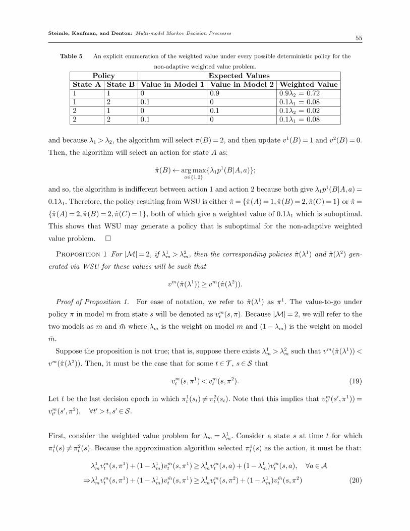
Steimle, Kaufman, and Denton: Multi-model Markov Decision Processes55
Table 5 An explicit enumeration of the weighted value under every possible deterministic policy for the
non-adaptive weighted value problem.
Policy Expected ValuesState A State B Value in Model 1 Value in Model 2 Weighted Value1 1 0 0.9 0.9λ2 = 0.721 2 0.1 0 0.1λ1 = 0.082 1 0 0.1 0.1λ2 = 0.022 2 0.1 0 0.1λ1 = 0.08
and because λ1 >λ2, the algorithm will select π(B) = 2, and then update v1(B) = 1 and v2(B) = 0.
Then, the algorithm will select an action for state A as:
π(B)← arg maxa∈{1,2}
{λ1p1(B|A,a)};
and so, the algorithm is indifferent between action 1 and action 2 because both give λ1p1(B|A,a) =
0.1λ1. Therefore, the policy resulting from WSU is either π= {π(A) = 1, π(B) = 2, π(C) = 1} or π=
{π(A) = 2, π(B) = 2, π(C) = 1}, both of which give a weighted value of 0.1λ1 which is suboptimal.
This shows that WSU may generate a policy that is suboptimal for the non-adaptive weighted
value problem. �
Proposition 1 For |M|= 2, if λ1m >λ
2m, then the corresponding policies π(λ1) and π(λ2) gen-
erated via WSU for these values will be such that
vm(π(λ1))≥ vm(π(λ2)).
Proof of Proposition 1. For ease of notation, we refer to π(λ1) as π1. The value-to-go under
policy π in model m from state s will be denoted as vmt (s,π). Because |M|= 2, we will refer to the
two models as m and m where λm is the weight on model m and (1−λm) is the weight on model
m.
Suppose the proposition is not true; that is, suppose there exists λ1m >λ
2m such that vm(π(λ1))<
vm(π(λ2)). Then, it must be the case that for some t∈ T , s∈ S that
vmt (s,π1)< vmt (s,π2). (19)
Let t be the last decision epoch in which π1t (st) 6= π2
t (st). Note that this implies that vmt′ (s′, π1)) =
vmt′ (s′, π2), ∀t′ > t, s′ ∈ S.
First, consider the weighted value problem for λm = λ1m. Consider a state s at time t for which
π1t (s) 6= π2
t (s). Because the approximation algorithm selected π1t (s) as the action, it must be that:
λ1mv
mt (s,π1) + (1−λ1
m)vmt (s,π1)≥ λ1mv
mt (s, a) + (1−λ1
m)vmt (s, a), ∀a∈A
⇒λ1mv
mt (s,π1) + (1−λ1
m)vmt (s,π1)≥ λ1mv
mt (s,π2) + (1−λ1
m)vmt (s,π2) (20)
Steimle, Kaufman, and Denton: Multi-model Markov Decision Processes56
Next, consider the weighted value problem for λm = λ2m. In this case, for the same state s as above,
it must be that the approximation algorithm selected action π2t (s) because:
λ2mv
mt (s,π2) + (1−λ2
m)vmt (s,π2)≥ λ2mv
mt (s, a) + (1−λ2
m)vmt (s, a), ∀a∈A
⇒λ2mv
mt (s,π2) + (1−λ2
m)vmt (s,π2)≥ λ2mv
mt (s,π1) + (1−λ2
m)vmt (s,π1). (21)
Rearranging (20), we have
λ1(vmt (s,π1)− vmt (s,π2)) + (1−λ1m)(vmt (s,π1)− vmt (s,π2))≥ 0, (22)
and rearranging (21), we have
λ2m(vmt (s,π2)− vmt (s,π1)) + (1−λ2
m)(vmt (s,π2)− vmt (s,π1))≥ 0 (23)
⇒−λ2m
(vmt (s,π1)− vmt (s,π2)
)− (1−λ2
m)(vmt (s,π1)− vmt (s,π2)
)≥ 0. (24)
Adding (22) and (24), we have:
(λ1m−λ2
m)(vmt (s,π1)− vmt (s,π2)
)+((1−λ1
m)− (1−λ2m)) (vmt (s,π1)− vmt (s,π2)
)≥ 0
⇒(λ1m−λ2
m)(vmt (s,π1)− vmt (s,π2) + vmt (s,π2)− vmt (s,π1)
)≥ 0. (25)
Because λ1m >λ
2m, it must be that
vmt (s,π1)− vmt (s,π2) + vmt (s,π2)− vmt (s,π1)≥ 0
⇒vmt (s,π2)− vmt (s,π1)≥ vmt (s,π2)− vmt (s,π1)
⇒vmt (s,π2)> vmt (s,π1), (26)
where (26) follows because of (19). However, because vmt (s,π1) < vmt (s,π2) and vmt (s,π1) <
vmt (s,π2), this implies that
λ1mv
mt (s,π1) + (1−λ1
m)vmt (s,π1)<λ1vmt (s,π2) + (1−λ1m)vmt (s,π2),
which contradicts that the approximation algorithm would have selected action π1t (s) for the
weighted value problem with λm = λ1m. Therefore, it must be the case that if λ1
m >λ2m, then
vm(π(λ1))≥ vm(π(λ2)).
�
Proposition 10 For |M|= 2, any policy generated via WSU will be such that
W (π(λ))≥ λv1(π2) + (1−λ)v2(π1),
where πm is the optimal policy for model m.

Steimle, Kaufman, and Denton: Multi-model Markov Decision Processes57
Proof of Proposition 10. Let λ be the weight on model 1, π1 be an optimal policy for model
1, and π2 be an optimal policy for model 2. Due to the result of Proposition 1, it follows that
v1(π(λ))≥ v1(π2) = v1(π(0)), ∀λ∈ [0,1],
v2(π(λ))≥ v2(π1) = v2(π(1)), ∀λ∈ [0,1],
and therefore,
W (π(λ)) = λv1(π(λ)) + (1−λ)v2(π(λ))≥ λv1(π2) + (1−λ)v2(π1).
�
Appendix B: Solution methods for the adaptive problem
In this appendix, we describe an exact solution method that can be used to solve the adaptive
problem for an MMDP. We begin by describing Procedure 2 which is an exact solution method for
solving the adaptive weighted value problem. The correctness of this solution method follows from
Proposition 2 which states that every MMDP is a special case of a POMDP and that the maximum
weighted value is equivalent to the expected discounted rewards of the corresponding POMDP.
Therefore, we transform the MMDP into a POMDP and use a solution method analogous to a
well-known solution method for POMDPs (Smallwood and Sondik 1973). This method exploits
the property that the value function is piece-wise linear convex and therefore can be represented
as the maximum over a set of supporting hyperplanes (Proposition 4).
In the worst-case, the number of hyperplanes needed to represent the value function could
potentially be as large as 1 + |A|+∑T−1
t=1 |A||S|+T−t for T ≥ 2, but in many cases the number of
hyperplanes that are actually needed to represent the optimal value function is much smaller.
Pruning describes the methods by which hyperplanes that are not needed to represent the optimal
value function are discarded. The pruning method described in Procedure 3 is based on the LP
method described in Smallwood and Sondik (1973), but exploits the result of Proposition 2 for
computational gain. This result states that only certain parts of the information space are reachable
due to the special structure of the MMDP and this allows for the LP problems for pruning to be
decomposed into a set of smaller LPs.
For this procedure, we will use the information state as defined in Definition 3 and define the
following notation:
rmT+1 :=
rT+1(1)...
rT+1(|S|)
, rmt (at) :=
rt(1, at)...
rt(|S|, at)
,∀m∈M,∀at ∈A,

Steimle, Kaufman, and Denton: Multi-model Markov Decision Processes58
rT+1 :=
r1T+1...
r|M|T+1
, rt(at) :=
r1t (at)
...
r|M|t (at)
,∀at ∈A,For every action, we define the block diagonal matrix:
Pt(at) :=
P 1t (at) 0 . . . 00 P 2
t (at) . . . 0...
.... . .
...0 0 . . . PM
t (at)
,where each matrix Pm
t (at), ∀m ∈ M is the transition probability matrix in decision epoch t ∈
T associated with action at ∈ A for model m ∈M. The matrix Q represents the analog of the
conditional probability matrix for observations:
Q := [I|S|, . . . , I|S|︸ ︷︷ ︸|M| times
]′,
where I|S| denotes an |S| × |S| identity matrix. We use Q(st) to denote the column vector corre-
sponding to st ∈ S such that the elements indexed (s,m) in this vector have values
q(st|(s,m)) =
{1 if s= st0 otherwise
for all m∈M.
The space of all information states at time t is
Bt =
{bt : bt(s,m)≥ 0, ∀(s,m)∈ S ×M,
∑m∈M
bt(s,m) = 1,∀s∈ S
}.
Procedure 2 is a backwards induction algorithm which generates a set of hyperplanes at each
decision epoch. Procedure 3 eliminates hyperplanes that are not necessary to represent the optimal
value function. The DM selects the optimal sequence of actions for the observed history in an
analogous way to a POMDP: update the information state based on the observation and select the
action corresponding to the maximizing hyperplane at this particular information state.

Steimle, Kaufman, and Denton: Multi-model Markov Decision Processes59
Procedure 2 Algorithm for solving the adaptive weighted value problem (2)
Input: MMDP
Initialize BT+1 = {rT+1}
The value-to-go at time T + 1. vT+1(bT+1) = β′T+1bT+1, ∀bT+1 ∈BT+1
t← T
while t≥ 0 do
for Every action at do
Bt(at)←{βt(at) : βt(at) = rt(at) +
∑st+1∈S
Pt(at)diag(Q(st+1))βst+1t+1 ,
∀β1t+1× · · ·×β
|S|t+1 ∈Bt+1× · · ·×Bt+1
}end for
Bt←∪at∈ABt(at)
State-wise Prune(Bt)
The value-to-go at time t is vt(bt) = maxβt∈Bt β′tbt, ∀bt ∈Bt
t← t− 1
end while
Output: Collection B0, . . . ,BT
Procedure 3 State-wise PruneInput: A set of vectors in R|S×M|, B.
for Every vector β ∈B do
for Every state s∈ S do
Let B(s) = {βs : βs(m) = β(s,m), β ∈B}
Solve the LP (27)
z∗s := minµs∈M (M),x∈R
x−β′sµs (27)
s.t. x≥ β′sµs ∀βs ∈B(s),∑m∈M
µs(m) = 1
If∏s∈S z
∗s > 0, remove β from B.
end for
end for
Output: B


![QIP = PSPACE · extend this result to all of QIP, establishing the relationship QIP =PSPACE. Similar to [JUW09], we use the matrix multiplicative weights update method, together with](https://static.fdocuments.us/doc/165x107/5f88586338174314853ac9c8/qip-pspace-extend-this-result-to-all-of-qip-establishing-the-relationship-qip.jpg)