Multi-layered Interbank Model for AssessingSystemic Risk

Mattia Montagna , Christoffer Kok∗

September 12, 2013

AbstractIn this paper, we develop an agent-based multi-layered interbank net-

work model based on a sample of large EU banks. The model allows fortaking a more holistic approach to interbank contagion than is standard inthe literature. A key finding of the paper is that there are non-negligiblenon-linearities in the propagation of shocks to individual banks when tak-ing into account that banks are related to each other in various marketsegments. In a nutshell, the contagion effects when considering the shockpropagation simultaneously across multiple layers of interbank networkscan be substantially larger than the sum of the contagion-induced losseswhen considering the network layers individually. In addition, a bank “sys-temic importance” measure based on the multi-layered network model isdeveloped and is shown to outperform standard network centrality indi-cators.

JEL Classification: C45, C63, D85, G21

Key words: Financial contagion, interbank market, network theory

1 IntroductionDuring the financial crisis that emerged in 2007 a large part of the global finan-cial system came under stress with severe repercussions on the real economy.The sequence of events which unfolded from the summer of 2007 forced publicsectors to intervene in order to restore financial stability which in turn put pres-sure on public finances in many EU Countries. The costs associated with thoseinterventions highlighted the importance of safeguarding in a stable financialsystem.

A stable financial system should not propagate or magnify shocks to otherpart of the system itself, nor to the real economy. Systemic risk, in the view ofthis paper, exactly refers to the possibility that the financial system evolves in aconfiguration which makes it particularly prone to global breakdowns in case ofan initial local shock. The reasons why the system can arrive to such unstable∗The authors would like to thank Thomas Lux for valuable comments and Grzegorz Halaj

for making available the data and for fruitful discussions.

1

configurations are probably rooted in the duality among local and global prop-erties of the financial system. In other words, each financial institution takesits decisions with the aim of maximizing its own profits and interests, but itdoes not internalize the impacts of its actions on the stability of the system aswhole. Moreover, as we will show in this paper, also if banks were willing tominimize systemic risk when they take decisions, they would need to have suffi-cient information regarding the financial situations of the other banks, includingthe exposures each bank have on each other. As an example, one can considerthe direct exposures in an interbank market. If one bank wants to evaluate theriskiness associated with a loan to another bank, it should be able to know theexposures of its counterparty, which probability of default depends on its owncounterparties, and so on. No bank is able to peer so deeply into the interbankcredit network to evaluate the probability of defaults due to contagion effects.

A crucial role in ensuring financial stability is therefore played by informa-tion. If the ultimate goal is to reduce systemic risk, it is necessary to have aglobal view of the financial system in order to identify and monitor possiblesources and channels of contagion. A robust framework for monitoring and as-sessing financial stability, and for managing it with interventions able to preventthe system from entering into critical configurations, must be able to evaluatethe continuously evolving structure of the financial system. Another impor-tant lesson emerging from the recent financial crisis that we try to account forin this paper is that the possible sources of systemic instability are multiple.For instance, direct bilateral exposures can create domino effects and propagateidiosyncratic (or local) shocks to the wides (global) financial system. In addi-tion, forced firesales of financial assets can lead to strong asset price declinesand can transmit losses through banks with common exposures and overlappingportfolios. Furthermore, news about a firm’s assets can signal that others withsimilar assets may also be distressed and thus create widespread market uncer-tainty. Moreover, the sudden interruption of a service provided by a bank tothe financial system can constitute a threat in case other banks are not able toimmediately substitute it.

Against this background, the aim of this paper is to study systemic risk inhighly interconnected financial systems. A natural way to represent and studyan interbank market is network theory, nowadays commonly used in finance. Inorder to encapsulate the different kinds of possible connections among banks,we use a multi-layered network model. A multi-layered network is a systemwhere the same set of nodes belong to different layers, and each layer is char-acterized by its own kind of edge (representing a particular kind of financialconnection), by its own topology (so each node may have different neighbors indifferent layers), and its own rules for the propagation of eventual shocks. Thisholistic view of the financial system should enable us to study systemic risk in amore encompassing perspective, than typical single-layered network structuresfocusing on individual segments.

On top of the multi-layered system we put an agent-based model whereagents can interact with each other through the network structure. The stan-dard approach in the literature to study systemic risk using network theory isto assume passive banks as nodes in the network1. Those kinds of models are

1A pioneering work in this direction was initially proposed by Nier et al. (2009), while asummary of the results coming from this branch of literature can be found in Upper (2011).

2

good at estimating the resilience of particular network structures against shocks,but they lack real dynamic effects, since shocks propagate through the systemwithout incorporating the (likely) reaction of banks to those shocks. The intro-duction of agents enable us to investigate specific network structures in combina-tion with a plausible bank behavior. In particular, in our model banks will onlyadjust their balance sheets when endogenous or exogenous shocks bring theirliquidity or their risk-weighted capital ratio below the minimum requirements.In fact, if we assume that prior to the shock the system was in equilibrium, bankswould just try to keep the same structure of their balance sheets also during thepropagation of the shock. The failure of a financial institution usually impliesseveral repercussions on the system. As already highlighted, the liquidation ofa failed bank can push prices down, its counterparts can book losses from directbilateral exposures, the financial services provided by the bank cannot alwaysbe replaced, at least not immediately, and the combination of such reactionscan significantly amplify shocks and lead to dangerous spirals which could po-tentially collapse substantial parts of the financial system ( ... Brunnermeier(2009)). The complete dynamics of such events is difficult to capture with ana-lytical models and from this perspective an agent-based model is more suitable,since it enables studying also systems out of equilibrium.

The agent-based model combined with the multi-layered network is subse-quently used to design measures for the systemic importance of each bank inthe system. Those measures rely on information regarding direct and indirectinterbank connections, which can be inferred from network theory, and banksbalance sheet information. The basic notion is that standard network centralitymeasures alone cannot explain the systemic importance of individual financialinstitutions, since the high level of heterogeneity in banking systems can bringcentral capitalized nodes to stabilize the system, whereas only network measureswould just judge nodes depending on their centrality. Instead, it is necessary tocombine information regarding the balance sheet structure of institutions withmeasures of centrality in order to understand the impact of each bank failureon the system.

This paper is organized as follows: section 2 reviews the main literaturelinked to our work, highlighting both the contributions in the multi-layerednetwork theory and the agent-based interbank models; section 3 introduces themulti-layered interbank market and explains how the structure is calibrated on areal dataset; section 4 explains the model we use for investigating systemic risk;section 5 presents details about the implementation of the model and the resultsfrom our simulation engine; section 6 introduces our measures for the systemicimportance banks, and shows how the measures can be used to monitor systemicrisk in the system; section 7 concludes and provides some policy implications.

2 Literature ReviewIn the past years, especially after the last financial crisis, more and more re-searchers have point their efforts to study the financial system, and in particularthe banking sector, from a network perspective. The first contribution in thatdirection can be probably recognized in Allen and Gale (2000); starting fromthe model of Diamond and Dybvig (1983), they introduce an interbank liquiditymarket which enables banks to insurance each other against liquidity shocks.

3

Although in normal conditions this interbank market can improve the stabilityof the financial system, in case a large shock hits one of the banks, the bankmay fail and induce losses to its counterparties; in turn, these losses can po-tentially cause other defaults, therefore creating a domino effect. The authorshow that when the underlying network structure is complete (each bank is con-nected to all the other) the system is much more resilient due to risk sharing,while incomplete networks are much more fragile since banks find more difficultto share proper idiosyncratic shocks with their few counterparties. Nier et al(2009) show in their work how the topological features of the interbank networkcan be related to the financial stability of the system. Surprisingly, the resultshighlight that the higher the risk-sharing among banks, the higher the size ofthe domino effect (up to a certain threshold value for the banking connectivity)in case of a shock hits one of the bank in the system. Furthermore, they showthat increasing the level of capitalization will reduce the number of defaults incase of a shock hits the system, and this effect is strongly non linear. Otherworks about interbank network, e.g. Gai and Kapadia (2010), clearly show thedualism of interbank connections: on one side, they are necessary in order topool idiosyncratic risk of single institutions and improve the efficiency of thebanking sector. In Iori et al (2006) a dynamic model of the banking system,where banks can interact each other through interbank loans, is used to showthe stabilizing role of the interbank lending. On the other side, interbank con-nections turn to be channels for the propagation of local shocks through thewhole system. A summary of the results coming from this branch of literaturecan be found in Upper (2011).

In the view of regulators, it becomes therefore necessary to measure andmonitor the stability of the banking system as a whole, in parallel to the sit-uation of the single financial institutions. In this respect, different measuresof systemic risk have been developed, and a taxonomy of these measures isprovided for example in Bisias et al (2012). We focus here only on measuresbased on network analysis and systemic financial linkages. In Eisenberg andNoe (2001) they provide a recursive algorithm to find the clearing paymentvector that clears the obligations of a set of financial firms, and at the sametime it provides information about the systemic risk faced by each institution.In Battiston et al (2012) a measure based on network feedback centrality isintroduced, the so-called DebtRank; this measure is used to analyze a datasetconcerning the FED emergency loans program to global financial institutionsduring the period 2008-2010. The results show how, at the peak of the crisis,all the largest institutions served by the FED program became systemically im-portant at the same time. In Halaj and Kok (2013) they present an approachto generate interbank networks with realistic topologies, and they expand theEisenberg and Noe (2001) algorithm to include firesales effect; remarkably, thisis one of the few contributions where the network structure has not a randomtopology. Delpini et al (2013) study the Italian electronic trading system (e-MID) with tools borrowed from statistical physics to find the key players ona liquidity overnight market; interestingly, the drivers of the market, ie thatnodes which are crucial for the functioning of the interbank market, are oftennot the hubs neither the largest lenders in the system. We highlight that in allthese contributions, results are always restricted to contagion or spillover effectsrelated to one particular segment of the interbank market, which usually is theinterbank claims banks have on each other.

4

The branch of literature closer to our contribution is probably the one con-cerning dynamic interbank models. These discrete-time models usually allow toinclude some realistic microeconomic behavior for the banks on top of the net-work structure. An example can be found in Bluhm and Krahnen (2011). Theauthors study systemic risk in a banking system where financial institutions arelinked each other through interbank lending, and firesales by one institutionsaffect the capital of all the others, since the price of the (mark-to-market) assetsin the secondary market is endogenous in the model, and driven by the liquidityneeds of the banks. The authors also introduce a game-theoretical approach toidentify the contribution of each bank to systemic risk, and use this measure todevelop an optimal charge to reduce financial instability. Georg (2011) developsa dynamics banking system where banks are allowed to optimize their portfoliosof investments and they receive random fluctuation in their deposits; with thisagent-based model, the author shows how the topology of the interbank marketaffects the stability of the system. In particular, he shows that contagion effectsare larger in random network than in scale-free network, the classical structureof real world networks. He also investigates the role of the central bank in theinterbank market, and in particular how the level of collateral which is acceptedby the central bank affects financial stability; the results show that an abundantprovision of liquidity by the central bank leads to a reduction of the liquiditybanks exchange each other on the interbank market. Ladley (2011) develops amodel of a closed economy composed of households which can deposit their fundsin a banking system and require loans for their private investments, and bankswhich learn through genetic algorithm how to better allocate their resources inorder to maximize their expected returns. Since banks can lend also among eachother, bad investments taken by households can trigger domino effects amongthe banks in the system. Banks in the model are subject to regulation, and theaim of the model is to qualitatively show the link among regulation, interbanknetwork structure, and the likelihood of a contagion. The results state that forhigh levels of connectivity the system is more stable when the shock is small,while the spillover effects are amplified in case of larger initial shocks.

Despite the huge number of contributions in network theory aimed at theidentification of important nodes in a graph, still lot of work has to be donefor what regards multi-layered (ML) network. In a lot of different fields, fromtelecommunication engineering to sociology, ML system are a natural represen-tation of the reality. Examples are the Open Systems Interconnections (OSI)model, used to abstract the real internal structure of a communication systeminto different functionality layers, or the several ML social network model whichencapsulate in different layers the different natures of possible social connec-tions among people. Financial systems are another example of multi-layerednetwork, given the several kinds of connections that can exist among banksbalance sheets. Recently, Gomez et al (2012) showed that a diffusion process,modeled as a flow traveling on the network from node to node, can be extremelyamplified in case of multiple layers connect the same set of nodes. The linearequations they propose in order to analyze the model are hardly applicable tocases when the nodes have a non trivial internal structure and the contagionmechanisms change from layer to layer, but the results clearly claim the neces-sity to study ML systems from a different perspective than their single-layeredcounterparty.

5

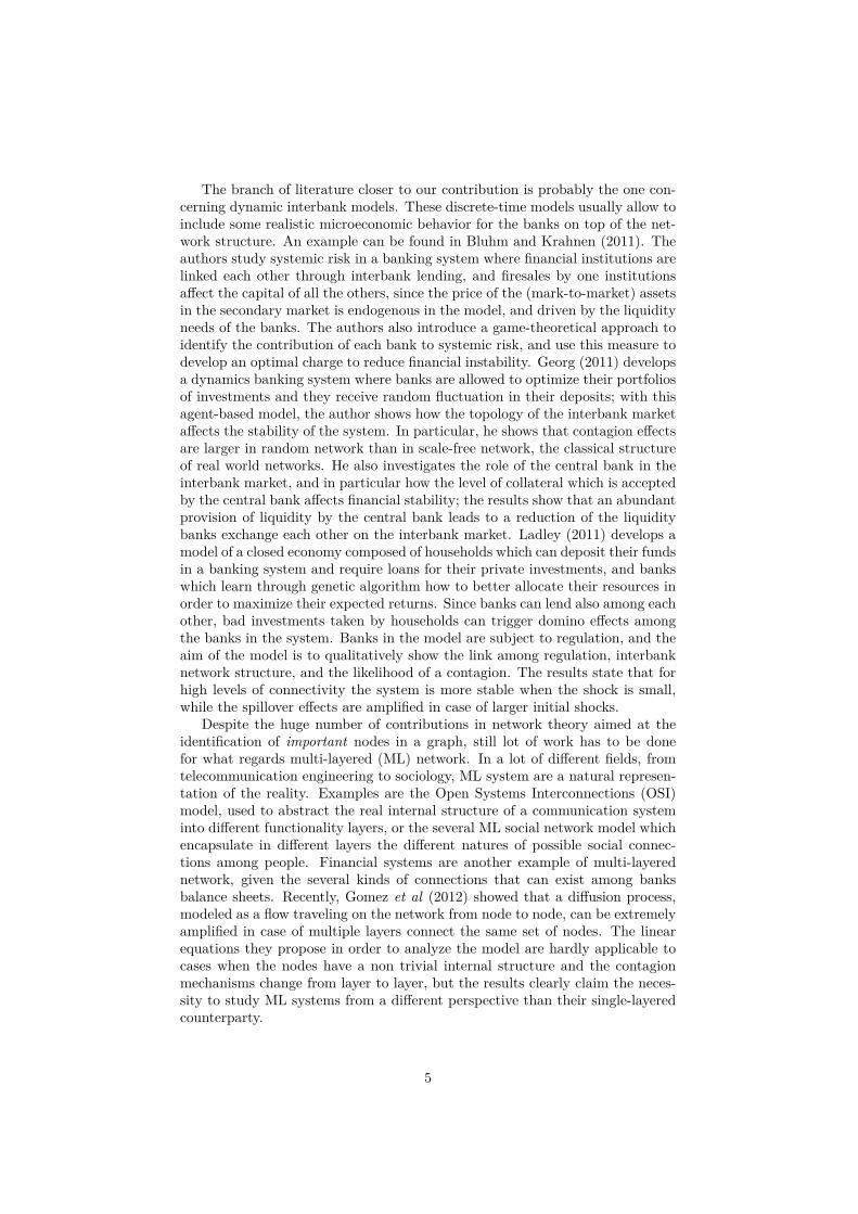
Figure 1: An exam-ple of triple-layered net-work, where the sameset of nodes belong toeach of the three lay-ers, characterized by itsown topology. The firsttwo layers contain di-rected networks, mean-while the last one is undi-rected. The differentneighbors in the differ-ent layers give the multi-layered networks com-pletely different systemdynamics during shockpropagation, since thenumber of affected nodescan drastically be in-creased due to the multidimensional structure ofthe system.

3 Multi-Layered Financial SystemsA natural way to study highly interconnected systems is network theory. Net-work theory provides a rich set of tools to assess the centrality (or systemicimportance) of the members of a network of nodes. In this paper, each nodein the network represents a bank; importantly each node will be equipped witha non-trivial internal structure, representing the banks’ balance sheets. This iscrucial, since abstracting from a realistic internal structure for the node meansto disregard the realistic and interesting effects linked to limited liabilities andcapital absorption. Moreover, a key aspect of this paper is to analyze the in-terconnectedness between banks in a multi-dimensional space. Banks in realityare connected through several kinds of relationships, directed and undirected,with different maturities. In order to encapsulate this level of complexity, weuse a multi-layered instead of a single-layered network. We formally denote amulti-layered network by a triple G = (V , W,L), where V is a set of nodes,common to all the layers, L is a set of labels indicating the different layers,W =

(W 1,W 2, . . . ,W l

)is a set of matrices, with the same cardinality of L,

representing the network topologies in the different layers.We want to concentrate in particular on three layers, which represent three

different kinds of dependencies among banks that were reveled to be funda-mental during the last financial crisis: (i) long-term, direct bilateral exposures,reflecting the lending-borrowing network; (ii) short-term direct bilateral expo-sures, reflecting the liquidity network; and (iii) common exposures to financialassets, measuring the network of overlapping portfolios2. Consequently, we will

2It should be noted that several other layers can be added to the multi-layered framework,for example the layers representing the network of collaterals and the network of derivativesexposures. Naturally, the inclusion and calibration of other layers require more data, notavailable to us, that would increases the correctness of the results.

6

label layers l1 and l2 for the long-term and short-term bilateral exposures, re-spectively, which are weighted and directed, and the layer l3 for the commonexposures which is an undirected and weighted network.

In layer l1 a link from node i to node j represents a long-term loan from banki to bank j, and the load W 1

ij on the edge represents the amount of the loan.If bank i defaults, losses in this layer are transmitted through the counterpartychannel: the creditors of bank i are directly affected, since its failure can po-tentially results in the inability of the bank to pay back (partially or totally) itsoutstanding loans. The losses thus incurred would directly affect the capital ofthe creditor banks. Layer l1 therefore embodies interbank counterparty risk; dif-ferently from the case in which banks lend to isolated firms, when the borroweris a bank that immerses in a network of credit relationships, its probability ofdefaults depends also on its own counterparties, which in turn depends on theconditions of their debtors, and so on. Interbank counterparty risk thereforeis more complicated to estimate than risks related to non-bank counterparties,especially because banks usually do not have the complete information aboutthe full network of exposures.

For what concerns layer l2, the 2007-9 financial crisis illustrated that theshort-term interbank funding market can play a crucial role in the propagationof shocks. Even well-capitalized financial institutions, which heavily rely onsome form of short-term debt for financing their balance sheets, can get intotrouble when the liquidity in the interbank markets suddenly disappears. Thishappens if banks start (for whatever reason) to hoard liquidity instead of makingit available on the market. The introduction of layer l2 aims at capturing thisfunding risk. A link from node i to node j represents a short-term loan frombank i to bank j. The risk for bank j is that the debt will not be rolled over, andtherefore layer l2 embodies funding risk. We note the necessity to use differentlayers in order to encapsulate different maturities in the interbank connections,which bring to different contagion mechanisms during a shock propagation.

The third layer l3 is meant to reflect the situation where two banks invest inthe same financial product(s). This would imply that their balance sheets canbe correlated, in the sense that asset price induced problems of one bank canincrease the probability of financial stress of the other bank. Losses can induceone or more banks to firesale that particular financial product, and the resultingdecline in its price will affect the balance sheets of the indirectly connected bankswhich hold the same asset marked to market. Layer l3 aims at reproducingsuch interdependencies among banks’ balance sheets, and therefore embodiesthe liquidity risk banks face. A link between bank i and bank j exists if thetwo have some common mark-to-market assets in their balance sheets, and theload on the edge represents a measure of the strength of the correlation amongthem. In this layer, as already highlighted, shocks are transmitted through anindirect channel.

Funding risk and liquidity risk are instead intrinsically related to each other.Funding risk refers to the condition for which a bank is suddenly unable to raiseliquidity, in this framework exemplified by the short-term interbank market.This can happen for several reasons: bad news about the financial institutionleads to a deterioration of its creditworthiness, a common hoarding behavior bybanks due to the fear of bad times ahead, or a real deterioration of the quality ofthe assets of the bank. If the bank is used to fund its assets through short-termloans, the inability of the bank to roll over its debt can force it to firesale some of

7

its financial assets, which would have negative implications on the price of thoseassets. When assets prices fall down, deteriorating balance sheets may forcefirms which face capital ratio requirements to adjust their portfolios, perhapsby trying to hoard liquidity and capital. This mechanism can create liquidityspirals which amplify shocks (Brunnermeier (2009)).

4 Model for the Interbank NetworkThe model described in this section will be used for the analysis of systemic riskin this paper, and it is designed to capture important features of a real financialsystem. The system is composed of N interconnected financial institutions(hereafter, banks) and M financial securities. Banks’ balance sheets are herecomposed of securities ei, long-term interbank loans lli, short-term interbankloans lsi , cash ci, and other assets including all the other banks activity thatwill not be used in our model, oai ; i.e. total assets can be expressed as follow:ai = ei + lli + lsi + ci + oai . Liabilities include long-term interbank borrowing bli,short-term interbank borrowing bsi , deposits di, and other liabilities not used inthe model, oli. i.e. total liabilities can be expressed as: li = bli + bsi + di + oli.The balance sheets equality holds:

ai = li + eqi (1)

where we call eqi the equity of bank i. The securities of each bank are com-posed of a certain number of financial securities sµ, µ = 1, 2, . . . ,M . So wecan formally write ei =

∑Mµ=0 s

iµ · pµ, where pµ is the price of the security µ

and siµ ≥ 0 is the amount of security µ in the portfolio of bank i. Banks’ port-folios are assumed to be marked to market, and the price of the securities isendogenously determined in the model. The financial system can be mappedthrough the three weighted matrices described in section 3: W 1 describes thelong-term interbank exposures, W 2 the short-term interbank exposures andW 3

the common exposures among banks.Banks have to keep their risk-weighted capital ratio above a certain threshold

value, and they have to fulfill a liquidity requirement. The risk-weighted capitalratio is computed as:

γi =ai − li

wib · (lli + lsi ) +∑Mµ=0 w

µ · siµpµ +CRWAi(2)

where wib represents the weight for interbank assets, fixed here at 0.2, and wµare the weights for the financial assets, which are inferred from our data set;CRWAi represents the part of the risk-weighted assets which is not used in ourmodel, and therefore is a constant. The first constraint banks have to fulfill is:

γi ≥ γ̄ (3)

where γ̄ is the minimum capital requirement. The second constraint banks haveto fulfill is:

ci ≥ β · (di + bsi ) (4)

where β is the parameter representing the liquidity buffer.

8

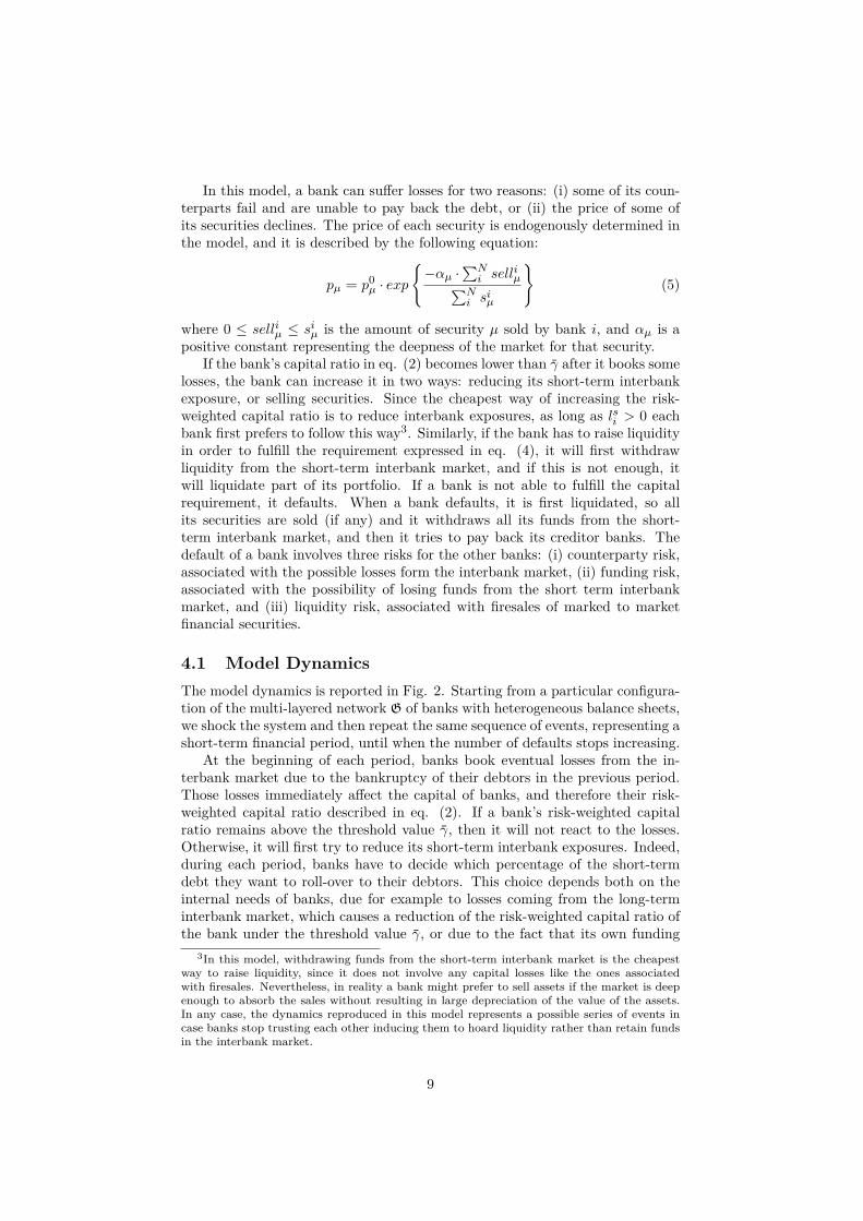
In this model, a bank can suffer losses for two reasons: (i) some of its coun-terparts fail and are unable to pay back the debt, or (ii) the price of some ofits securities declines. The price of each security is endogenously determined inthe model, and it is described by the following equation:

pµ = p0µ · exp

{−αµ ·

∑Ni sell

iµ∑N

i siµ

}(5)

where 0 ≤ selliµ ≤ siµ is the amount of security µ sold by bank i, and αµ is apositive constant representing the deepness of the market for that security.

If the bank’s capital ratio in eq. (2) becomes lower than γ̄ after it books somelosses, the bank can increase it in two ways: reducing its short-term interbankexposure, or selling securities. Since the cheapest way of increasing the risk-weighted capital ratio is to reduce interbank exposures, as long as lsi > 0 eachbank first prefers to follow this way3. Similarly, if the bank has to raise liquidityin order to fulfill the requirement expressed in eq. (4), it will first withdrawliquidity from the short-term interbank market, and if this is not enough, itwill liquidate part of its portfolio. If a bank is not able to fulfill the capitalrequirement, it defaults. When a bank defaults, it is first liquidated, so allits securities are sold (if any) and it withdraws all its funds from the short-term interbank market, and then it tries to pay back its creditor banks. Thedefault of a bank involves three risks for the other banks: (i) counterparty risk,associated with the possible losses form the interbank market, (ii) funding risk,associated with the possibility of losing funds from the short term interbankmarket, and (iii) liquidity risk, associated with firesales of marked to marketfinancial securities.

4.1 Model DynamicsThe model dynamics is reported in Fig. 2. Starting from a particular configura-tion of the multi-layered network G of banks with heterogeneous balance sheets,we shock the system and then repeat the same sequence of events, representing ashort-term financial period, until when the number of defaults stops increasing.

At the beginning of each period, banks book eventual losses from the in-terbank market due to the bankruptcy of their debtors in the previous period.Those losses immediately affect the capital of banks, and therefore their risk-weighted capital ratio described in eq. (2). If a bank’s risk-weighted capitalratio remains above the threshold value γ̄, then it will not react to the losses.Otherwise, it will first try to reduce its short-term interbank exposures. Indeed,during each period, banks have to decide which percentage of the short-termdebt they want to roll-over to their debtors. This choice depends both on theinternal needs of banks, due for example to losses coming from the long-terminterbank market, which causes a reduction of the risk-weighted capital ratio ofthe bank under the threshold value γ̄, or due to the fact that its own funding

3In this model, withdrawing funds from the short-term interbank market is the cheapestway to raise liquidity, since it does not involve any capital losses like the ones associatedwith firesales. Nevertheless, in reality a bank might prefer to sell assets if the market is deepenough to absorb the sales without resulting in large depreciation of the value of the assets.In any case, the dynamics reproduced in this model represents a possible series of events incase banks stop trusting each other inducing them to hoard liquidity rather than retain fundsin the interbank market.

9

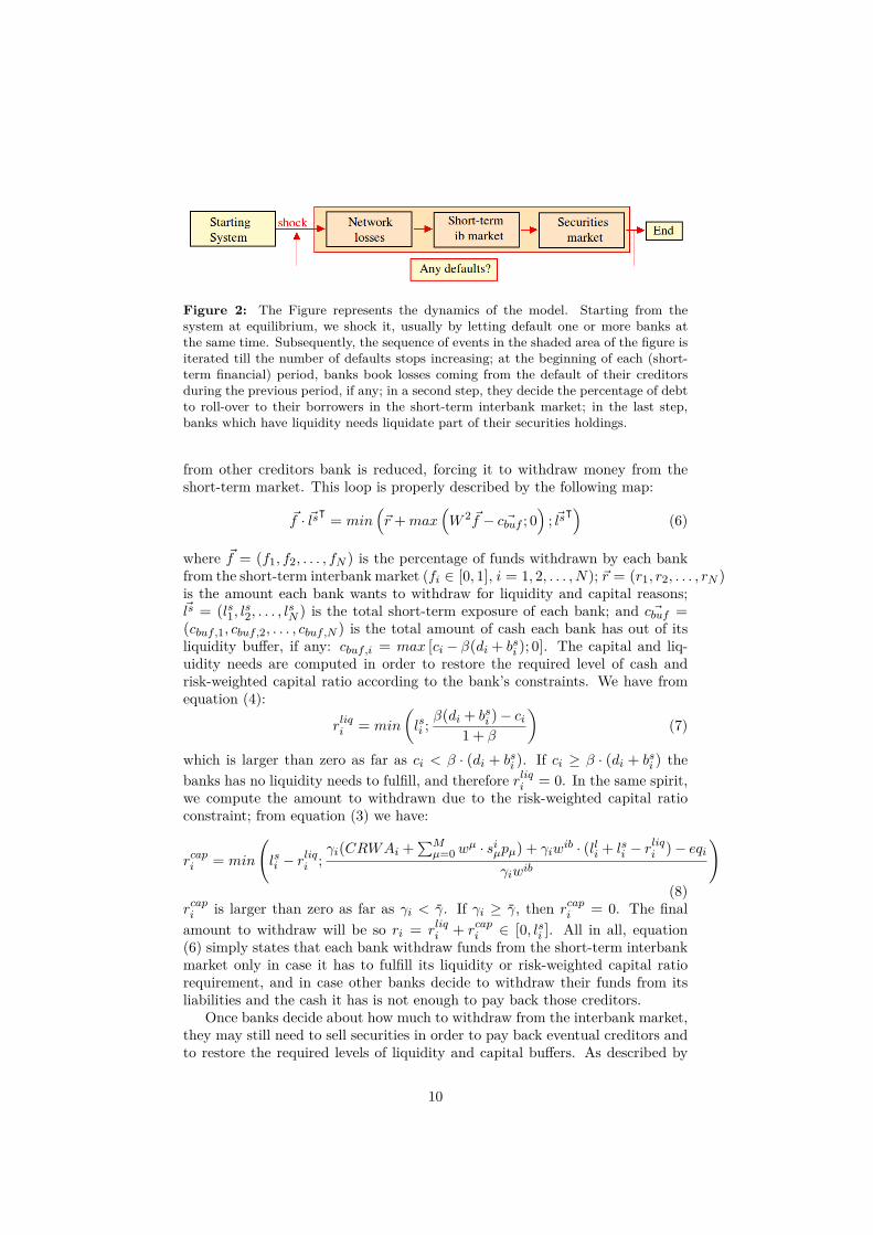
Figure 2: The Figure represents the dynamics of the model. Starting from thesystem at equilibrium, we shock it, usually by letting default one or more banks atthe same time. Subsequently, the sequence of events in the shaded area of the figure isiterated till the number of defaults stops increasing; at the beginning of each (short-term financial) period, banks book losses coming from the default of their creditorsduring the previous period, if any; in a second step, they decide the percentage of debtto roll-over to their borrowers in the short-term interbank market; in the last step,banks which have liquidity needs liquidate part of their securities holdings.

from other creditors bank is reduced, forcing it to withdraw money from theshort-term market. This loop is properly described by the following map:

~f · ~lsᵀ = min(~r+max

(W 2 ~f − ~cbuf ; 0

); ~lsᵀ

)(6)

where ~f = (f1, f2, . . . , fN ) is the percentage of funds withdrawn by each bankfrom the short-term interbank market (fi ∈ [0, 1], i = 1, 2, . . . ,N); ~r = (r1, r2, . . . , rN )is the amount each bank wants to withdraw for liquidity and capital reasons;~ls = (ls1, ls2, . . . , lsN ) is the total short-term exposure of each bank; and ~cbuf =(cbuf ,1, cbuf ,2, . . . , cbuf ,N ) is the total amount of cash each bank has out of itsliquidity buffer, if any: cbuf ,i = max [ci − β(di + bsi ); 0]. The capital and liq-uidity needs are computed in order to restore the required level of cash andrisk-weighted capital ratio according to the bank’s constraints. We have fromequation (4):

rliqi = min

(lsi ;

β(di + bsi )− ci1 + β

)(7)

which is larger than zero as far as ci < β · (di + bsi ). If ci ≥ β · (di + bsi ) thebanks has no liquidity needs to fulfill, and therefore rliqi = 0. In the same spirit,we compute the amount to withdrawn due to the risk-weighted capital ratioconstraint; from equation (3) we have:

rcapi = min

(lsi − r

liqi ;

γi(CRWAi +∑Mµ=0 w

µ · siµpµ) + γiwib · (lli + lsi − r

liqi )− eqi

γiwib

)(8)

rcapi is larger than zero as far as γi < γ̄. If γi ≥ γ̄, then rcapi = 0. The finalamount to withdraw will be so ri = rliqi + rcapi ∈ [0, lsi ]. All in all, equation(6) simply states that each bank withdraw funds from the short-term interbankmarket only in case it has to fulfill its liquidity or risk-weighted capital ratiorequirement, and in case other banks decide to withdraw their funds from itsliabilities and the cash it has is not enough to pay back those creditors.

Once banks decide about how much to withdraw from the interbank market,they may still need to sell securities in order to pay back eventual creditors andto restore the required levels of liquidity and capital buffers. As described by

10

eq. (6), banks first use their available liquidity to pay back creditors, and ifthis is not enough they withdraw funds from the short-term interbank market.In case they still need liquidity, they have to liquidate some securities. We canindicate with Z ∈ RN×M the matrix whose entries Ziµ ≥ 0 indicate how manysecurities of kind µ bank i has to sell in order to fulfill its needs. Since thesecurities prices are adjusting according to eq (5), we use a modified versionof the map introduced by Eisenberg and Noe (2001) in order to compute bothmatrix Z and the clearing vector ~p which resolves the system. We have:

~p = min[~l; Πᵀ · ~p+ ~c+ Z · ~v

](9)

where we denoted with Π the matrix with the relative obligations among banks,that is:

Πij =w2jifj∑j w

2jifj

(10)

The vector ~l represents the total obligations of the banks towards the otherinstitutions, that is:

li =∑j

w2jifj (11)

and ~v is the vector indicating the value of each security, according to eq. (5).In turn, the matrix Z is computed as the sum of three components, which are

the liquidity needs driven by obligations towards other banks in the system, theliquidity needs driven by the requirement expressed in eq. (4), and the liquidityneeds driven by the capital requirement expressed in eq. (3). In more details,they can be formalized as follows: suppose there is only one security in thesystem, the generalization to the case of several securities is then straightaway;in this case, the matrix Z becomes a vector, again composed by three parts; thefirst part is:

Zib = min

[max

[0;~l−~c−Πᵀ · ~p

pµ

];~s]

(12)

where we indicated with ~s = (s1, s2, . . . , sN ) the amount of securities eachbank still have in its portfolio. This is the component driven by the credit linereduction in the short-term interbank market.

The second components is:

Zliq = min

max[0;~c− α(~d+ ~bs)

]pµ

;~s

(13)

This component takes into account for the liquidity requirements of banks.Eventually, there is the component due to the necessity of fulfilling capital

requirements, which is larger than zero if also by withdrawing all their fundsfrom the short-term interbank market they still need to increase their risk-weighted capital ratio:

Zcap = min

wib ~lib +wµpµ − ~eqγ̄

wµ;~s

(14)

11

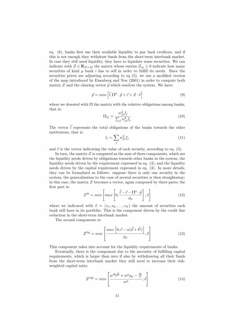
The sum of these three components represents the total amount which ap-pears in eq. (9) : Z = Zib + Zliq + Zcap. The generalization to the case ofmultiple securities is simply derived as follow: each bank tries to sells the firsttype of security in its portfolio; if the bank sell all those securities, it movesto the second type of security, and so on, up to the point when it fulfills itsliquidity needs. Alternatively if its liquidity needs cannot be fulfilled, the bankwill have to sell all its securities.

After the payment vector ~p is computed, banks which are not able to payback their creditors or to fulfill their Risk-Weighted Capital Ratio (hereafterRWCR) are declared in default, they are liquidated and eventual losses aretransmitted through the long and short-term interbank market at the beginningof the next period. The dynamic is repeated till the number of defaults stopsincreasing. It should also be noted here that in our framework a bank candefault for two different reasons: first, it can be unable to fulfill liquidity orcapital requirements, second, it may be illiquid and become unable to pay backits debtors.

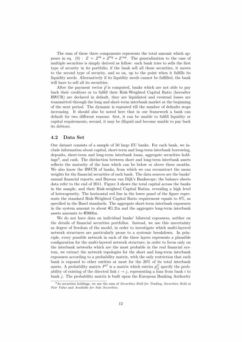
4.2 Data SetOur dataset consists of a sample of 50 large EU banks. For each bank, we in-clude information about capital, short-term and long-term interbank borrowing,deposits, short-term and long-term interbank loans, aggregate securities hold-ings4, and cash. The distinction between short and long-term interbank assetsreflects the maturity of the loan which can be below or above three months.We also know the RWCR of banks, from which we can reconstruct the meanweights for the financial securities of each bank. The data sources are the banks’annual financial reports, and Bureau van Dijk’s Bankscope; the balance sheetsdata refer to the end of 2011. Figure 3 shows the total capital across the banksin the sample, and their Risk-weighted Capital Ratios, revealing a high levelof heterogeneity. The horizontal red line in the lower panel of the figure repre-sents the standard Risk-Weighted Capital Ratio requirement equals to 8%, asspecified in the Basel standards. The aggregate short-term interbank exposuresin the system amount to about e1.2tn and the aggregate long-term interbankassets amounts to e900bn.

We do not have data on individual banks’ bilateral exposures, neither onthe details of financial securities portfolios. Instead, we use this uncertaintyas degree of freedom of the model, in order to investigate which multi-layerednetwork structures are particularly prone to a systemic breakdown. In prin-ciple, every possible network in each of the three layers represents a plausibleconfiguration for the multi-layered network structure; in order to focus only onthe interbank networks which are the most probable in the real financial sys-tem, we extract the network topologies for the short and long-term interbankexposures according to a probability matrix, with the only restriction that eachbank is exposed to other entities at most for the 20% of its total interbankassets. A probability matrix PG is a matrix which entries pGij specify the prob-ability of existing of the directed link i→ j, representing a loan from bank i tobank j. The probability matrix is built upon the European Banking Authority

4As securities holdings, we use the sum of Securities Held for Trading, Securities Held atFair Value and Available for Sale Securities.

12

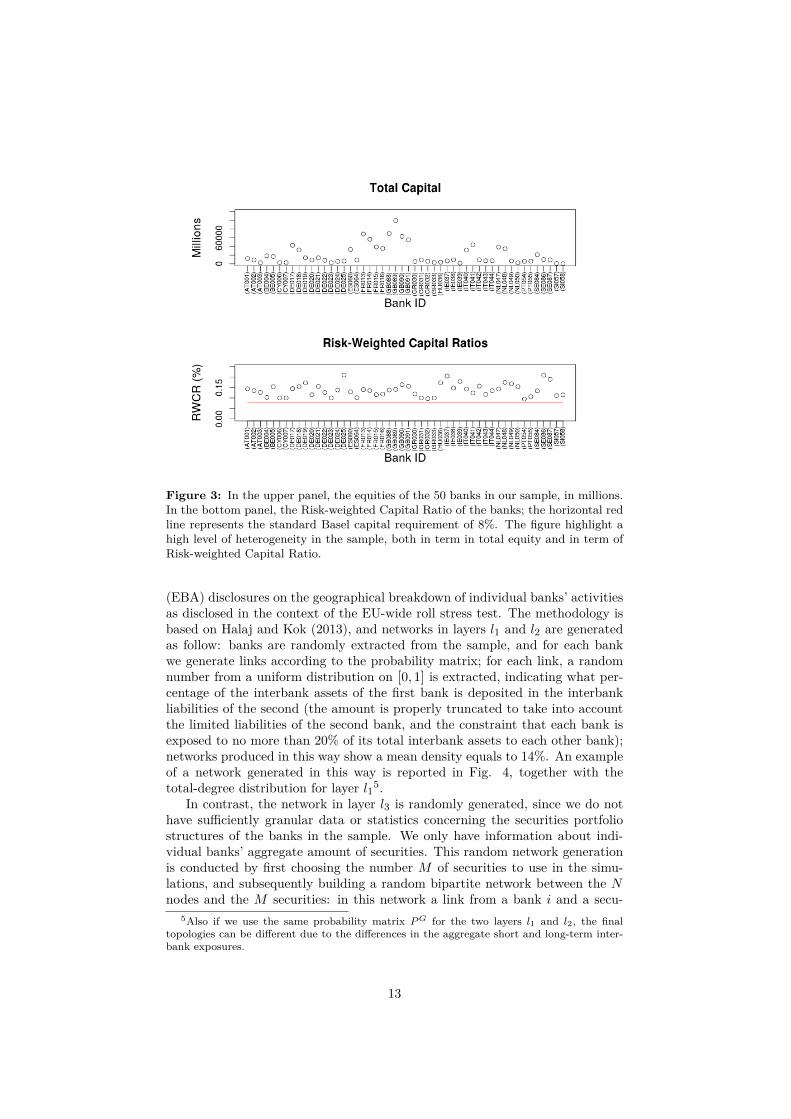
Figure 3: In the upper panel, the equities of the 50 banks in our sample, in millions.In the bottom panel, the Risk-weighted Capital Ratio of the banks; the horizontal redline represents the standard Basel capital requirement of 8%. The figure highlight ahigh level of heterogeneity in the sample, both in term in total equity and in term ofRisk-weighted Capital Ratio.

(EBA) disclosures on the geographical breakdown of individual banks’ activitiesas disclosed in the context of the EU-wide roll stress test. The methodology isbased on Halaj and Kok (2013), and networks in layers l1 and l2 are generatedas follow: banks are randomly extracted from the sample, and for each bankwe generate links according to the probability matrix; for each link, a randomnumber from a uniform distribution on [0, 1] is extracted, indicating what per-centage of the interbank assets of the first bank is deposited in the interbankliabilities of the second (the amount is properly truncated to take into accountthe limited liabilities of the second bank, and the constraint that each bank isexposed to no more than 20% of its total interbank assets to each other bank);networks produced in this way show a mean density equals to 14%. An exampleof a network generated in this way is reported in Fig. 4, together with thetotal-degree distribution for layer l15.

In contrast, the network in layer l3 is randomly generated, since we do nothave sufficiently granular data or statistics concerning the securities portfoliostructures of the banks in the sample. We only have information about indi-vidual banks’ aggregate amount of securities. This random network generationis conducted by first choosing the number M of securities to use in the simu-lations, and subsequently building a random bipartite network between the Nnodes and the M securities: in this network a link from a bank i and a secu-

5Also if we use the same probability matrix PG for the two layers l1 and l2, the finaltopologies can be different due to the differences in the aggregate short and long-term inter-bank exposures.

13

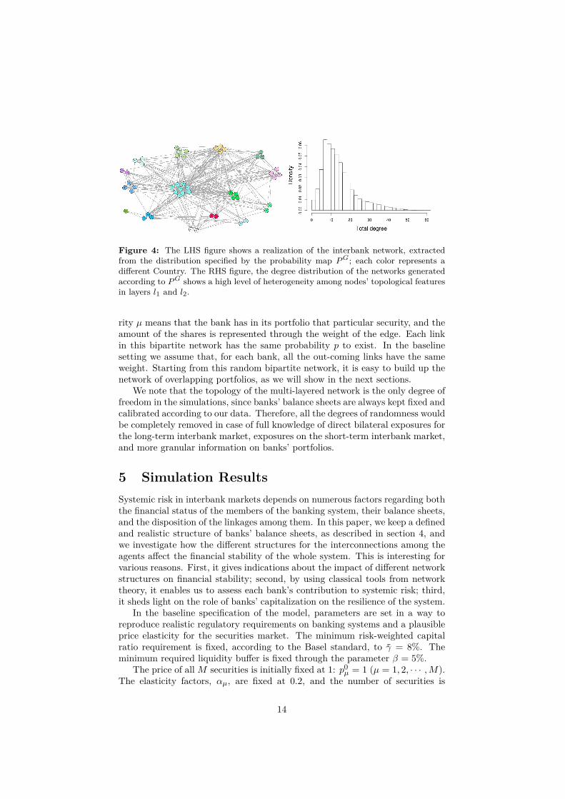
Figure 4: The LHS figure shows a realization of the interbank network, extractedfrom the distribution specified by the probability map P G; each color represents adifferent Country. The RHS figure, the degree distribution of the networks generatedaccording to P G shows a high level of heterogeneity among nodes’ topological featuresin layers l1 and l2.

rity µ means that the bank has in its portfolio that particular security, and theamount of the shares is represented through the weight of the edge. Each linkin this bipartite network has the same probability p to exist. In the baselinesetting we assume that, for each bank, all the out-coming links have the sameweight. Starting from this random bipartite network, it is easy to build up thenetwork of overlapping portfolios, as we will show in the next sections.

We note that the topology of the multi-layered network is the only degree offreedom in the simulations, since banks’ balance sheets are always kept fixed andcalibrated according to our data. Therefore, all the degrees of randomness wouldbe completely removed in case of full knowledge of direct bilateral exposures forthe long-term interbank market, exposures on the short-term interbank market,and more granular information on banks’ portfolios.

5 Simulation ResultsSystemic risk in interbank markets depends on numerous factors regarding boththe financial status of the members of the banking system, their balance sheets,and the disposition of the linkages among them. In this paper, we keep a definedand realistic structure of banks’ balance sheets, as described in section 4, andwe investigate how the different structures for the interconnections among theagents affect the financial stability of the whole system. This is interesting forvarious reasons. First, it gives indications about the impact of different networkstructures on financial stability; second, by using classical tools from networktheory, it enables us to assess each bank’s contribution to systemic risk; third,it sheds light on the role of banks’ capitalization on the resilience of the system.

In the baseline specification of the model, parameters are set in a way toreproduce realistic regulatory requirements on banking systems and a plausibleprice elasticity for the securities market. The minimum risk-weighted capitalratio requirement is fixed, according to the Basel standard, to γ̄ = 8%. Theminimum required liquidity buffer is fixed through the parameter β = 5%.

The price of allM securities is initially fixed at 1: p0µ = 1 (µ = 1, 2, · · · ,M).

The elasticity factors, αµ, are fixed at 0.2, and the number of securities is

14

M = 30. In this way, banks do not have preferences about which securities toliquidate first in case of need, and the bipartite network banks-securities, whichrepresents banks’ securities holdings, is built with a Erdös-Rényi index p = 0.2.We will investigate later how the number of securities and the topology of thenetwork in layer l3 affect the results.

The initial shocks are assumed to derive from the failure of one of the 50banks in the sample. The failure of the bank implies the liquidation of allits securities holdings, the transmission of losses on the long-term interbankmarket, if any, and the withdrawn of all the funds it provides in the short-terminterbank market. The risk for the system hence materializes via the lack of thefunding services provided by the targeted bank, together with the risk of lossestransmitted through the exposure channel and the securities market. How thesystem reacts to this initial shock strongly depends on the topological structureof the underlying multi-layered network.

5.1 Systemically Important BanksThe importance of a bank in a banking system does not depend only on itsfinancial situation. In fact, contagion is a process involving two main steps: thedefault of one or more components of the system, which in turn depends onthe financial situation of the entities, and the propagation of the shock throughinterbank linkages. In this paper, we are interested in this second effect, namelyhow the network structure can affect the stability of the system after an idiosyn-cratic shock hits one of the banks, and part of our task is to determine whichstructures are more prone to financial breakdowns.

A first result from our simulation engine is a test of the impact of each bank’sfailure on the whole system. For this purpose, we first shock one initial bank,we call it bank b0, and then we let the system evolve according to the schemein Fig. 2 up to when the number of defaults stops increasing. The impact ofeach bank on the financial stability of the system is measured through the totalnumber of defaults it produces. This number of defaults is the random variablewe want to estimate the distribution of. In fact, even if the banks’ balancesheets are always the same, including also the aggregate exposures of each banktowards all the others, the degree of randomness left in the structure of thefinancial multi-layered system produces a level of uncertainty on the number ofdefaults following the bankruptcy of bank b06.

In order to highlight the role of each bank in the system, we present thedisentangled effects from the three layers, together with the effects coming fromthe complete multi-layered network’s structure. To this end, we first run thesimulations when all the banks are only connected through the long-term in-terbank market, meaning that the only layers presenting some edges is l1; theonly risk present in this system is therefore the counterparty risk. Then we runthe same simulations with only layer l2 activated, meaning that the only riskpresent in the system is the funding risk7. In the third scenario, we run the

6It should be recalled that when the bank b0 defaults at the beginning of the simulation, itis liquidated, implying that it withdraws all its funds from the short-term interbank market,it sells all its available for sale securities, and it tries to pay back its creditors on the shortand long-term interbank market.

7In those two scenarios, each bank is assumed to have a portfolio which is completelyindependent from all the other banks’ portfolio in the system. Nevertheless, price is still

15

simulations with layer l3 as the only active layer8, representing the case wherethe only risk banks face is liquidity risk. Finally, we present the case where allthe three layers are activated simultaneously.

As a benchmark example, we report the results for one particular bank.The four panels in Fig. 5 show the distributions of the number of defaultsin the four scenarios described above. It is evident that bank DE023 is ingeneral a non-systemic bank, in the sense that in most of the simulations itsbankruptcy does not produce any contagion (in the form of additional bankdefaults). In particular, the contagion through common exposures is almostabsent, as illustrated in the top right panel of the figure9. The red line in thebottom right panel represents the quantitative convolution of the three single-layered network distributions: it basically represents the linear superimpositionof the three effects, and it is interesting to compare it with the distributionfor the total number of defaults in the case of three active layers. As one cansee from the picture, and also from the left-hand side panel in Fig. 6, the twodistributions differ in the way that the three layers working together producemore mass in the tail. In particular, the linear sum of the effects produced by thethree layers separately never increases 9 defaults, while the probability to havemore than 10 defaults in the complete multi-layered network is roughly about5%. This finding clearly highlights the non-linearity in multi-layered systems:the three channels of contagion working together usually produce many moredefaults than the sum of the defaults when the single layers are active separately.

In the right-hand side panel of Fig. 6 one can see the dynamics of thecontagion process when bank DE023 defaults for one specific configuration of themulti-layered network. In particular, the red bold line represents the evolution ofthe number of defaults when all the three layers are working together. The otherlines represent all the possible combinations of the contagion channels. Simplyby eye-balling, it is easy to discern that the sum of the number of defaults inthe single-channel scenarios never reaches the total number of defaults for thewhole system. A deeper examination reveals that this phenomenon is actuallydue to spiral effects: in case only one of the three layers is active, the contagionprocess is dampened (see Fig. 6). Yet when more than one channel of contagionis present, the contagion process is much more probable, and liquidity needs ofone bank can result in a capital reduction of others, which have to increasetheir capital ratio by withdrawing further short-term funds or by liquidatingtheir liquidity portfolio.

Two other interesting examples from the simulation engine are worth noting,where the non-linear nature in which counterparty, funding and liquidity riskcombine each other is much more marked. In Fig. 7, the default of bank DE019is the initial shock inflicted to the system. It is observed that the default of thisdriven by eq. (5), and therefore firesales can still be costly for the banks, also if there are nocontagion effects due to common exposures.

8In this third scenario, all the interbank assets of the institutions in our sample are supposedto be directed to an external node, and all the liabilities in the interbank market are providedby this node, which does not play any other role in our financial simulator, in the sense thatit never withdraws funds and it cannot fail or transmit any losses.

9We are using as measure of contagion the total number of defaults following an initialbankruptcy. Of course, other choices are possible. One could instead use, for example, theaggregate reduction of capital in the system. Also if this measures is not very indicative, sinceit does not specify which banks incurred the losses and if the losses produced defaults, in thatcase also the panel in the top right would produce some non-null results.

16

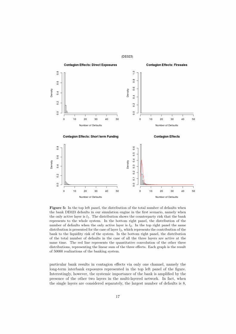
Figure 5: In the top left panel, the distribution of the total number of defaults whenthe bank DE023 defaults in our simulation engine in the first scenario, namely whenthe only active layer is l1. The distribution shows the counterparty risk that the bankrepresents to the whole system. In the bottom right panel, the distribution of thenumber of defaults when the only active layer is l2. In the top right panel the samedistribution is presented for the case of layer l3, which represents the contribution of thebank to the liquidity risk of the system. In the bottom right panel, the distributionof the total number of defaults in the case of all the three layers are active at thesame time. The red line represents the quantitative convolution of the other threedistributions, representing the linear sum of the three effects. Each graph is the resultof 50000 realizations of the banking system.

particular bank results in contagion effects via only one channel, namely thelong-term interbank exposures represented in the top left panel of the figure.Interestingly, however, the systemic importance of the bank is amplified by thepresence of the other two layers in the multi-layered network. In fact, whenthe single layers are considered separately, the largest number of defaults is 8,

17

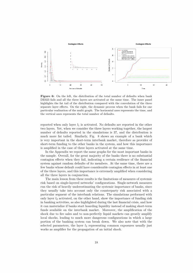
Figure 6: On the left, the distribution of the total number of defaults when bankDE023 fails and all the three layers are activated at the same time. The inner panelhighlights the fat tail of the distribution compared with the convolution of the threeseparate layer effects. On the right, the dynamic process when the bank fails for oneparticular realization of the multi graph. The horizontal axes represents the time, andthe vertical axes represents the total number of defaults.

reported when only layer l1 is activated. No defaults are reported in the othertwo layers. Yet, when we consider the three layers working together, the largestnumber of defaults reported in the simulations is 37, and the distribution ismuch more fat tailed. Similarly, Fig. 8 shows an example of a bank whichis very important in the short-term interbank market, therefore as provider ofshort-term funding to the other banks in the system, and how this importanceis amplified in the case of three layers activated at the same time.

In the Appendix we report the same graphs for the most important banks inthe sample. Overall, for the great majority of the banks there is no substantialcontagion effects when they fail, indicating a certain resilience of the financialsystem against random defaults of its members. At the same time, there are afew banks whose default could have considerable contagion effects in at least oneof the three layers, and this importance is extremely amplified when consideringall the three layers in conjunction.

The main lesson from these results is the limitations of measures of systemicrisk based on single-layered networks’ configurations. Single-network measuresrun the risk of heavily underestimating the systemic importance of banks, sincethey usually take into account only the counterparty risk associated with aparticular segment of the interbank relations. The simulations performed withonly layer l2 activated, on the other hand, show the importance of funding riskin banking activities, as also highlighted during the last financial crisis, and howit can materialize if banks start hoarding liquidity instead of making short-termfunds available on the interbank market. Moreover, the amplification of theshock due to fire sales and to non-perfectly liquid markets can greatly amplifylocal shocks, leading to much more dangerous configurations in which a largeportion of the banking system can break down. We also note that with theselected parameters, the layer l3 representing common exposures usually justworks as amplifier for the propagation of an initial shock.

18

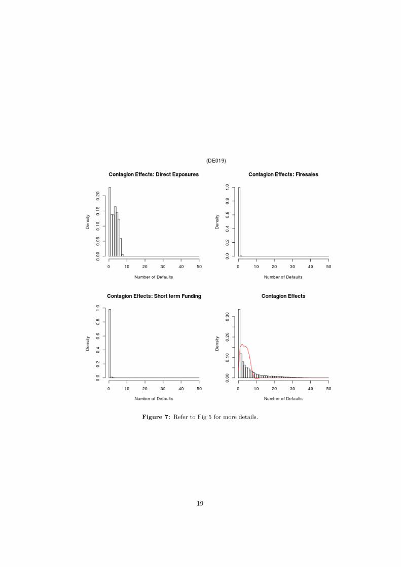
Figure 7: Refer to Fig 5 for more details.

19

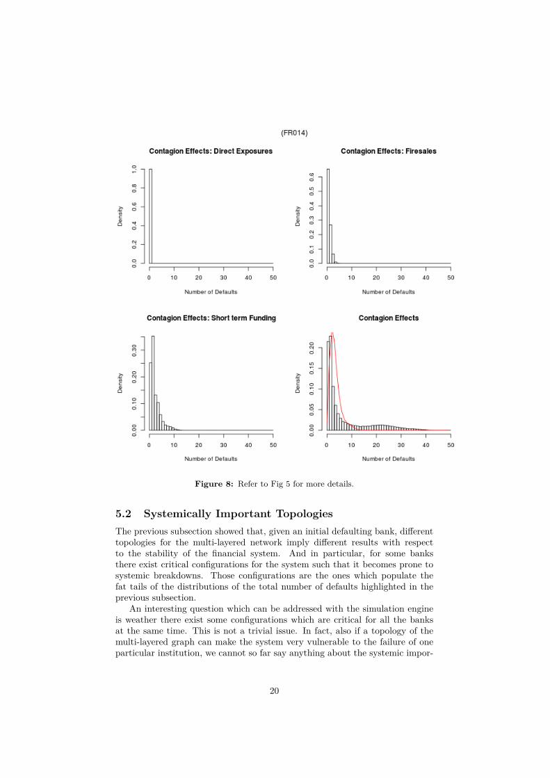
Figure 8: Refer to Fig 5 for more details.

5.2 Systemically Important TopologiesThe previous subsection showed that, given an initial defaulting bank, differenttopologies for the multi-layered network imply different results with respectto the stability of the financial system. And in particular, for some banksthere exist critical configurations for the system such that it becomes prone tosystemic breakdowns. Those configurations are the ones which populate thefat tails of the distributions of the total number of defaults highlighted in theprevious subsection.

An interesting question which can be addressed with the simulation engineis weather there exist some configurations which are critical for all the banksat the same time. This is not a trivial issue. In fact, also if a topology of themulti-layered graph can make the system very vulnerable to the failure of oneparticular institution, we cannot so far say anything about the systemic impor-

20

tance of the other banks in exactly the same network structure. In case a veryimportant bank for the system in terms of the financial services it provides tothe other banks, assumes a central position in the network structure, systemicrisk is high, since the bankruptcy of this bank can create contagion effects whichaffects a large number of other financial institutions. If substantial contagionoccurs only in some of the simulated network structures we generate in oursimulations, it means that, in those cases, the idiosyncratic risk assumed bythe defaulting bank was badly distributed among the other institutions in thesystem. We therefore speak about systemic risk, and systemically important in-stitutions. Moreover, the possibility that more large banks become systemicallyimportant at the same time is a much riskier situation for the entire system.Given the probability matrix PG, we are interested in investigating the possi-bility of existence of systemically important topologies; formally, given a certainmulti-layered graph G, we can compute the systemic risk associated with thestructure as follow:

RG =

∑Ni=1 d(i)

N(15)

where we indicate with d(i) the number of defaults caused by the bankruptcyof bank i, computed as the result of our simulation engine.

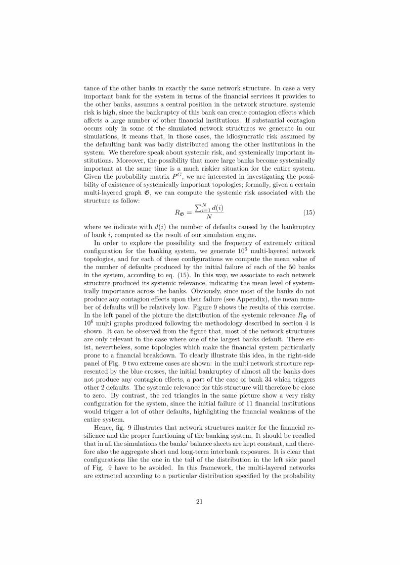
In order to explore the possibility and the frequency of extremely criticalconfiguration for the banking system, we generate 106 multi-layered networktopologies, and for each of these configurations we compute the mean value ofthe number of defaults produced by the initial failure of each of the 50 banksin the system, according to eq. (15). In this way, we associate to each networkstructure produced its systemic relevance, indicating the mean level of system-ically importance across the banks. Obviously, since most of the banks do notproduce any contagion effects upon their failure (see Appendix), the mean num-ber of defaults will be relatively low. Figure 9 shows the results of this exercise.In the left panel of the picture the distribution of the systemic relevance RG of106 multi graphs produced following the methodology described in section 4 isshown. It can be observed from the figure that, most of the network structuresare only relevant in the case where one of the largest banks default. There ex-ist, nevertheless, some topologies which make the financial system particularlyprone to a financial breakdown. To clearly illustrate this idea, in the right-sidepanel of Fig. 9 two extreme cases are shown: in the multi network structure rep-resented by the blue crosses, the initial bankruptcy of almost all the banks doesnot produce any contagion effects, a part of the case of bank 34 which triggersother 2 defaults. The systemic relevance for this structure will therefore be closeto zero. By contrast, the red triangles in the same picture show a very riskyconfiguration for the system, since the initial failure of 11 financial institutionswould trigger a lot of other defaults, highlighting the financial weakness of theentire system.

Hence, fig. 9 illustrates that network structures matter for the financial re-silience and the proper functioning of the banking system. It should be recalledthat in all the simulations the banks’ balance sheets are kept constant, and there-fore also the aggregate short and long-term interbank exposures. It is clear thatconfigurations like the one in the tail of the distribution in the left side panelof Fig. 9 have to be avoided. In this framework, the multi-layered networksare extracted according to a particular distribution specified by the probability

21

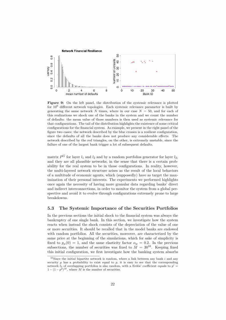
Figure 9: On the left panel, the distribution of the systemic relevance is plottedfor 106 different network topologies. Each systemic relevance parameter is built bygenerating the same network N times, where in our case N = 50, and for each ofthis realizations we shock one of the banks in the system and we count the numberof defaults: the mean value of those numbers is then used as systemic relevance forthat configurations. The tail of the distribution highlights the existence of some criticalconfigurations for the financial system. As example, we present in the right panel of thefigure two cases: the network described by the blue crosses is a resilient configuration,since the defaults of all the banks does not produce any considerable effects. Thenetwork described by the red triangles, on the other, is extremely unstable, since thefailure of one of the largest bank trigger a lot of subsequent defaults.

matrix PG for layer l1 and l2 and by a random portfolios generator for layer l3,and they are all plausible networks, in the sense that there is a certain prob-ability for the real system to be in those configurations. In reality, however,the multi-layered network structure arises as the result of the local behaviorsof a multitude of economic agents, which (supposedly) have as target the max-imization of their personal interests. The experiments we performed highlightsonce again the necessity of having more granular data regarding banks’ directand indirect interconnections, in order to monitor the system from a global per-spective and avoid it to evolve through configurations extremely prone to largebreakdowns.

5.3 The Systemic Importance of the Securities PortfoliosIn the previous sections the initial shock to the financial system was always thebankruptcy of one single bank. In this section, we investigate how the systemreacts when instead the shock consists of the depreciation of the value of oneor more securities. It should be recalled that in the model banks are endowedwith random portfolios. All the securities, moreover, are characterized by thesame price at the beginning of the simulations, which for sake of simplicity isfixed to pµ(0) = 1, and the same elasticity factor αµ = 0.2. In the previoussubsections, the number of securities was fixed to M = 3010. Keeping fixedthis initial configuration, we first investigate how the banking system absorbs

10Since the initial bipartite network is random, where a link between any bank i and anysecurity µ has a probability to exist equal to p, it is easy to see that the correspondingnetwork l3 of overlapping portfolios is also random, with a Erdös’ coefficient equals to p′ =1 − (1 − p2)M , where M is the number of securities.

22

a price reduction of one or more securities. Fig. 10 shows the results. Inthe left side panels the number of defaults following a certain percentage ofreduction of the securities’ price is shown, respectively when the price reductionaffects only one security (top left panel), two securities (top right panel), threesecurities (bottom left panel) and ten securities (bottom right panel). In each ofthe graphs are reported the mean number of defaults corresponding to differentshock sizes, where the solid line represents the situation when all the three layersare activated, while the dashed line represents the situation when the only activelayer is l3. It is observed that if banks were completely independent from eachother in the layers l1 and l2, there would be very few defaults, especially forprice shocks which are not abnormally large11. Consider, for example, the casewhen 10 securities are shocked at the same time by reducing their value of 15%.Without any other connections among banks apart from the common exposures,the mean number of defaults is around 7. Meanwhile this number drasticallyincreases to 38 if banks are also connected through layers l1 and l2. We notethat since all the securities have the initial same price, and are all characterizedby the same elasticity factor, in this random portfolio scenario it does not playa role which securities are shocked, since the effects are averaged out whenthe number of simulations is large enough. Eventually, as one can see fromthe figure, for values of the shock smaller than 5% no defaults are observed,indicating an adequate capital buffer level for small losses in banks’ securitiesportfolios.

On the right-side panel of Fig. 10 we report the tails of the distributions ofthe number of defaults for a shock to the securities equal to 15%, for the casesof one, two, three and ten initial shocked securities respectively. The blue areashighlighted in the graphs represent the last fifth quantile of the distributions. Inthe cases of one, two and three shocked securities, the great part of the mass ofthese distributions is concentrated in values close to zero, highlighting a consid-erable financial resilience of the banking system for random assets depreciations.Nevertheless, one can see in the graphs that, also in the scenario of one securityshocked by 15% of its initial value, the shock can be amplified to destroy a largepart of the banking system12. These findings highlight that also if the initialshock derives from a depreciation of the mark-to-market banks’ portfolios, themulti-layered network structure is playing the crucial role of shock amplifier.

A particular aspect related to the banks’ portfolio structures should be high-lighted. In all the previous results, the securities portfolios were built accordingto the random algorithm described in section 4.2. It should be noted however,that since all the securities in our framework are equivalent, banks maximizetheir utilities by simply allocating their funds in equal measure in all the possi-ble available securities. In this configuration the system results in a maximumdegree of overlap of banks’ portfolios, which implies a fully connected (i.e. com-plete) network in the layer l3. The diametric opposite of this configurationhappens when banks invest all in different securities, which translates in an

11We report in the graphs all the possible values for a shock, so from 0% to 100% of reductionof the asset’s value; of course, this is only an illustrative simulation exercise, since in realitydepreciations larger than 20% are extremely rare.

12We note that those fat tails disappear as far as the layers l1 and l2 are deactivated. Wedo not report here here also those distributions, but one can see from Fig. 10 that the meanvalues of the number of defaults is exactly zero for shocks equal to 15% (dashed lines in theleft side panels), a part of the case when ten securities are shocked at the same time.

23

Figure 10: On the left side of the figure, the four panels show the number of defaultswhen one, two three and ten securities are shocked; the solid lines represent the numberof defaults when all the three layers are active at the same time, while the dashed linesrepresents the same results when only the layer l3 is activated (firesales contagioneffects). On the right side, the tails of the distributions of the total number of defaultsare reported, when the percentage of securities’ reduction is equal to 15%; results arehere reported for the case of one, two, three and ten initially shocked securities. Theblue areas highlighted represent the last fifth quantile of the distributions.

empty network in the layer l3. In order to illustrate the impact that the degreeof overlapping portfolios has on systemic risk, we use now a number of securi-ties M equal to N , the number of banks. This allows for comparing situationsranging from banks having maximum overlapping portfolios (precisely, when allthe banks equally share their funds among all the possible M securities), tosituations where banks invest their funds in only one security and there are nocommon exposures among them. The results of this exercise are shown in figure11. We assume that the shock is a reduction of the value of all the M securitiesin the system, respectively of 5% (black line), 7% (red line), 10% (blue line)and 15% (green line). In this way, for a given shock size, all the banks have tobook the same losses (in percentage points) in all the portfolios’ configurationwe examine. The horizontal axes of the graph reports the number ns of secu-rities each bank is investing in, and the portfolios are built in a way to alwaysminimize the degree of overlap among different banks. When ns is equal toone, each bank has only one security in its portfolios, each different from all theothers (so there is a correspondence one-to-one between the N banks and theM = N securities in the system). When ns is equal to N , each bank invest itsfunds in all the possible securities, and all the banks have the same portfoliostructure. It is interesting to note that moving along the horizontal axes fromleft to right maximizes banks’ portfolio diversification (and hence reduces theirvulnerability to idiosyncratic risk) but at the same time minimizes financialstability (it maximizes the number of defaults, and therefore, roughly speaking,the systemic risk). Our model highlights the interesting duality between maxi-mization of banks’ utility and minimization of systemic risk, a concept alreadyhighlighted in Beale et al (2011) who argue that banks’ portfolios optimizationcan lead to higher level of systemic risk, thereby emphasizing the necessity tosupervise systemic risk from a more global perspective13.

13See also Tasca and Battiston (2012) for similar fundings.

24

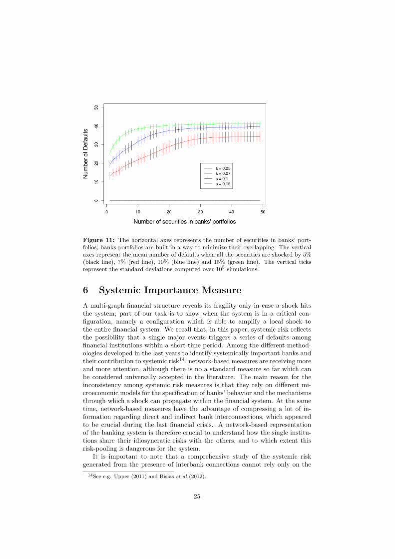
Figure 11: The horizontal axes represents the number of securities in banks’ port-folios; banks portfolios are built in a way to minimize their overlapping. The verticalaxes represent the mean number of defaults when all the securities are shocked by 5%(black line), 7% (red line), 10% (blue line) and 15% (green line). The vertical ticksrepresent the standard deviations computed over 105 simulations.

6 Systemic Importance MeasureA multi-graph financial structure reveals its fragility only in case a shock hitsthe system; part of our task is to show when the system is in a critical con-figuration, namely a configuration which is able to amplify a local shock tothe entire financial system. We recall that, in this paper, systemic risk reflectsthe possibility that a single major events triggers a series of defaults amongfinancial institutions within a short time period. Among the different method-ologies developed in the last years to identify systemically important banks andtheir contribution to systemic risk14, network-based measures are receiving moreand more attention, although there is no a standard measure so far which canbe considered universally accepted in the literature. The main reason for theinconsistency among systemic risk measures is that they rely on different mi-croeconomic models for the specification of banks’ behavior and the mechanismsthrough which a shock can propagate within the financial system. At the sametime, network-based measures have the advantage of compressing a lot of in-formation regarding direct and indirect bank interconnections, which appearedto be crucial during the last financial crisis. A network-based representationof the banking system is therefore crucial to understand how the single institu-tions share their idiosyncratic risks with the others, and to which extent thisrisk-pooling is dangerous for the system.

It is important to note that a comprehensive study of the systemic riskgenerated from the presence of interbank connections cannot rely only on the

14See e.g. Upper (2011) and Bisias et al (2012).

25

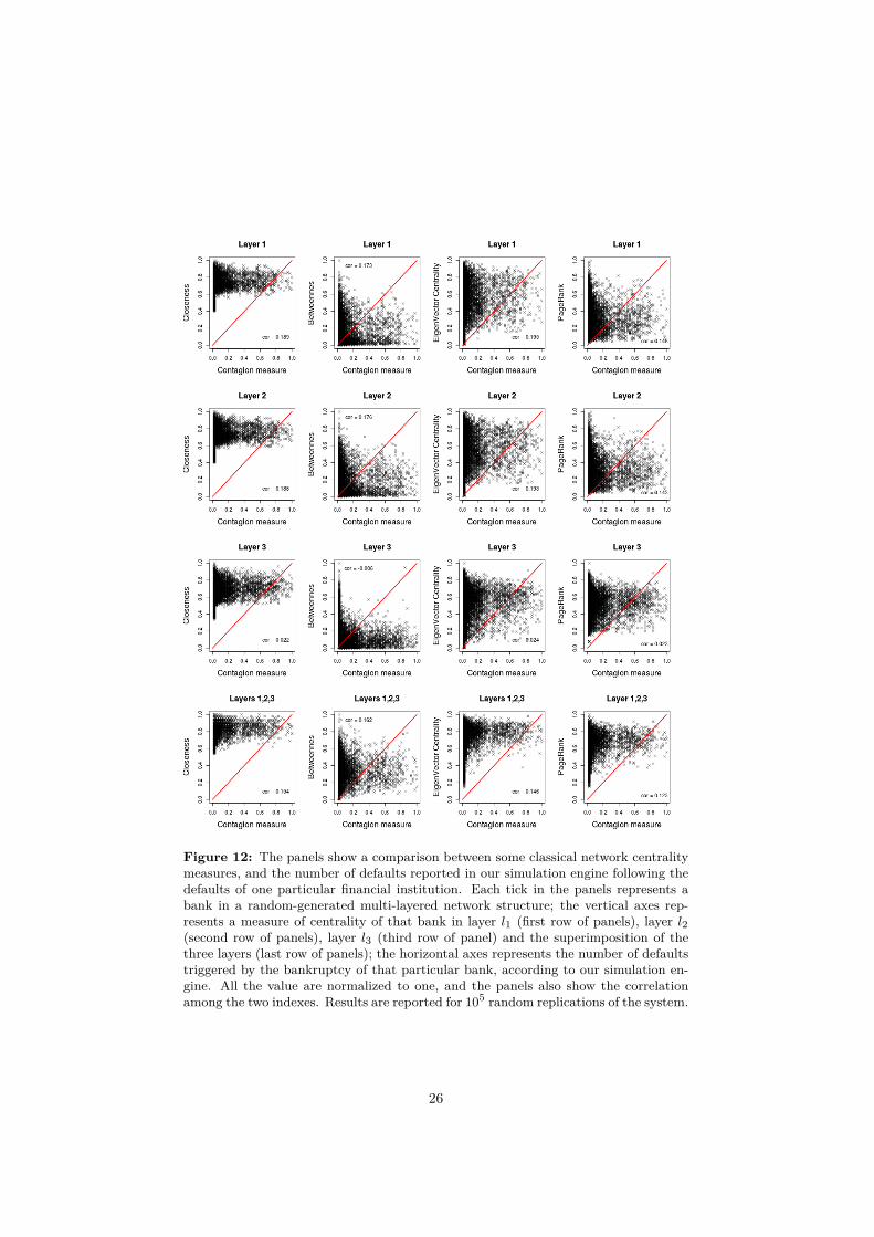
Figure 12: The panels show a comparison between some classical network centralitymeasures, and the number of defaults reported in our simulation engine following thedefaults of one particular financial institution. Each tick in the panels represents abank in a random-generated multi-layered network structure; the vertical axes rep-resents a measure of centrality of that bank in layer l1 (first row of panels), layer l2(second row of panels), layer l3 (third row of panel) and the superimposition of thethree layers (last row of panels); the horizontal axes represents the number of defaultstriggered by the bankruptcy of that particular bank, according to our simulation en-gine. All the value are normalized to one, and the panels also show the correlationamong the two indexes. Results are reported for 105 random replications of the system.

26

network structure of the financial system. The interconnections in an interbankmarket provide a way for banks to pool the unavoidable risks linked to theiractivities, and the interbank market should in principle play a stabilizing rolefor the banking system. A bank which is very connected to a major part of theothers can have a crucial positive role in this scenario if its level of capitalizationis large enough, as it can be able to absorb the local shocks of its neighbors. Sucha bank will be considered as central in terms of spillover potential to other partof the system, but from the economic point of view its presence is beneficial forthe system, since it reduces idiosyncratic risks of other institutions. Figure 12clearly illustrates this notion. The panels in the figure represents a comparisonbetween some classical network centrality measures and the number of defaultsreported in our simulation engine following the bankruptcy of one bank. Thenumber of defaults can be used as a proxy for the systemic importance of abank in the system. Since we are dealing with a multi-layered framework, wecompute four different centrality measures (which are closeness, betweennes,eigenvector centrality and PageRank) for all the three layers separately, andthe same measures when the three layers are projected in a single one. As canbe seen from the panels, there is basically no correlation among those networkmeasures and the number of defaults we obtain from our simulations. Thisresult highlights the necessity to develop more sophisticated measures to assesthe systemic contribution of each institution to the financial system, and thosemeasures have to take into account the articulated internal structure of the nodesin the network (in other words, banks’ balance sheets) as well as the differentmechanisms of contagion and risk-sharing present in the banking system.

This notwithstanding, considering only banks’ balance sheets information toassess the level of systemic risk in the banking sector is extremely restrictive.Prior to the recent financial crisis micro-prudential supervision was based onthe notion that it was sufficient to ensure the stability of the banking sectorto require institutions to have operate with an adequate level of capitalization.The recent financial crisis, if anything, revealed that focusing only on individualbanks’ soundness is a necessary but not sufficient condition for safeguardingthe financial system. In fact, as we will show later, the risk-pooling mechanism,which is at the core of an interbank market, can increase the chances of multiplefailures to occur following an initial shock. Since the process of contagion amongfinancial institutions, as we already highlighted, is composed of two parts, whichare an initial triggering events (for example the failure of one single institution),and the propagation of losses and distress in the financial system, the extent towhich a local shock can propagate and be amplified from bank to bank greatlydepends also on the structure of the banking system as a whole. To illustratethis point, figure 13 shows a comparison between some balance sheet-relatedquantities and the number of defaults following the bankruptcy of a single insti-tution. The figure shows that classical quantities like banks’ total assets, totalinterbank liabilities, total interbank assets and risk-weighted capital ratios donot necessarily provide useful information regarding the systemic importance ofthe bank, as measured by the number of defaults its bankruptcy can trigger.In particular, one can see from the picture that the failure of small-sized banksusually does not trigger too many other defaults. On the other hand, regardinglarge-sized banks we find mixed results in the sense that some of them triggerdomino effects, while others do not. Eventually, the last panel on the right-handside shows that there is no link between the banks risk-weighted capital ratios

27

and their systemic importance.To account for the fact that neither classical centrality measures nor bal-

ance sheet indicators are sufficient for assessing the systemic importance of aninstitution, the next subsection introduces an algorithm to derive the systemiccontribution of each bank to the financial system. The framework will takeinto account both network and balance sheets information, with the final aimof (i) reproducing the results we obtained with the simulation engine; and (ii)visualizing the network structure in a way to highlight how the idiosyncraticrisk of each bank is distributed among the other institutions, and when thisrisk-sharing brings the system to an unstable configuration.

6.1 The aggregation algorithmThe algorithm we propose in this section to study the multi-layered financialnetwork is based on the concept of critical link. In each of the three layers weintroduced, a link starting from node i and pointing to node j is said to becritical if the bankruptcy of bank i results in the bankruptcy of bank j. Wenote immediately that, without critical links in the three layers, no contagioneffect is possible, although losses can be transmitted to the direct neighbors ofthe failed bank. In fact, in case the default of a single bank does not imply anyother failures, the direct and indirect counterparties of that bank were assumingan acceptable amount of risk with respect to their own capital buffer, and wespeak about counterparty risk (or liquidity risk) but not about systemic risk.We can distinguish the conditions for a link to be critical in the three differentlayers15:

• Layer l1: given the matrixW 1 whose entries represent the long-term directexposures among banks, there exists a critical link in layer l1 between twobanks i and j if:

W 1ji ·LGDi >

eqj − γ̄[RWEAj +

∑Mµ=0 pµw

µsjµ +wibllj

]1− γ̄wib (16)

Despite the complicated form of eq. (16), its meaning is simple: a criticallink between nodes i and j exists if node j is not able to absorb thelosses transmitted in case of the defaults of node i. In the above equationwe introduce the losses-given-default (LGD) of bank i, computed as anestimation of the percentage of loans that bank i is not able to repay incase of its default16. We note that the use of LGD is fundamental in orderto replicate a more realistic scenario in the simulations, and the quality ofits estimation depends on the available data.

15The computation of the thresholds necessary to identify critical links represents the trickypart of the algorithm. In fact, a part of layer l1 for which one can easily compute the maximumlosses each bank can absorb without going below the capital requirements, for the other layersapproximations are necessary.

16In our framework, this amount to:

LGDi = 1 −min

[max

[ci +

∑M

µ=0 siµpµ + lsi − bsi

lli; 0

]; 1

](17)

Of course, better calibrations are possible depending on data availability and the dynamicsused in the model.

28

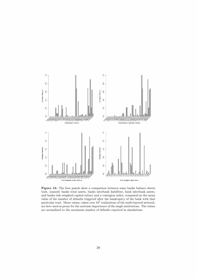
Figure 13: The four panels show a comparison between some banks balance sheetstrait, (namely banks total assets, banks interbank liabilities, bank interbank assets,and banks risk weighted capital ratios) and a contagion index, computed as the meanvalue of the number of defaults triggered after the bankruptcy of the bank with thatparticular trait. Mean values, taken over 105 realizations of the multi-layered network,are here used as proxy for the systemic importance of the single institutions. The valuesare normalized to the maximum number of defaults reported in simulations.

29

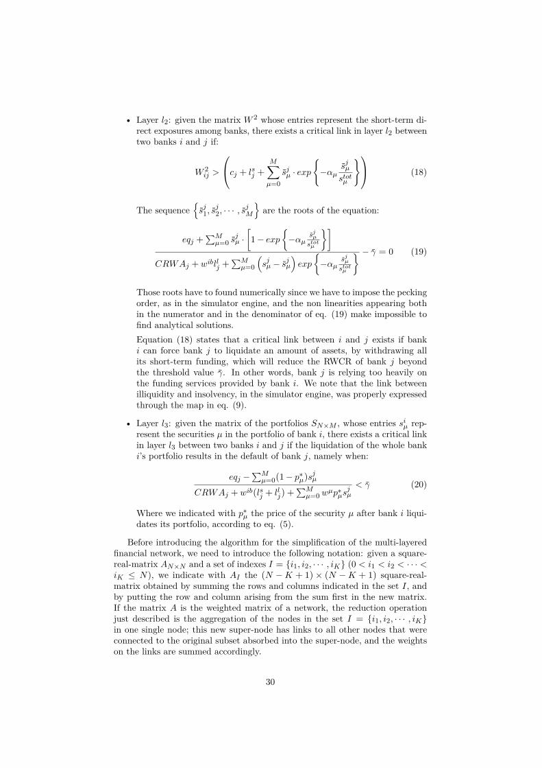
• Layer l2: given the matrix W 2 whose entries represent the short-term di-rect exposures among banks, there exists a critical link in layer l2 betweentwo banks i and j if:

W 2ij >

cj + lsj +M∑µ=0

s̄jµ · exp

{−αµ

s̄jµstotµ

} (18)

The sequence{s̄j1, s̄j2, · · · , s̄jM

}are the roots of the equation:

eqj +∑Mµ=0 s̄

jµ ·[1− exp

{−αµ

s̄jµstotµ

}]CRWAj +wibllj +

∑Mµ=0

(sjµ − s̄jµ

)exp

{−αµ

s̄jµstotµ

} − γ̄ = 0 (19)

Those roots have to found numerically since we have to impose the peckingorder, as in the simulator engine, and the non linearities appearing bothin the numerator and in the denominator of eq. (19) make impossible tofind analytical solutions.Equation (18) states that a critical link between i and j exists if banki can force bank j to liquidate an amount of assets, by withdrawing allits short-term funding, which will reduce the RWCR of bank j beyondthe threshold value γ̄. In other words, bank j is relying too heavily onthe funding services provided by bank i. We note that the link betweenilliquidity and insolvency, in the simulator engine, was properly expressedthrough the map in eq. (9).

• Layer l3: given the matrix of the portfolios SN×M , whose entries siµ rep-resent the securities µ in the portfolio of bank i, there exists a critical linkin layer l3 between two banks i and j if the liquidation of the whole banki’s portfolio results in the default of bank j, namely when:

eqj −∑Mµ=0(1− p∗

µ)sjµ

CRWAj +wib(lsj + llj) +∑Mµ=0 w

µp∗µsjµ

< γ̄ (20)

Where we indicated with p∗µ the price of the security µ after bank i liqui-

dates its portfolio, according to eq. (5).

Before introducing the algorithm for the simplification of the multi-layeredfinancial network, we need to introduce the following notation: given a square-real-matrix AN×N and a set of indexes I = {i1, i2, · · · , iK} (0 < i1 < i2 < · · · <iK ≤ N), we indicate with AI the (N −K + 1) × (N −K + 1) square-real-matrix obtained by summing the rows and columns indicated in the set I, andby putting the row and column arising from the sum first in the new matrix.If the matrix A is the weighted matrix of a network, the reduction operationjust described is the aggregation of the nodes in the set I = {i1, i2, · · · , iK}in one single node; this new super-node has links to all other nodes that wereconnected to the original subset absorbed into the super-node, and the weightson the links are summed accordingly.

30

We can finally introduce the aggregation algorithm for the simplification of amulti-layered financial network. We start with a multi-layered structure G andan initial bank b0 for which we want to compute its systemic importance. Inthe first step, s = 0, we consider the node b0 as the only one in the super-node,and in each step s = 1, 2, · · · we perform the following operations:

1. We build up the matrices W 1Is−1

, W 2Is−1

and W 3Is−1

, where Is−1 are thenodes belonging to the super-node the step before. We note that this isequivalent to introduce a new bank in the system, instead of the banks inthe set Is−1, whose balance sheet is the aggregation of the K suppressedbanks’ balance sheets, and whose links are the aggregation of the in-comingand out-coming links of the nodes in Is−1.

2. We identify the critical links in each of the three layers l1, l2 and l3 andwe build up three new matrices A1

s, A2s and A3

s which entries are:

Als,ij =

{1 if there is a critical link from i to j in layer l0 otherwise

3. We find the directed tree in the unweighted, directed network charac-terized by the adjacency matrix As = A1

s + A2s + A3

s starting from thesuper-node; the nodes belonging to this tree will constitute the set Is,while its edges are recorded in the set Cs.

The algorithm ends when the size of the super-node stops increasing andit happens in at most N steps, since in the worst case each node is absorbedin the super-node in a different step. The first output of the algorithm is aseries of sets of nodes Is (s = 1, 2, · · · ) which can be used to extremely sim-plify the network structure. In fact, nodes absorbed in the super-node in steps are all characterized by the following property: they will fail if all the nodesbelonging to the set Is−1 fail simultaneously, but not if any single node in Is−1fails separately. The second output of the algorithm is the series Cs of linksbelonging to the spanning trees starting from the super-nodes. This series ofcritical links helps us in the identification of critical paths in the system, namelymultidimensional paths which can bring the losses from one node in the networkto a remote region of the same network. A multidimensional critical path hasactually a meaning which is deeper than only being a channel for the transmis-sion of losses through the financial system. The presence of multidimensionalpaths in interbank network represents a way of risk sharing that goes beyond theknowledge of the single banks. The idiosyncratic risk of one single institution isshared not only with its direct counterparties, which are aware of the risk taken,but also with other players not directly connected to the institution, and whichcannot be fully conscious of the risk-transfer represented by the critical paths inthe network. Without a full knowledge of the multi-layered network structureno banks can really estimate its exposure to the idiosyncratic risk of the otherbanks. This is illustrated in the following subsection where we shows how theaggregation algorithm can be used to identify systemic important banks.

6.2 ResultsTo better clarify the working and the outputs of the aggregation algorithm,we analyze one particular scenario, and we show how it is possible to simplify

31

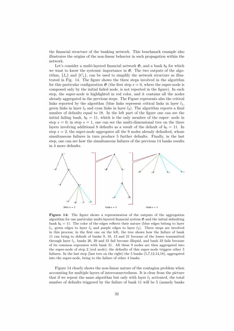
the financial structure of the banking network. This benchmark example alsoillustrates the origins of the non-linear behavior in such propagation within thenetwork.

Let’s consider a multi-layered financial network G, and a bank b0 for whichwe want to know the systemic importance in G. The two outputs of the algo-rithm, {Is} and {Cs}, can be used to simplify the network structure as illus-trated in Fig. 14. The figure shows the three steps involved in the algorithmfor this particular configuration G (the first step s = 0, where the super-node iscomposed only by the initial failed node, is not reported in the figure). In eachstep, the super-node is highlighted in red color, and it contains all the nodesalready aggregated in the previous steps. The Figure represents also the criticallinks reported by the algorithm (blue links represent critical links in layer l1,green links in layer l2 and cyan links in layer l3). The algorithm reports a finalnumber of defaults equal to 18. In the left part of the figure one can see theinitial failing bank, b0 = 11, which is the only member of the super- node instep s = 0; in step s = 1, one can see the multi-dimensional tree on the threelayers involving additional 8 defaults as a result of the default of b0 = 11. Instep s = 2, the super-node aggregates all the 9 nodes already defaulted, whosesimultaneous failures in turn produce 5 further defaults. Finally, in the laststep, one can see how the simultaneous failures of the previous 14 banks resultsin 4 more defaults.

Figure 14: The figure shows a representation of the outputs of the aggregationalgorithm for one particular multi-layered financial system G and the initial defaultingbank b0 = 11. The color of the edges reflects their nature (blue edges belong to layerl1, green edges to layer l2 and purple edges to layer l3). Three steps are involvedin this process; in the first one on the left, the tree shows how the failure of bank11 can bring to default of banks 9, 10, 13 and 21 because of the losses transmittedthrough layer l1, banks 26, 29 and 31 fail become illiquid, and bank 33 fails becauseof its common exposures with bank 21. All these 9 nodes are then aggregated intothe super-node of step 2 (red node); the defaults of this super-node triggers other 5failures. In the last step (last tree on the right) the 5 banks (5,7,12,14,18), aggregatedinto the super-node, bring to the failure of other 4 banks.

Figure 14 clearly shows the non-linear nature of the contagion problem whenaccounting for multiple layers of interconnectedness. It is clear from the picturethat if we repeat the same algorithm but only with layer l1 activated, the totalnumber of defaults triggered by the failure of bank 11 will be 5 (namely banks

32

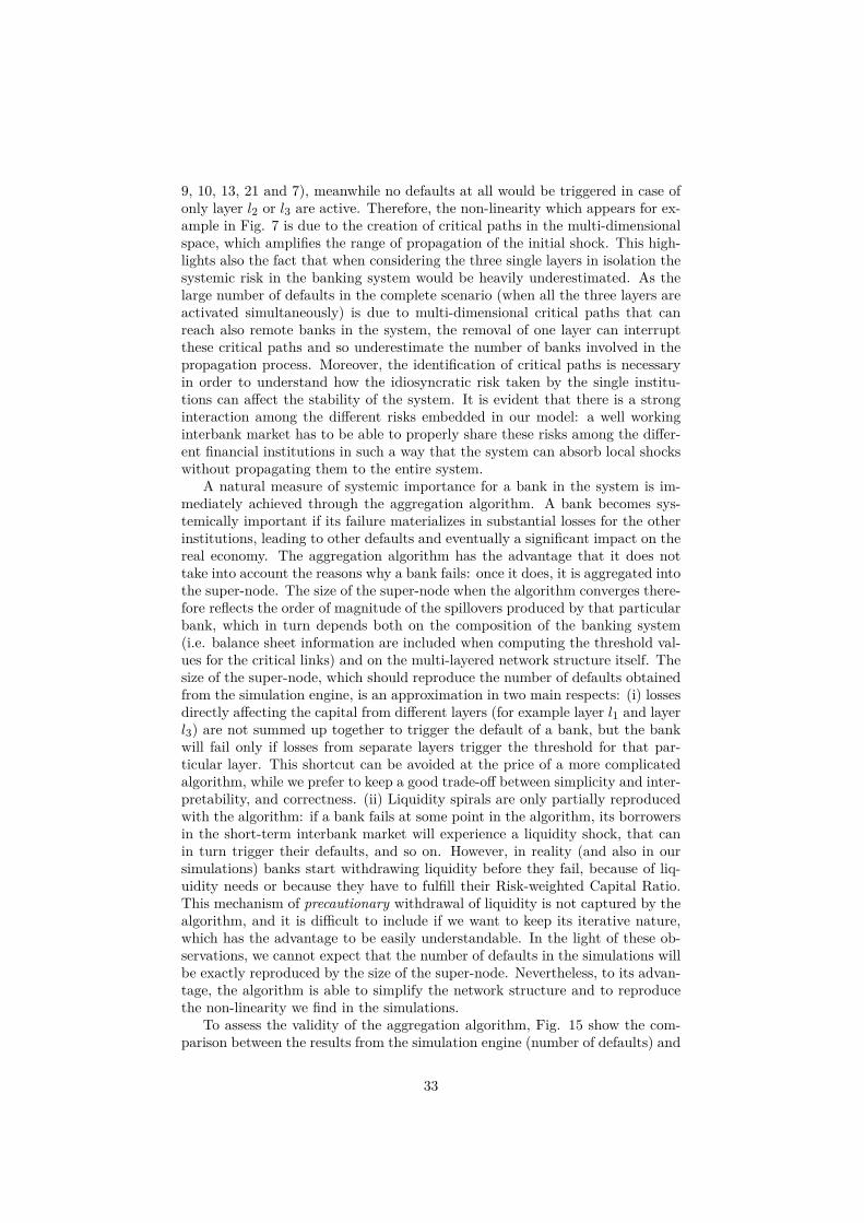
9, 10, 13, 21 and 7), meanwhile no defaults at all would be triggered in case ofonly layer l2 or l3 are active. Therefore, the non-linearity which appears for ex-ample in Fig. 7 is due to the creation of critical paths in the multi-dimensionalspace, which amplifies the range of propagation of the initial shock. This high-lights also the fact that when considering the three single layers in isolation thesystemic risk in the banking system would be heavily underestimated. As thelarge number of defaults in the complete scenario (when all the three layers areactivated simultaneously) is due to multi-dimensional critical paths that canreach also remote banks in the system, the removal of one layer can interruptthese critical paths and so underestimate the number of banks involved in thepropagation process. Moreover, the identification of critical paths is necessaryin order to understand how the idiosyncratic risk taken by the single institu-tions can affect the stability of the system. It is evident that there is a stronginteraction among the different risks embedded in our model: a well workinginterbank market has to be able to properly share these risks among the differ-ent financial institutions in such a way that the system can absorb local shockswithout propagating them to the entire system.

A natural measure of systemic importance for a bank in the system is im-mediately achieved through the aggregation algorithm. A bank becomes sys-temically important if its failure materializes in substantial losses for the otherinstitutions, leading to other defaults and eventually a significant impact on thereal economy. The aggregation algorithm has the advantage that it does nottake into account the reasons why a bank fails: once it does, it is aggregated intothe super-node. The size of the super-node when the algorithm converges there-fore reflects the order of magnitude of the spillovers produced by that particularbank, which in turn depends both on the composition of the banking system(i.e. balance sheet information are included when computing the threshold val-ues for the critical links) and on the multi-layered network structure itself. Thesize of the super-node, which should reproduce the number of defaults obtainedfrom the simulation engine, is an approximation in two main respects: (i) lossesdirectly affecting the capital from different layers (for example layer l1 and layerl3) are not summed up together to trigger the default of a bank, but the bankwill fail only if losses from separate layers trigger the threshold for that par-ticular layer. This shortcut can be avoided at the price of a more complicatedalgorithm, while we prefer to keep a good trade-off between simplicity and inter-pretability, and correctness. (ii) Liquidity spirals are only partially reproducedwith the algorithm: if a bank fails at some point in the algorithm, its borrowersin the short-term interbank market will experience a liquidity shock, that canin turn trigger their defaults, and so on. However, in reality (and also in oursimulations) banks start withdrawing liquidity before they fail, because of liq-uidity needs or because they have to fulfill their Risk-weighted Capital Ratio.This mechanism of precautionary withdrawal of liquidity is not captured by thealgorithm, and it is difficult to include if we want to keep its iterative nature,which has the advantage to be easily understandable. In the light of these ob-servations, we cannot expect that the number of defaults in the simulations willbe exactly reproduced by the size of the super-node. Nevertheless, to its advan-tage, the algorithm is able to simplify the network structure and to reproducethe non-linearity we find in the simulations.

To assess the validity of the aggregation algorithm, Fig. 15 show the com-parison between the results from the simulation engine (number of defaults) and

33

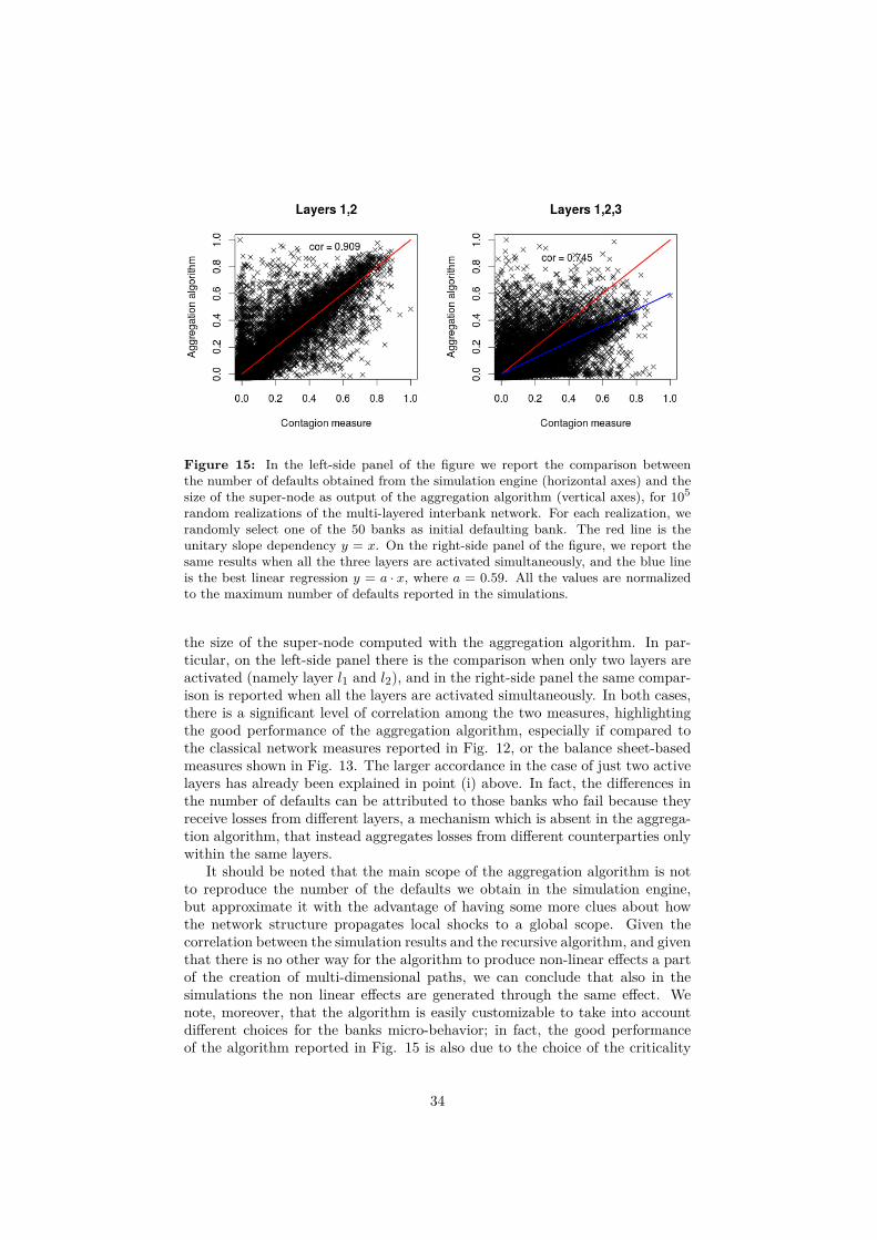
Figure 15: In the left-side panel of the figure we report the comparison betweenthe number of defaults obtained from the simulation engine (horizontal axes) and thesize of the super-node as output of the aggregation algorithm (vertical axes), for 105

random realizations of the multi-layered interbank network. For each realization, werandomly select one of the 50 banks as initial defaulting bank. The red line is theunitary slope dependency y = x. On the right-side panel of the figure, we report thesame results when all the three layers are activated simultaneously, and the blue lineis the best linear regression y = a · x, where a = 0.59. All the values are normalizedto the maximum number of defaults reported in the simulations.

the size of the super-node computed with the aggregation algorithm. In par-ticular, on the left-side panel there is the comparison when only two layers areactivated (namely layer l1 and l2), and in the right-side panel the same compar-ison is reported when all the layers are activated simultaneously. In both cases,there is a significant level of correlation among the two measures, highlightingthe good performance of the aggregation algorithm, especially if compared tothe classical network measures reported in Fig. 12, or the balance sheet-basedmeasures shown in Fig. 13. The larger accordance in the case of just two activelayers has already been explained in point (i) above. In fact, the differences inthe number of defaults can be attributed to those banks who fail because theyreceive losses from different layers, a mechanism which is absent in the aggrega-tion algorithm, that instead aggregates losses from different counterparties onlywithin the same layers.

It should be noted that the main scope of the aggregation algorithm is notto reproduce the number of the defaults we obtain in the simulation engine,but approximate it with the advantage of having some more clues about howthe network structure propagates local shocks to a global scope. Given thecorrelation between the simulation results and the recursive algorithm, and giventhat there is no other way for the algorithm to produce non-linear effects a partof the creation of multi-dimensional paths, we can conclude that also in thesimulations the non linear effects are generated through the same effect. Wenote, moreover, that the algorithm is easily customizable to take into accountdifferent choices for the banks micro-behavior; in fact, the good performanceof the algorithm reported in Fig. 15 is also due to the choice of the criticality

34

conditions appearing in eq.s (16)-(20), which reflect the micro behavior of banksin the system. Changing the banks micro-behavior, or including other, willreflect in different condition for the links criticality, but the algorithm can stillbe used to simplify the financial network structure.

7 Conclusions and policy implicationsThe agent-based, multi-layered interbank network model presented in this pa-per illustrates the importance of taking a holistic approach when analysing thecontagion risks related to the interconnections between banks. The main find-ing is that looking at segments of banks’ interconnections in isolation, withoutconsidering the interactions with other layers of banks’ interrelationships, canlead to a serious underestimation of interbank contagion risk. In other words, bytaking into account the various layers of interbank relations and the interactionsbetween them the contagion effects of a shock to one layer can be significantlyamplified, compared to the situation where contagion risks are assumed to beconfined within the specific layer where the initial shock arose. This findingpoints to the existence of important non-linearities in the way bank-specificshocks are propagated throughout the financial system.

Another important finding of the paper is that the structure of the networkand the underlying balance sheet positions of the banks (nodes) in the networkmatter in terms of resilience to shocks. In many, in fact the majority, of oursimulated network structures financial contagion is likely to be limited. However,in certain network constellations, also depending on the financial soundnessof the central players in those networks, contagion risk is substantially morepronounced.

Furthermore, by considering not only contagion via direct bilateral expo-sures but also via banks’ common exposures (through their securities holdings)we are able to demonstrate a trade-off between risk diversification decisions andfinancial stability. In other words, due to the potential contagion risks relatedto banks’ common exposures decisions to diversify their investments in securi-ties that may be optimal at the individual bank level can in fact imply highercontagion risks for the system as a whole.

In view of these findings, the paper proposes a “systemic importance” mea-sure that accounts for the multi-dimensional aspect of banks’ interrelations.That is, based on our multi-layered network model and taking into account in-dividual banks’ balance sheet structure the approach provides a single measureof banks’ systemic importance that outperforms standard network centralitymeasures as well as typical balance sheet indicators.

The observation that unless a holistic view of banks’ interrelations is takenthe analysis of interbank contagion risk is likely to underestimate the true con-tagion risk has major policy implications. From both a micro-prudential andin particular a macro-prudential perspective the findings of this paper suggestthat it is insufficient to analyse contagion within specific market segments inisolation. Indeed, according to the findings presented here, a major componentof the propagation mechanism that transmits losses in one bank to the rest ofthe system derives from the interactions between the multiple layers of inter-actions that banks have with each other. On this basis, an immediate policyprescription emerging from this analysis is the importance of collecting adequate

35

supervisory data that allows for assessing in a holistic way the interconnected-ness of the banking system and thus account for the non-linearities that theexistence of multi-layered interbank networks may induce.

References[1] Allen, F. and Gale, D., ’Financial contagion’, Journal of Political

Economy, Vol. 108, pages 1-33, 2000

[2] Battiston, S., Puliga, M., Kaushik, R., Tasca, P., Caldarelli, G.,’DebtRank: Too Central to Fail? Financial Networks, the FEDand Systemic Risk’, Scientific Reports 2, Article number 541, 2012

[3] Beale, N., Rand, D. G., Battey, H., Croxson, K., May, R. M.,Nowark, M. A., ’Individual versus systemic risk and the Regulator’sDilemma’, PNAS 2011 108(31), 2011

[4] Bluhm, M. and Krahnen, J. P. ’Default Risk in an interconnectedBanking System with Endogenous Asset Markets’, CFS WorkingPaper Series No. 2011/19

[5] Bisias, D., Flood, M. D., Lo, A. W., Valavanis, S., ’A Survey ofSystemic Risk Analytics’, U.S. Department of Treasury, Office ofFinancial Research No. 0001, 2012

[6] Brunnermeier, M. K., ’Deciphering the Liquidity and CreditCrunch 2007-2008’, Journal of Economic Perspectives, Volume 23,Number 1, p. 77-100, 2009

[7] Diamond, D. W. and Dybvig P. H., ’Bank Runs, Deposit Insurance,and Liquidity’, The Journal of Political Economy, Vol. 91, No. 3,pp. 401-419, 1983

[8] Delpini, D., Battiston, S., Riccaboni, M., Gabbi, G., Pammolli, F.,Caldarelli, G. ’Evolution of Controllability in Interbank Networks’,Scientific Reports 3, Article number 1626, 2013

[9] Eisenberg, L., Noe, T. H., ’Systemic Risk in Financial System’,Management Science, vol. 47 no. 2 236’249, 2001

[10] Gai, P. and S. Kapadia, ’Contagion in Financial Networks’, Work-ing paper no 383/2010, Bank of England, 2010

[11] Georg, C. ’The effect of the interbank network structure on conta-gion and common shocks’, DeutscheBank Discussion Paper, Series2: Banking and Financial Studies No 12/2011

[12] Gómez, S., Diaz-Guilera, A., Gómez-Gardeñes, J., Pérez-Vicente,C.J., Moreno, Y., Arenas, A. ’Diffusion dynamics on multiplexnetworks’, arXiv:1207.2788 [physics.soc-ph]

[13] Halaj, G. and Kok, C. S., ’Assessing Interbank Contagion UsingSimulated Networks’, ECB Working Paper No. 1506, 2013

36

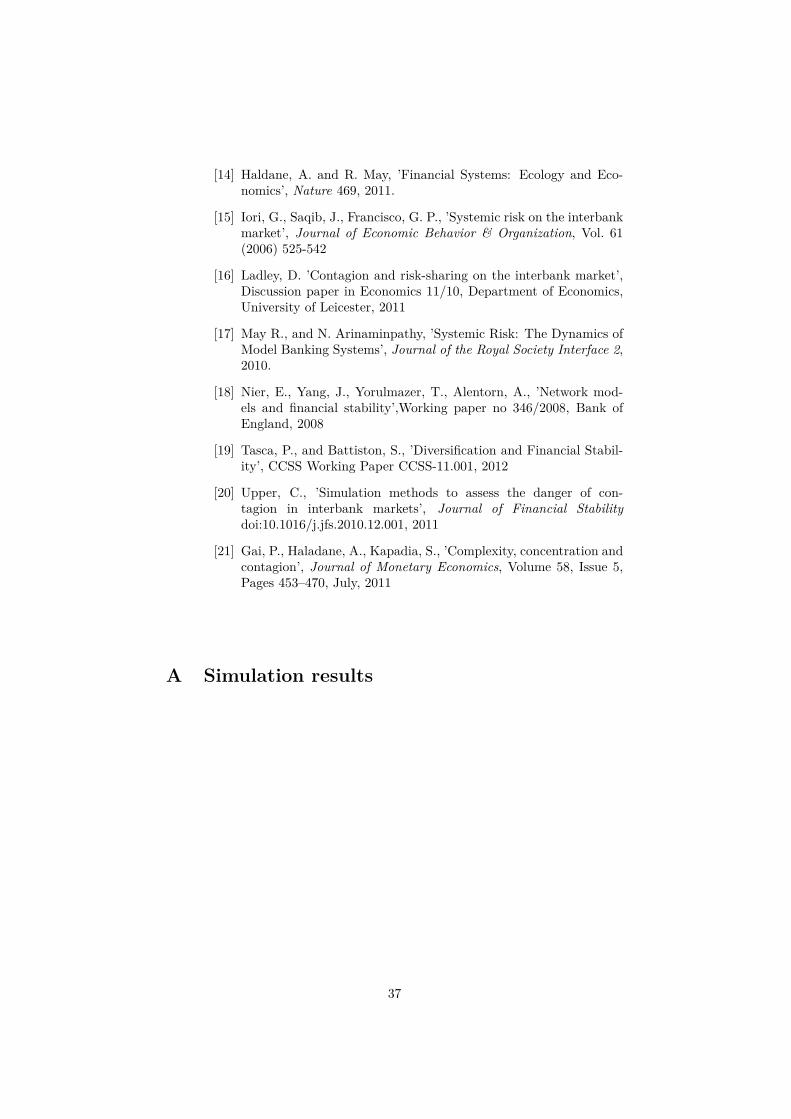
[14] Haldane, A. and R. May, ’Financial Systems: Ecology and Eco-nomics’, Nature 469, 2011.

[15] Iori, G., Saqib, J., Francisco, G. P., ’Systemic risk on the interbankmarket’, Journal of Economic Behavior & Organization, Vol. 61(2006) 525-542

[16] Ladley, D. ’Contagion and risk-sharing on the interbank market’,Discussion paper in Economics 11/10, Department of Economics,University of Leicester, 2011

[17] May R., and N. Arinaminpathy, ’Systemic Risk: The Dynamics ofModel Banking Systems’, Journal of the Royal Society Interface 2,2010.

[18] Nier, E., Yang, J., Yorulmazer, T., Alentorn, A., ’Network mod-els and financial stability’,Working paper no 346/2008, Bank ofEngland, 2008

[19] Tasca, P., and Battiston, S., ’Diversification and Financial Stabil-ity’, CCSS Working Paper CCSS-11.001, 2012

[20] Upper, C., ’Simulation methods to assess the danger of con-tagion in interbank markets’, Journal of Financial Stabilitydoi:10.1016/j.jfs.2010.12.001, 2011

[21] Gai, P., Haladane, A., Kapadia, S., ’Complexity, concentration andcontagion’, Journal of Monetary Economics, Volume 58, Issue 5,Pages 453–470, July, 2011

A Simulation results

37

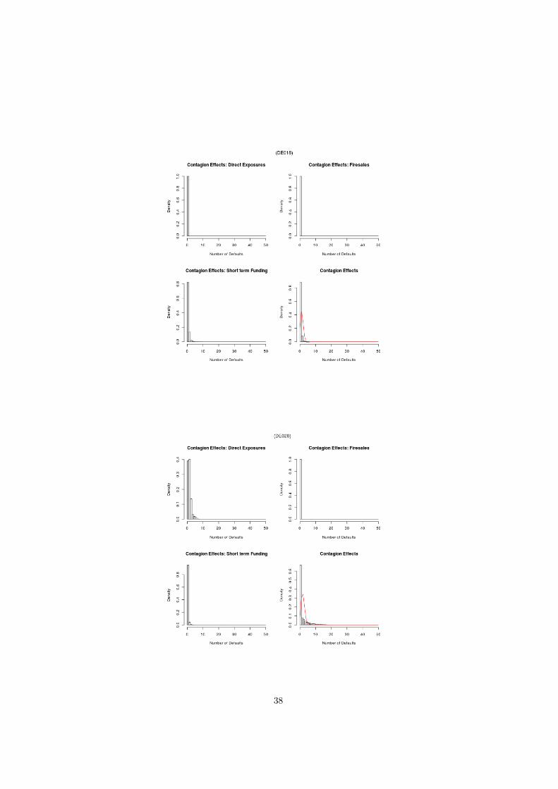
38

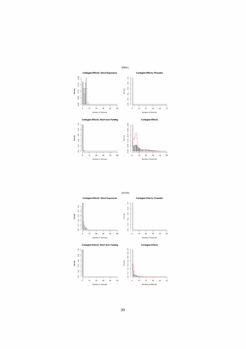
39

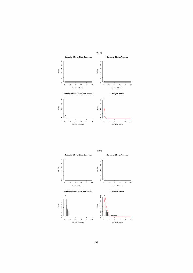
40

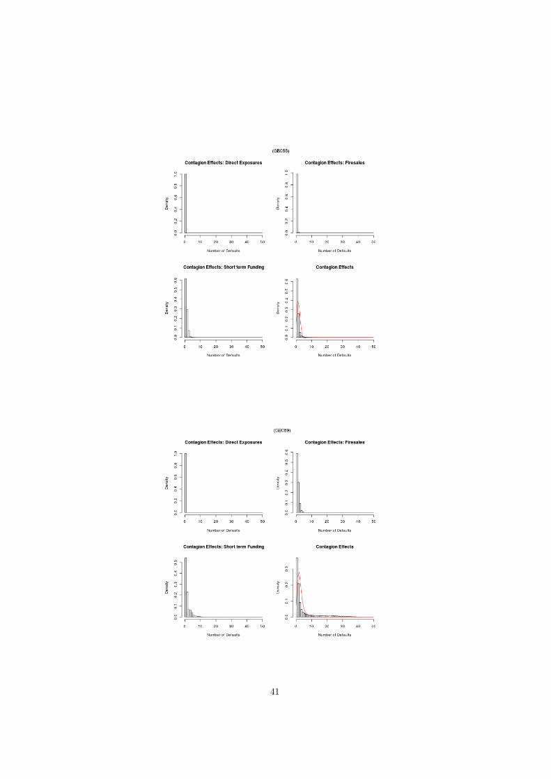
41

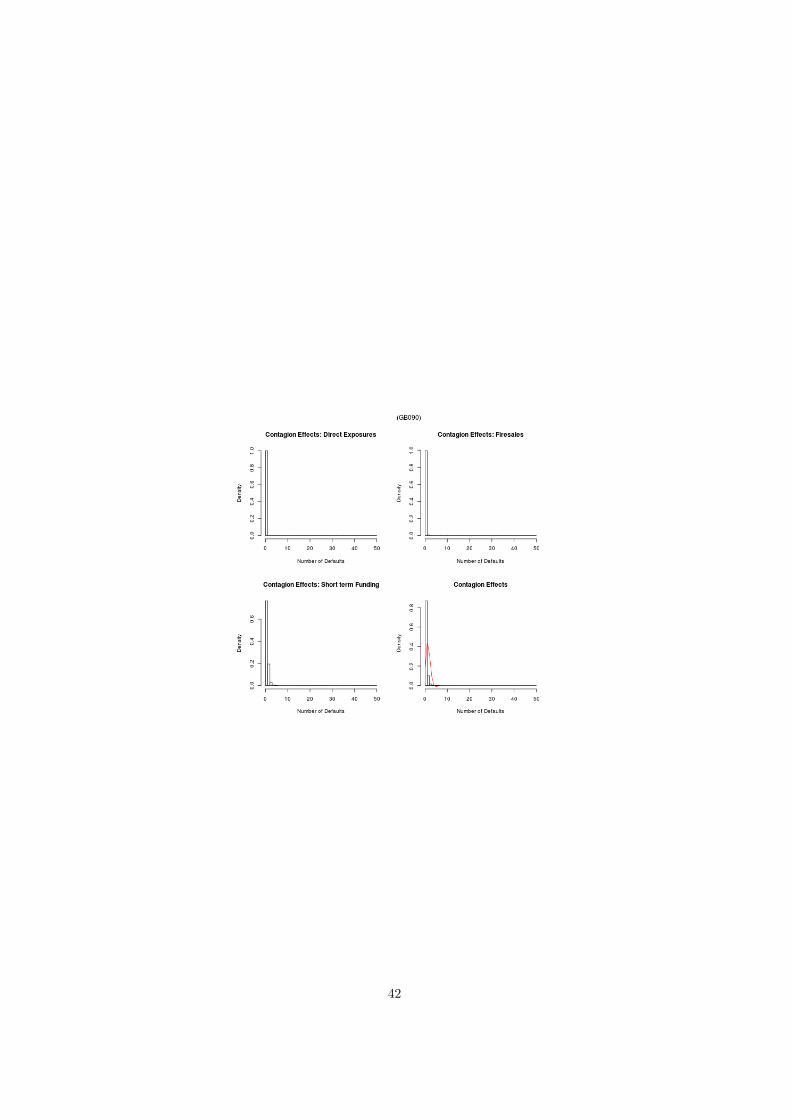
42