Multi Instance Anomaly Detection in BusinessProcess Executions

Kristof Bohmer and Stefanie Rinderle-Ma

University of Vienna, Faculty of Computer Science{kristof.boehmer,stefanie.rinderle-ma}@univie.ac.at

Abstract. Processes control critical IT systems and business cases indynamic environments. Hence, ensuring secure model executions is cru-cial to prevent misuse and attacks. In general, anomaly detection ap-proaches can be employed to tackle this challenge. Existing ones analyzeeach process instance individually. Doing so does not consider attacksthat combine multiple instances, e.g., by splitting fraudulent fund trans-actions into multiple instances with smaller “unsuspicious” amounts. Theproposed approach aims at detecting such attacks. For this, anomaliesbetween the temporal behavior of a set of historic instances (ex post) andthe temporal behavior of running instances are identified. Here, tempo-ral behavior refers to the temporal order between the instances and theirevents. The proposed approach is implemented and evaluated based onreal life process logs from different domains and artificial anomalies.

Keywords: Runtime Anomaly Detection, Secure Business Processes,Multiple Instances, Temporal Anomalies

1 Introduction

Business process anomaly detection identifies anomalous behavior in recorded(ex post) or ongoing (real time) process executions in order to expose and preventfraud, misuse, unknown attacks, and errors. Hence it constitutes a critical ITsecurity defense line in today’s interconnected business driven organizations [3,5]. Existing process anomaly detection work analyzes single process instances inorder to distinguish if their behavior is anomalous (i.e., unlikely) or not. Doingso does not provide protection against all possible attack vectors. For example,assume an attack scenario where the attacker (Trudy) strives to quickly transferfunds from an organization’s bank account. Therefore, Trudy could instantiatea single transaction process and transfer all the money at once. Alternatively,Trudy could start multiple transaction processes in parallel and split up thetransactions into smaller chunks. The first approach would likely be detected byexisting anomaly detection approaches while the second would not.

This is, because in the first case the transferred funds are exceptionally high,i.e., they exceed previously transferred funds and are, therefore, unlikely. Inthis case, analyzing each process instance execution individually is sufficient toidentify Trudy’s attack. In the second case each individual process instance only

transfers a small amount of money. Through this, the transferred funds are,likely, comparable to transactions represented in the known historic behavior.Accordingly the executions would not be identified as anomalous.

Hence, an anomaly detection approach is required that is able to considermultiple instances – from the same or different process models. In the examplescenario these are instances which take place before, during, or after one of thefraudulent transaction process executions. Through this the parallel executionsare noticed as unusual and the second attack scenario is identified. The assump-tion behind this is that the massive parallel execution of multiple transactionprocesses – which was never observed before – is unlikely (i.e., anomalous).

This paper proposes a configurable and unsupervised anomaly detectionheuristic for business processes that exploits the temporal dependencies betweenmultiple instances. In detail, for each instance of interest, all temporal relationsof preceding, succeeding, and simultaneous process executions are taken intoaccount. The business process instances and executions which are taken intoconsideration can stem from various models, i.e., not all instances need to bespawned from the same process model but, e.g., from multiple models.

This work applies design science research, cf. [14]. Doing so multi instanceprocess executions were identified as a problem (i.e., an unprotected attack vec-tor). To tackle this problem artifacts are created and evaluated, here this is aprototypical implementation of the proposed multi instance anomaly detectionapproach. Stakeholders for the approach are organizations and security experts.

More precisely, we assume a set of process models R, and a set of executionlog files L. Hereby, R could be a process repository and L holds all executions ofthe processes in R. The key idea is to generate an anomaly detection signatureG for a process P ∈ R so that it represents for P the behavior of P ’s instancesand temporally related instances from multiple other models. This is achievedby mining and combining temporal relations from multiple instances, stored inL, that take place during or close to executions of P into a signature G.

Finally, behavior that should be analyzed for anomalies, from P ’s instancesand other temporally related instances, is assumed as given. For example, suchbehavior can be extracted from logs, for ex post analysis, or be collected directlyduring model executions – from process execution engines – for real time analysis.To analyze if behavior is anomalous or not it is mapped to G, which enables tocalculate its behavior likelihood. If the behavior to analyze for anomalies is foundto be unlikely, when comparing it to the logged historic behavior in L, then thebehavior is identified as anomalous. The artifacts generated in this work comprisemulti instance process behavior mining and signature generation and matchingalgorithms. The presented approach is evaluated using real life process executionlogs from multiple domains along with artificially generated anomalies.

This paper is organized as follows: Related work is discussed in Section 2.Prerequisites and the proposed approach are introduced in Section 3. The pro-posed anomaly detection approach (i.e., signature generation and matching) is,in detail, described in Section 4. Section 5 holds the evaluation. Finally, conclu-sions, discussions, and future work is given in Section 6.

2 Related Work

Related anomaly detection work was searched for in the process domain andin the security domain. The results found for the process domain were limitedas related work focuses only on single individual process models and instances.Hence, the anomalies which this work is capable of identifying are not supportedby existing process anomaly detection work. Our systematic literature review in[6] provides a more detailed analysis. The most comparable work [12] analyzestemporal behavior of individual activities to identify unlikely anomalous execu-tion behavior. However, this work also concentrates only on single instances.

In a broader context, i.e., the security domain in general, several temporalanomaly detection approaches are suggested, cf. [10]. However, according to [10]and our own findings, those approaches are typically domain or data specific (i.e.,focus on specific protocols, such as, SIP or network packages) and can, because ofthis, hardly be generalized, e.g., to analyze process behavior data for anomalies.It can be concluded that an anomaly detection approach specifically tailored forprocess behavior is a necessity to identify related attacks and anomalies.

Moreover, it was found that existing approaches show, likely, an underwhelm-ing anomaly detection performance when dealing with unexpected behavior. Ex-isting anomaly detection work frequently classifies unexpected behavior, even ifit only slightly deviates from, e.g., a signature, as anomalous. This could po-tentially result in a large amount of false positives [5] in flexible and dynamicexecution scenarios. Hence, this work proposes a novel approach to deal withunexpected behavior by assigning it with an artificially calculated likelihood.

Existing approaches which are comparable to the presented artificial likeli-hood calculation are so called soft matching techniques. Soft matching general-izes expected behavior patterns by constructing multiple slightly deviating, butstill presumably “correct” patterns (e.g., based on expert knowledge) [2]. Herebythe area of data or behavior which is identified as non-anomalous is widened.Unfortunately, it frequently requires expert knowledge to soften the patternsand through this soft matching lacks in flexibility, compared to the presentedautomatic approach. Moreover, the presented approach enables to “aggregate”multiple occurrences of slightly unlikely behavior to identify collective anoma-lies [5] which could be missed by less sensitive detection approaches. This isbecause this work does not flag each observed process execution behavior solelyas anomalous or non-anomalous. Instead a more flexible likelihood is calculatedand aggregated over multiple successive process execution events and instances.

3 Prerequisites and General Approach

This paper proposes a multi instance anomaly detection approach that enablesto distinguish process execution behavior as anomalous (i.e., unlikely) or not.For this the behavior is compared with a signature generated from given processexecution logs L which represent historic process executions. Generating signa-tures from logs is beneficiary as logs are frequently generated automatically by

today’s process execution engines, contain real behavior and executions, and in-clude manual adaptations. Moreover, exploiting execution logs enables to becomeindependent from abstracted and potentially outdated documentation [11].

Let each execution log l ∈ L hold the associated process model name anda bag of execution Events, i.e., l := (n,E). Each execution event e ∈ l.E, i.e.,e := (s, c) represents an activity execution by its start and completion timestamps and c respectively, with s, c ∈ N>0. An exemplary log for model A with twoactivity executions could be defined as lA := (A, {(s1, c1), (s2, c2)}). We assumethat each individual model execution (i.e., each instance) is held by an individualexecution log l ∈ L and that timestamps are defined in a range of N>0.

Such a brief definition is sufficient because the presented approach mainlyanalyzes temporal relations between models and their instances. For this thefollowing auxiliary functions, inspired by a subset of Allen’s interval algebra [1],are defined. The start timestamp of an instance execution is found by min(E) :={e.s|e ∈ E;∀e′ ∈ E, e.s ≤ e′.s}0. Here, {· · · }0 returns the only element heldby a set or bag if it is a singleton or a random set/bag element if it is not.A similar definition is applied for max(E) to determined the end timestamp ofan instance execution. Through this the duration of an instance is dur(E) :=max(E)− min(E). Moreover, execP(t, L) extracts a bag of process model namesthat are executed at point t (i.e., a timestamp) based on the logs in L, i.e.,execP(t, L) := {l.n|∃l ∈ L,∃e ∈ l.E; e.s ≤ t ∧ e.c ≥ t}. Similarly, act(t1, t2, L)counts the activities that are executed in a specific interval given by t1, t2, i.e.,act(t1, t2, L) := |{e|l ∈ L, e ∈ l.E; e.s ≥ t1 ∧ e.c ≤ t2}| where t1 ≤ t2. Functionnext(t, L) determines the process instance start or end timestamp that occurs asclose after t as possible, i.e., next(t, L) := {t1|t1, t2 ∈ T ;@t2 < t1; t1 > t∧t2 > t}0where T := {e.s|l ∈ L, e ∈ l.E} ∪ {e.c|l ∈ L, e ∈ l.E}. Further, mid(t1, t2) :=t1 + ((t2 − t1)/2) calculates the average of two timestamps where t1 < t2.

Fig. 1. Proposed multi instance anomaly detection approach – overview

Fig. 1 provides an overview on the proposed anomaly detection heuristic.The related algorithms are presented in Sect. 4. Firstly, a signature is generatedfor a process P ∈ R based on a set L of historic instance executions – both areassumed as given input. The first idea is to extract process execution events inL that precede, succeed, or occur simultaneously to executions of P ’s instances,cf. Fig. 2. The figure depicts three processes – A, B, and C – along with anumber of instances (i.e., the rectangles, e.g., AI1 to AI4) and activity executionevents (i.e., the vertical bars in the instance rectangles, e.g., AI3 holds 4 activityexecutions). For the sake of brevity Fig. 2 depicts only a snapshot of all instanceexecutions, i.e., additional instances are stored in L but not depicted.

Assume a signature is generated for process B in Fig. 2. Then the signaturegeneration starts by identifying relevant execution events in L (i.e., historic

Fig. 2. Running example for window & behavior extraction and noise reduction

behavior) 1 . Relevant events are events which most likely affect B’s instances(i.e., events which precede B’s instances) or which are affected by B’s instances(i.e., events which are succeeding and simultaneous to B’s instances). Extractionwindows are applied to identify such events in the following.

An individual extraction window w := [wt1;wt2] is created for each of B’sinstances 1 . Extraction windows enable to determine which of the behaviorheld by L is relevant (i.e., preceding, succeeding, and simultaneous events) for aspecific instance and model and should, therefore, be contained in the generatedsignature. The beginning and end of the window (i.e., wt1 and wt2) is calculatedby multiplying the duration of the respective instance (this example uses BI3and lBI3 ∈ L) with a user chosen window size modifier ws ∈ R>0. So wt1 :=min(l.E) − (ws · dur(l.E)) and wt2 := max(l.E) + (ws · dur(l.E)). Hence, whenassuming ws = 2 and min(lBI3.E) = ts9, max(lBI3.E) = ts13 then wBI3 = [ts1; ts21].

The size of an extraction window is defined in a direct relation to the durationof the corresponding instance. Moreover, the parameter ws enables to adapt theextraction window size to the density of the analyzed event logs. For example,if a log is very dense (i.e., it holds a large amount of events in a short timespan)then applying extraction windows with a fixed size could result in an overlydetailed signature (i.e., overfitting occurs) which could, subsequently, lead toflawed anomaly detection results, cf. [7]. In comparison a sparse log combinedwith a fixed size window could result in a signature that contains insufficienthistoric behavior to identify anomalies (i.e., underfitting occurs).

Subsequently step 2 is applied to mine all the behavior that occurs in achosen window in a time sequence. Therefore, the window is split into multipleslots based on the start and end of the process instances covered by the window(i.e, the dotted lines and slot timestamps in Fig. 2). Each slot is defined aso := (N, tss, t

se) where tss and tse represent the start and end timestamps of the

slot and the bag N := execP(mid(tss, tse), L) holds the names of models whose

instances occur between tss and tse. For example, slot 5 in Fig. 2 would be definedas o5 = ({A,B,C}, ts5, ts6). If multiple instances from the same process modelare executed in parallel then the related model’s name occurs in o.N multipletimes (e.g., two parallel executions of model A would result in o.N = {A,A}).Subsequently, all slots are combined into a time sequence, i.e., an ordered listof slots ts := 〈o1, o2, · · · , on〉, e.g., tsBI3 = 〈o1, o2, · · · , o20〉 for instance BI3, cf.

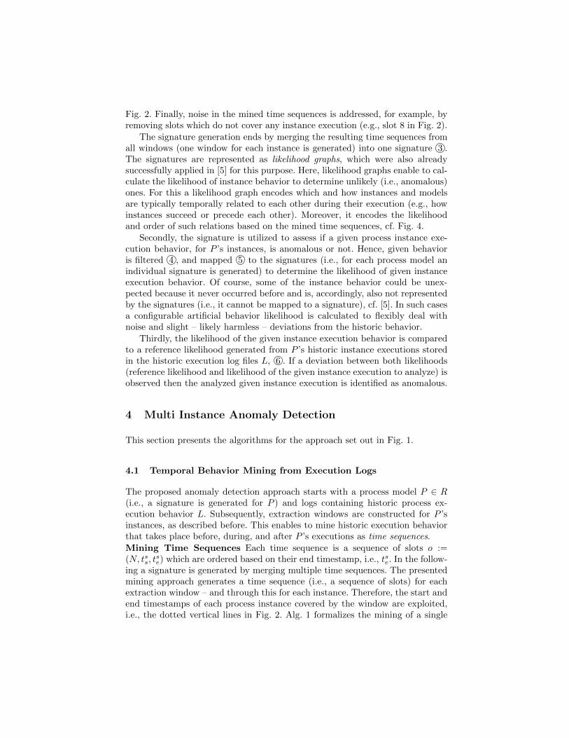
Fig. 2. Finally, noise in the mined time sequences is addressed, for example, byremoving slots which do not cover any instance execution (e.g., slot 8 in Fig. 2).

The signature generation ends by merging the resulting time sequences fromall windows (one window for each instance is generated) into one signature 3 .The signatures are represented as likelihood graphs, which were also alreadysuccessfully applied in [5] for this purpose. Here, likelihood graphs enable to cal-culate the likelihood of instance behavior to determine unlikely (i.e., anomalous)ones. For this a likelihood graph encodes which and how instances and modelsare typically temporally related to each other during their execution (e.g., howinstances succeed or precede each other). Moreover, it encodes the likelihoodand order of such relations based on the mined time sequences, cf. Fig. 4.

Secondly, the signature is utilized to assess if a given process instance exe-cution behavior, for P ’s instances, is anomalous or not. Hence, given behavioris filtered 4 , and mapped 5 to the signatures (i.e., for each process model anindividual signature is generated) to determine the likelihood of given instanceexecution behavior. Of course, some of the instance behavior could be unex-pected because it never occurred before and is, accordingly, also not representedby the signatures (i.e., it cannot be mapped to a signature), cf. [5]. In such casesa configurable artificial behavior likelihood is calculated to flexibly deal withnoise and slight – likely harmless – deviations from the historic behavior.

Thirdly, the likelihood of the given instance execution behavior is comparedto a reference likelihood generated from P ’s historic instance executions storedin the historic execution log files L, 6 . If a deviation between both likelihoods(reference likelihood and likelihood of the given instance execution to analyze) isobserved then the analyzed given instance execution is identified as anomalous.

4 Multi Instance Anomaly Detection

This section presents the algorithms for the approach set out in Fig. 1.

4.1 Temporal Behavior Mining from Execution Logs

The proposed anomaly detection approach starts with a process model P ∈ R(i.e., a signature is generated for P ) and logs containing historic process ex-ecution behavior L. Subsequently, extraction windows are constructed for P ’sinstances, as described before. This enables to mine historic execution behaviorthat takes place before, during, and after P ’s executions as time sequences.

Mining Time Sequences Each time sequence is a sequence of slots o :=(N, tss, t

se) which are ordered based on their end timestamp, i.e., tse. In the follow-

ing a signature is generated by merging multiple time sequences. The presentedmining approach generates a time sequence (i.e., a sequence of slots) for eachextraction window – and through this for each instance. Therefore, the start andend timestamps of each process instance covered by the window are exploited,i.e., the dotted vertical lines in Fig. 2. Alg. 1 formalizes the mining of a single

Algorithm mineTS(extraction window w := [wt1;wt2], execution logs L)Result: mined time sequence tsts := 〈〉; first := w.wt1 // initially ts is empty// extract the interval between instance start and end timestamps as slotswhile second := next(first, L) ∧ second < w.wt2 do

ts := ts⊕ (execP(mid(first, second), L), first, second)first := second // preserve for next iteration

// interval from the last instance start or end till the end of the windowts := ts⊕ (execP(mid(first, w.wt2), L), first, w.wt2))return ts // the mined time sequence for the window w and a given log L

Algorithm 1: Mines a time sequence for a given window w and logs L

time sequence for a given window w and the historic execution logs in L. In thefollowing the symbol ⊕ denotes the appending of a slot to the end of a sequence.

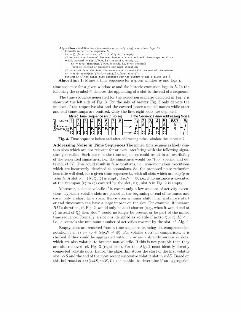
The time sequence generated for the execution scenario depicted in Fig. 2 isshown at the left side of Fig. 3. For the sake of brevity Fig. 3 only depicts thenumber of the respective slot and the covered process model names while startand end timestamps are omitted. Only the first eight slots are depicted.

Fig. 3. Time sequence before and after addressing noise, window size is ws = 2

Addressing Noise in Time Sequences The mined time sequences likely con-tain slots which are not relevant for or even interfering with the following signa-ture generation. Such noise in the time sequences could result in an overfittingof the generated signatures, i.e., the signatures would be “too” specific and de-tailed, cf. [7]. This could result in false positives, i.e., non-anomalous executionswhich are incorrectly identified as anomalous. So, the proposed noise reductionheuristic will deal, for a given time sequence ts, with all slots which are empty orvolatile. A slot o := (N, tss, t

se) is empty if o.N = ∅, i.e., if no instance is executed

at the timespan (tss to tse) covered by the slot, e.g., slot 8 in Fig. 2 is empty.

Moreover, a slot is volatile if it covers only a low amount of activity execu-tions. Typically volatile slots are placed at the beginning or end of instances andcover only a short time span. Hence even a minor shift in an instance’s startor end timestamp can have a large impact on the slot. For example, if instanceBI2’s duration, cf. Fig. 2, would only be a bit shorter (e.g., when it would end atts7 instead of ts8) then slot 7 would no longer be present or be part of the minedtime sequence. Formally, a slot o is identified as volatile if act(o.tss, o.t

se, L) < c,

i.e., c controls the minimum number of activities covered by the slot, cf. Alg. 2.

Empty slots are removed from a time sequence ts, using list comprehensionnotation, i.e., ts := 〈o ∈ ts|o.N 6= ∅〉. For volatile slots, in comparison, it ischecked if they could be aggregated with one or more directly successive slots,which are also volatile, to become non-volatile. If this is not possible then theyare also removed, cf. Fig. 3 (right side). For this Alg. 2 must identify directlyconnected volatile slots. Hence, the algorithm stores the start of the first volatileslot volS and the end of the most recent successive volatile slot in volE. Based onthis information act(volS, volE, L) > c enables to determine if an aggregation

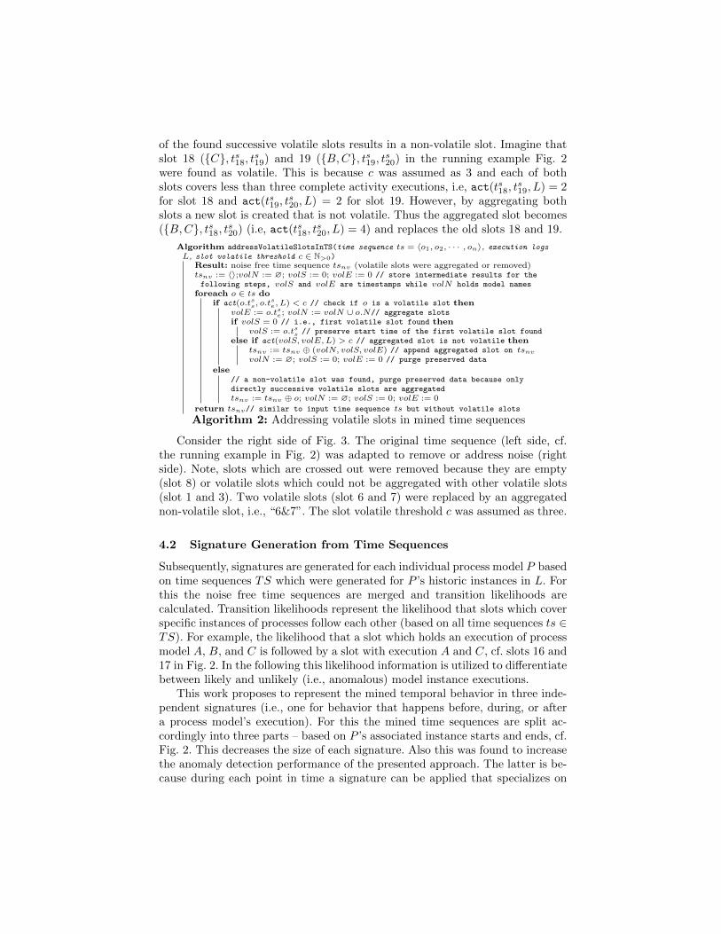
of the found successive volatile slots results in a non-volatile slot. Imagine thatslot 18 ({C}, ts18, ts19) and 19 ({B,C}, ts19, ts20) in the running example Fig. 2were found as volatile. This is because c was assumed as 3 and each of bothslots covers less than three complete activity executions, i.e, act(ts18, t

s19, L) = 2

for slot 18 and act(ts19, ts20, L) = 2 for slot 19. However, by aggregating both

slots a new slot is created that is not volatile. Thus the aggregated slot becomes({B,C}, ts18, ts20) (i.e, act(ts18, t

s20, L) = 4) and replaces the old slots 18 and 19.

Algorithm addressVolatileSlotsInTS(time sequence ts = 〈o1, o2, · · · , on〉, execution logsL, slot volatile threshold c ∈ N>0)

Result: noise free time sequence tsnv (volatile slots were aggregated or removed)tsnv := 〈〉;volN := ∅; volS := 0; volE := 0 // store intermediate results for thefollowing steps, volS and volE are timestamps while volN holds model names

foreach o ∈ ts doif act(o.tss, o.t

se, L) < c // check if o is a volatile slot then

volE := o.tse; volN := volN ∪ o.N// aggregate slotsif volS = 0 // i.e., first volatile slot found then

volS := o.tss // preserve start time of the first volatile slot foundelse if act(volS, volE, L) > c // aggregated slot is not volatile then

tsnv := tsnv ⊕ (volN, volS, volE) // append aggregated slot on tsnv

volN := ∅; volS := 0; volE := 0 // purge preserved data

else// a non-volatile slot was found, purge preserved data because onlydirectly successive volatile slots are aggregatedtsnv := tsnv ⊕ o; volN := ∅; volS := 0; volE := 0

return tsnv// similar to input time sequence ts but without volatile slots

Algorithm 2: Addressing volatile slots in mined time sequences

Consider the right side of Fig. 3. The original time sequence (left side, cf.the running example in Fig. 2) was adapted to remove or address noise (rightside). Note, slots which are crossed out were removed because they are empty(slot 8) or volatile slots which could not be aggregated with other volatile slots(slot 1 and 3). Two volatile slots (slot 6 and 7) were replaced by an aggregatednon-volatile slot, i.e., “6&7”. The slot volatile threshold c was assumed as three.

4.2 Signature Generation from Time Sequences

Subsequently, signatures are generated for each individual process model P basedon time sequences TS which were generated for P ’s historic instances in L. Forthis the noise free time sequences are merged and transition likelihoods arecalculated. Transition likelihoods represent the likelihood that slots which coverspecific instances of processes follow each other (based on all time sequences ts ∈TS). For example, the likelihood that a slot which holds an execution of processmodel A, B, and C is followed by a slot with execution A and C, cf. slots 16 and17 in Fig. 2. In the following this likelihood information is utilized to differentiatebetween likely and unlikely (i.e., anomalous) model instance executions.

This work proposes to represent the mined temporal behavior in three inde-pendent signatures (i.e., one for behavior that happens before, during, or aftera process model’s execution). For this the mined time sequences are split ac-cordingly into three parts – based on P ’s associated instance starts and ends, cf.Fig. 2. This decreases the size of each signature. Also this was found to increasethe anomaly detection performance of the presented approach. The latter is be-cause during each point in time a signature can be applied that specializes on

the specific kind of behavior that is currently observed (e.g., behavior that washistorically observed after or during an instance execution). Hereby, the appliedsignature can be more specific than one large generic signature that needs tocover all the historic instance behavior (i.e., before, during, and after) at once.

Each signature is represented as a likelihood graph G = (V,D), cf. [5]. Alikelihood graph is a directed cyclic graph that consists of a set of vertexesv ∈ V and a set of edges d ∈ D with D ⊆ V × V × [0; 1]. Each vertex vrepresents processes covered by a specific o.N for a given slot o. In comparisoneach edge d = (vs, ve, tl) represents the transition likelihood tl ∈ [0; 1] from one“slot” vs (i.e., a vertex holding the process model names covered by a slot) toanother vertex ve based on the mined time sequences ts ∈ TS.

Alg. 3 creates a likelihood graph (i.e., a signature) by merging multiple timesequences. For this, the algorithm extracts from each slot, covered by the mergedtime sequences, the processes covered by that slot and stores them in the set V .Moreover, the set V C is populated with triplets vc = (v1, v2, tc) that indicate,based on the analyzed time sequences, that a slot v2 is preceded by a slot v1, tc ∈N>0 times (i.e., tc denotes the transition count). Subsequently these absolutenumbers (i.e., tc) are converted into relative transition likelihoods tl and storedinto D as edges. V is initialized with a dummy entry vd that is used as a generalentry point for the signature and the following mapping of behavior to it.

Algorithm mergeTimeSequencesIntoSignature(time sequences TS, dummy vertex, i.e., theentry point for the signature vd)

Result: likelihood graph (i.e., a signature) G = (V,D) from the behavior in TSV := {vd}; D := ∅; V C := ∅foreach ts ∈ TS where |ts| > 0 do

V C := V C ∪ {(vd, ts0, 1)} // add dummy vertex, ts0 identifies the first slot ints, i.e., tsi with 0 ≥ i < |ts| identifies the slot with the index i

for i := 0;i < (|ts| − 1);i := i+ 1 dov1 := tsi.N ; v2 := tsi+1.N// tsi and its successor tsi+1 in tsV := V ∪ {v1, v2};// add slots to signature graph vertex set Vtcount := 1// holds how frequently v1 is followed by v2 in all sequencesif (v1, v2, ·) ∈ V C // previous ts contained the same transition then

tcount := tcount+ {vc.tc|vc ∈ V C, vc.v1 = v1 ∧ vc.v2 = v2}0// purge old information for v1/v2, then add updated or new informationV C := {vc ∈ V C|vc.v1 6= v1 ∧ vc.v2 6= v2} ∪ {(v1, v2, tcount)}

foreach vc ∈ V C // convert absolute numbers into likelihoods dos := vc.tc;TC := {vc′.tc|vc′ ∈ V C ∧ vc′.v1 = vc.v1}// create and add edges to D that connect the signature vertexes in VD := D ∪ {(vc.v1, vc.v2, s∑

tcs∈TC tcs)}// fraction 7→ transaction likelihood

return G = (V,D)// return signature, it was created for sequences in TS

Algorithm 3: Merge time sequences TS for P into a signature G

Fig. 4 depicts an example for the proposed signature generation. Two timesequences (XI1 and XI2, mined for the process “X” – left side) are mergedinto a likelihood graph signature representation (right side). The depicted timesequences and represented behavior occurred after X’s instances (i.e., succeedingbehavior). So processX is placed at the start of the time sequences and signature.

4.3 Signature Matching for Execution Event Streams and Logs

The signatures are applied to calculate the likelihood of process execution be-havior based on given execution events. Today’s execution engines store (ex post

Fig. 4. Merging two mined time sequences into a signature

analysis) or stream (real time analysis) various events. This work is mainly inter-ested in process instance and activity start and end events. Hence, all perceivedevents are filtered accordingly and mined into time sequences by applying thepresented approach. Finally the resulting time sequences are mapped to signa-tures which were generated for the executed processes based on historic behavior.

To determine if a given process instance execution is unlikely (i.e., anomalous)or not its likelihood is calculated (i.e., execution likelihood le ∈ R>0) by mappingit to the signatures. Moreover, comparable executions (i.e., that show a similartemporal execution behavior to the given execution) are identified in the historiclogs L and mapped to the same signature as the given execution to generate areference likelihood lr ∈ R>0. Finally, both likelihoods are compared. If theexecution likelihood is below the smallest found reference likelihood then theanalyzed execution is identified as unlikely and, because of this, as anomalous.

The execution likelihood is calculated by Alg. 4. Therefore, a signature (i.e.,a likelihood graph G = (V,D)) is utilized along with a time sequence ts that ismapped to the signature (i.e., the sequence ts, here, represents given instanceexecution behavior that should be analyzed for anomalies). To calculate thelikelihood, the slots held by the time sequence are mapped to the signature oneafter another while aggregating the transition likelihoods encoded in the edgesd ∈ D that connect all signature vertexes. Finally, when all recorded behavior(i.e., the time sequence ts) was mapped the likelihood is returned.

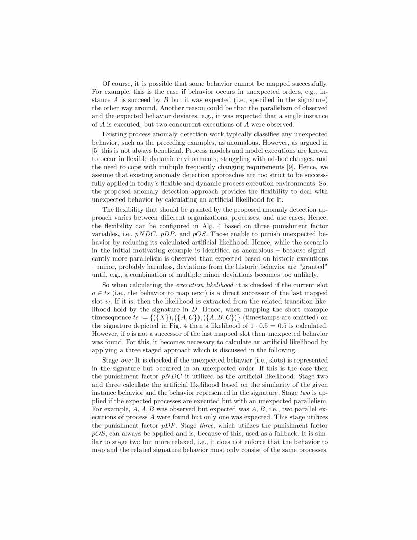
Algorithm matchSig(signature G = (V,D), dummy vertex vd representing the processwhich G was generated for, time sequence ts holding behavior to map, punishment factorspNDC, pDP, pOS ∈ (0; 1])

Result: calculated likelihood lh ∈ R>0 for tslh := 1; vl := vd // behavior likelihood lh and most recent signature vertex vlforeach o ∈ ts // individually for each slot do

lh′ := {d.tl ∈ D|d.v1 = vl ∧ d.v2 = o.N}P := {(v′, sim)|v′ ∈ V ; sim :=

|v′4o.N||v′|+|o.N| , ∀a ∈ o.N, ∃b ∈ v

′; a = b}

MS := {(v′, sim)|v′ ∈ V ; sim :=|v′4o.N||v′|+|o.N|}// 4 notates a symmetric difference

if lh′ = ∅ // unexpected behavior was found thenif o.N ∈ V // stage one: exact behavior is present in the signature then

vl := o.N ; lh := lh · pNDCelse if P 6= ∅ // stage two: present but different parallelism then

min := {p1|p1 ∈ P ; ∀p2 ∈ P, p1.sim ≤ p2.sim}0vl := min.v; lh := lh · (1−min.sim) · pDP

else// stage three: fallback if one and two are not applicable

min := {ms1|ms1 ∈MS; ∀ms2 ∈MS,ms1.sim ≤ ms2.sim}0vl := min.v; lh := lh · (1−min.sim) · pOS

elsevl := o.N ; lh := lh · lh′0 // if the behavior is expected

return lh// return likelihood lh of the behavior in ts

Algorithm 4: Likelihood for a time sequence ts based on a signature G

Of course, it is possible that some behavior cannot be mapped successfully.For example, this is the case if behavior occurs in unexpected orders, e.g., in-stance A is succeed by B but it was expected (i.e., specified in the signature)the other way around. Another reason could be that the parallelism of observedand the expected behavior deviates, e.g., it was expected that a single instanceof A is executed, but two concurrent executions of A were observed.

Existing process anomaly detection work typically classifies any unexpectedbehavior, such as the preceding examples, as anomalous. However, as argued in[5] this is not always beneficial. Process models and model executions are knownto occur in flexible dynamic environments, struggling with ad-hoc changes, andthe need to cope with multiple frequently changing requirements [9]. Hence, weassume that existing anomaly detection approaches are too strict to be success-fully applied in today’s flexible and dynamic process execution environments. So,the proposed anomaly detection approach provides the flexibility to deal withunexpected behavior by calculating an artificial likelihood for it.

The flexibility that should be granted by the proposed anomaly detection ap-proach varies between different organizations, processes, and use cases. Hence,the flexibility can be configured in Alg. 4 based on three punishment factorvariables, i.e., pNDC, pDP , and pOS. Those enable to punish unexpected be-havior by reducing its calculated artificial likelihood. Hence, while the scenarioin the initial motivating example is identified as anomalous – because signifi-cantly more parallelism is observed than expected based on historic executions– minor, probably harmless, deviations from the historic behavior are “granted”until, e.g., a combination of multiple minor deviations becomes too unlikely.

So when calculating the execution likelihood it is checked if the current sloto ∈ ts (i.e., the behavior to map next) is a direct successor of the last mappedslot vl. If it is, then the likelihood is extracted from the related transition like-lihood hold by the signature in D. Hence, when mapping the short exampletimesequence ts := {({X}), ({A,C}), ({A,B,C})} (timestamps are omitted) onthe signature depicted in Fig. 4 then a likelihood of 1 · 0.5 = 0.5 is calculated.However, if o is not a successor of the last mapped slot then unexpected behaviorwas found. For this, it becomes necessary to calculate an artificial likelihood byapplying a three staged approach which is discussed in the following.

Stage one: It is checked if the unexpected behavior (i.e., slots) is representedin the signature but occurred in an unexpected order. If this is the case thenthe punishment factor pNDC it utilized as the artificial likelihood. Stage twoand three calculate the artificial likelihood based on the similarity of the giveninstance behavior and the behavior represented in the signature. Stage two is ap-plied if the expected processes are executed but with an unexpected parallelism.For example, A,A,B was observed but expected was A,B, i.e., two parallel ex-ecutions of process A were found but only one was expected. This stage utilizesthe punishment factor pDP . Stage three, which utilizes the punishment factorpOS, can always be applied and is, because of this, used as a fallback. It is sim-ilar to stage two but more relaxed, i.e., it does not enforce that the behavior tomap and the related signature behavior must only consist of the same processes.

Imagine that the slot o with o.N := {A,A} should be mapped to a signaturewhich only consist of A as the expected behavior. Because, the observed {A,A}and the expected {A} behavior is different the slot cannot be found in thesignature. Hence the proposed approach falls back to stage two of the artificial

likelihood calculation. So the likelihood is calculated as |{A}4{A,A}||{A}|+|{A,A}| 7→

13 =

0.3 so that the final artificial likelihood becomes (1 − 0.3) · 0.8 = 0.53 when apunishment factor pDP of 0.8 is used.

The reference likelihood lr is calculated based on logged historic executionsin L that show comparable behavior to the given behavior (i.e., given instanceexecution behavior to analyze for anomalies). In this case comparable meansthat the time sequence describing the given behavior and the time sequences de-scribing the historic behavior hold similar slots. For this the presented approachto measure the similarity between two slots (i.e., for artificial likelihood calcula-tion, cf. Alg. 4) is generalized and applied on the historic time sequences whichwere mined from L during the signature generation. The k ∈ (0, 1] percent mostsimilar historic time sequences are subsequently compared with the signatureG using Alg. 4. Finally the lowest likelihood found during that comparisons isutilized as the reference likelihood lr. If le < lr then the given behavior (i.e., thebehavior that is analyzed for anomalies) is identified as anomalous. This bearstwo advantages: Executions in L are never identified as anomalous and the flex-ibility which was historically observed for the process under analysis, and whichis because of this stored in L, is taken into account during anomaly detection.

5 Evaluation

The evaluation utilizes real life process execution logs from multiple domainsand artificially generated anomalies in order to assess the anomaly detectionperformance and feasibility of the proposed approach. It was necessary to gen-erate artificial anomalies as information about real anomalies are not providedby the log sources. The utilized logs were taken from the BPI Challenge 20151

and 20172 (BPIC5 and BPIC7), and Higher Eduction Processes (HEP), cf. [13].

The BPIC5 logs hold 262,628 execution events which origin from 5,649 in-stances and 398 activities. The logs cover the processing of building permitapplications at five (BIPC5 1 to BPIC5 5) Dutch building authorities between2010 and 2015. In comparison the BPIC7 logs hold 1,202,267 events from 31,509instances, recorded in 2016 and 2017, which focused on loan application manage-ment. The HEP logs contain 28,129 events, 354 execution traces (i.e., instances),and 147 activities – recorded from 2008 to 2011. Each trace holds the interactionsof a student with an e-learning platform (e.g., exercise uploads). The interactionsare recorded individually for each academic year 7→ HEP 1 to HEP 3. All logs

1 http://www.win.tue.nl/bpi/2015/challenge—DOI: 10.4121/uuid:31a308ef-c844-48da-948c-305d167a0ec1

2 http://www.win.tue.nl/bpi/doku.php?id=2017—DOI: 10.4121/uuid:5f3067df-f10b-45da-b98b-86ae4c7a310b

(i.e., BPIC and HEP) contain sufficient details to apply the proposed approach(e.g., instance execution events and relevant timestamps).

The logs were evenly and randomly separated into training (for signaturegeneration) and test data (for the anomaly detection performance evaluation).A tenth of the test data was mutated by one (out of four) randomly chosen muta-tors (we regard this amount as being sufficient, cf. [4]). This enables to generatelabeled non-anomalous (i.e., non-mutated) and anomalous (i.e., mutated) testdata entries, i.e., to determine if both behavior “types” are correctly differ-entiated by the proposed approach. The applied four mutators generate multiinstance anomalies that cannot be detected by existing single business processinstance focused anomaly detection work, hence, a comparison with such existingwork is not possible: a) Parallel Executions – a process execution is duplicatedso that it occurs in parallel; and b) Sequential Executions – a process executionis duplicated so that occurs in a sequential order; and c) Execution Order – theprocess execution order is randomly changed; and d) New or Missing Process –new process executions are artificially added or recorded executions are removed.

The mutators were adapted and extended from our work in [4] – which wasassessed by security experts as being realistic. It was chosen to combine multiplemutators to represent that real life anomalies are diverse and affect differentaspects of process executions. In addition, the applied strategy also evaluatesthe proposed handling of unexpected execution behavior. This is, because thetest data (in its mutated but also non-mutated form) contains behavior that isnot represented in the training data (e.g., manual ad-hoc changes). The followingresults consist of the average of 100 evaluation runs – individually for each logfile – to even out the randomness in the data separation and mutation.

Metrics and Evaluation The feasibility of the presented anomaly detectionapproach is analyzed. For this, the training data is utilized to construct signa-tures which are applied on the test data to differentiate between known ran-domly mutated (i.e., anomalous) the known non-mutated (i.e., non-anomalous)test data entries. This enables to collect four key performance indicators: TruePositive (TP) and True Negative (TN) represent data entries that were cor-rectly identified as anomalous (TP) or non-anomalous (TN). In comparison,False Positive (FP) and False Negative (FN) represent data entries which wereincorrectly identified as anomalous (FP) or non-anomalous (FN). For example,FP counts non-anomalous test data entries which were incorrectly identified asbeing anomalous. Based on this performance indicators three standard metricsare calculated for each log file (i.e., BPIC5 1-5, BPIC7, and HEP 1-3):

a) Precision P = TP/(TP + FP ) – indicates if the identified anomaloustest data entries were in fact anomalies; and b) Recall R = TP/(TP + FN)– indicates if anomalies were “missed”, i.e., not identified; and c) AccuracyA = (TP + TN)/(TP + TN + FP + FN) – provides a general anomaly de-tection performance overview; TP, TN,FP, FN ∈ N>0; P,R,A ∈ [0; 1].

For this paper we assume that the number of False Positives (FP) or Nega-tives (FN) should be low while the number of True Positives (TP) or Negatives(TN) should be high, i.e., the accuracy becomes close to one. In addition the

Fβ-measure, Eq. 1, is applied because it provides a configurable harmonic meanbetween Precision (P) and Recall (R), cf. [8]. Hereby, β controls the balancebetween P and R. So, if β = 1 then a harmonic mean between P and R is calcu-lated. In comparison a β < 1 results in a precision and a β > 1 in a recall-orientedresult. F0.5,F1,F1.5-measures were used to present the evaluation results.

Fβ =(β2 + 1) · P ·Rβ2 · P +R

(1)

Results The results were generated based on BPIC 2015/2017 and HEP processexecution logs and a publicly available proof-of-concept implementation of thepresented approach: https://github.com/KristofGit/MultiInstanceAnomaly.The implementation calculated a signature in minutes (i.e., about 2 minutes onaverage) and required only seconds (i.e., below 3 seconds on average) to identifya test data entry as anomalous or non-anomalous on a standard 2.6 Ghz IntelQ6300 CPU with 8 GB of RAM. Of course, the signatures can be reused, i.e.,calculated once and subsequently applied in order to analyze multiple follow-ing process executions. Moreover, the presented approach can be concurrentlyapplied to analyze multiple instances in parallel. This suggests an applicabilityeven on larger process repositories and execution logs.

Primary tests were applied to identify appropriate configuration values forthe presented approach. The punishment factors for unexpected behavior wereset to pNDC = 0.60 (known behavior but unexpected order), pDP = 0.40(known behavior but unexpected parallelism), pOS = 0.30 (unknown behavior).A lower punishment factor results in a stronger punishment. So for example,pDP is higher than pOS because the latter is only utilized if completely unknownexecution behavior is observed. In comparisons the former is applied if “only”an unexpected parallel execution occurred. This is the case, for example, if threeparallel executions of process A were observed but only two were expected. As arule of thumb it can be assumed that a higher punishment improves on the TP/FN side while having a negative impact on the TN/FP performance indicators.A similar conclusion can be drawn for k = 0.3, i.e., the percentage of similar timesequences for reference likelihood generation purposes. When k is increased thenthe proposed approach becomes more relaxed because the reference likelihoodtypically decreases, i.e., anomalous instances are more likely “overlooked”.

A window size ws of 4 (BPIC) and 20 (HEP) was utilized. Hereby, the differ-ent ws values compensate that the log sources (e.g., BPIC or HEP) store eventswith a different density (i.e., the BPIC logs cover more events at the same times-pan than the HEP logs). The log dependent ws-value ensures that the generatedsignatures represent a roughly comparable amount of process execution eventsfor all log sources. Finally, a noise prevention value of c = 8 was utilized, i.e., aslot – either original or aggregated – has to cover at least 8 activity executionsto not be recognized as volatile or noise and being removed. The chosen valueswere successfully applied on different processes and domains. Hence, we assumethat they can be applied as a valid starting point for future optimizations inscenarios and domains which were not covered by the presented evaluation.

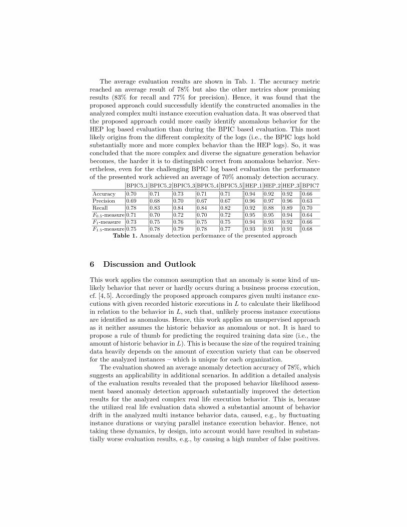
The average evaluation results are shown in Tab. 1. The accuracy metricreached an average result of 78% but also the other metrics show promisingresults (83% for recall and 77% for precision). Hence, it was found that theproposed approach could successfully identify the constructed anomalies in theanalyzed complex multi instance execution evaluation data. It was observed thatthe proposed approach could more easily identify anomalous behavior for theHEP log based evaluation than during the BPIC based evaluation. This mostlikely origins from the different complexity of the logs (i.e., the BPIC logs holdsubstantially more and more complex behavior than the HEP logs). So, it wasconcluded that the more complex and diverse the signature generation behaviorbecomes, the harder it is to distinguish correct from anomalous behavior. Nev-ertheless, even for the challenging BPIC log based evaluation the performanceof the presented work achieved an average of 70% anomaly detection accuracy.

BPIC5 1 BPIC5 2 BPIC5 3 BPIC5 4 BPIC5 5 HEP 1 HEP 2 HEP 3 BPIC7

Accuracy 0.70 0.71 0.73 0.71 0.71 0.94 0.92 0.92 0.66

Precision 0.69 0.68 0.70 0.67 0.67 0.96 0.97 0.96 0.63

Recall 0.78 0.83 0.84 0.84 0.82 0.92 0.88 0.89 0.70

F0.5-measure 0.71 0.70 0.72 0.70 0.72 0.95 0.95 0.94 0.64

F1-measure 0.73 0.75 0.76 0.75 0.75 0.94 0.93 0.92 0.66

F1.5-measure 0.75 0.78 0.79 0.78 0.77 0.93 0.91 0.91 0.68Table 1. Anomaly detection performance of the presented approach

6 Discussion and Outlook

This work applies the common assumption that an anomaly is some kind of un-likely behavior that never or hardly occurs during a business process execution,cf. [4, 5]. Accordingly the proposed approach compares given multi instance exe-cutions with given recorded historic executions in L to calculate their likelihoodin relation to the behavior in L, such that, unlikely process instance executionsare identified as anomalous. Hence, this work applies an unsupervised approachas it neither assumes the historic behavior as anomalous or not. It is hard topropose a rule of thumb for predicting the required training data size (i.e., theamount of historic behavior in L). This is because the size of the required trainingdata heavily depends on the amount of execution variety that can be observedfor the analyzed instances – which is unique for each organization.

The evaluation showed an average anomaly detection accuracy of 78%, whichsuggests an applicability in additional scenarios. In addition a detailed analysisof the evaluation results revealed that the proposed behavior likelihood assess-ment based anomaly detection approach substantially improved the detectionresults for the analyzed complex real life execution behavior. This is, becausethe utilized real life evaluation data showed a substantial amount of behaviordrift in the analyzed multi instance behavior data, caused, e.g., by fluctuatinginstance durations or varying parallel instance execution behavior. Hence, nottaking these dynamics, by design, into account would have resulted in substan-tially worse evaluation results, e.g., by causing a high number of false positives.

Note, a large amount of false positives could harm an organization’s performance,e.g., through process executions which are unnecessarily halted or terminated.

The presented approach determines process executions as anomalous basedon their relations to other preceding, succeeding, or simultaneous instances. Incomparison to existing work this is a rather big picture focused approach which,by purpose, ignores more fine granular details (e.g., which resource has executedan activity or what data was exchanged between two activities). Hence, in fu-ture work we will strive to combine both worlds. Hereby, multiple views on theinstance behavior can be taken into consideration to identify diverse and com-plex anomalous behavior. We assume this as necessary to identify inside threatsthat actively hide their malicious intentions. Moreover, we will assess the appli-cability of the proposed approach to analyze complex dynamic parallel activityexecutions. Finally, we will strive to integrate correlation features to respectcontextual aspects, e.g., by adding support for filters to analyze only processinstances that meet specific conditions (e.g., based on the involved resources).

References

1. Allen, J.F.: Maintaining knowledge about temporal intervals. ACM 26(11), 832–843 (1983)

2. Atallah, M., Szpankowski, W., Gwadera, R.: Detection of significant sets of episodesin event sequences. In: Data Mining. pp. 3–10. IEEE (2004)

3. Bezerra, F., Wainer, J., van der Aalst, W.M.: Anomaly detection using processmining. In: Enterprise, Business-Process and Information Systems Modeling, pp.149–161. Springer (2009)

4. Bohmer, K., Rinderle-Ma, S.: Automatic signature generation for anomaly detec-tion in business process instance data. In: Business Process Modeling, Developmentand Support. pp. 196–211. Springer (2016)

5. Bohmer, K., Rinderle-Ma, S.: Multi-perspective anomaly detection in business pro-cess execution events. In: COOPIS. pp. 80–98. Springer (2016)

6. Bohmer, K., Rinderle-Ma, S.: Anomaly detection in business process runtime be-havior – challenges and limitations. arXiv (2017)

7. Chaoji, V., Rastogi, R., Roy, G.: Machine learning in the real world. VLDB En-dowment 9(13), 1597–1600 (2016)

8. Chinchor, N., Sundheim, B.: Muc-5 evaluation metrics. In: Message understanding.pp. 69–78. Computational Linguistics (1993)

9. Fdhila, W., Rinderle-Ma, S., Knuplesch, D., Reichert, M.: Change and compliancein collaborative processes. In: Services Computing. pp. 162–169. IEEE (2015)

10. Gupta, M., Gao, J., Aggarwal, C.C., Han, J.: Outlier detection for temporal data:A survey. Knowledge and Data Engineering 26(9), 2250–2267 (2014)

11. de Leoni, M., van der Aalst, W.M., Dees, M.: A general process mining frameworkfor correlating, predicting and clustering dynamic behavior based on event logs.Information Systems 56, 235–257 (2016)

12. Rogge-Solti, A., Kasneci, G.: Temporal anomaly detection in business processes.In: Business Process Management. pp. 234–249. Springer (2014)

13. Vogelgesang, T., et al.: Multidimensional process mining: Questions, requirements,and limitations. In: CAISE Forum. pp. 169–176. Springer (2016)

14. Wieringa, R.J.: Design science methodology for information systems and softwareengineering. Springer (2014)