Applied Mathematical Sciences, Vol. 8, 2014, no. 15, 733 - 742

HIKARI Ltd, www.m-hikari.com http://dx.doi.org/10.12988/ams.2014.312690

Multi Flying Vehicle Control for Saving Fuel

R. Heru Tjahjana

Department of Mathematics

Faculty of Science and Mathematics, Diponegoro University

Jl. Prof. Sudarto, SH Tembalang, Semarang 50275 Indonesia

Priyo Sidik Sasongko

Department of Informatics Engineering

Faculty of Science and Mathematics, Diponegoro University

Jl. Prof. Sudarto, SH Tembalang, Semarang 50275 Indonesia

Copyright ©2014 R. Heru Tjahjana and Priyo Sidik Sasongko. This is an open access article

distributed under the Creative Commons Attribution License, which permits unrestricted use,

distribution, and reproduction in any medium, provided the original work is properly cited.

Abstract

This paper describes flying multi-vehicle control strategies and its benefit for saving fuel. Exposition starts from inspiration of flying multi-vehicle in daily life. Furthermore, from model of single flying vehicle, we construct the model of multi-vehicle and cost functional model that describe the state of the cost to be met the flying vehicle. The flying multi-vehicle control designed with optimal control strategy. The design of optimal control is done through the Pontryagin Maximum Principle, brings the model to a system of equations consisting of state equations and costate equations. In the system of states equations, each having initial and final condition, in the costate equations system has no requirements at all. The next problem is converted to the initial value problem and search for the approximate initial condition equation of costate equations system which has no requirements using a modified method of steepest descent. Thus, the control of multi-vehicle successfully performed and the simulation results presented on the results and discussion section. In addition, we also calcute the fuel which used by multi-vehicle, compared by the fuel which used by each vehicle in solo flying. The result can be conclude that the fuel more efficient if the flying vehicles in formation flying.

Keywords: flying vehicle, multi-vehicle, fuel saving

734 R. Heru Tjahjana and Priyo Sidik Sasongko

1 Introduction

Swarming behavior is naturally clustered behavior shown by animals and occurs

on land, sea, or air (Liu and Passino, 2000). Example of the phenomenon of

swarming on the ground is a bunch of hyenas in pursuit of prey. With swarming,

pursuit of prey by a bunch of hyenas are more likely to get results than a hyena

who pursue their prey alone (Wiesel, 2006). Example of the phenomenon of

swarming in the ocean occurs in herring horde. When swimming, herring fish

releasing little mucus to reduce turbulence, consequently herring fish that swim

behind others will benefit because the energy required to fight the turbulence

becomes smaller (Huse et al., 2002). Bunch of wild geese when flying together is

an example of swarming phenomenon that occurs in the air. Swarming

phenomenon with the formation of this particular motion is specifically referred to

as flocking. Flocking phenomena that happens to a group of geese forming

inverted V formation. With inverted V formation, geese form a particular vortex

field, the birds of the most swan as a "leader" and the aerodynamic gain a greater

distance to fly farther and higher cruising speed (Seiler, 2003).

Beside shown by the animals, flocking phenomenon also appears in the transport

vehicle. In carrying out its mission, aircraft fly together. The fighter planes

engaged with leading aircraft as a leader do flocking with inverted V-formation

will give the effect of better efficiency in terms of fuel and the speed of the

aircraft are moving solo (Thien et al., 2007). The paper authored by Thien et al.

(2007) shows the efficiency through wing of aircraft design. In conducting its

operations, naval warship convoy consisting of aircraft carriers and other small

ships sail together. Moving ships clustered with certain formations will provide

better communication networks and efficient in monitoring the surrounding

conditions (Borhaug et al., 2006). The next studies related to multi-vehicle control,

published by Børhaug et al., (2006), Arrichiello et al., (2006), Gazi et al., (2007),

Breivik et al.,(2008), Ahmadzadeh et al., (2009) , Moshtagh et al., (2009), Shi et

al. (2009), Su et al. (2009), but these papers do not discuss about the flying

vehicle.

The recent research on multi flying vehicle that has been published, for example,

by Michael, et al. (2011), which uses multi- vehicle flew for surveillance activities,

further Kaliappan, et al. (2011) examined the multi helicopter mini models are

used for the benefit of search and surveillance. The other research conducted by

Fink, et al. (2011) worked on controlling the flying robot lifting together. While

Turpin, et al. (2012) published their work on the spacecraft formation flying

quadrotors used to attack the opponent. The other publications authored by

Lindsey, et al. (2012) explored the quadrotors team together to build

three-dimensional objects.

Multi flying vehicle control for saving fuel 735

2 Multi Vehicle Model

Either in mathematics or in engineering, flight dynamics of the single vehicle can

be modeled in general as a model of non-linear dynamic system as follows

=f(x(t),u(t)). (1)

In equation (1), the state vector x contains the state variables that determine the

flying vehicle dynamics. In general, the state vector here is a vector that describes

the position and orientation of flying vehicle. Vector field f in equation (1)

contains something that explain the link between the state vector x and input or

control u. When construct as a model of multi-vehicle, then from equation (1) can

be presented as

=f1(x1(t),u1(t))

=f2(x2(t),u2(t))

(2)

=fk(xk(t),uk(t)).

In the system of equations (2), the dynamics of the first flying vehicle modeled by

the first equation, the second flying vehicle modeled by second equations, and

each row in the equation (2) describe a flying vehicle, until the last flying vehicle

modeled by the last row in equation (2).

In this paper, for single vehicle model we follow Zheng et al. (2008), specially

selected flight dynamics of the vehicle in the form of non-linear

{

(3)

as a specific form or a specific incident of equation (1), then the equation (3)

include the state vector x(t) =[x(t), y(t), and the input vector or control

vector u(t) =[ . The control is airspeed rate and is turn

rate. Zheng et al. (2008) use the model which describe in (3) to control three

flying vehicles track the given desired path. From the single vehicle dynamics can

be formed as a multi-agent multi vehicle models as special form of the system of

equations (2) as follows

{

{

(4)

736 R. Heru Tjahjana and Priyo Sidik Sasongko

{

In this paper, we consider the system with three flying vehicles, so from equation

(4) can be obtained the model of multi flying vehicle as follows

{

{

(5)

{

Next, discussed the cost functional model that makes the vehicle cannot move

away from each other, and does not collide with each other and also includes a

model that represents the fuel from the vehicle to fly together, which is a subject

of interest in this study. Functional model is generally the cost is as follows

∫

(6)

Note the cost functional (6), the functional J consists of two parts, namely g and h

term. The first part, g repulsion tribes and tribal tribes load pull, which makes the

vehicle does not collide with each other and fly less away from each other. The

second part, h rate includes the cost of parts that states total control of the vehicle

or can also be interpreted as a special energy that is directly proportional to fuel

the vehicle. Functional costs are presented in (6) is the most common functional

costs. When are specified, then the tribe tribes containing g repulsion and

attraction term can be presented as

∑

‖ ‖ ∑

(‖ ‖) (7)

In equation (7), the first term is the repulsion term, γ is the repulsion constants,

this term will make the flying vehicles do not collide with each other.

Furthermore the second term in equation (7) is the atrractor term, with μ is a

atrractor constant, the presence of these terms make the flying vehicles do not

moving away from each other. Thus, in more detail the functional costs generally

presented in (6) can be expressed in the following equation

∫

∑

‖ ‖ ∑

(‖ ‖) ∑

‖ ‖ (8)

In equation (8), is actually still common also, because of the many vehicles that

set is k vehicles, whereas in this study was applied to the three vehicles then more

precisely model the cost functional used is as follows

Multi flying vehicle control for saving fuel 737

∫

∑

‖ ‖ ∑

(‖ ‖) ∑

‖ ‖ (9)

The third term in equation (9) is an energy tribe specific physical controls can be

claimed as something that is directly proportional to the fuel. In this paper, we

assume that airspeed rate or directly proportional to the fuel which used.

3 Simulation Result

The simulation starts with describe the simulation scenarios. Scenario of the

simulation is done to control three flying vehicles that flew from a particular

position and orientation toward a certain position by the end of orientation as a

goal. The vehicles are not allowed to move away and not collide. The

eexpectation of this simulation is with perform flying together, the fuel being used

more efficiently. Control design of the vehicle using the optimum control by

utilizing the Pontryagin Maximum Principle. From multi-vehicle model that

descrideb in (5) and the cost functional that defined in (9) can be obtained

Hamilton function. From the Hamilton function can be obtained the Hamiltonian

system. The Hamiltonian system consists of the state system and auxiliary system

or costate system. For optimality conditions, the Hamiltonian differentiated into

each control variable and then make the term equal to zero, the results obtained

control equations for each vehicle. Then, the equation of the vehicle control

system is put back into Hamilton System, and a system of differential equation is

obtained.

In this paper, the simulation is done with the initial condition

x(0)=[x1(0), x2(0), x3(0), y1(0), y2(0), y3(0), 1(0), 2(0), 3(0)]

=[7,3,9,7,5,3, /4, /4, /4]

and the final condition

x(1)=[x1(1),x2(1),x3(1),y1(1),y2(1),y3(1), 1(1), 2(1), 3(1)]

=[13,9,15,13,10,9,– /7,– /7,– /7].

Simulation is done with matlab software. In the simulation cannot be done with

just a simple as relying on software alone. In the next step, difficulties appear on

the system of differential equations, exactly, the system has excessive condition.

Usually on issues of differential equations encountered a problem with the

differential equation initial conditions, or the final terms problems, or problems

with initial and final conditions as well, but in the completion of this simulation is

obtained half of the members of Hamiltonian systems, systems equation of state

has the initial and final conditions, but the costate variables do not have any

conditions. This difficulty is resolved by changing the problem to the initial value

problem, and the approximation for initial value of the costate equations following

Algorithm 1 as follows.

Algorithm 1

Data

738 R. Heru Tjahjana and Priyo Sidik Sasongko

Step 0 : set i = 0

Step 1 : Calculate the search direction

Stop

Step 2 : Calculate the step- size ( )

Step 3 : Set

Substitution i with i +1 Go To Step 1.

The convergence of sequence go to the best approximation for

initial conditions of auxiliary state variables or costate variables shown in

Theorem 1 below.

Theorem 1

Suppose F has a derivative and { }

is the sequence constructed by algorithm

1, then for each point of convergence for q* and { }

will satisfy

Proof:

Suppose that sequence converges to and assume

. Let Lipschitz constants for on the ball with center

and the radius denoted by ( . Suppose again ( ] such

that

‖ ‖

‖ ‖

for every With the mean value theorem in calculus, then for an

applies

( ) ( ) ( ) [⟨ ( ) ( ) ⟩]

( ) ( )

( )

Note that

( ) ‖ ( )‖‖ ‖

Because satisfy the Lipschitz condition then

( ) ( ) ‖ ‖

For obtained

( ) ( ) ‖ ‖ ,

and consequently

( ) ( ) ‖ ( )‖‖ ‖ ‖ ‖ . (10)

Minimum of the right hand side of inequality (10) occurred in

‖ ‖

Multi flying vehicle control for saving fuel 739

with

‖ ‖

.

Suppose

= { }

and defined

‖ ‖ .

As a result – Since the value of the right hand side of inequality (10) for

‖ ‖ must be greater than the minimum value of the left hand side

inequality (10) for λ, then applies be

( ) ( ) (11)

Since sequence { ( )}

monotonically down and because F continuous

function, then the sequence { ( )} converges toward Follow the

monotonous nature of the line, then for i go to apply ∞ ( ) to . On the

other side of the inequality (11) to get, for i go to ∞ then apply ( ) to -∞. Up

here obtained two opposites or contradiction. Then the presuppositions must be

negated and we obtain that .

Utilize Algorithm 1, the best approximation for initial values of costates variables

are obtained. The method which proposed in Algoritm 1 here, more general than

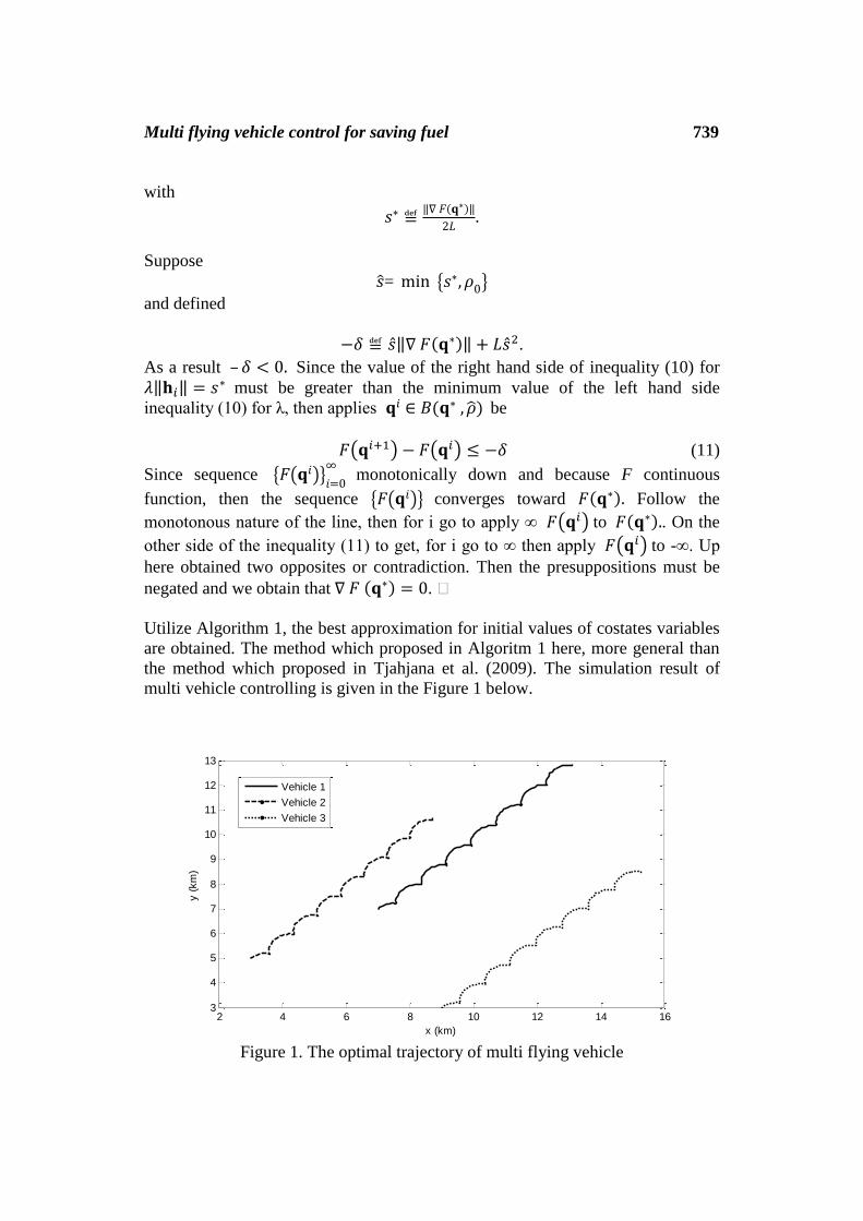
the method which proposed in Tjahjana et al. (2009). The simulation result of

multi vehicle controlling is given in the Figure 1 below.

Figure 1. The optimal trajectory of multi flying vehicle

2 4 6 8 10 12 14 163

4

5

6

7

8

9

10

11

12

13

x (km)

y (

km

)

Vehicle 1

Vehicle 2

Vehicle 3

740 R. Heru Tjahjana and Priyo Sidik Sasongko

In Figure 1, one can see that the vehicles were controlled to move meet the

simulation scenarios, from the trajectory of the vehicles can be seen that the

vehicles do not collide with each other. The vehicles also do not move away from

each other. This result indicates that the costs functional (9) described above, can

work well.

Furthermore, use the third term of functional costs functional (9) by using the

airspeed rate that associated with the fuel used for each vehicles, the fuel

used can be calculated. The fuel which used by the vehicles on the simulation

above can be calculated as follows, when the vehicle flying solo fuel that must be

spent by each vehicle is 9.4317e+004 volume units. Referring Ray, et al. (2002)

which states that the formation would reduce the inhibition of the (drag) by 20 %,

then the reduction in fuel or fuel savings can be claimed to be comparable with

the subtraction of this drag, when the vehicle flew together, the fuel which used

by each vehicle is 7.5454e+004 volume units.

4 Conclusion

Respectively associated with the process undertaken this publication is as follows,

from a single flying vehicle models, and mathematical modeling can be done

flying multivehicle. Furthermore, with the task of setting of the vehicle is flying

together with the formation, no collisions and not away from each other, then

drafted a functional model of the cost. From multi-vehicle models and functional

models can be obtained cost function which can then be expressed in Hamiltonian

Systems. By utilizing the Pontryagin Maximum Principle, obtained the over

determined system of differential equations. The strategy to solve this problem,

performed by bringing the problem to the completion of the initial value problem,

and apply Algorithm 1. Next, the control problem multi-vehicle successfully

satisfies the simulation scenario. Furthermore, the calculation of fuel have shown

that the fuel used to travel the same distance, when the vehicle flew alone

compared with when the vehicle flew in V-formation, the results show that the

fuel used in the formation more efficient or smaller than if the vehicle fly in Solo.

Acknowledgements. This research was funded by The Goverment of Republic of

Indonesia, throgh DIPONEGORO UNIVERSITY FUNDAMENTAL BOPTN

2013 RESEARCH GRANT, under contract number 302a-11/UN7.5/LT/2013.

References

[1] A. Ahmadzadeh, N. Motee, A. Jadbabaie and G. Pappas, Multi-vehicle path

planning in dynamically changing environments, Proceeding of IEEE

International Conference on Robotics and Automation, (2009), 2449-2454.

Multi flying vehicle control for saving fuel 741

[2] E. Børhaug, A. Pavlov, R. Ghabcheloo, K. Pettersen, K., A. Pascoal and C.

Silvestre, Formation control of underactuated marine vehicles with

communication constraints, Proceeding of IFAC Conference on Manuevering

and Control of Marine Craft, Lisbon, Portugal (2006).

[3] F. Arrichiello, S. Chiaverini, and T.I Fossen, Formation Control of Marine

Surface Vessels using the Null-Space-Based Behavioral Control, Lecture

Notes in Control and Information Systems series, Springer-Verlag, Vol. 336,

(2006).

[4] G. Huse, S. Railsback and A. Ferno, Modeling changes in migration pattern

of herring: collective bahaviour and nerical domination, Journal of Fish

Biology, 60, (2002), 571 - 582.

[5] H. Shi, L.Wang and T. Chu, Flocking of multi-agent systems with a

dynamic virtual leader, International Journal of Control, 82, (2009). 43-58.

[6] H. Su, X. Wang and G.Cheng, A Connectivity-preserving flocking

algorithm for multi-agent systems based only on position measurements,

International Journal of Control, 82, (2009), 1334-1343.

[7] H. Tjahjana, I. Pranoto, H. Muhammad and J. Naiborhu, On The Optimal

Control Computation of Linear Systems, Journal of the Indonesian

Mathematical Society, 15, (2009), 13-20.

[8] I. Weisel, Predatory and Foraging Behaviour of Brown Hyenas at cape fur

Seal colonies, Ph.D. Thesis, University of Hamburg, Germany, 2006.

[9] J. Fink, N. Michael, S. Kim and V. Kumar, Planning and Control for

Cooperative Manipulation and Transportation with Aerial Robots, The

International Journal of Robotics Research, 30, (2011), 324-334.

[10] M. Breivik, V.E. Hovstein, and T.I Fossen, Ship Formation Control: A

Guided Leader-Follower Approach, Proceeding of IFAC World Congress

Seoul (2008).

[11] M. Turpin, N. Michael, and V. Kumar, Trajectory design and control for

aggressive formation flight with quadrotors, Autonomous Robots, 33, (2012),

143-156.

742 R. Heru Tjahjana and Priyo Sidik Sasongko

[12] N. Michael, E.Stump and M.K Kartik, Persistent Surveillance with a

Team of MAVs, Proceeding of International Conference on Intelligent

Robots and Systems, San Francisco, CA, USA, (2011), 2708-2714.

[13] N. Moshtagh, N. Michael, A. Jadbabaie and K. Daniilidis, Vision-Based,

Distributed Control Laws for Motion Coordination of Nonholonomic Robots,

IEEE Transactions on Robotics, 25, (2009), 851-860.

[14] P. Seiler, A. Pan and K.Hedrick, A systems interpretation for observations

of bird v-formations, J. Theory Biology, 59221, (2003), 279 - 287.

[15] Q. Lindsey, D. Mellinger and V. Kumar, Construction with quadrotor teams,

Autonomous Robots, 33, (2012), 323-336.

[16] R.J. Ray, B. R. Cobleigh, M. J. Vachon and C.S. John, Flight Test

Techniques Used To Evaluate Performance Benefits During Formation

Flight, NASA Dryden Flight Research Center, California, 2002.

[17] T.I. Fossen, Guidance and control, Lecturer Note, Norwegian University of

Science and Technology, Trodheim, Norway, 2009.

[18] V. Gazi, B. Fidan, Y.S.Hanay and M.I. Koksal, Aggregation, foraging, and

formation control of swarms with non-holonomic agents using potential

functions and sliding mode techniques, Turk J Elec Engin, 15, No.2 (2007).

[19] V.K. Kaliappan, H. Yong, D. Min and A. Budiyono, Behavior-based

decentralized approach for cooperative control of a multiple small scale

unmanned helicopter, Proceeding of International Conference on Intelligent

Systems Design and Applications, Córdoba, Spain, (2011), 196-201.

[20] Y. Liu, and K. Passino, Swarm Intelligence: Literature Overview, The Ohio

State University, Neil Ave, Columbus, 2000.

[21] Z. Zheng, S.C. Spry and A.R. Girard, Leaderless Formation Control Using

Dynamic Extension and Sliding Control, Proceeding of The IFAC World

Conggres, 2008.

Received: December 10, 2013