Multi-Dimensional Scaling for Localization -...
66
Multi-Dimensional Scaling for Localization Traian E. Abrudan [email protected] . Instituto de Telecomunicac ¸ ˜ oes, Departamento de Engenharia Electrot ´ ecnica e Computadores, Universidade do Porto, Portugal Multi-Dimensional Scaling for Localization - GETA Winter School: Short Course on Wireless Localization, Ruka, Feb. 13–15, 2012 p1
Transcript of Multi-Dimensional Scaling for Localization -...

Multi-Dimensional Scaling forLocalization
Traian E. Abrudan
Instituto de Telecomunicacoes, Departamento de Engenharia
Electrotecnica e Computadores, Universidade do Porto, Portugal
Multi-Dimensional Scaling for Localization - GETA Winter School: Short Course on Wireless Localization, Ruka, Feb. 13–15, 2012 p 1
Outline• Motivation• Classical Position Estimation Algorithms
− Lateration, Angulation, mixed approaches• Multi-Dimensional Scaling (MDS) for estimating multiple positions
− Metric MDS− Weighted MDS (wMDS)− Distributed Weighted MDS (dwMDS)− Ordinal MDS (OMDS)− Extensions of the MDS algorithm
• Real-world results• Conclusions
Multi-Dimensional Scaling for Localization - GETA Winter School: Short Course on Wireless Localization, Ruka, Feb. 13–15, 2012 p 2
Motivation
• Goal: estimate the actual node position(s) using RF signals
• Often, range and/or angle estimates are available at the nodes
• They are subject to large errors, especially in indoors
• Algorithms that can tolerate errors are needed
Multi-Dimensional Scaling for Localization - GETA Winter School: Short Course on Wireless Localization, Ruka, Feb. 13–15, 2012 p 3
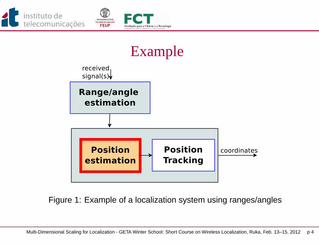
Example
Figure 1: Example of a localization system using ranges/angles
Multi-Dimensional Scaling for Localization - GETA Winter School: Short Course on Wireless Localization, Ruka, Feb. 13–15, 2012 p 4
Position estimation based on ranges and anglesRF-based techniques
• Ranges (i.e. distances) may be estimated based on− Received Signal Strength Indicator (RSSI) and calibrated
channel models− time-of-flight (ToF) measurements (one-way, round trip, time
differences, etc.) – suitable for Ultra-Wide Band (UWB) signals
• Angles may be estimated using− antenna arrays and Angle of Arrival (AoA) estimation techniques
• The most common approaches for position estimation are laterationand angulation
Multi-Dimensional Scaling for Localization - GETA Winter School: Short Course on Wireless Localization, Ruka, Feb. 13–15, 2012 p 5

Position estimation based on rangesLateration
x
y
d0,m
d1,m
d2,m
δ0,m = const.
δ1,m = const.
δ2,m = const.
Mm
N0 N1
N2
Figure 2: Tri-lateration with perfect range estimates
Multi-Dimensional Scaling for Localization - GETA Winter School: Short Course on Wireless Localization, Ruka, Feb. 13–15, 2012 p 6

Position estimation based on rangesLateration
x
y
d0,m
d1,m
d2,m
δ0,m = const.δ1,m = const.
δ2,m = const.
Mm
N0 N1
N2
Figure 3: Tri-lateration with over-estimated ranges (non-line-of-sight)
Multi-Dimensional Scaling for Localization - GETA Winter School: Short Course on Wireless Localization, Ruka, Feb. 13–15, 2012 p 7

Position estimation based on rangesLateration
• Consider a number of A anchor nodes N0, . . . , NA−1 whosepositions xa = [xa, ya]T , a = 0 . . . , A − 1 are known
• Let da,m =√
(xa − xm)2 + (ya − ym)2 = ‖xa − xm‖2 be theEuclidean distance between an anchor node Na, a = 0 . . . , A − 1,and the mth mobile node Mm, with coordinates xm = [xm, ym]T
• Let N0 be an arbitrary anchor node (reference node)• The differences of squared distances w.r.t. A0 are
d21,m− d2
0,m = x21−x2
0+y21−y2
0−2xm(x1−x0)−2ym(y1−y0)...
d2A−1,m− d2
0,m = x2A−1−x2
0+y2A−1−y2
0−2xm(xA−1−x0)−2ym(yA−1−y0)(1)
• Equations (1) may be rewritten in a convenient matrix-vector form
Multi-Dimensional Scaling for Localization - GETA Winter School: Short Course on Wireless Localization, Ruka, Feb. 13–15, 2012 p 8
Position estimation based on rangesLateration
2
x1−x0 y1−y0
...xA−1−x0 yA−1−y0
︸ ︷︷ ︸Hxy
[xm
ym
]
︸ ︷︷ ︸xm
=
x21−x2
0+y21−y2
0
...x2
A−1−x20+y2
A−1−y20
︸ ︷︷ ︸k
−
d21,m−d2
0,m
...d2
A−1,m−d20,m
.
︸ ︷︷ ︸∆d2
(2)
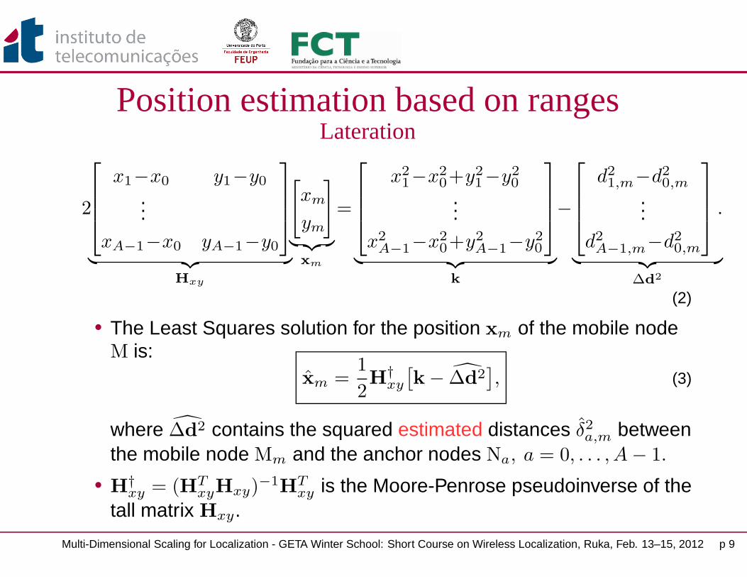
• The Least Squares solution for the position xm of the mobile nodeM is:
xm =1
2H
†xy
[k − ∆d2
], (3)
where ∆d2 contains the squared estimated distances δ2a,m between
the mobile node Mm and the anchor nodes Na, a = 0, . . . , A − 1.
• H†xy = (HT
xyHxy)−1H
Txy is the Moore-Penrose pseudoinverse of the
tall matrix Hxy.
Multi-Dimensional Scaling for Localization - GETA Winter School: Short Course on Wireless Localization, Ruka, Feb. 13–15, 2012 p 9

Position estimation based on rangesLateration
• In case some reliability information on the ranges is available, aWeighted Least Squares may be used:
xm =1
2(HT
xyWHxy)−1H
TxyW
[k− ∆d2
], (4)
• The weighting matrix W is a diagonal matrix, whose diagonalelements are w1, . . . , wA−1
• The reliability weights wa ∈ [0, 1], a = 0, . . . , A − 1
• The reference node N0 should be the one corresponding the mostreliable range estimate δ0,m, and w0 = 1
• The ranges may be determined either by using time-of-flight[HagAbrKoi09], or received signal strength [AbrPauBar11]
• If one-way ToF is used, tight synchronization among all nodes isrequired – round-trip ToF may be used instead [AbrHagKoi12]
Multi-Dimensional Scaling for Localization - GETA Winter School: Short Course on Wireless Localization, Ruka, Feb. 13–15, 2012 p 10

Position estimation using differential ToFHyperbolic Lateration
x
y
d0,m
d1,m
d2,m
t0− t1 = const.
t0− t2 = const.
Mm
N0 N1
N2
Figure 4: Hyperbolic tri-lateration with time-of-flight differences
Multi-Dimensional Scaling for Localization - GETA Winter School: Short Course on Wireless Localization, Ruka, Feb. 13–15, 2012 p 11
Position estimation using differential ToFHyperbolic Lateration
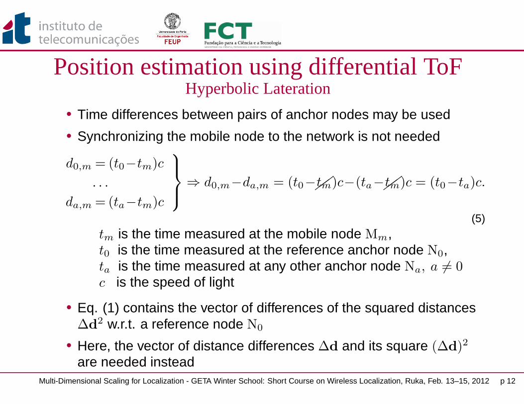
• Time differences between pairs of anchor nodes may be used• Synchronizing the mobile node to the network is not needed
d0,m = (t0−tm)c
. . .
da,m = (ta−tm)c
⇒ d0,m−da,m = (t0−tm)c−(ta−tm)c = (t0−ta)c.
(5)tm is the time measured at the mobile node Mm,t0 is the time measured at the reference anchor node N0,ta is the time measured at any other anchor node Na, a 6= 0c is the speed of light
• Eq. (1) contains the vector of differences of the squared distances∆d
2 w.r.t. a reference node N0
• Here, the vector of distance differences ∆d and its square (∆d)2
are needed insteadMulti-Dimensional Scaling for Localization - GETA Winter School: Short Course on Wireless Localization, Ruka, Feb. 13–15, 2012 p 12

Position estimation using differential ToFHyperbolic Lateration
• Rewrite (1) in a convenient way
(d1,m−d0,m)2
...(dA−1,m−d0,m)2
︸ ︷︷ ︸(∆d)2
+2d0,m
d1,m−d0,m
...dA−1,m−d0,m
︸ ︷︷ ︸∆d
= k−2Hxyxm. (6)
• The Least Squares solution for the position xm of the mobile nodeM is:
xm =1
2H
†xy
[k − 2d0,m∆d − (∆d)2
](7)
• A weighted approach may be used also in this case
Multi-Dimensional Scaling for Localization - GETA Winter School: Short Course on Wireless Localization, Ruka, Feb. 13–15, 2012 p 13
Position estimation using AoAsAngulation
x
y
angle origin
α0 α1
α2
Mm
N0
N1
N2
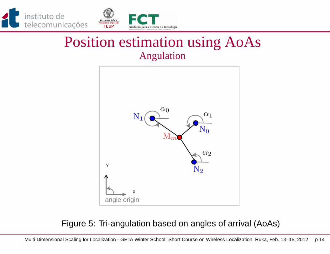
Figure 5: Tri-angulation based on angles of arrival (AoAs)
Multi-Dimensional Scaling for Localization - GETA Winter School: Short Course on Wireless Localization, Ruka, Feb. 13–15, 2012 p 14
Position estimation using AoAsAngulation
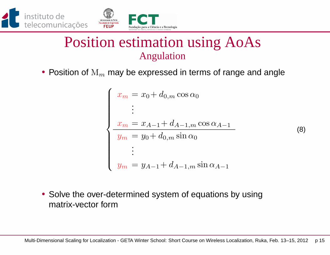
• Position of Mm may be expressed in terms of range and angle
xm = x0+ d0,m cosα0
...xm = xA−1+ dA−1,m cos αA−1
ym = y0+ d0,m sinα0
...ym = yA−1+ dA−1,m sinαA−1
(8)
• Solve the over-determined system of equations by usingmatrix-vector form
Multi-Dimensional Scaling for Localization - GETA Winter School: Short Course on Wireless Localization, Ruka, Feb. 13–15, 2012 p 15
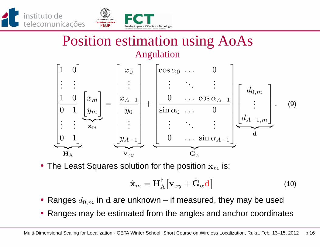
Position estimation using AoAsAngulation
1 0...
...1 0
0 1...
...0 1
︸ ︷︷ ︸HA
[xm
ym
]
︸ ︷︷ ︸xm
=
x0
...xA−1
y0
...yA−1
︸ ︷︷ ︸vxy
+
cosα0 . . . 0...
. . ....
0 . . . cosαA−1
sinα0 . . . 0...
. . ....
0 . . . sinαA−1
︸ ︷︷ ︸Gα
d0,m
...dA−1,m
︸ ︷︷ ︸d
. (9)
• The Least Squares solution for the position xm is:
xm = H†A
[vxy + Gαd
](10)
• Ranges d0,m in d are unknown – if measured, they may be used• Ranges may be estimated from the angles and anchor coordinates
Multi-Dimensional Scaling for Localization - GETA Winter School: Short Course on Wireless Localization, Ruka, Feb. 13–15, 2012 p 16
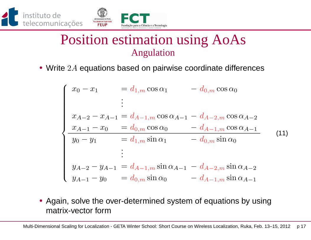
Position estimation using AoAsAngulation
• Write 2A equations based on pairwise coordinate differences
x0 − x1 = d1,m cosα1 − d0,m cosα0
...xA−2 − xA−1 = dA−1,m cosαA−1 − dA−2,m cosαA−2
xA−1 − x0 = d0,m cosα0 − dA−1,m cosαA−1
y0 − y1 = d1,m sinα1 − d0,m sinα0
...yA−2 − yA−1 = dA−1,m sinαA−1 − dA−2,m sinαA−2
yA−1 − y0 = d0,m sinα0 − dA−1,m sinαA−1
(11)
• Again, solve the over-determined system of equations by usingmatrix-vector form
Multi-Dimensional Scaling for Localization - GETA Winter School: Short Course on Wireless Localization, Ruka, Feb. 13–15, 2012 p 17
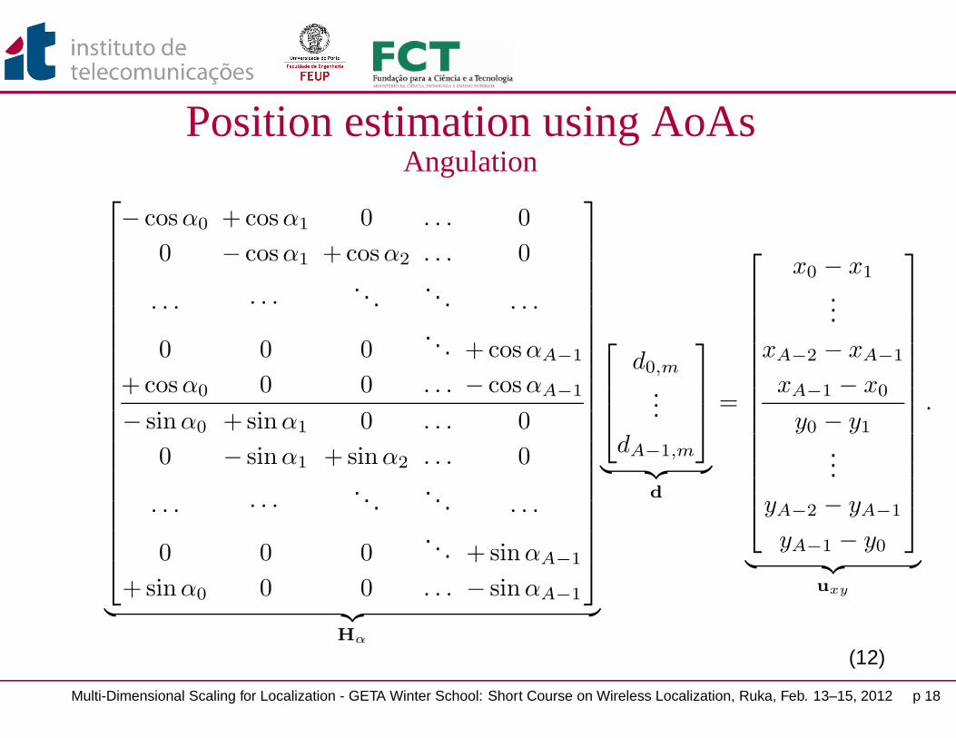
Position estimation using AoAsAngulation
− cosα0 + cosα1 0 . . . 0
0 − cosα1 + cosα2 . . . 0
. . . · · ·. . .
. . . . . .
0 0 0. . . + cosαA−1
+ cosα0 0 0 . . . − cosαA−1
− sinα0 + sinα1 0 . . . 0
0 − sinα1 + sinα2 . . . 0
. . . · · ·. . .
. . . . . .
0 0 0. . . + sinαA−1
+ sinα0 0 0 . . . − sinαA−1
︸ ︷︷ ︸Hα
d0,m
...dA−1,m
︸ ︷︷ ︸d
=
x0 − x1
...xA−2 − xA−1
xA−1 − x0
y0 − y1
...yA−2 − yA−1
yA−1 − y0
︸ ︷︷ ︸uxy
.
(12)
Multi-Dimensional Scaling for Localization - GETA Winter School: Short Course on Wireless Localization, Ruka, Feb. 13–15, 2012 p 18

Position estimation using AoAsAngulation
• The Least Squares solution for the ranges da,m in d is:
d = H†αuxy. (13)
• From Eqs. (10) and (13), the final node coordinates based onangles and anchor coordinates only are the following:
xm = H†A
[vxy + GαH
†αuxy
](14)
• Matrices Gα and Hα contain the estimated AoAs α0, . . . , αA−1
• Weighted approaches may also be used• Position estimators using combinations of angle and range
measurements may be derived as well (see e.g. [Sayed et al.])• Eq. (10) may also be used to fuse angular + range information:
xm = H†A
[vxy + Gαd
](15)
Multi-Dimensional Scaling for Localization - GETA Winter School: Short Course on Wireless Localization, Ruka, Feb. 13–15, 2012 p 19

Joint estimation of multiple positionsMulti-Dimensional Scaling (MDS)
• The techniques we have seen so far estimate the position of eachmobile node Mm independently, for m = 1, . . .N
• Relationship between unknown nodes was neglected• In some cases, it is desirable to estimate the positions of multiple
mobile nodes jointly
Problem:• How to estimate the spatial topology of the entire network of nodes
simultaneously?
Solution:• This problem may be efficiently solved by using the so called
Multi-Dimensional Scaling (MDS)
Multi-Dimensional Scaling for Localization - GETA Winter School: Short Course on Wireless Localization, Ruka, Feb. 13–15, 2012 p 20

Joint estimation of multiple positionsMulti-Dimensional Scaling (MDS)
• MDS is a modern technique [BorGro05] for visualizing data in amulti-dimensional space
• well-known in psychometry, econometrics, statistics, etc.• It uses pairwise “similarity” or “dissimilarity” measures• It orders multi-dimensional objects by mutual similarity (special
case of ordination)• Input data: pairwise (dis)similarities (e.g. distances)• Output data: set of coordinates (a local map)
MDSINPUT: pairwise distances
OUTPUT: Local map
Figure 6: Multi-dimensional scalingMulti-Dimensional Scaling for Localization - GETA Winter School: Short Course on Wireless Localization, Ruka, Feb. 13–15, 2012 p 21
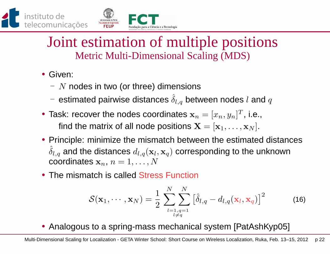
Joint estimation of multiple positionsMetric Multi-Dimensional Scaling (MDS)
• Given:− N nodes in two (or three) dimensions− estimated pairwise distances δl,q between nodes l and q
• Task: recover the nodes coordinates xn = [xn, yn]T , i.e.,find the matrix of all node positions X = [x1, . . . ,xN ].
• Principle: minimize the mismatch between the estimated distancesδl,q and the distances dl,q(xl,xq) corresponding to the unknowncoordinates xn, n = 1, . . . , N
• The mismatch is called Stress Function
S(x1, · · · ,xN ) =1
2
N∑
l=1,q=1
l6=q
N∑[δl,q − dl,q(xl,xq)
]2(16)
• Analogous to a spring-mass mechanical system [PatAshKyp05]Multi-Dimensional Scaling for Localization - GETA Winter School: Short Course on Wireless Localization, Ruka, Feb. 13–15, 2012 p 22

Joint estimation of multiple positionsMetric Multi-Dimensional Scaling (MDS)
• The pairwise squared distances (seen as functions of coordinates):
d2l,q(xl,xq) = ‖xl − xq)‖
22 = x
Tl xl − 2xT
l xq + xTq xq (17)
• The matrix of squared distances D2 = [d2
l,q]l,q can be written as:
D2 = ψ1
TN − 2XT
X + 1NψT , (18)
where 1N is an N × 1 vector of ones, and ψ = [xT1 x1, . . . ,x
TNxN ]T .
• Looks like equation (18) is impossible to solve – not really• Define the centering matrix H = IN − 1N1
TN/N
• Use the fact that H(ψ1TN + 1Nψ
T )H = ON , where ON in theN × N zero matrix
• By multiplying (18) with H in both sides, we get
HD2H = −2XT
X, (X = XH are the centered coordinates). (19)
Multi-Dimensional Scaling for Localization - GETA Winter School: Short Course on Wireless Localization, Ruka, Feb. 13–15, 2012 p 23

Joint estimation of multiple positionsMetric Multi-Dimensional Scaling (MDS)
• Define B =1
2HD
2H = X
TX. (20)
• Note that the rank of B is equal to two (or three, in 3 dimensions)
• The centered coordinates X = XH may be recovered byminimizing J (X) = ‖B − X
TX‖2
2
• closed-form solution by singular value decomposition (SVD):
X = Σ
1/21:2,1:2U
T1:2,1:N , (21)
where B = UΣVT is the SVD of B (Matlab notation was used to
select certain rows and columns).• U,V are N × N unitary matrices, i.e. U
TU = IN , V
TV = IN , and
they are called left/right singular vectors, respectively• Σ is a diagonal matrix whose diagonal elements σ1 ≥ . . . ≥ σN ≥ 0
are called singular values (IN is the N × N identity matrix)Multi-Dimensional Scaling for Localization - GETA Winter School: Short Course on Wireless Localization, Ruka, Feb. 13–15, 2012 p 24

Joint estimation of multiple positionsMetric Multi-Dimensional Scaling (MDS)
• Given exact range measurements, the entire spatial topology of thenetwork network is perfectly recovered
• The original distances are preserved exactly• Ambiguity: the coordinates are not “absolute”, but “relative”• They are recovered up to a distance preserving (isometric)
transformation• Such transformations are called “rigid motions”: rotations,
reflections (orthogonal matrices) and translations• They can be computed in closed-form based on the known
locations of at least three reference nodes (or 4, in 3D)• In practice, not all pairwise distances are known• Solution: smaller maps are computed separately and stitched
together [KwoSon08] by performing rigid motionsMulti-Dimensional Scaling for Localization - GETA Winter School: Short Course on Wireless Localization, Ruka, Feb. 13–15, 2012 p 25

Joint estimation of multiple positionsMetric Multi-Dimensional Scaling (MDS)
• We are only allowed to perform translations, rotations and flips
+ =
local map A local map B local map A + B
Figure 7: Stitching local maps together
Multi-Dimensional Scaling for Localization - GETA Winter School: Short Course on Wireless Localization, Ruka, Feb. 13–15, 2012 p 26

Joint estimation of multiple positionsMetric Multi-Dimensional Scaling (MDS)
• Let XA,XB be the node coordinates corresponding to the twomaps A,B, respectively
• We would like to match a subset of P points XA ⊂ XA with asubset of P points XB ⊂ XB
• In case one of the subsets contains true node locations (i.e. thecoordinates of the anchor nodes) ⇒ absolute positioning
• Translation is done first: the centers of mass of the two subsets(i.e., the averaged (x, y)-coordinates) are brought at the origin
• Coordinate centering is done by using the centering matrixHP = IP − 1P 1
TP /P :
XA0= XAHP (22)
XB0= XBHP (23)
• After the translation, the corresponding rotation/flip is determined
Multi-Dimensional Scaling for Localization - GETA Winter School: Short Course on Wireless Localization, Ruka, Feb. 13–15, 2012 p 27
Joint estimation of multiple positionsMetric Multi-Dimensional Scaling (MDS)
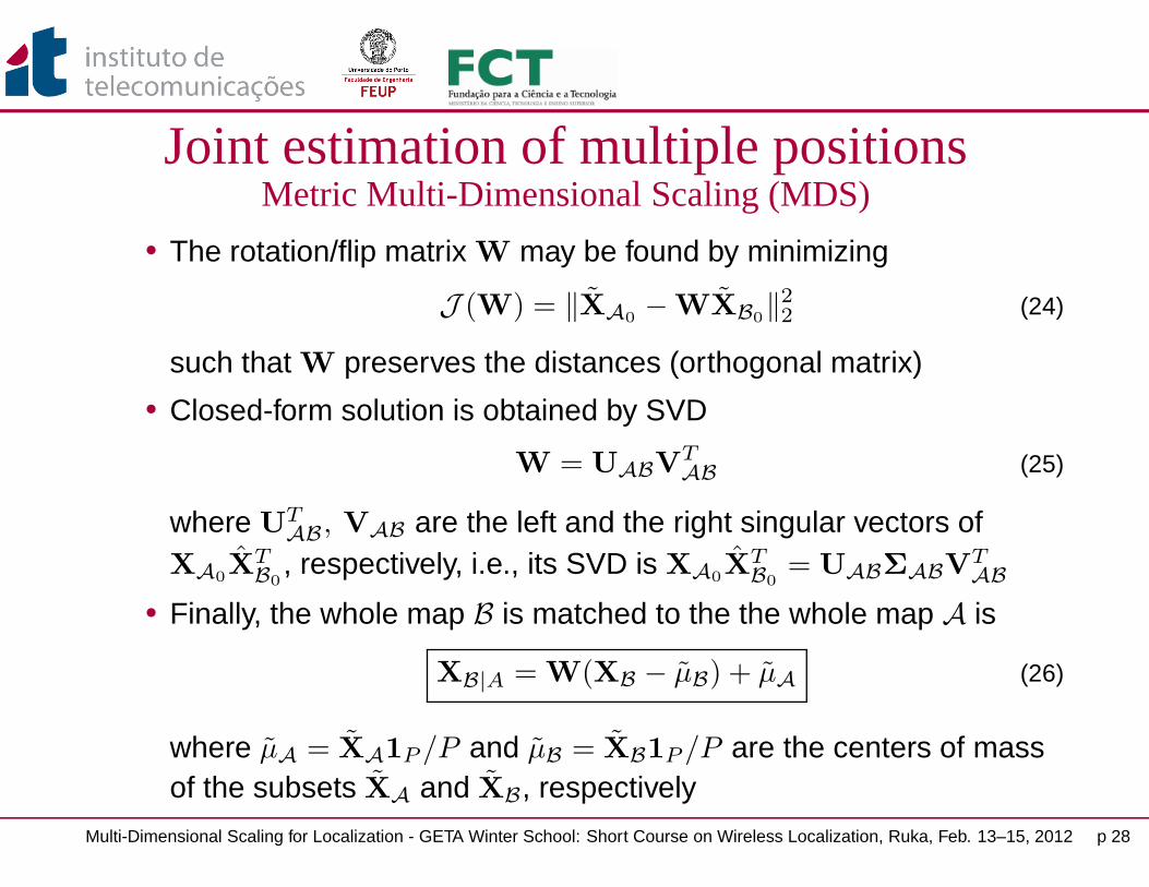
• The rotation/flip matrix W may be found by minimizing
J (W) = ‖XA0− WXB0
‖22 (24)
such that W preserves the distances (orthogonal matrix)• Closed-form solution is obtained by SVD
W = UABVTAB (25)
where UTAB, VAB are the left and the right singular vectors of
XA0X
TB0
, respectively, i.e., its SVD is XA0X
TB0
= UABΣABVTAB
• Finally, the whole map B is matched to the the whole map A is
XB|A = W(XB − µB) + µA (26)
where µA = XA1P /P and µB = XB1P /P are the centers of massof the subsets XA and XB, respectively
Multi-Dimensional Scaling for Localization - GETA Winter School: Short Course on Wireless Localization, Ruka, Feb. 13–15, 2012 p 28
Joint estimation of multiple positionsMetric Multi-Dimensional Scaling (MDS)
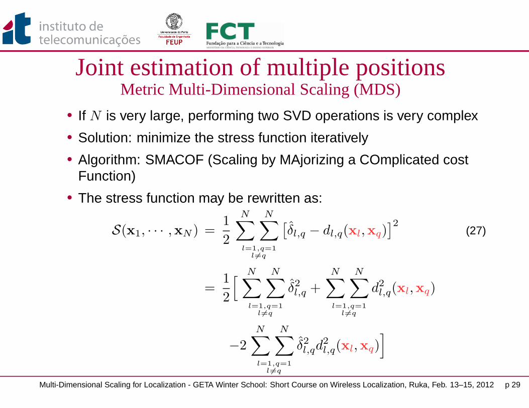
• If N is very large, performing two SVD operations is very complex• Solution: minimize the stress function iteratively• Algorithm: SMACOF (Scaling by MAjorizing a COmplicated cost
Function)• The stress function may be rewritten as:
S(x1, · · · ,xN ) =1
2
N∑
l=1,q=1
l6=q
N∑[δl,q − dl,q(xl,xq)
]2(27)
=1
2
[ N∑
l=1,q=1
l6=q
N∑δ2l,q +
N∑
l=1,q=1
l6=q
N∑d2
l,q(xl,xq)
−2N∑
l=1,q=1
l6=q
N∑δ2l,qd
2l,q(xl,xq)
]
Multi-Dimensional Scaling for Localization - GETA Winter School: Short Course on Wireless Localization, Ruka, Feb. 13–15, 2012 p 29

Joint estimation of multiple positionsMetric Multi-Dimensional Scaling (MDS)
• The stress function may be expressed in a convenient matrix form:
S(X) =1
2
N∑
l=1,q=1
l6=q
N∑δ2l,q − NtraceXHX
T − traceXΩ(X)XT (28)
where trace· denotes the trace operator (the sum of diagonalelements of a square matrix), and H is the centering matrix
• The matrix Ω depends on X, and its elements are of form
[Ω]l,q(X) = ωl,q(xl,xq) =
−δl,q
dl,q(xl,xq) , if l 6= q, dl,q(xl,xq) 6= 0
−∑N
p=1, p 6=l ωl,p(xl,xp), if l = q.(29)
• Due to Ω(X), the stress function (28) is not convex in X
Multi-Dimensional Scaling for Localization - GETA Winter School: Short Course on Wireless Localization, Ruka, Feb. 13–15, 2012 p 30
Joint estimation of multiple positionsMetric Multi-Dimensional Scaling (MDS)
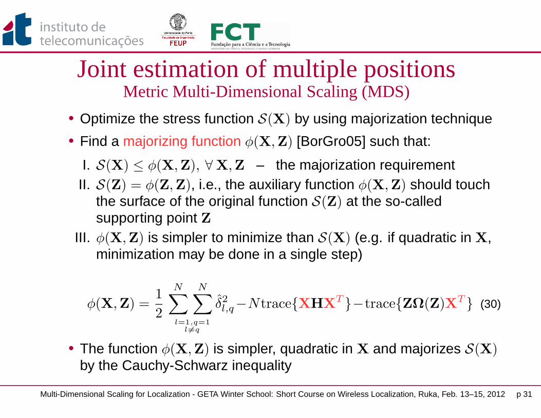
• Optimize the stress function S(X) by using majorization technique• Find a majorizing function φ(X,Z) [BorGro05] such that:
I. S(X) ≤ φ(X,Z), ∀ X,Z – the majorization requirementII. S(Z) = φ(Z,Z), i.e., the auxiliary function φ(X,Z) should touch
the surface of the original function S(Z) at the so-calledsupporting point Z
III. φ(X,Z) is simpler to minimize than S(X) (e.g. if quadratic in X,minimization may be done in a single step)
φ(X,Z) =1
2
N∑
l=1,q=1
l6=q
N∑δ2l,q−NtraceXHX
T −traceZΩ(Z)XT (30)
• The function φ(X,Z) is simpler, quadratic in X and majorizes S(X)by the Cauchy-Schwarz inequality
Multi-Dimensional Scaling for Localization - GETA Winter School: Short Course on Wireless Localization, Ruka, Feb. 13–15, 2012 p 31
Joint estimation of multiple positionsMetric Multi-Dimensional Scaling (MDS)
x
x0x1x2x∗
S(x)φ(x, x0)φ(x, x1)
S(x0) = φ(x0, x0)φ(x1, x0)
S(x1) = φ(x1, x1)φ(x2, x1)
S(x2)
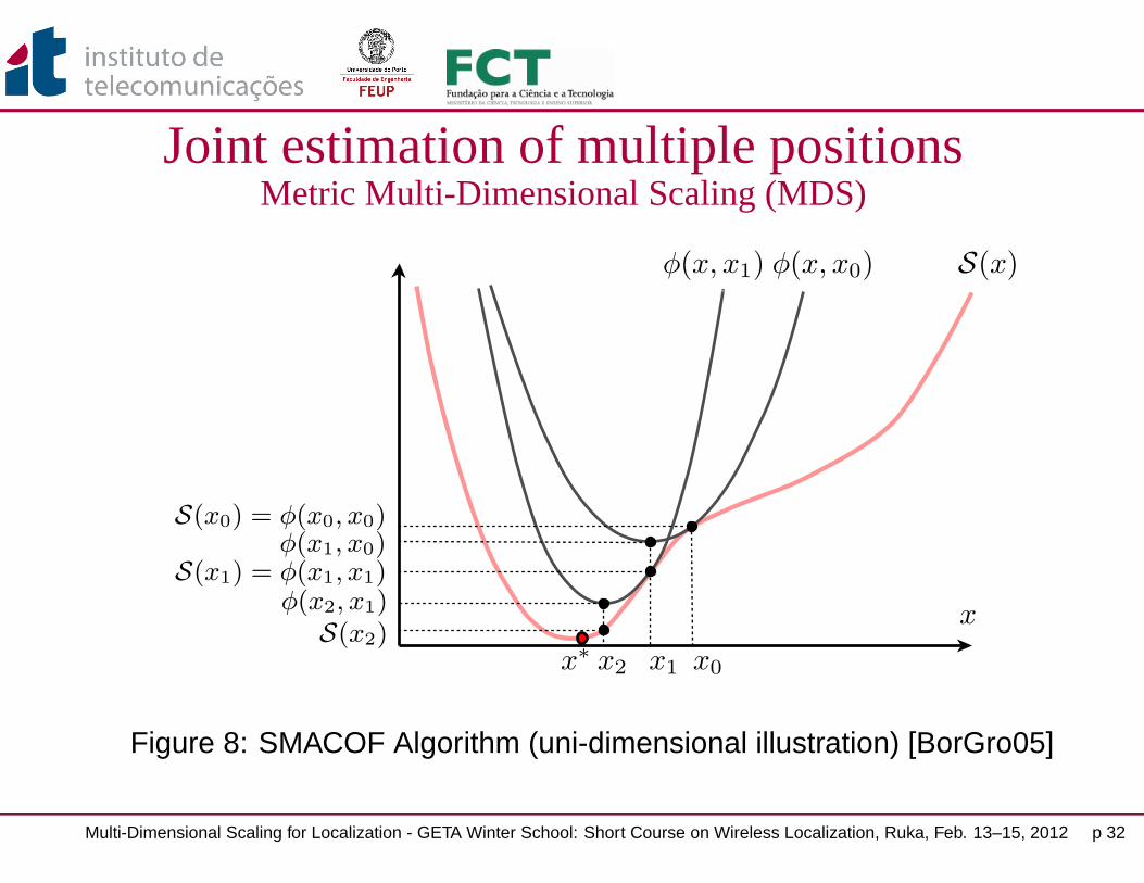
Figure 8: SMACOF Algorithm (uni-dimensional illustration) [BorGro05]
Multi-Dimensional Scaling for Localization - GETA Winter School: Short Course on Wireless Localization, Ruka, Feb. 13–15, 2012 p 32

Joint estimation of multiple positionsMetric Multi-Dimensional Scaling (MDS)
• SMACOF: Instead of optimizing the original function S(X), optimizethe auxiliary function φ(X,Z) – at every iteration k, take Z = Xk−1
• The gradient of φ(X,Z) w.r.t X is:
∇Xφ(X,Z) = NXH − ZΩ(Z) (31)
• Setting the gradient to zero, the closed-from minimum of φ(X,Z)w.r.t X for any Z is:
Xk =1
NZΩ(Z)H† (32)
• Considering the supporting point being the previous iterate, i.e.,Z = Xk−1,
Xk =1
NXk−1Ω(Xk−1)H
† (33)
• By the properties of H, we get the equivalent update
Xk = Xk−1 −1
N∇Xφ(Xk−1,Xk−1). (34)
Multi-Dimensional Scaling for Localization - GETA Winter School: Short Course on Wireless Localization, Ruka, Feb. 13–15, 2012 p 33
Joint estimation of multiple positionsMetric Multi-Dimensional Scaling (MDS)
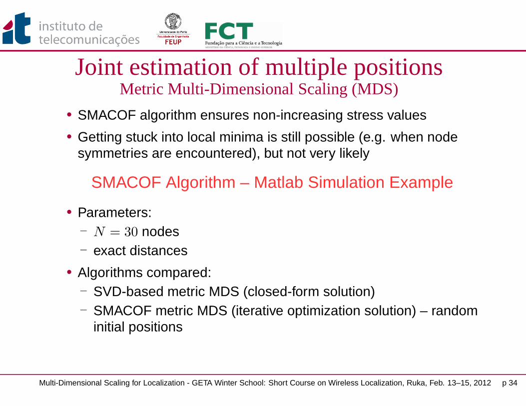
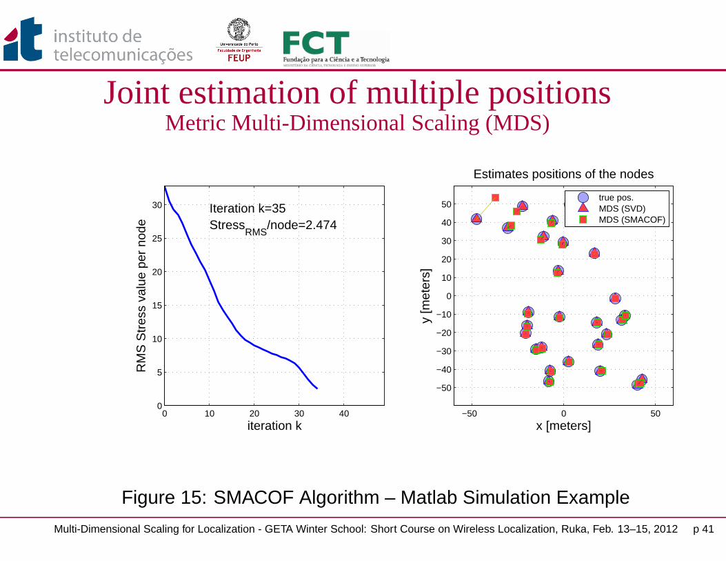
• SMACOF algorithm ensures non-increasing stress values• Getting stuck into local minima is still possible (e.g. when node
symmetries are encountered), but not very likely
SMACOF Algorithm – Matlab Simulation Example
• Parameters:− N = 30 nodes− exact distances
• Algorithms compared:− SVD-based metric MDS (closed-form solution)− SMACOF metric MDS (iterative optimization solution) – random
initial positions
Multi-Dimensional Scaling for Localization - GETA Winter School: Short Course on Wireless Localization, Ruka, Feb. 13–15, 2012 p 34

Joint estimation of multiple positionsMetric Multi-Dimensional Scaling (MDS)
0 10 20 30 400
5
10
15
20
25
30
StressRMS
/node=27.2626Iteration k=5
iteration k
RM
S S
tres
s va
lue
per
node
−50 0 50
−50
−40
−30
−20
−10
0
10
20
30
40
50
Estimates positions of the nodes
x [meters]y
[met
ers]
true pos.MDS (SVD)MDS (SMACOF)
Figure 9: SMACOF Algorithm – Matlab Simulation Example
Multi-Dimensional Scaling for Localization - GETA Winter School: Short Course on Wireless Localization, Ruka, Feb. 13–15, 2012 p 35
Joint estimation of multiple positionsMetric Multi-Dimensional Scaling (MDS)
0 10 20 30 400
5
10
15
20
25
30
StressRMS
/node=20.2153Iteration k=10
iteration k
RM
S S
tres
s va
lue
per
node
−50 0 50
−50
−40
−30
−20
−10
0
10
20
30
40
50
Estimates positions of the nodes
x [meters]y
[met
ers]
true pos.MDS (SVD)MDS (SMACOF)
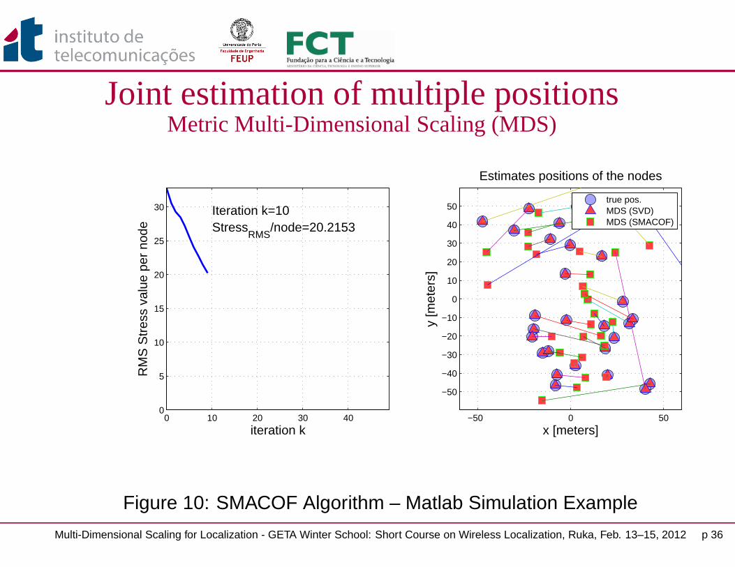
Figure 10: SMACOF Algorithm – Matlab Simulation Example
Multi-Dimensional Scaling for Localization - GETA Winter School: Short Course on Wireless Localization, Ruka, Feb. 13–15, 2012 p 36

Joint estimation of multiple positionsMetric Multi-Dimensional Scaling (MDS)
0 10 20 30 400
5
10
15
20
25
30
StressRMS
/node=13.298Iteration k=15
iteration k
RM
S S
tres
s va
lue
per
node
−50 0 50
−50
−40
−30
−20
−10
0
10
20
30
40
50
Estimates positions of the nodes
x [meters]y
[met
ers]
true pos.MDS (SVD)MDS (SMACOF)
Figure 11: SMACOF Algorithm – Matlab Simulation Example
Multi-Dimensional Scaling for Localization - GETA Winter School: Short Course on Wireless Localization, Ruka, Feb. 13–15, 2012 p 37
Joint estimation of multiple positionsMetric Multi-Dimensional Scaling (MDS)
0 10 20 30 400
5
10
15
20
25
30
StressRMS
/node=9.4173Iteration k=20
iteration k
RM
S S
tres
s va
lue
per
node
−50 0 50
−50
−40
−30
−20
−10
0
10
20
30
40
50
Estimates positions of the nodes
x [meters]y
[met
ers]
true pos.MDS (SVD)MDS (SMACOF)
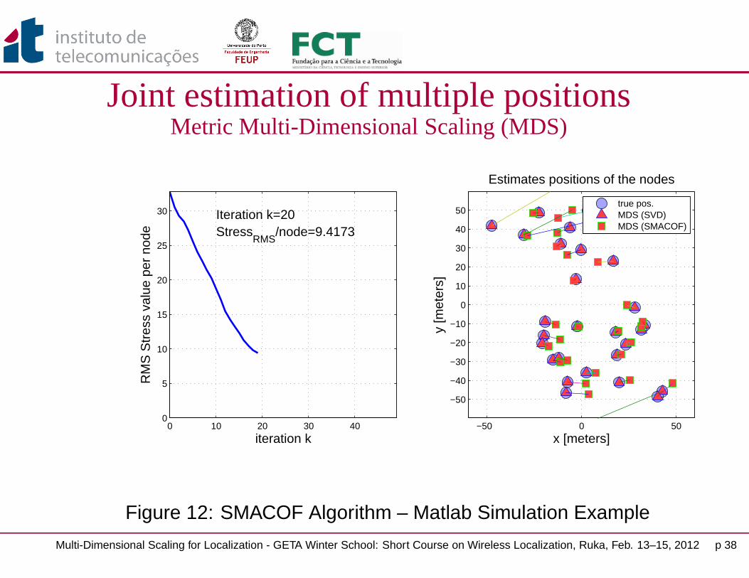
Figure 12: SMACOF Algorithm – Matlab Simulation Example
Multi-Dimensional Scaling for Localization - GETA Winter School: Short Course on Wireless Localization, Ruka, Feb. 13–15, 2012 p 38

Joint estimation of multiple positionsMetric Multi-Dimensional Scaling (MDS)
0 10 20 30 400
5
10
15
20
25
30
StressRMS
/node=7.8043Iteration k=25
iteration k
RM
S S
tres
s va
lue
per
node
−50 0 50
−50
−40
−30
−20
−10
0
10
20
30
40
50
Estimates positions of the nodes
x [meters]y
[met
ers]
true pos.MDS (SVD)MDS (SMACOF)
Figure 13: SMACOF Algorithm – Matlab Simulation Example
Multi-Dimensional Scaling for Localization - GETA Winter School: Short Course on Wireless Localization, Ruka, Feb. 13–15, 2012 p 39
Joint estimation of multiple positionsMetric Multi-Dimensional Scaling (MDS)
0 10 20 30 400
5
10
15
20
25
30
StressRMS
/node=6.3371Iteration k=30
iteration k
RM
S S
tres
s va
lue
per
node
−50 0 50
−50
−40
−30
−20
−10
0
10
20
30
40
50
Estimates positions of the nodes
x [meters]y
[met
ers]
true pos.MDS (SVD)MDS (SMACOF)
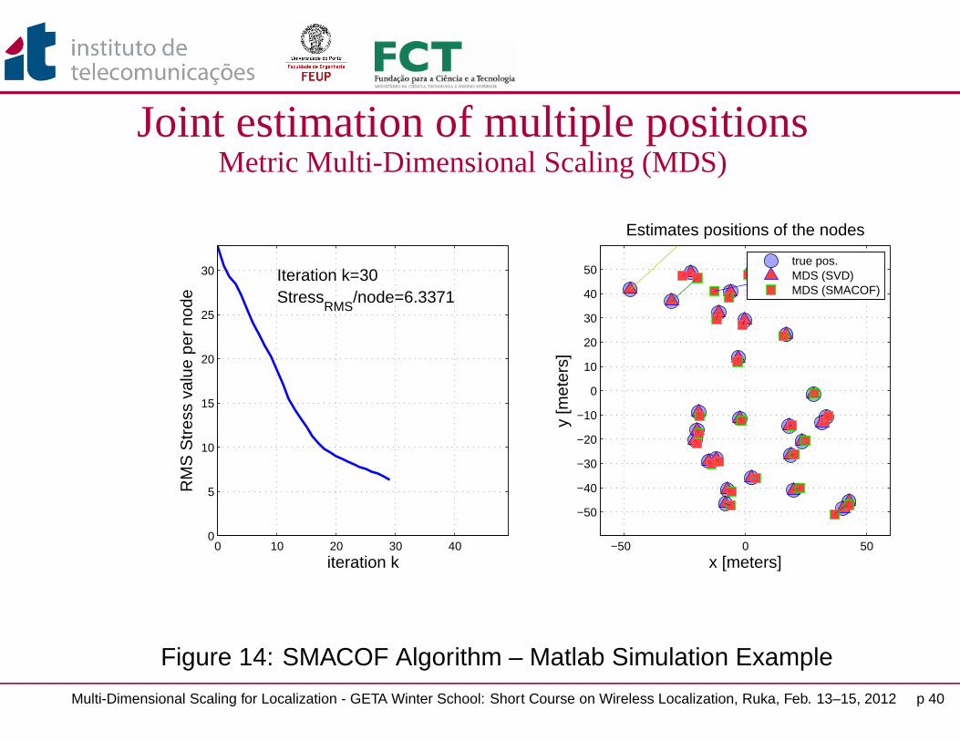
Figure 14: SMACOF Algorithm – Matlab Simulation Example
Multi-Dimensional Scaling for Localization - GETA Winter School: Short Course on Wireless Localization, Ruka, Feb. 13–15, 2012 p 40
Joint estimation of multiple positionsMetric Multi-Dimensional Scaling (MDS)
0 10 20 30 400
5
10
15
20
25
30
StressRMS
/node=2.474Iteration k=35
iteration k
RM
S S
tres
s va
lue
per
node
−50 0 50
−50
−40
−30
−20
−10
0
10
20
30
40
50
Estimates positions of the nodes
x [meters]y
[met
ers]
true pos.MDS (SVD)MDS (SMACOF)
Figure 15: SMACOF Algorithm – Matlab Simulation Example
Multi-Dimensional Scaling for Localization - GETA Winter School: Short Course on Wireless Localization, Ruka, Feb. 13–15, 2012 p 41

Joint estimation of multiple positionsMetric Multi-Dimensional Scaling (MDS)
0 10 20 30 400
5
10
15
20
25
30
StressRMS
/node=0.81537Iteration k=40
iteration k
RM
S S
tres
s va
lue
per
node
−50 0 50
−50
−40
−30
−20
−10
0
10
20
30
40
50
Estimates positions of the nodes
x [meters]y
[met
ers]
true pos.MDS (SVD)MDS (SMACOF)
Figure 16: SMACOF Algorithm – Matlab Simulation Example
Multi-Dimensional Scaling for Localization - GETA Winter School: Short Course on Wireless Localization, Ruka, Feb. 13–15, 2012 p 42

Joint estimation of multiple positionsMetric Multi-Dimensional Scaling (MDS)
0 10 20 30 400
5
10
15
20
25
30
StressRMS
/node=0.28418Iteration k=45
iteration k
RM
S S
tres
s va
lue
per
node
−50 0 50
−50
−40
−30
−20
−10
0
10
20
30
40
50
Estimates positions of the nodes
x [meters]y
[met
ers]
true pos.MDS (SVD)MDS (SMACOF)
Figure 17: SMACOF Algorithm – Matlab Simulation Example
Multi-Dimensional Scaling for Localization - GETA Winter School: Short Course on Wireless Localization, Ruka, Feb. 13–15, 2012 p 43

Joint estimation of multiple positionsMetric Multi-Dimensional Scaling (MDS)
0 10 20 30 400
5
10
15
20
25
30
StressRMS
/node=0.10031Iteration k=50
iteration k
RM
S S
tres
s va
lue
per
node
−50 0 50
−50
−40
−30
−20
−10
0
10
20
30
40
50
Estimates positions of the nodes
x [meters]y
[met
ers]
true pos.MDS (SVD)MDS (SMACOF)
Figure 18: SMACOF Algorithm – Matlab Simulation Example
Multi-Dimensional Scaling for Localization - GETA Winter School: Short Course on Wireless Localization, Ruka, Feb. 13–15, 2012 p 44

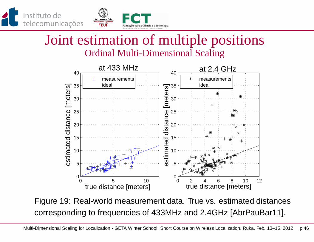
Joint estimation of multiple positionsOrdinal Multi-Dimensional Scaling
• In practice, range estimation is subject to very large errors• Preserving the exact distances is not possible (e.g. incompatible
set of distances)• Therefore, the metric assumption becomes unnecessary• Different transformations of the distance may be used
• Estimated distances δp,q are replaced by pseudo-distances f(δp,q)
• Ordinal MDS (OMDS): Instead of attempting to preserve the exactdistances between nodes, try to preserve only their ordering
• Use a monotonically increasing distance mapping function f (calledpseudo-distance or disparity) – f can be determined experimentally(e.g. by using isotonic regression, monotone splines, etc.)
• It achieves better performance than the metric MDS (and lowerstress values) [AbrPauBar11, ZhoLawChi10, VivWon06]
Multi-Dimensional Scaling for Localization - GETA Winter School: Short Course on Wireless Localization, Ruka, Feb. 13–15, 2012 p 45
Joint estimation of multiple positionsOrdinal Multi-Dimensional Scaling
0 5 100
5
10
15
20
25
30
35
40
true distance [meters]
estim
ated
dis
tanc
e [m
eter
s]at 433 MHz
measurementsideal
0 2 4 6 8 10 120
5
10
15
20
25
30
35
40
true distance [meters]
estim
ated
dis
tanc
e [m
eter
s]
at 2.4 GHz
measurementsideal
Figure 19: Real-world measurement data. True vs. estimated distancescorresponding to frequencies of 433MHz and 2.4GHz [AbrPauBar11].
Multi-Dimensional Scaling for Localization - GETA Winter School: Short Course on Wireless Localization, Ruka, Feb. 13–15, 2012 p 46

Joint estimation of multiple positionsOrdinal Multi-Dimensional Scaling
Transformation disparity function f(δp,q)
Absolute δp,q
Ratio cδp,q with c > 0
Interval a + bδp,q with a ≥ 0, b ≥ 0
Spline A sum of monotone polynomials of δp,q
Ordinal Preserve the original order of δp,q
Table 1: Some MDS models ordered by the scale level of the proximities(from strong to weak) [BorGro05].
• Non-metric MDS: order matters just qualitatively, not quantitatively• No strict montonicity requirement – no mapping needs to be
specified
Multi-Dimensional Scaling for Localization - GETA Winter School: Short Course on Wireless Localization, Ruka, Feb. 13–15, 2012 p 47

Joint estimation of multiple positionsWeighted Multi-Dimensional Scaling (wMDS)
• If reliability information is available – weighted approach[CosPatHer06]
Weighted MDS• accuracies rn are assigned to each node n’s position• Nodes are classified as follows:
− A anchor nodes – perfect knowledge of their location rn = 1− B unknown location nodes – imperfect or no a priori position
information 0 ≤ rn < 1− the total number of nodes is N = A + B
• Generalization: consider that J estimates δjl,q, j = 1, . . . , J are
available for each distance dl,q
Multi-Dimensional Scaling for Localization - GETA Winter School: Short Course on Wireless Localization, Ruka, Feb. 13–15, 2012 p 48

Joint estimation of multiple positionsWeighted Multi-Dimensional Scaling (wMDS)
• The weighted Stress function is
S(x1, · · · ,xB) =B∑
b=1
N∑
n 6=b
n=1
J∑
j=l
wb,n
[δkb,n−db,n(xb,xn)
]2+
B∑
b=1
rb‖xb−xb‖22
(35)where the weights wb,n can be selected to predict the accuracy ofthe measurement δb,n
• if no such information is available, then wb,n = 1
• the weights are symmetric wb,n = wn,b and wn,n = 0
• the vector xb contains prior knowledge about locations• reliability rb determines the influence of such knowledge on S
• No closed-form solution to the wMDS problem exists – use theSMACOF iterative approach [BorGro05]
Multi-Dimensional Scaling for Localization - GETA Winter School: Short Course on Wireless Localization, Ruka, Feb. 13–15, 2012 p 49

Joint estimation of multiple positionsWeighted Multi-Dimensional Scaling (wMDS)
• In WSN, nodes possess low amount of energy, modestcomputational capabilities and low bandwidth
• Centralized MDS requires communicating all information to a fusioncenter− gather all the pairwise range measurements from each sensor
and reliability information− perform centralized map construction− send back the coordinates of each device
• This is feasible when the number of nodes is low
Multi-Dimensional Scaling for Localization - GETA Winter School: Short Course on Wireless Localization, Ruka, Feb. 13–15, 2012 p 50
Cooperative localizationDistributed Weighted Multi-Dimensional Scaling (dwMDS)
• Number of network nodes N may be very large• Centralized localization is not feasible – scalability issues• The protocol for communicating location-related data across the
network becomes crucial• Critical aspects:
− Bandwidth (huge amount of information to the fusion center)− Delay (perishable information) – less critical in some
applications, depending on the update rate
Multi-Dimensional Scaling for Localization - GETA Winter School: Short Course on Wireless Localization, Ruka, Feb. 13–15, 2012 p 51
Cooperative localizationDistributed Weighted Multi-Dimensional Scaling (dwMDS)• Goal: Distributed localization schemes – no fusion center available
[PatAshKyp05]− limit the communications costs (usually higher than the
computational costs)− the computational costs are shared among nodes− when a node moves w.r.t. the others - local position is more
relevant• The total stress function S may be written as a sum of local stress
functions Sb
S(x1, . . . ,xB) =B∑
b=1
Sb(x1, . . . ,xB) (36)
• A local stress function at each node b is minimized instead• Local stress minimization results into global stress minimization
Multi-Dimensional Scaling for Localization - GETA Winter School: Short Course on Wireless Localization, Ruka, Feb. 13–15, 2012 p 52
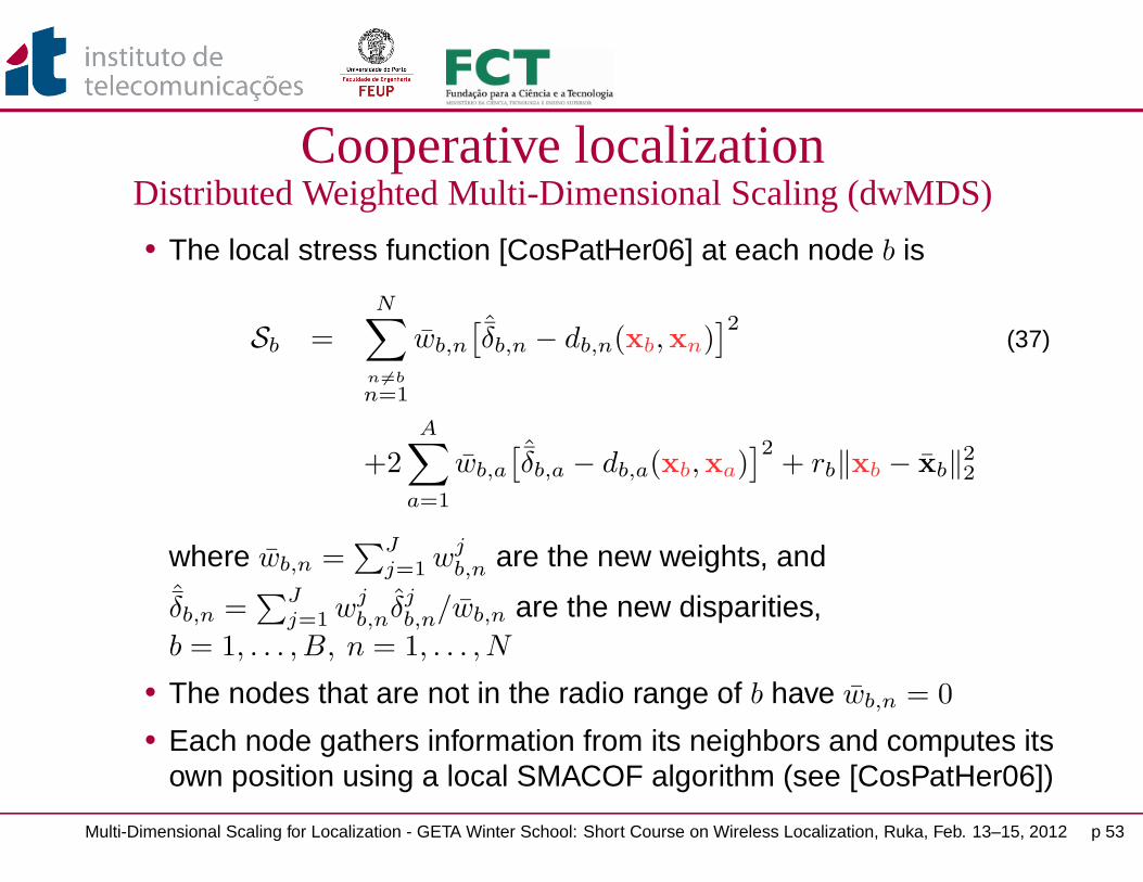
Cooperative localizationDistributed Weighted Multi-Dimensional Scaling (dwMDS)• The local stress function [CosPatHer06] at each node b is
Sb =N∑
n 6=b
n=1
wb,n
[ˆδb,n − db,n(xb,xn)]2
(37)
+2A∑
a=1
wb,a
[ˆδb,a − db,a(xb,xa)]2
+ rb‖xb − xb‖22
where wb,n =∑J
j=1 wjb,n are the new weights, and
ˆδb,n =∑J
j=1 wjb,nδj
b,n/wb,n are the new disparities,b = 1, . . . , B, n = 1, . . . , N
• The nodes that are not in the radio range of b have wb,n = 0
• Each node gathers information from its neighbors and computes itsown position using a local SMACOF algorithm (see [CosPatHer06])
Multi-Dimensional Scaling for Localization - GETA Winter School: Short Course on Wireless Localization, Ruka, Feb. 13–15, 2012 p 53

Cooperative localizationDistributed Weighted Multi-Dimensional Scaling (dwMDS)
reference nodes unknown nodes
Figure 20: Cooperative localization – neighbors help locate each other
Multi-Dimensional Scaling for Localization - GETA Winter School: Short Course on Wireless Localization, Ruka, Feb. 13–15, 2012 p 54
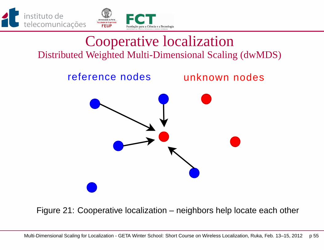
Cooperative localizationDistributed Weighted Multi-Dimensional Scaling (dwMDS)
reference nodes unknown nodes
Figure 21: Cooperative localization – neighbors help locate each other
Multi-Dimensional Scaling for Localization - GETA Winter School: Short Course on Wireless Localization, Ruka, Feb. 13–15, 2012 p 55

Cooperative localizationDistributed Weighted Multi-Dimensional Scaling (dwMDS)
reference nodes unknown nodes
Figure 22: Cooperative localization – neighbors help locate each other
Multi-Dimensional Scaling for Localization - GETA Winter School: Short Course on Wireless Localization, Ruka, Feb. 13–15, 2012 p 56

MDSThe problem of missing distances
• Several approaches exist in the literature− map stitching – previously presented (see also [KwoSon08] and
MDS-MAP(P) [ShaRumZha04])− split the network in connected and disconnected parts
[AmaWanLeu10]− distance matrix completion – the “missing data” problem
Shortest path algorithm MDS-MAP(C) [ShaRumZha04]Algebraic approaches: e.g. SVD approach [DriIsmPan06]
− Distributed algorithms do not face the “missing distance” problem
Multi-Dimensional Scaling for Localization - GETA Winter School: Short Course on Wireless Localization, Ruka, Feb. 13–15, 2012 p 57

Extensions of MDS• MDS has been extended to TDoA as well (see e.g. [ZhoLawChi10]
and references therein)• Modified MDS that include angle information exist
− Modified stress function (highly non-linear) [EliHaz10] –minimized by using Levenberg-Marquardt algorithm
Sα(x1, · · · ,xN ) =N∑
l=1,q=1
l6=q
N∑ [δl,q − dl,q(xl,xq)
]2
+N∑
l=1,q=1
l6=q
N∑arctan
yl − yq
xl − xq− αl,q (38)
− Super-MDS [AbrDes07]: graph-theoretical approach – edges asvectors vl,q – distance matrix is replaced by a matrix whoseentries are scalar products of form 〈vl,p,vp,q〉 = dl,pdp,q cos αl,q
Multi-Dimensional Scaling for Localization - GETA Winter School: Short Course on Wireless Localization, Ruka, Feb. 13–15, 2012 p 58

Extensions of MDS• Other MDS approaches exist
− Squared distances matrix is replaced by other matrices:distances (not squared) or coordinates
− The range errors has a very different impact on the algorithmperformance (multiplicative vs. additive noise)
− Each approach has its own type of solution (in general, asubspace solution, e.g., matrix decompositions, projections, etc.)
• Various statistical analyses assuming different error distributionsare also available (sensitivity, CRLB, MSE, etc.)
• More details on the existing literature and algorithmsimplementation – available upon request to [email protected]
Multi-Dimensional Scaling for Localization - GETA Winter School: Short Course on Wireless Localization, Ruka, Feb. 13–15, 2012 p 59

Recent Work• Joint work with L. M. Paula, J. Barros, J. P. S. Cunha, and N. B.
Carvalho [AbrPauBar11]• This work was supported by:
− FCT (Fundação para a Ciência e a Tecnologia) through the VR(Vital Responder) project (within the Carnegie-Mellon|Portugalprogram. ref. CMU-P/CPS/0046/2008),
− CALLAS (Calculi and Languages for Sensor Networks) project(ref. PTDC/EIA/71462/2006)
− FEDER (Fundo Europeu de Desenvolvimento Regional).
Multi-Dimensional Scaling for Localization - GETA Winter School: Short Course on Wireless Localization, Ruka, Feb. 13–15, 2012 p 60

Recent Work• We proposed a dual frequency approach for WSN localization• The sensor nodes are equipped with two RF front-ends operating
at 433MHz and 2.4GHz, respectively• The propagation at the two frequencies differs substantially• Frequency diversity is exploited• Algorithm:
− Ranging: RSSI, channel models at the two frequencies− Position estimation: ordinal multi-dimensional scaling− Position tracking: Kalman filter + simple motion model
• We use real-world measurements to assess the systemperformance
Multi-Dimensional Scaling for Localization - GETA Winter School: Short Course on Wireless Localization, Ruka, Feb. 13–15, 2012 p 61
Real-world Results
A1 A2
A3A4 starting point
18
18
ending point
25
West−East axis [meters]
Sou
th−
Nor
th a
xis
[met
ers]
Indoor location estimation and tracking
0 2 4 6 8 10
0
1
2
3
4
5
6
7
8
9
10 anchor nodestrue pos.est. pos. (MLT)est. pos. (OMDS)tracked pos. (KF)
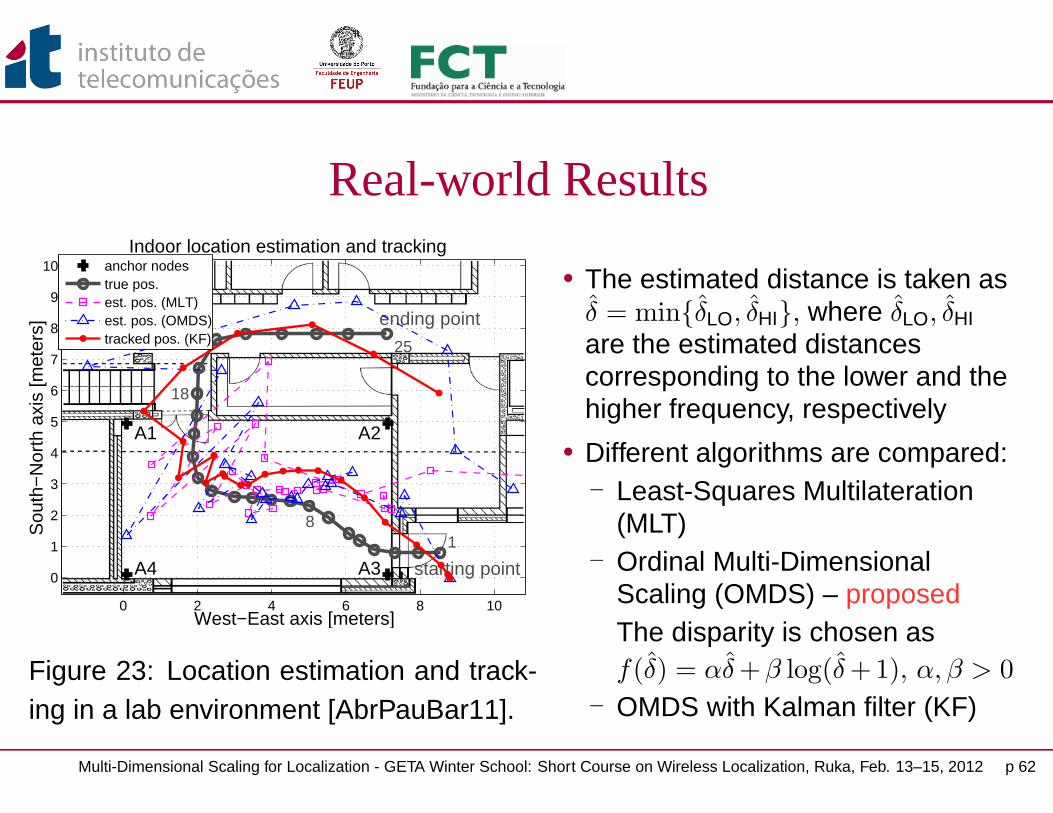
Figure 23: Location estimation and track-ing in a lab environment [AbrPauBar11].
• The estimated distance is taken asδ = minδLO, δHI, where δLO, δHI
are the estimated distancescorresponding to the lower and thehigher frequency, respectively
• Different algorithms are compared:− Least-Squares Multilateration
(MLT)− Ordinal Multi-Dimensional
Scaling (OMDS) – proposedThe disparity is chosen asf(δ) = αδ +β log(δ +1), α, β > 0
− OMDS with Kalman filter (KF)
Multi-Dimensional Scaling for Localization - GETA Winter School: Short Course on Wireless Localization, Ruka, Feb. 13–15, 2012 p 62
Conclusions• Multi-Dimensional Scaling proved to be a powerful tool for
estimating the locations of multiple nodes
• It is suitable for both relative positioning and absolute positioning(that requires anchor nodes)
• Different MDS versions are available, with various degrees ofaccuracy and complexity
• The choice strongly depends upon the practical application at hand
• The most common technical limitations include: energy, bandwidth,computational power and sensing capabilities
Multi-Dimensional Scaling for Localization - GETA Winter School: Short Course on Wireless Localization, Ruka, Feb. 13–15, 2012 p 63

References[AbrPauBar11] T. E. Abrudan, L. M. Paula, J. Barros, J. P. S. Cunha, and N. B. Carvalho, “Indoor Location
Estimation and Tracking in Wireless Sensor Networks using a Dual Frequency Approach”, 2011IEEE International Conference on Indoor Positioning and Indoor Navigation (IPIN), Guimarães,Portugal, 21–23 Sep. 2011.
[HagAbrKoi09] A. Haghparast, T. Abrudan and V. Koivunen, “OFDM ranging in multipath channels usingtime-reversal method”, 10th IEEE International Workshop on Signal Processing Advances forWireless Communications (SPAWC ’09), pp. 568–572, 21–24 Jun. 2009.
[AbrHagKoi12] T. Abrudan , A. Haghparast and V. Koivunen, “Time-Synchronization and Ranging for OFDMSystems Using Time-Reversal Technique”, to be submitted (2012).
[SayTarKha05] A. H. Sayed, A. Tarighat, N. Khajehnouri, “Network-based wireless location”, IEEE SignalProcessing Magazine, pp. 24–40, July 2005.
[BorGro05] I. Borg, P. Groenen, “Modern Multidimensional Scaling” Springer, 2005.
[CosPatHer06] J. A. Costa, N. Patwari, A. O Hero III “Distributed Weighted-Multidimensional Scaling”, ACMTransactions on Sensor Networks, vol. 2, no. 1, pp. 39–64 Feb. 2006.
[PatAshKyp05] N. Patwari, J. N. Ash, S. Kyperountas, A. O. Hero III, R. L. Moses, N. S. Correal, “Locating thenodes: cooperative localization in wireless sensor networks”, IEEE Signal Processing Magazine,vol.22, no.4, pp. 54–69, Jul. 2005.
Multi-Dimensional Scaling for Localization - GETA Winter School: Short Course on Wireless Localization, Ruka, Feb. 13–15, 2012 p 64
References[KwoSon08] O.-H. Kwon, H.-J. Song, “Localization through Map Stitching in Wireless Sensor Networks”,
IEEE Transactions on Parallel and Distributed computing, vol. 19, no. 1, pp. 93–105, Jan. 2008.
[ShaRumZha04] Y. Shang, W. Ruml, Y. Zhang, M. Fromherz, “Localization from connectivity in sensor networks,”IEEE Transactions on Parallel and Distributed Systems, vol.15, no.11, pp. 961–974, Nov. 2004.
[AmaWanLeu10] A. Amar and Yiyin Wang and G. Leus, “Extending the Classical Multidimensional ScalingAlgorithm Given Partial Pairwise Distance Measurements”, IEEE Signal Processing Letters, vol.17, no. 5, pp. 473–476, May 2010.
[DriIsmPan06] P. Drineas, M. Magdon-Ismail, G. Pandurangan, R. Virrankoski and A. Savvides, “Distancematrix reconstruction from incomplete distance information for sensor network localization”, inProc. IEEE SECON 2006, pp. 536–544, 2006.
[ZhoLawChi10] Y. Zhou, C. L. Law, and F. Chin, “Construction of Local Anchor Map for Indoor PositionMeasurement System”, IEEE Transactions on Instrumentation and Measurement, vol. 59, no. 7,pp. 1986–1988, 2010.
[VivWon06] V. Vivekanandan, and V.W.S. Wong, “Ordinal MDS-Based Localization for Wireless SensorNetworks”, IEEE 64th Vehicular Technology Conference, VTC-2006 Fall, pp. 1–5, 25-28 Sept.2006.
Multi-Dimensional Scaling for Localization - GETA Winter School: Short Course on Wireless Localization, Ruka, Feb. 13–15, 2012 p 65
References[CheWeiWan09] Zhang-Xin Chen; He-Wen Wei; Qun Wan; Shang-Fu Ye; Wan-Lin Yang, “A Supplement to
Multidimensional Scaling Framework for Mobile Location: A Unified View”, IEEE Transactions onSignal Processing, vol. 57, no. 5, pp. 2030–2034, May 2009.
[EllHaz10] C. Ellis and M. Hazas “A comparison of MDS-MAP and non-linear regression” 2011 IEEEInternational Conference on Indoor Positioning and Indoor Navigation (IPIN), Guimarães,Portugal, 21–23 Sep. 2011.
[AbrDes07] G.T. Freitas de Abreu, G. Destino, “Super MDS: Source Location from Distance and AngleInformation”, IEEE Wireless Communications and Networking Conference, WCNC 2007,pp.4430–4434, 11-15 March 2007.
[Lee05] Duke Lee, “Localization using Multidimensional Scaling (LMDS)”, PhD. Thesis, University ofCalifornia, Berkeley, 2005.
Multi-Dimensional Scaling for Localization - GETA Winter School: Short Course on Wireless Localization, Ruka, Feb. 13–15, 2012 p 66