Multi-dimensional homoclinic jumpingand the discretized NLS equation�G. HALLERyDivision of Applied Mathematics, Box FBrown University, Providence, RI 02912Email: haller@cfm.brown.eduAbstractWe consider a class of dynamical systems that arise frequently in multi-mode truncationsand discretizations of partial di�erential equations, including the perturbed NLS. We developa general method to detect the existence of multi-pulse solutions that are doubly asymptoticto an invariant manifold with two di�erent time scales. We use our method together withsome recent results of Li and McLaughlin to show the existence of several families of multi-pulse orbits for the Ablowitz-Ladik discretization of the perturbed NLS. These orbits includeN -pulse heteroclinic orbits and N -pulse �Silnikov-type orbits for arbitrarily large N .Running title: Multi-pulse homoclinic orbits1 IntroductionIn this paper we study a class of multi-degree-of-freedom dynamical systems which arise in modaltruncations of partial di�erential equations on periodic domains. One usually arrives at theseequations when looking for small amplitude solutions of a PDE with parametric forcing terms.An important prototype example is the damped-forced sine-Gordon equation, which we discussbrie y below for motivation.As shown in, e.g., Bishop et al. [5], a small amplitude approximation to the sine-Gordonequation leads to a perturbed nonlinear Schr�odinger equation (NLS). For a range of parameters,the integrable limit of the NLS admits one linearly stable and one unstable mode together within�nitely many neutrally stable modes. These latter modes can be further decomposed into amode of plane waves (i.e., solutions with no spatial structure) and an in�nite number of neutrallystable, i.e., oscillatory modes. A �nite dimensional approximation to the problem is a well-known discretization of the NLS that produces an integrable system in the unperturbed limit(see Ablowitz and Ladik [1], Bogolyubov and Prikarpatskii [7], and Miller et al. [36]).In the discretized NLS the plane of spatially independent solutions is invariant under both theperturbed and the unperturbed dynamics. For zero dissipation and forcing, the plane containsa circle of �xed points which is surrounded by a one-parameter family of periodic solutions.Furthermore, the invariant plane lies in a codimension two center manifold that accounts forthe non-planar oscillatory modes. The center manifold is normally hyperbolic as it admits aone-dimensional stable and a one-dimensional unstable subspace at each of its points. Thishyperbolicity is due to the presence of the stable and unstable modes mentioned above, and gives�Submitted to Comm. Math. PhysyPartially supported by NSF Grant DMS-95011239 and AFOSR Grant F49620-95-1-00851

rise to codimension one stable and unstable manifolds to the center manifold. These invariantmanifolds then coincide in two homoclinic manifolds in the integrable limit of zero forcing anddamping. This phase space geometry is quite remarkable as it is a precise �nite dimensionalmodel of the phase space structure of the original PDE (see, e.g., Ercolani et al. [8], Ercolaniand McLaughlin [9], and Li and McLaughlin [30] for details).A similar analogy exists between the phase space structure of the perturbed NLS equationand its two-mode approximation (see Bishop et al. [5], [6]). This fact inspired a great deal ofwork on modal truncations of the perturbed NLS, although all rigorous results so far are onlyconcerned with the two-mode approximation that excludes the oscillatory modes (see Bishopet al. [5], [6], Kova�ci�c and Wiggins [27], Haller and Wiggins [16], McLaughlin et al. [34], andHaller and Wiggins [19]). Other examples with the modal truncations of the same class includeparametrically forced surface wave problems (Holmes [22], and Kambe and Umeki [25]), thedynamics of forced and damped thin plates (Feng and Sethna [10]), inextensional beams (Nayfehand Pai [37], Feng and Leal [12]), and resonantly driven coupled pendula (Miles [35], Becker andMiles [4], and Kova�ci�c and Wettergren [28]). All these problems can be recast in the form ofequation (1) below. Our basic goal in this paper is to study the existence of nontrivial homoclinicand heteroclinic behavior in these systems by including an arbitrary high but �nite number ofmodes.The main result of the paper is the construction of a class of complicated solutions in multi-mode truncations or discretizations. These solutions admit three di�erent time scales and corre-spond to irregular \jumping" around the plane � of spatially independent modes. In our generalformulation we in fact allow for the presence of a 2m-dimensional manifold � which contains anm-torus of equilibria in the unperturbed limit.In backward time the solutions we construct asymptote to some set in � which is born outof the perturbation of the torus of �xed points of the unperturbed limit. In forward time, aftermaking several jumps away from �, the solutions asymptote to other structures in the centermanifold that lie in the vicinity of the manifold �: We give a criterion for the existence of suchsolutions, which is a generalization of the energy-phase method developed in Haller [15] and Hallerand Wiggins [19] for two-degree-of-freedom systems.Under certain conditions, the solutions we construct will ultimately asymptote to some invari-ant set within the manifold �. If their ! and �-limit sets coincide, then we obtain a multi-pulseorbit homoclinic to this set. An important special case arises when this set is an equilibriumthat is a sink for the dynamics on the codimension two center manifold. We call the resultingmulti-pulse orbit an N -pulse �Silnikov-type orbit. Such orbits seem to have a prominent role increating complicated or chaotic dynamics in modal equations. While single-pulse �Silnikov or-bits can also be obtained in these problems applying a modi�ed Melnikov method (see Kova�ci�cand Wiggins [27], Feng and Sethna [10], Feng and Wiggins [11], Tien and Namachchivaya [38],Kova�ci�c and Wettergren [28]), and Li and McLaughlin [31], such orbits generically exist for asingle codimension one surface in the space of system parameters. In contrast, our methodstypically yield multi-pulse �Silnikov-type orbits on an intricate web of the parameter space (seeHaller and Wiggins [19] for a two-mode example).The main techniques we use in this paper include the perturbation theory of normally hyper-bolic invariant manifolds, their stable and unstable manifolds, and stable and unstable foliations.We do not explicitly assume that in the limit of zero forcing and damping the modal equationsare integrable. We do, however, assume the presence of particular structures in this limitinggeometry, which are not typical in nonintegrable cases. Our strategy is to follow trajectories inthe unstable manifold of the manifold � as they leave and repeatedly return to a neighborhood ofthe center manifold. The control over individual trajectories is achieved by obtaining estimateson their location as well as on their energies before and after their intermediate passages near2

the center manifold. This amounts to studying the properties of an appropriately de�ned localPoincar�e map. The results of this study are summarized in the Passage Lemma (Lemma 7.1),which sets the stage for a �nal implicit function argument in Theorem 7.3 of section 6. This ar-gument is subtle since the equation satis�ed by multi-pulse homoclinic orbits becomes unde�nedin the limit of the vanishing perturbation parameter. We circumvent this problem by de�ningan extension to the local map at this limit, and use the Passage Lemma to conclude that thisextension is of class C1: We use the main result formulated in Theorem 7.3 on multi-pulse orbitsto give conditions for the existence of multi-pulse orbits homoclinic to the manifold � in Theo-rems 7.4-8.1 of section 6. We study the \disintegration" of the unstable manifold of the plane �via repeated jumping in section 7. We give a useful reformulation of our method in section 8 forthe case when one of the invariants of the unperturbed limit is more convenient to use than theunperturbed Hamiltonian. An application of the results to a near-integrable discretization of theperturbed NLS is given in section 9. Finally, we present some conclusions in section 10.2 Setting and assumptionsThe class of modal truncations listed in the Introduction can be written in the general form_x = !][DH0(x) + �DH1(x)] + �g(x); (1)where x 2 P � R2(n+m+1); with n � 0, m � 1; and � � 0 is a small parameter. The functionsH0 and H1 are assumed to be of class Cr+1 in their arguments with r � 5 and they generate theHamiltonian part of the vector �eld (1) through the symplectic form ! on the phase space P: Themap !]:T �R2(n+m+1) ! R2(n+m+1) appearing in (1) is the inverse of the map � 7! fgwith x 2 R2(n+m+1) and � 2 TxR2(n+m+1): The function g is of class Cr and it corresponds tothe dissipative part of the perturbation to the unperturbed limit � = 0: We make the followingbasic assumptions on system (1):(H1) There exists a 2m�dimensional manifold � � P which is invariant under the ow of (1)for � = 0: Furthermore, the manifold � is symplectic, i.e., the restricted two-form!� = !j�is nondegenerate.(H2) For � = 0; system (1) restricted to � becomes an m-degree-of-freedom, completely inte-grable Hamiltonian system, i.e., it admits m independent integrals which are in involutionwith respect to the Poisson bracket induced by the symplectic form !�:By assumption (H2), the Liouville-Arnold-Jost theorem (see, e.g., Arnold [3]) guarantees theexistence of an open set N � � on which we can introduce canonical action-angle variables(I; �) 2 Rm �Tm: (If the level surfaces of H0 are not compact within the set N , then we have� 2 Rn, but all of our forthcoming results are still valid.) We assume that the frequency vector_� vanishes on one of these tori, i.e.,(H3) For � = 0 there exists an m-dimensional torus C � N given by I = I0 which is completely�lled with equilibria of system (1). Furthermore, for any point p 2 �, the Jacobian M =D!]H0(x)jx=p admits precisely m pairs of zero eigenvalues, a pair ��0 of nonzero realeigenvalues, and n pairs of simple, purely imaginary, nonzero eigenvalues i�1; : : : ; i�n:3

This assumption implies the presence of a stable, an unstable, and 2n neutrally stable direc-tions transverse to the manifold � in the unperturbed limit of system (1). We stress that in (H3)we assumed the eigenvalues and eigenvectors of M to be independent of the point p 2 C:Since the normal bundle of the torus C is trivial within �; the independence of stable, unstableand center subspaces of points on C allows us to introduce local coordinates y = (y1; y2) 2 R2and z 2 R2n in a neighborhood S0 � P of the set N : The coordinates are such that equation (1)can be rewritten in the form _y = �y + �Y (y; z; I; �; �);_z = Az + �Z(y; z; I; �; �);_I = � �E(y; z; I; �; �);_� = �F0(y; z; I; �) + � �F�(y; z; I; �; �): (2)Here � is a diagonal matrix with eigenvalues ��, and A has the eigenvalues i�1; : : : ; i�n. Hencethere exists a constant CA > 0 such thatjeAtzj � CAjzj: (3)Note that in the local coordinates we introduced the manifold � satis�es the equations y = 0and z = 0:Our next major assumption is that(H4) For � = 0, the torus C admits a unique, codimension two center manifoldM0 = n (y; z; I; �) j y = y0(z; I; �); (z; I; �) 2 V � R2(n+m)o ;where the function y0(z; I; �) of class Cr.By the uniqueness of this center manifold, � �M0 must hold (at least locally near C), whichimplies y0(0; I; �) = 0:We note that the existence and uniqueness of M0 is usually easy to verify if the unperturbedpart of system (2) is integrable. In all applications we know of, this integrability is due to the factthat the system is invariant under rotations in �: In such cases the function y0 has no explicit�-dependence.Taking V small enough, we can ensure that M0 is a normally hyperbolic invariant manifoldwhich admits codimension one stable and unstable manifolds of class Cr; denoted W s(M0) andWu(M0); respectively.Our next assumption is the existence of a homoclinic structure in the unperturbed problem.In particular, we assume that(H5) The manifolds W s(M0) and W u(M0) coincide and form two homoclinic manifoldsW+0 (M0) and W�0 (M0):These homoclinic manifolds are then foliated by orbits doubly asymptotic to the center man-ifoldM0. Based on the applications we are interested in, our next main assumption is that(H6) Each of the two homoclinic manifolds contains a one-parameter family of heteroclinicorbits that connect points on the torus C: In other words, the torus C has its own m + 1-dimensional stable and unstable manifolds that form two homoclinic manifoldsW+0 (C) and4

W�0 (C). Furthermore, the heteroclinic orbits in both W+0 (C) and W�0 (C) connect the samepair of points, i.e., the phase shift vector�x = limt!1xh(t) � xh(�t) = 0BB@ �y�z�I�� 1CCA = 0BB@ 000limt!1 �h(t) � �h(�t) 1CCA (4)is the same for any solution xh(t) in W+0 (C) [W�0 (C):We would like to ensure that a manifold close to � survives the perturbation. If n = 0,i.e., there are no \oscillatory modes" for the linearized dynamics, then � � M0 is normallyhyperbolic, hence it smoothly perturbs to a nearby invariant manifold. For n > 0, however, �is general does not persist. Motivated by the examples listed in section 1, we then require theperturbation to be such that it preserves �:(H7) If n > 0, then the manifold � remains invariant under the ow of system (1) for � > 0.Based on assumptions (H1)-(H7), we can guarantee the persistence of certain invariant man-ifolds for � > 0 su�ciently small. The following theorem describes the properties of these mani-folds.Theorem 2.1 Suppose that assumptions (H1)-(H7) hold. Then there exists �0 > 0 such that for0 � � < �0 the following are satis�ed:(i) There exists a unique, codimension-two, locally invariant manifold M� of class Cr whichdepends on the parameter � in a Cr fashion. If n > 0, then the manifold M� contains theinvariant manifold � which satis�es y = 0 and z = 0. If n = 0, then M0 � �.(ii) The manifold M� has codimension-one local stable and unstable manifolds W sloc(M�) andWuloc(M�) that are of class Cr in the variables (y; z; I; �) and �.(iii) The local unstable manifold W uloc(M�) is foliated by a negatively invariant family Fu =[p2M�fu(p) of Cr curves fu(p), i.e., Fu = W uloc(M�) and F�t (fu(p)) � fu (F�t(p)) forany t � 0 and p 2 M� (here F t denotes the ow generated by system (1). Moreover, the�bers fu(p) are of class Cr in � and p, and fu(p)\fu(p0) = ;, unless p = p0. Finally, thereexist Cu; �u > 0 such that if q 2 fu(p) thenk F�t(q)� F�t(p) k< Cue��ut;for any t � 0.(iv) The local stable manifold W sloc(M�) admits a positively invariant foliation Fs =[p2M�fu(p) with similar properties.Proof: The statements of the theorem follows from a direct application of the invariantmanifold results of Fenichel [13], [14]. We only note that the uniqueness of the perturbed manifoldM� implies � �M� in statement (i). �For simplicity, from now on we will not distinguish between the cases n = 0 (i.e., no oscillatorymodes for the unperturbed linearized ow near the manifold �) and n > 0. As a result, whenwe refer to the invariant manifold � for the perturbed system (1), we mean � �M� in the caseof n = 0. 5

3 Fenichel normal form near M�In this section we derive a normal form which describes the dynamics of system (1) near thenormally hyperbolic invariant manifold M� which exists by Theorem 2.1. The normal form isa speci�c form of a result of Fenichel [14], or more precisely, of the normal form appearing inTin [39] (see also Jones and Kopell [23]). Since this construction has appeared in several recentpapers, we omit the details of the derivation of the normal form. For a detailed proof, the readermay consult Haller [21].We �rst introduce the scaling I = I0 +p��; (5)to blow up a neighborhood of the torus of equilibria C. Using the coordinates (y; z; �; �), weobtain the following result.Lemma 3.1 There exists �0 > 0 such that for 0 � � < �0, a Cr change of coordinatesT�: (y; z; �; �) 7! (w; �; �; ) (with a Cr inverse) de�ned near the manifoldM�, which puts system(1) in the form _w1 = [�� + hY1; wi+ hY2; �i+p�Y3]w1;_w2 = [ �+ hY4; wi+ hY5; �i+p�Y6]w2;_� = A� + (Z1�) � +p�Z2� + Z3w1w2;_� = p�E;_ = (F1�) � +p�F2 + F3w1w2: (6)Here the functions Y1; Y4 : P � [0; �0] ! R2, Y2; Y5 : P � [0; �0] ! R2n, Y3; Y6:P � [0; �0] !R; E; F2; F3 : P � [0; �0] ! Rm, Z3 : P � [0; �0] ! R2n, Z2 : P � [0; �0] ! R , and the 3-tensors Z1:P� [0; �0]! R2n�2n�2n and F1:P� [0; �0]! Rm�2n�2nare all of class Cr�4 in theirarguments, and h�; �i denotes the usual Euclidean inner product. Moreover,DwZ1 = 0; DwZ2 = 0; DwF1 = 0; DwF2 = 0: (7)Proof : Based on the references cited above, the proof of this theorem is a routine excer-cise following the steps outlined in Fenichel [14]. These steps involve changes of coordinatesthat \straighten out" the manifolds M� , W sloc(M�); and W uloc(M�); as well as their invariantfoliations. For a detailed proof we refer the reader to Haller [21]. �4 Dynamics near the manifold M�In this section we use the normal form (6) to study trajectories in a neighborhood of the manifoldM�. The trajectories of interest lie in the unstable manifold W u(M�) and do not intersect thelocal stable manifold W sloc(M�) upon entering a small neighborhood of M�. Since M� is of\saddle-type", such trajectories pass near the manifold and leave its neighborhood. The questionis how the coordinates (w; �; �; ) change during this passage and how the change depends ontheir initial values upon entry.By Lemma 3.1, the ow of system (1) near the manifoldM� is Cr-conjugate to the ow ofthe normal form (6) in a neighborhood of the set w = 0. In other words, for � � �0 the normalform is related to the original system within some �xed open setS0 = f(w; �; �; ) j jwj < Kw; j�j < K� ; p�j�j < KI ; 2Tm g;6

where K� , K�, and KI are �xed positive constants. We shall primarily be interested in solutionsx(t) = (w(t); �(t); �(t); (t)) of the normal form which enter a small, �xed \box"U0 = � (w; �; �; ) 2 S0 j jwij � �0 < Kw4p2 ; j�j � �0 < K� ; j�j � K� < KIp��with positive constants �0 and K�. Since the functions on the right-hand-side of (6) are of classCr�4, on the closure of S0 they obey the estimatesjYij; jZj j; jEj; jFkj < B0;jDYij; jDZj j; jDEj; jDFkj < B0; (8)for all 0 � � � �0 and for appropriate B0 > 0. We want to follow a solution x(t) which entersthe set U0 by intersecting its boundary @U0 within the domain@1U0 = f(w; �; �; ) 2 @U0 j j�j < �0; j�j � K�gat time t = 0. For such a solution we have w1(0) = �0, and we assume that for 0 < � � �0, therest of the coordinates of the entry point x(0) obey the entry conditionsj�(0)j < c1�� ; c2��0 < jw2(0)j < c3��0 ; j�(0)j < c4 < K� (9)for �xed positive constants c1; : : : ; c4 and for some power 12 < � < 1.The second inequality in (9) implies that the solution x(t) enters U0 close to the local stablemanifoldW sloc(M�). Such solutions spend a long time within U0, and hence their �(t) componentdoes not necessarly remain under control on such time scales, i.e., x(t) may not exit U0 throughthe domain @1U0 of its boundary. An exit through @1U0 means that j�j remains bounded by �0while x(t) is in U0. Our �rst result shows that this is indeed the case.Lemma 4.1 Suppose that for a solution x(t); the entry conditions in (9) are satis�ed. Then forany �xed constant � with 12 < � < 1, there exist �1 > 0 and �1 > 0 such that for all 0 < �0 < �1and 0 < �0 < �1 there exists T � > 0 with x(T �) 2 @1U0. Moreover, the minimal such time T �obeys the estimate T � < T� = 2� log �20c2� : (10)Proof: We start by picking constants B� and � with B� > c1 > 0 and � < � < 1. Then,by the smoothness of the solution x(t) with respect to t, (9) implies the existence of a time�T > 0 such that for all t 2 [0; �T ), we havej�(t)j � B���; j�(t)j � K�; jw1(t)w2(t)j � c3�0 ��: (11)Clearly, for � small enough, (11) implies x(t) 2 S0. By the continuity of x(t) in t, we also havex(t) 2 U0 for t > 0 small enough. It is also clear that �T can be slightly increased so that theinequalities above still hold. Let T � > 0 denote the time when x(t) �rst intersects the boundary@U0: One can easily check that T � < T� must hold by assuming the contrary and observing thatsuch an assumption would lead to jw2(T�)j > jw20j exp (�T �=2) > �0; which is a contradiction.We want to argue that �T can in fact be increased up to T �:Let us assume that for all �xed B� ;K�, and �, there exists a time T0 with �T � T0 < T� suchthat (11) holds for all t < T0, but at least one of the inequalities is violated at t = T0. We willconsider these inequalities individually and argue that none of them can be violated at t = T0 if7

we choose � and �0 small enough and select B� ;K�; and � properly. We note that jw2j < p2�0will automatically hold in our argument since T0 is smaller than the exit time T �:By assumption, the third equation of (6) yields the following estimate for all 0 � t < T0 onthe solution x(t):j�(t)j = jeAt�(0)j+ R t0 jeA(t�s) ((Z1�) � +p�Z2� + Z3w1w2) j ds< CAj�(0)j+CAB0 R t0 (B���j�(s)j +p�j�(s)j + c3�0 ��) ds< CA[c1�� +B0 c3�0 ��T�] + 2CAB0B�p� R t0 j�(s)j ds;where we used (3). By the Gronwall inequality, this impliesj�(t)j = CA[c1�� +B0 c3�0 ��T�] e2CAB0B�p�T� < 2ec1CA�� (12)for � > 0 small. Since (12) holds for all 0 � t < T0, by the continuity of j�(t)j, we obtainj�(T0)j < 2ec1CA�� < B���; (13)if we choose B� = 7c1CA: Therefore, the �rst inequality in (11) cannot be violated at t = T0. Wenow study the second inequality in (11).Using the fourth equation in (6), for 0 � t < T0 we can estimate the �-component of thesolution x(t) asj�(t)j < j�(0)j+p� Z t0 jEj ds < j�(0)j+p�B0t < c4 + 2B0� p� log �20c2� < c4 + 1; (14)for small �: Thus, selecting K� = c4 + 2 and using the continuity of the function �(t), we obtainfrom (14) that the second inequality in (11) cannot be violated at t = T0 either.As far as the last inequality in (11), the normal form (6) yields the di�erential equationddt (w1w2) = [hY1 + Y4; wi + hY2 + Y5; �i+p�(Y3 + Y6)]w1w2: (15)From this equation we obtain that for 0 � t < T0, the product of the two w-components of thesolution x(t) admits the estimatejw1(t)w2(t)j � jw1(0)w2(0)j+ R t0 jhY1 + Y4; wi+ hY2 + Y5; �i+p�(Y3 + Y6)j jw1(s)w2(s)j ds< c3�+ R t0 2B0[p2�0 +B��� +p�]jw1(s)w2(s)j ds:Then a simple Gronwall estimate shows thatjw1(t)w2(t)j � c3� expn2B0[2p2�0 + B��� +p�]T�o < c3�0 � exp 4B0[p2 + 1]T�;which implies that jw1(t)w2(t)j < c3��20c2�4B0[p2+1] �0� �1�8B0[p2+1] �0� < c3��; (16)if we choose �0 small enough such that��20c2�4B0[p2+1] �0� < 1; �0 < �(1� �)4B0(1 +p2)8

hold. Again, by continuity with respect to t, (16) implies jw1(T0)w2(T0)j � c3��=�0, hence thelast inequality in (11) cannot be violated at t = T0 either. But this contradicts our originalassumption on the time T0 and proves the statement of the lemma. utIn the following lemmawe describe how the coordinates of passing trajectories change and howthis change depends on the initial values of these coordinates upon entry into the neighborhoodU0.Lemma 4.2 Let us �x a constant 12 < � < 1 and assume that for 0 < � < �0 and �0 < �1, theentry conditions (9) hold for a solution x(t) which enters the set U0 at t = 0 and leaves it att = T �. Let us introduce the notation a = (w20; �0; �0; 0) and let x0 = (�0;a) and x� = x(T �) =(w�1; �0; ��; ��; �) de�ne the coordinates of the solution at entry and departure, respectively. Thenthere exist constants K > 0 , 0 < � < 12 ; and ��0 > 0, and for any �0 < ��0 there exists ��0 > 0such that for all 0 < � < ��0 the following estimates hold:(i) jw�1j < K��; j�� � �0j < K��; j�� � �0j < Kp��; j � � 0j < Kp�� :(ii) jDaw�1j < K��; jDa �� � (0; 1; 0; 0)j< K��;jDa�� � (0; 0; 1; 0)j< K��; jDa � � (0; 0; 0; 1)j < K��:(iii) jD��w�1j < K��; jD����j < K��; jD�� ��j < K��; jD�� �j < K��:Proof: We start the proof by establishing a lower estimate and a re�ned upper estimate forthe exit time T �. From the normal form (6) we easily obtain thatjw20j e(�+3�0B0)t > jw2(t)j > jw20j e(��3�0B0)t; (17)which in turn gives T1 = 1� + 3�0B0 log �20c2� < T � < T2 = 1� � 3�0B0 log �20c2� (18)for any solution with initial conditions satisfying the estimates in (9).We now turn to the proof of statement (i). From (6) we obtain thatjw�1j = jw1(T �)j < jw1(T1)j < jw10j e�(��3�0B0)T1 < �0��20c2���3�0B0�+3�0B0 �� (19)provided �0 < �(1� �)3B0(1 + �) : (20)By Lemma 4.1, all inequalities in (9) hold for t 2 [0; T �], thus selecting B� = 7c1CA (as in theproof of that lemma) and setting t = T �, we obtainj��j < B���:This inequality and (9) imply thatj�� � �0j � j��j+ j�0j < (B� + 1)��: (21)9

From the third equation in (6) we see thatj�� � �0j � p� Z T�0 jEjx(t) dt < p�B0T� < 2B0� p� log �20c2� < 2B0� p��: (22)Finally, the last equation in (6) and (11) yield the estimatej � � 0j � R T�0 [j(F1�) �j+p� jF2j+ jF3j jw1w2j]x(t) dt< hB2�B0�2� +p�B0 + B0c3�0 ��iT�< 2B0� hB2� + c3�0 + 1ip��; (23)But then (19), (21), (22), and (23) show that statement (i) of the lemma is satis�ed if we chooseK > 0 big enough.To prove statement (ii), we �rst need the variational equation associated with the normalform (6). We shall only sketch the proof of the estimates in (ii) for the derivatives of x� withrespect to �0. To this end, we need the �0-variational equation associated with the normal form(6):ddt (D�0w1) = [�� + hY1; wi+ hY2; �i+p�Y3]D�0w1+ [hDY1D�0x;wi+ hY1; D�0wi + hDY2D�0x; �i+ hY2; D�0�i+p�DY3D�0x]w1;ddt (D�0w2) = [ �+ hY4; wi+ hY5; �i+p�Y6]D�0w2+ [hDY4D�0x;wi+ hY4; D�0wi + hDY5D�0x; �i+ hY5; D�0�i+p�DY6D�0x]w2;ddt (D�0�) = AD�0� + (DZ1D�0x �) � + (Z1�)D�0� + (Z1D�0�) � +p� hDZ2D�0x; �ip� hZ2; D�0 �i +DZ3D�0xw1w2 + Z3D�0 (w1w2);ddt (D�0�) = p�DED�0x;ddt (D�0 ) = (DF1D�0x �) � + (F1D�0�) � + (F1�)D�0� +p� hDF2; D�0xi+ hDF3; D�0xiw1w2+F3D�0 (w1w2): (24)Let us select constants �; ; �; and � with0 < � < � < 12 < < � < � < 1: (25)Then, by the smoothness of the solution x(t) with respect to t, there exists a time T0 � T � suchthat for all t 2 [0; T0) and for � > 0 su�ciently small,jD�0�(t)j � B0�� ; jD�0�(t) � 1j � K 0���; jD�0 (t)j � K 0 ��; (26)jD�0 [w1(t)w2(t)]j � K 00��; jD�0w1(t)j � K 0w��; jD�0w2(t)j � K 0w���; kD�0x(t)k � 2K 0w���;(27)with appropriate positive constants B0� ;K 0�;K 0 ;K 00; and K 0w. We also recall that for t 2 [0; T �],the inequalities in (11) hold, and we have T � < T� by Lemma 4.1.As in the proof of Lemma 4.1, we shall argue that none of the inequalities in (26) and (27)can be violated at t = T0 if we choose the constants appearing in those inequalities properly.Thus we can select T0 = T �, i.e., we obtain estimates of the form (26) and (27) on the wholetime interval while the solution x(t) stays inside the set U0. We shall use these estimates to provestatement (ii) of the lemma. 10

We start by considering the inequalities in (26). From the third equation in (24) we obtainthatjD�0�(t)j � R t0 CA hB2� �2�B02K 0w��� + 2B�B0��jD�0�(t)ji+CA hp�B02K 0w���B��� +p�B0jD�0�(t)j + B02K 0w��� c3�0 ��i ds< 2CAK 0wB0 hB2� �2��� +B�� 12+��� + c3�0 ����iT0 + R t0 2CAB�B0��jD�0�(t)j ds< 1eB0�� + R t0 2CAB�B0��jD�0�(t)j ds; (28)provided we choose � small enough so that�� > �; (29)and select � small enough. Then the Gronwall inequality applied to (28) shows that for allt 2 [0; T0], jD�0�(t)j � B0�� exp �4p�CAB0Bz� log �20c2�� � B0�� ; (30)for � small. For all t 2 [0; T0], from the fourth equation in (24) we obtain the estimatejD�0�(t) � 1j � K 0���;if we select � small enough such that 12 � � > �: (31)Using the last equation in (24), we see that for all t 2 [0; T0],jD�0 (t)j � R t0 (B02K 0w���B2� �2� + B0B0�� B��� + B0B���B0�� +p�B02K 0w���+B02K 0w��� c3�0 �� +B0K 00��) ds< B0 h2B2�K 0w�2��� + 2B�B0���+ + 2K 0w� 12�� + 2K 0w c3�0 ���� +K 00��iT�< K 0 ��: (32)provided (29) and (31) hold.To estimate the time interval on which the last inequality in (26) holds, we note that the timeevolution of the quantity w2D�0w1 is given by the equationddt (w2D�0w1) = [hDY1D�0x; wi + hY1;D�0wi + hDY2D�0x; �i+ hY2; D�0�i+ p� hDY3;D�0xi]w1w2 + [hY1 + Y4; wi+ hY2 + Y5; �i +p� (Y3 + Y6)]w2D�0w1:(33)We now estimate the terms on the right-hand-side of this expression individually on the timeinterval [0; T0). The �rst term can be estimated asjhDY1D�0x; wiw1w2j < B0 �w21 jw2j+ w22 jw1j� (jD�0w1j+ jD�0w2j+ jD�0�j + jD�0�j+ jD�0 j)< B0 �jw2D�0w1j �w21 + jw1w2j� + jw1D�0w2j �w22 + jw1w2j�+ 3 jD�0�j jw1w2j (jw1j+ jw2j)�< 2�20B0 (jw2D�0w1j+ jw1D�0w2j) + 12B0c3��: (34)11

In a similar fashion, we can estimate the remaining terms to obtainjhY1;D�0wiw1w2j < �0B0 (jw2D�0w1j+ jw1D�0w2j) ;jhDY2D�0x; �iw1w2j < �0B�B0�� �jw2D�0w1j+ jw1D�0w2j+ 6c3�20 ��� ;jhY2;D�0�iw1w2j < B0 c3B0��0 ��+ ;p� jhDY3; D�0xiw1w2j < �0B0p��jw2D�0w1j+ jw1D�0w2j+ 6c3�20 ��� ;jhY1 + Y4; wiw2D�0w1j < 2�0B0 jw2D�0w1j ;jhY2 + Y5; �iw2D�0w1j < 2B�B0�� jw2D�0w1j ;j(Y3 + Y6)w2D�0w1j < 2B0p� jw2D�0w1j : (35)Integrating (33) and using the estimates (34){(35), we �nd that for all t 2 [0; T0),jw2(t)D�0w1(t)j < Z t0 �0B0 [11 jw2D�0w1j+ 5 jw1D�0w2j]+ c3B0�0 �B0� + 12�0 + 6(B� + 1)� �� ds;which gives jw2(t)D�0w1(t)j < 2c3B0�0� �B0� + 12�0 + 6(B� + 1)� �� log �20c2�+ R t0 �0B0 [11 jw2D�0w1j+ 5 jw1D�0w2j] ds: (36)By the symmetry of the normal form (6), we immediately obtainjw1(t)D�0w2(t)j < 2c3B0�0� �B0� + 12�0 + 6(B� + 1)� �� log �20c2�+ R t0 �0B0 [11 jw1D�0w2j+ 5 jw2D�0w1j] ds: (37)Adding the two inequalities (36) and (37), then applying a Gronwall estimate to the resultinginequality, we obtainjw2(t)D�0w1(t)j+ jw1(t)D�0w2(t)j < h4c3B0�0� �B0� + 12�0 + 6(B� + 1)� �� log �20c2�i� exp �32�0B0� log �20c2��< K 00��; (38)where we selected �� � > 32�0B0� ; (39)and assumed that � is small enough. Then the inequality (38) implies that for all t 2 [0; T0],jD�0 [w1(t)w2(t)]j � K 00�� : (40)It then remains to verify the last three inequalities in (26) for t � T0. Using the second inequalityin (9) with (17) and (38) yields the estimatejD�0w1(t)j < 4c3B0c2� �B0� + 12�0 + 6(B� + 1)���20c2� 19�0B0����3�0B0 ��+ 16�0+B0��3�0B0 : (41)If we use (39) and select �0 < �6B0 ; (42)then we obtain jD�0w1(t)j < K 0w��;12

since 32�0B0=� > 16�0B0=(� � 3�0B0): Furthermore, from (36){(37) we obtainjw1(t)D�0w2(t)j < �K�0 �� log �20c2�e16�0B0tfor an appropriate constant �K: This, combined with the easy estimate jw1(t)j >�0 exp [�(� + 3�0B0)t] from the normal form (6), implies thatjD�0w2(t)j < �K�0 �� log �20c2�e(�+19�0B0)T2 < �K���; (43)if we choose �+ � > �+ 19�0B0� � 3�0B0 ; (44)and let � > 0 be small enough. Since the last inequality in (27) trivially follows from (26), (41),(43), we conclude from (30)-(32) and (40)-(43) that the estimates in (27) hold for all t 2 [0; T �]provided we satisfy (20),(29), (31), (39), (42), (44), and select � small enough.We now use (26) and (27) to prove statement (ii) of the lemma. First note that for any initialvalue x0 2 @1U0, the time t = T � that the corresponding solution x(t;x0) spends within U0 isthe solution of the equation w2(t;x0) = �0; t � 0: (45)From the second equation in (6) we can estimate the magnitude of _w2(T �) asj _w2(T �)j � �2 jw2(T �)j = �2 �0:This inequality shows that @@t w2 (t;x0)t=T� = _w2(T �) 6= 0;hence, by the implicit function theorem, we can solve (45) near (T �; x0) to obtain a continuousfunction T �(x0). Moreover, this function is in fact of class Cr, since the solution w2(t;x0) is aCr function of the initial data and depends on t in a Cr fashion. Consequently, the functionx�(x0) = x(T �(x0);x0)is of class Cr. Using this expression, the derivatives of the components of x� with respect to �0can be computed asD�0w�1(x0) = � _w1(T �;x0)_w2(T �;x0)D�0w2(T �;x0) +D�0w1(T �;x0);D�0��(x0) = � _�(T �;x0)_w2(T �;x0)D�0w2(T �;x0) +D�0�(T �;x0);D�0��(x0) = � _�(T �;x0)_w2(T �;x0)D�0w2(T �;x0) +D�0�(T �;x0); (46)D�0 �(x0) = � _ (T �;x0)_w2(T �;x0)D�0w2(T �;x0) +D�0 (T �;x0);where we used (45). Then, using the normal form (6), the estimates in (26)-(27) with t = T �,and the inequality (31), we obtain from (46) the following estimates:jD�0w�1(x0)j < 3�20c2� e�2(��3�0B0)T1K 0w��� +K 0w�� < K1���9�0B0�+3�0B0�� +K 0w�� < (K1 +K 0w)��;13

jD�0��(x0)j < 2K 0w��0 �kAkB��� + B2�B0�2� +p�B0B��� + B0 c3�0 ��� ��� + 2B0���0 � < "B0� + 2K 0w��0 �B0�B2� +B� + c3�0�+ kAkB��# ��; (47)jD�0��(x0) � 1j < p�2B0K 0w��0 ��� +K 0��� < "K 0� + 2B0K 0w��0 # ��;jD�0 �(x0)j < 2��0 �B2�B0�2� +p�B0 +B0 c3�0 ���K 0w��� +K 0 ��< "K 0 + 2K 0wB0��0 �B2� + 1 + c3�0�# ��;if we let � + � < � � 9�0B0� + 3�0B0 : (48)But (47), together with identical estimates for the rest of the components of Dax�; implies theinequalities in statement (ii) of the lemma.It remains to show that the constants we introduced in the proof of statements (i)-(ii) canindeed be chosen in a way so that all required relations are satis�ed. To satisfy these relations,we pick � = � + 12 ; = 2� + 14 ; � = �(1 � �); � = 1� �2 : (49)For this choice of parameters, the inequalities (25), (29), and (31) are satis�ed. Furthermore,(39) and (42) are also satis�ed if �0 < 1� �64B0 ; (50)and (44) is satis�ed if �0 < � �3� � 2�2 � 1�B0 (9� � 6�2 + 41) : (51)Finally, the condition (48) requires that�0 < � ��2 � 2� + 1�3B0 (��2 + 2� + 3) : (52)Therefore, �0 > 0 must be smaller than the minimum of the right-hand-side of the inequalitiesin (20), (39), (50),(51) and (52). This completes the proof of (i)-(ii).The proof of statement (iii) is very similar to that of (ii), so we only outline the necessarysteps. From the normal form (6) we see that the derivatives of the components of the solution14

x(t) with respect to " � �� satisfy the equationsddt (D"w1) = [�� + hY1; wi+ hY2; �i+p�Y3]D"w1+ �hDY1D"x;wi+ hY1; D"wi + hDY2D"x; �i+ hY2; D"�i +p�DY3D"x+ � 1�2�2�2� Y3�w1;ddt (D"w2) = [ � + hY4; wi+ hY5; �i+p�Y6]D"w2+ �hDY4D"x;wi+ hY4; D"wi + hDY5D"x; �i+ hY5; D"�i +p�DY6D"x+ � 1�2�2�2� Y6�w2;ddt (D"�) = AD"� + (DZ1D"x �) � + (Z1�)D"� + (Z1D"�) � +p� hDZ2D"x; �i+p� hZ2; D" �i+ � 1�2�2�2� hZ2; �i +DZ3D"xw1w2 + Z3D"(w1w2);ddt (D"�) = p�DE3D"x+ � 1�2�2�2� E3;ddt (D" ) = (DF1D"x �) � + (F1D"�) � + (F1�)D"� +p� hDF2; D"xi+ �1�2�2�2� F2+ hDF3; D"xiw1w2 + F3D"(w1w2): (53)As in the proof of statement (i), we can assume that for t 2 [0; T0) and � > 0 su�cientlysmall, jD"�(t)j � �B0�� ; jD"�(t)j � �K 0���; jD" (t)j � �K 0 ��; (54)jD"[w1(t)w2(t)]j � �K 00��; jD"w1(t)j � �K 0w�� ; jD"w2(t)j � �K 0w���; kD"x(t)k � 2 �K 0w��� : (55)From (53), in the same way as in (28), (32), (38), (41), and (43), we obtain that the estimatesin (54)-(55) continue to hold for t � T �: (To see this one only has to note that � 12��+� < �� < � ,and � 12�� < �� :) Calculations similar to those leading to (46) now giveD"w�1 = � _w1(T �)_w2(T �)D"w2(T �) +D"w1(T �);D"�� = � _�(T �)_w2(T �)D"w2(T �) +D"�(T �);D"�� = � _�(T �)_w2(T �)D"w2(T �) +D"�(T �); (56)D" � = � _ (T �)_w2(T �)D"w2(T �) +D" (T �):Then, just as in (47), we obtain from (54)-(56) the estimates listed in statement (iii) of thelemma. �It is important to note that in the proof of the above lemma we made no use of the fact thatour original system (1) is O(�)-close to a Hamiltonian system. As it will turn out later, this factenables us to re�ne some of the estimates in Lemma 4.2 for a special class of initial conditions.5 Local and global mapsLemma 4.2 shows that the \local map" x0 7! x�(x0); as well as its partial derivatives remainbounded in the limit � ! 0. This enables us to extend the local map to the limit � = 0 so thatthe extension is di�erentiable in �� at � = 0: To make this idea more precise, for � � 0 and �xed�0 > 0 we introduce the setL� = f(w; �; �; ) 2 @1U0 \W u(�) j jw1j = �0;15

c2��0 � jw2j � c3��0 ; j�j � c1�� ; j�j � c4g: (57)L� is a subset of the unstable manifold of � whose points satisfy the entry conditions in (9). Ingeneral, L� is the disjoint union of two-dimensional manifolds, and these manifolds collapse tothe single two-dimensional manifold L0 = @1U0 \W sloc(�)for � = 0: For � > 0, we de�ne the local map L�:L�! @1U0 asL�(�0; w20; �0; �0; 0) = (w�1; �0; ��; ��; �) (58)with the coordinates de�ned as in Lemma 4.2. By the smoothness of the ow wit respect to t;for � > 0 the map L� is of class Cr. For � � 0 we now de�ne the map L0:L�! @1U0 asL0(�0; w20; �0; �0; 0) = (0; �0; �0; �0; 0):Note that this map simply projects any point to the local unstable manifold W sloc(M�) andpushes the projection along an unstable �ber to the intersection of the �ber with @1U0: Clearly,L0 is a smooth map. Furthermore, a consequence of Lemma 4.2 is the following result.Proposition 5.1 For � > 0 small enough and for 1=2 < � < 1 in the entry conditions (9), thereexists 0 < � < 1=2 such that the local map can be written asL�(x0) = L0(x0) + ��L1(x0; ��);where L1 is C1 in its arguments and L1(x0; 0) = 0:The statement of this proposition follows directly from Lemma 4.2, since the solution-dependent constants K and � appearing in the statement of the lemma can be chosen uniformlyfor x0 2 L� by the compactness of the closure of �:Remark 5.1 It is also easy to see from (58) that the formal extension L0 of the local map is Crin �0 in a neighborhood of �0 = 0: In this limit, the domain of L0 becomes L0 = �:We now have a good approximation for the local map L� when restricted to initial conditionsin the unstable manifold of the plane �: We also want to follow initial conditions as they leaveone of the faces fjw2j = �0g of the box U0 and return to some other face with jw1j = �0: Such aglobal excursion starts from the setG� = f(w; �; �; ) 2 @1U0 \W u(�) j jw2j = �0; jw1j < K�� ; j�j � K��g; (59)and is described by the global map G�:G�! @1U0 de�ned asG�(w�1; �0; ��; ��; �) = (�0; w20; �0; �0; 0): (60)The constant K > 0 appearing in the de�nition of G� is the same as in statement (i) of Lemma4.2. An approximation for the global map is given in the following lemma.16

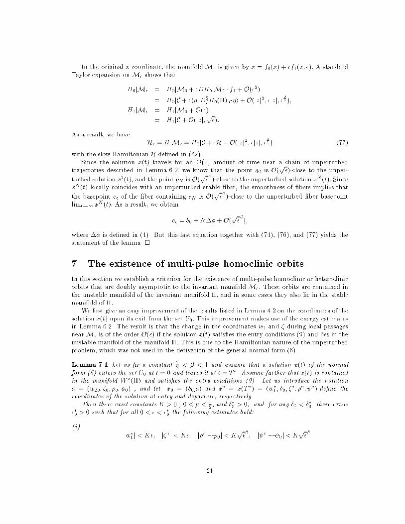
Lemma 5.2 For � � 0 and for all su�ciently small �0 � 0, the global map can be written asG�(x�) = x� +�x+ �0G1(x�; �0) +p�G2(x�; �);where Gj are C1 in their arguments, and the vector �x is de�ned in (4).Proof: We �rst observe that the mapG0:G0 ! � remains well-de�ned in the limit �0 = 0 withdomain G0 = �. The map G0 simply relates the �-limit points of unperturbed heteroclinic orbitsin W u(C) � W s(C) to their !-limit points. Therefore, for �0 = 0 we obtain G0(x�) = x� + �xfrom assumption (H6). For nonzero �0 > 0; G0 maps the �rst intersections of solutions inthe homoclinic manifolds W�0 (C) with @U0 to their second intersections with @U0: Since thesesolutions locally coincide with unperturbed �bers in W s;uloc(C); and �bers depend smoothly ontheir basepoints, we obtain that G0(x�) = x� + �x + �0G1(x�; �0): Now by assumption (H2),for x� 2 G�; the global map G�(x�) is smooth in the initial condition x� and the parameter p�.Initial conditions in the domain of G0 are at most O(��) (with � > 1=2) away from G�, and themagnitude to the perturbation in the Fenichel normal (6) is of order O(p�). This proves thestatement of the lemma. �6 Energy estimatesIn this section we shall study how the conservation of the HamiltonianH = H0+ �H1 is violatedon solutions due to the presence of general dissipative terms in equation (1). The reason for thisstudy is that we shall use the \energy" H together with the normal form variables (w2; �; �; )as coordinates to identify solutions entering the set U0 through its face w1 = �0: Similarly, weshall use the coordinates (H;w1; �; �; ) to label solutions that leave U0 through its face w2 = �0:We start with some preliminary estimates which will be needed in our main energy estimate.Lemma 6.1 Let us �x a constant 12 < � < 1 and assume that for 0 < � < �0 and �0 < �1, theestimates (9) hold for a solution x(t) which enters the set U0 at t = 0 and leaves it at t = T �:Then there exist constants L > 0 and ��0 > 0, and for any �0 < ��0 there exists ��0 > 0 such thatfor all 0 < � < ��0 we haveZ T�0 j�(t)j dt < Lp�; Z T�0 jw1(t)j dt < L�0; Z T�0 jw2(t)j dt < L�0; Z T�0 j�(t)j dt < L��; (61)where � = (1� �)=2 (see (49)).Proof: The proof of this lemma is elementary, as it follows directly from the normal form(6) and the entry conditions (9). The reader may consult Haller [21] for details. �We now formulate our main energy estimate for solutions that lie in the unstable manifold ofthe invariant manifold � and make repeated passages near �:Lemma 6.2 Suppose that x(t) is a solution of the normal form (6), which lies in the unstablemanifold of the invariant manifold �: Let q0 be the �rst intersection of x(t) with the surface @1U0and let b� = b0 + (0;p��) 2 � with b0 2 (�0; 0) 2 C be the basepoint of the unstable �ber fu(b�)which contains the point q0: Let xi(t); i = 1; : : : ; N be a chain of unperturbed heteroclinic orbitsfor the system (1) (see Fig. 6) such thatlimt!�1x1(t) = b0; limt!+1xi�1(t) = limt!�1xi(t); i = 2; : : : ; N:17

Suppose that the solution returns to @1U0 N times to intersect it in the points p1; : : : ; pN ; andto leave it again at the points q1; : : : ; qN�1: Assume further that, for some constants 12 < � < 1,0 < � < �0; and �0 < �1, the entry conditions (9) hold for the solution x(t) at each entry pointpk: (For N = 1, c2 = 0 is allowed in (9).)Then, for �0; � > 0 su�ciently small, we haveH(pN ) = H0jC + �"H(b0) + NXi=1 Z 1�1 hDH0; gixi(t) dt+O(�0; ��)# ;where 0 < � < 12 , and the "slow" Hamiltonian H is the �rst order term in the expansion of(H0 + �H1)j� near the torus C, i.e.,H = 12 �;D2IH0(�)jC��+H1jC: (62)∆φ ∆φ ∆φφ

ΠI

ε

x1(t)

2x (t)

3x (t)

0b

z

C

Figure 1: The chain of heteroclinic orbits xi(t).Proof: We start by writing H(pN ) in the formH(pN ) = H(b�) + [H(q0)�H(b�)] + N�1Xi=1 H(qi)�H(pi) + NXi=1H(pi)�H(qi�1): (63)We shall estimate the four main terms of this expression separately.To estimate the �rst term, we note that 18

H(b�) = (H0 + �H1) jb� = H0jC + �H(b0) +O(�3=2); (64)where we used the fact that DH0jC = 0 since the torus C is �lled with equilibria for � = 0:To estimate the second term in (63), we consider the \Hamiltonian" unstable �ber fug=0(b�)which intersects the surface @1U0 at a point �q0: Then, we have H(�q0) = H(b�); and the meanvalue theorem implies thatjH(q0) �H(b�)j = jH(q0)�H(�q0)j < jDH(q̂) � (q0 � �q0)j ; (65)where the point q̂ lies on the line connecting q0 and �q0. Since the unstable �bers are of class Crin the parameter �; we have jq0 � �q0j < K1�;for some integer K1: Furthermore, the gradient of H at the point q̂ satis�es the estimatejDH(q̂)j < K2�0:Therefore, the inequality in (65) can be rewritten asjH(q0) �H(b�)j < K1K2�0�: (66)To estimate the third term in (63), we note thatN�1Xi=1 H(qi) �H(pi) = N�1Xi=1 Z T�i0 _H(x(t)) dt = N�1Xi=1 Z T�i0 �DH � �!](DH) + �g�� x(t) dt (67)= �N�1Xi=1 Z T�i0 hDH0; g ix(t) dt+ O(�2 log 1� );where we used the fact that, by de�nition, DH � !](DH) = ! �!](DH); !](DH)� = 0: In (67)T �i denotes the time of ight for the solution x(t) from the point pi to qi; and hence obeys theestimate (10). (Here � > 0 is the constant de�ned in (49) and � is su�ciently small.) We shallnow estimate the three terms in the integrand on the right-hand-side of (67).Noting that DH0jC = 0, we obtain that if (w; �; �; ) are the coordinates of a point p 2 S0;then DH0(p) = A1(w; �; �; )w1 + A2(w; �; �; )w2 +A3(w; �; �; )� +A4(w; �; �; )� (68)for appropriate Cr�1 functions Ai. Using Lemma 6.1 together with (68), we obtainN�1Xi=1 Z T�i0 hDH0; g ix(t) dt = O(�0) + O(��): (69)But this last equation and the energy expression (67) shows thatN�1Xi=1 H(qi)�H(pi) = O(��0;�1+�); (70)where we used the relation (31).To complete the proof of the lemma, it remains to estimate the last sum in the expression(63). Standard \�nite-time-of- ight" Gronwall estimates imply that the perturbed solutions19

remain close to the chain of unperturbed solutions �xi(t) outside the �xed neighborhood U0of the manifoldM�: Combining this with the fact that the size of U0 is of order O(�0), we cancompute the change in energy between the points qi�1 and pi in the same way as in the �rst lineof equation (67). We then obtainNXi=1H(pi) �H(qi�1) = � NXi=1 Z 1�1 hDH0; gi jxi(t) dt+O(��0): (71)But (63), (64), (70), and (71) together prove the statement of the lemma. �In the following lemma we estimate the energy of a point sN 2 W sloc(M�) \ @1U0 whichhas the same (z; �; �) coordinates as the point pN on the incoming solution x(t): We will usethis estimate to compute the energy di�erence between the point pN and its projection on theunstable manifold of M�:Lemma 6.3 Suppose that x(t) is a solution of the normal form and let the points p1; : : : ; pN andq0; : : : ; qN�1 be de�ned as in Lemma 6.2. Suppose that the assumptions of that lemma hold andc� 2 M� is the basepoint of a stable �ber fs(c�) such that for the point sN = fs(c�) \ @1U0;(�pN ; �pN ; pN ) = (�sN ; �sN ; sN ): (72)Then, for the energy of the point sN , we have the expressionH(sN ) = H0jC + �H(b0 + N��) + O(��0; �1+�=2); (73)where the phase shift vector �� is de�ned in (4) and the slow Hamiltonian H is de�ned in (62).Proof: Since the entry estimates (9) are assumed to hold for the incoming solution x(t);equation (72) implies that the stable �ber fs(c�) containing sN is locally O(��)-close to anotherstable �ber with basepoint on the invariant manifold �: By the smoothness of �bers with respectto the parameter �; this implies that the basepoint c� is O(��) close to �; i.e.,jzc� j < K7�� : (74)Now sN lies at a distance of order O(�0) from the invariant manifoldM�; so by the smoothnessof individual stable �bers we have(�c� ; �c�) = (�sN ; �sN ) + O(�0): (75)We now relate the energy of the basepoint c� to the energy of the point sN . Let the point sh bethe intersection of the \Hamiltonian" �ber fsg=0(c�) with the surface @1U0: Then, applying themean value inequality with some point s� lying on the line segment connecting sN and sh, wecan writejH(sN )�H(c�)j = ��H(sN ) �H(sh)�� < jDHjs� ��sN � sh�� < jDHjs�K8� < K8K9�0�;which yields H(sN ) = H(c�) + O(�0�): (76)Hence, to �nd an approximation for the energy of the point sN ; we have to compute the energyof the �ber basepoint c�: For this purpose, we have to �nd the restriction H� of the HamiltonianH to the manifoldM�. 20

In the original x coordinate, the manifoldM� is given by x = f0(x) + �f1(x; �): A standardTaylor expansion on M� shows thatH0jM� = H0jM0 + �DH0jM0 � f1 + O(�2)= H0jC + �h�;D2IH0(�)jC�i+O(jzj2; �jzj; � 32 );H1jM� = H1jM0 +O(�)= H1jC +O(jzj;p�):As a result, we have H� = HjM� = H0jC + �H+ O(jzj2; �jzj; � 32 ) (77)with the slow Hamiltonian H de�ned in (62).Since the solution x(t) travels for an O(1) amount of time near a chain of unperturbedtrajectories described in Lemma 6.2, we know that the point q0 is O(p�)-close to the unper-turbed solution x1(t); and the point pN is O(p��)-close to the unperturbed solution xN (t): SincexN (t) locally coincides with an unperturbed stable �ber, the smoothness of �bers implies thatthe basepoint c� of the �ber containing sN is O(p��)-close to the unperturbed �ber basepointlimt!1 xN (t): As a result, we obtainc� = b0 +N��+O(p��);where �� is de�ned in (4). But this last equation together with (74), (76), and (77) yields thestatement of the lemma. �7 The existence of multi-pulse homoclinic orbitsIn this section we establish a criterion for the existence of multi-pulse homoclinic or heteroclinicorbits that are doubly asymptotic to the invariant manifold M�: These orbits are contained inthe unstable manifold of the invariant manifold �, and in some cases they also lie in the stablemanifold of �:We �rst give an easy improvement of the results listed in Lemma 4.2 on the coordinates of thesolution x(t) upon its exit from the set U0: This improvement makes use of the energy estimatesin Lemma 6.2. The result is that the change in the coordinates w1 and � during local passagesnear M� is of the order O(�) if the solution x(t) satis�es the entry conditions (9) and lies in theunstable manifold of the manifold �: This is due to the Hamiltonian nature of the unperturbedproblem, which was not used in the derivation of the general normal form (6).Lemma 7.1 Let us �x a constant 12 < � < 1 and assume that a solution x(t) of the normalform (6) enters the set U0 at t = 0 and leaves it at t = T �. Assume further that x(t) is containedin the manifold W u(�) and satis�es the entry conditions (9). Let us introduce the notationa = (w20; �0; �0; 0) , and let x0 = (�0;a) and x� = x(T �) = (w�1; �0; ��; ��; �) de�ne thecoordinates of the solution at entry and departure, respectively.Then there exist constants K > 0 , 0 < � < 12 ; and ��0 > 0, and for any �0 < ��0 there exists��0 > 0 such that for all 0 < � < ��0 the following estimates hold:(i) jw�1j < K�; j��j < K�; j�� � �0j < Kp��; j � � 0j < Kp��:21

(ii) jDaw�1j < K��; jDa �� � (0; 1; 0; 0)j< K��;jDa �� � (0; 0; 1; 0)j< K��; jDa � � (0; 0; 0; 1)j < K��:(iii) jD��w�1j < K��; jD����j < K��; jD�� ��j < K��; jD�� �j < K��:Proof: Consider the point q� 2 W uloc(�) for which w1q� = 0; �q� = 0; and (�q� ; q�) =(�x� ; x�) hold. By (i) of Lemma 4.2, the points q� and x� are O(��) close. To determinethe energy of the point q�; we consider the unstable �ber fu(b�) which contains q�: For zerodissipation (g � 0), the energy of the basepoint b� of the �ber fug=0(b�) can be written in theform H(b�) = H0jC +O(�);where we used (77). Since the energy is constant on �bers for g � 0;we immediately obtain H(q�) = H0jC + O(�): (78)This equation remains valid for nonzero dissipation, since unstable �bers perturb by an O(�)amount when we add the dissipative terms. Also, setting q1 = x� in Lemma 6.2, we obtain thatH(x�) = H0jC +O(�):This last equation together with (78) and the mean value inequality givesK10� > jH(q�)�H(x�)j = ����DH(q̂) � q� � x�jq� � x�j ���� jq� � x�j > K11�0 jq� � x�j ; (79)where q̂ is an appropriate point on the line connecting the points q� and x�: Here we made use ofthe facts that the diameter of the set U0 is of the order O(�0) and the perturbed ow intersectsthe line between q� and x� with O(1) transversality due to the geometry of the unperturbedHamiltonian ow. We rewrite (79) in the formjq� � x�j < K10K11�0 �: (80)Since the transformation from the (y; z; �; �) coordinates to the (w; �; �; ) coordinates is a dif-feomorphism with norm of order O(1), this last expression implies thatjw�1j < K12�; (81)since w1q� = 0. Furthermore, as the unstable �bers are straight lines for the local normal form(6), �q� = 0 must hold, since the basepoint of the unstable �ber containing q� lies in the invariantmanifold � which obeys � = 0: As a result, (81) impliesj��j < K13�;which, together with the estimate (81) proves the �rst two inequalities in statement (i) of thelemma. The remaining inequalities are just restatements of the results listed in Lemma 4.2. �The following de�nition describes the types of orbits that we will be interested in �nding.De�nition 7.1 Let us consider a point b0 2 C and let j = fjigNi=1 be a sequence of +1's and�1's. An orbit x� of system (1) is called an N -pulse homoclinic orbit with basepoint b0 andjump sequence j; if for some 0 < � < 12 and for � > 0 su�ciently small,22

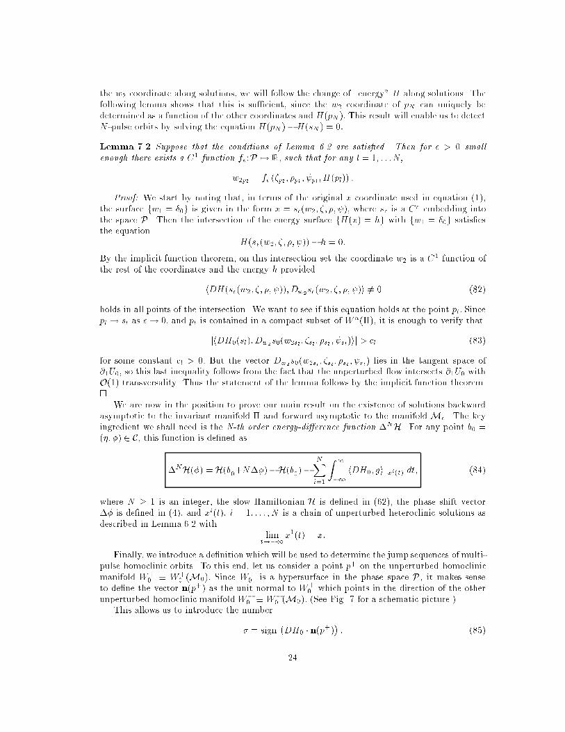
(i) x� intersects an unstable �ber fu(b�) with basepoint b� = b0 + O(��) 2 �,(ii) x� intersects a stable �ber fs(c�) with basepoint c� = b0 + N�� + O(��) 2 M� such thatdist(c�;�) = O(�).(iii) Outside a small �xed neighborhood of the manifold M�; the orbit x� is order O(��) close toa chain of unperturbed heteroclinic solutions xi(t); i = 1; : : : ; N , such thatlimt!�1x1(t) = b0; limt!+1xi�1(t) = limt!�1xi(t); i = 2; : : : ; N:Furthermore, for k = 1; : : : ; N and for all t 2 R we havexk(t) 2 � W+0 (C) if jk = +1;W�0 (C) if jk = �1:To illustrate the above de�nition, we show a three-pulse homoclinic orbit schematically inFig. 7.∆φ ∆φ ∆φφ

Π

x1(t)

2x (t)

3x (t)

εb 0b

uf ( )εb

xεs

f ( )εc

εc

I

ε

Figure 2: 3-pulse homoclinic orbit to the manifold M� with jump sequence j = f+1;�1;+1gand with basepoint b�.To �nd N -pulse orbits of the type described in De�nition 7.1, it is clearly enough to �ndconditions under which the points pN 2Wu(�) and sN 2W sloc(M�) coincide. By construction,these points have the same w1; �; �; and coordinates, so they coincide if their w2 coordinatesare equal, i.e., the w2 coordinate of pN is zero. However, instead of following the evolution of23

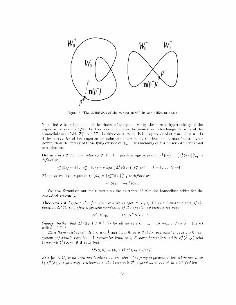
the w2 coordinate along solutions, we will follow the change of \energy" H along solutions. Thefollowing lemma shows that this is su�cient, since the w2 coordinate of pN can uniquely bedetermined as a function of the other coordinates and H(pN ): This result will enable us to detectN -pulse orbits by solving the equation H(pN )�H(sN ) = 0:Lemma 7.2 Suppose that the conditions of Lemma 6.2 are satis�ed. Then for � > 0 smallenough there exists a C1 function f�:P 7! R; such that for any l = 1; : : :N;w2pl = f� (�pl ; �pl ; pl;H(pl)) :Proof: We start by noting that, in terms of the original x coordinate used in equation (1),the surface fw1 = �0g is given in the form x = s�(w2; �; �; ); where s� is a Cr embedding intothe space P. Then the intersection of the energy surface fH(x) = hg with fw1 = �0g satis�esthe equation H(s�(w2; �; �; ))� h = 0:By the implicit function theorem, on this intersection set the coordinate w2 is a C1 function ofthe rest of the coordinates and the energy h providedhDH(s�(w2; �; �; )); Dw2s�(w2; �; �; )i 6= 0 (82)holds in all points of the intersection. We want to see if this equation holds at the point pl: Sincepl ! sl as �! 0; and pl is contained in a compact subset of W u(�), it is enough to verify thatjhDH0(sl); Dw2s0(w2sl; �sl; �sl ; sl)ij > cl (83)for some constant cl > 0: But the vector Dw2s0(w2sl; �sl; �sl ; sl) lies in the tangent space of@1U0; so this last inequality follows from the fact that the unperturbed ow intersects @1U0 withO(1) transversality. Thus the statement of the lemma follows by the implicit function theorem.� We are now in the position to prove our main result on the existence of solutions backwardasymptotic to the invariant manifold � and forward asymptotic to the manifold M�. The keyingredient we shall need is the N-th order energy-di�erence function �NH. For any point b0 =(�; �) 2 C, this function is de�ned as�NH(�) = H(b0+N��)�H(b0)� NXi=1 Z 1�1 hDH0; gi jxi(t) dt; (84)where N � 1 is an integer, the slow Hamiltonian H is de�ned in (62), the phase shift vector�� is de�ned in (4), and xi(t), i = 1; : : : ; N is a chain of unperturbed heteroclinic solutions asdescribed in Lemma 6.2 with limt!�1x1(t) = x:Finally, we introduce a de�nition which will be used to determine the jump sequences of multi-pulse homoclinic orbits. To this end, let us consider a point p+ on the unperturbed homoclinicmanifold W+0 � W+0 (M0): Since W+0 is a hypersurface in the phase space P, it makes senseto de�ne the vector n(p+) as the unit normal to W+0 which points in the direction of the otherunperturbed homoclinic manifoldW�0 � W�0 (M0): (See Fig. 7 for a schematic picture.)This allows us to introduce the number� = sign �DH0 � n(p+)� : (85)24

W

p+

(p )+n

+W0−W0

p+

−W0

+0

(p )+nFigure 3: The de�nition of the vector n(p+) in two di�erent cases.Note that � is independent of the choice of the point p+ by the normal hyperbolicity of theunperturbed manifoldM0: Furthermore, � remains the same if we interchange the roles of thehomoclinic manifoldsW+0 and W�0 in this construction. It is easy to see that � = �1 (� = +1)if the energy H0 of the unperturbed solutions encircled by the homoclinic manifold is higher(lower) than the energy of those lying outside ofW+0 : This meaning of � is preserved under smallperturbations.De�nition 7.2 For any value �0 2 Tm; the positive sign sequence �+(�0) = f�+k (�0)gNk=1 isde�ned as�+1 (�0) = +1; �+k+1(�0) = �sign ��kH(�0)� �+k (�0); k = 1; : : : ; N � 1:The negative sign sequence ��(�0) = f��k (�0)gNk=1 is de�ned as��(�0) = ��+(�0):We now formulate our main result on the existence of N -pulse homoclinic orbits for theperturbed system (1).Theorem 7.3 Suppose that for some positive integer N , �0 2 Tm is a transverse zero of thefunction �NH; i.e., after a possible reindexing of the angular variables � we have�NH(�0) = 0; D�1�NH(�0) 6= 0:Suppose further that �kH(�0) 6= 0 holds for all integers k = 1; : : : ; N � 1; and let � = (�1; ~�)with ~� 2 Tm�1:Then there exist constants 0 < � < 12 and C� > 0; such that for any small enough � > 0; thesystem (2) admits two, 2m � 1{parameter families of N -pulse homoclinic orbits x�� (~�; �0) withbasepoints b�� (~�; �0) 2 � such thatb�� (~�; �0) = (�0 +O(��); I0 +p��0):Here j�0j < C� is an arbitrary localized action value. The jump sequences of the orbits are givenby ��(�0); respectively. Furthermore, the basepoints b�� depend on ~� and �� in a C1 fashion.25

Proof: For � > 0 and �0 > 0 su�ciently small, let us consider a solution x(t) which lies inthe component W u+0 (�) of the unstable manifold of the invariant manifold �: (W u+0 (�) denotesthe connected component ofW u0 (�) that perturbs from the homoclinic manifoldW+0 :) We followx(t) up to its �rst intersection with the surface w2 = �0. We denote this intersection point by q0and note that it lies on an unstable �ber fu(b�) with some basepoint b� = (�0;p��0) 2 � (seeFig. 7). We then follow the solution as it leaves the neighborhood U0 of the manifoldM� and,φ

Π0b

I

ε

0q2w =δ 0

uf ( )

0b

1qw1

=δ 0

1p

2w =δ 0

x(t)

z

sf ( )1b

1b

1s

Figure 4: The geometry of the proof of Theorem 6.2.by standard Gronwall estimates, returns and intersects the subset jw1j = �0 of the surface @1U0:We denote this second intersection point by p1 (see Fig. 7). Since the unstable �bers are straightin the (w; �; �; ) coordinates, we have j�q0 j = 0 by construction. Then q0 is clearly contained inthe domain G� of the global map G� (see (59) and (60)) and we can write p1 = G�(q0):Since the manifoldW s+loc(M�) is a graph over the variables (w1; �; �; ), there exists a uniquepoint s1 2W s+loc(M�) \ @1U0 as de�ned in Lemma 6.3. In particular, we have(�s1 ; �s1; s1) = (�p1 ; �p1 ; p1) :According to Lemma 7.2, p1 � s1 holds if and only ifH(p1)�H(s1(p1)) = 0; (86)where we view s1 as a function of p1: Note that the right-hand-side of equation (86) is Cr in thevariable p1:By standard Gronwall estimates, the point p1 of the solution x(t) is O(�)-close to a stable�ber fs(b1) with basepoint b1 = b� + �� 2 � (see Fig. 7). As a result, it satis�es the entry26

conditions listed in (9) with � = 1 and c2 = 0. Consequently, Lemma 6.2 applies with n = 1 andgives H(p1(b�)) = H0jC + � �H(b0) + Z 1�1 hDH0; gix1(t) + O(�0; ��)� (87)for an appropriate constant 0 < � < 12 : Furthermore, Lemma 6.3 with n = 1 also applies andyields H(s1(b�)) = H0jC + �H(b0 +��) + O(��0; � 32 ): (88)Since b� = b0 + O(p�) = (�0;p��0); for any � > 0 we can use (87), (88), and the de�nition of�1H in (84) to rewrite the energy equation (86) as�1H(�0) + �0F1(p1(b�); �0; ��) + ��G1(p1(b�); �0; ��) = 0 (89)with p1 = (0; w2p1; �p1 ; �p1 ; p1) = G�(q0). The points b0 and p1 are related byp1(b0) = G� � P u� (b0); (90)where P u� :W u+loc (�) \ @1U0 ! � is the �ber projection map that maps the intersection pointsof unstable �bers in W u+loc (�) with the surface @1U0 to the basepoints of these �bers. By thesmoothness of �bers in W u+loc (�), the function P u� is a Cr map. By Lemma 5.2, G� is a C1 mapfrom G� to P: As a result, equation (90) shows that p1 is a C1 function of b0: This in turn impliesthat the right-hand-side of the energy equation (89) is of class C1 with respect to b0; becausethe functions F1 and G1 are smooth in p1, as we observed after formula (86), and �1H is a C1function.Assume now that N = 1 holds in the statement of the theorem. Then, by the assumptions ofthe theorem, b0 = (�0;p��0) with any 0 < j�0j � C� is a solution of equation (89) for �0 = � = 0:We want to apply the implicit function theorem to argue that this solution can be continued for�; �0 > 0: Setting � = 0; and di�erentiating (89) with respect to the �1 coordinate of b0 yieldsD�1 ��1H(�0) + �0F1(p1(b0); �0; 0)� = D�1�1H(�0)+�0 Dp1F1; DG0DP u0 D�01T �10 � jb0: (91)Here, �0 = (�01; ~�0) and T� is the normal form transformation constructed in Lemma 3.1. NowD�1�1H is a continuous function, and we have D�1�1H(�0) 6= 0 by assumption. Hence forsu�ciently small �0 > 0; (91) is nonzero. (This follows by recalling that the right-hand-side of(91) continuous in b0 and the termDp1F1; DG0DP u0 D�01T �10 � jb0remains bounded as �0 ! 0 by Lemma 5.2.) Thus (89) admits a solution ��1(~�; �0; �0) = �01 +O(�0) for �0 > 0 small and � = 0. We �x �0 su�ciently small, substitute the solution ��1 backinto equation (89). The derivative of the left-hand-side of the resulting equation with respect to�1 is given by D�1�1H �(��1; ~�)�+ �0 Dp1F1; DG�DP u� D�01T �1� �+�� rp1G1; DG�DP u� D�01T �1� � :By Lemma 5.2, this derivative is continuous at � = 0; and is also nonzero by assumption. Thusequation (89) admits a solution �̂1(~�; �0; �0; �) = �01 + O(�0; ��) for � > 0 su�ciently small.27

For any �xed �, the solution should not depend on �0; which is just an auxiliary parameter tomeasure the size of the neighborhood U0 that we have worked in. Therefore, we have d�̂1=d�0 = 0;implying �̂1(~�; �0; �) = �01+O(��): This proves the existence of the orbit familyx+� (~�) for N = 1.The smoothness of x+� (~�) with respect to �� follows from Lemma 5.2.Assume now that N > 1 in the statement of the theorem. Then, by the conditions of thetheorem, we see that for � and �0 su�ciently small the energy equation (89) cannot be satis�ed,so the solution x(t) does not intersect the local stable manifold ofM� upon its �rst return to theneighborhood U0: Using (87), (88), and the compactness of the solid m-torus [�C�; C�]m �Tm;we conclude the existence of positive constants K(1)1 and K(1)2 such thatK(1)1 � < jH(p1) �H(s1)j < K(1)2 �: (92)Now the mean value theorem implies thatjH(p1) �H(s1)j = �����DH(p�1); p1 � s1jp1 � s1j����� jp1 � s1j> C(1)2 jp1 � s1j ; (93)where p�1 is a point on the line connecting p1 and s1; and the existence of C(1)2 > 0 follows froman argument similar to that leading to estimate (83). At the same time, the mean value theoremimplies that jH(p1)�H(s1)j < C(1)1 jp1 � s1j (94)for some constant C(1)1 > 0; so it follows from (92)-(94) thatK(1)1 �C(1)1 < jp1 � s1j < K(1)2 �C(1)2 : (95)This last expression in (95) immediately shows that the coordinates (w2p1 ; �p1 ; �p1 ; p1) satisfythe entry conditions in (9) (because the normal form coordinates of the point s1 satisfy w1s1 = �0;w2s1 = 0; and j�s1 j = O(�)). Consequently, the point p1 is contained in the domain L� of thelocal map L�, and we can write q1 = L�(p1) where q1 is the next intersection of the solution x(t)with the surface @1U0:Let p2 denote the intersection of the solution x(t) with the surface @1U0 upon its second returnto the neighborhood U0: (The existence of p2 is guaranteed by the usual Gronwall estimates for� > 0 small enough.) We again have a point s2 2W sloc(M�) \ @1U0 such that(�s2 ; �s2; s2) = (�p2 ; �p2 ; p2) :Again, the solution x(t) gives rise to a 2-pulse homoclinic orbit ifH(p2) �H(s2(p2)) = 0;or, alternatively, �2H(�0) + �0F2(p2(b�); �0; ��) + ��G2(p2(b�); �0; ��) = 0; (96)where we used Lemmas 6.2 and 6.3. As in equation (89), the functions F2 and G2 are C1 in theirarguments. Since p2(b�) = G� � L� �G� � P u� (b�);28

we see that for � � 0; p2 is a C1 function of b� and �� by Corollary 5.1 and Lemma 5.2. Thenjust as in the case of N = 1; the implicit function theorem applied to (96) implies the existenceof the orbit family x+� (~�; �0) for N = 2:The proof for any N > 2 follows the same steps as that of the case N = 2. The existence ofthe other N -pulse homoclinic orbit family x�� (~�; �0) for any N � 1 follows from the fact that anidentical construction can be repeated for solutions contained in W u�(�): Therefore, it remainsto show that the jump sequences of the two families x�� (~�) are indeed given by the sign sequences��(�0); respectively. We sketch the argument for x+� only since the argument for x�� is identical.Consider an N -pulse homoclinic orbit x+� : By construction it makes its �rst pulse in thevicinity of the unperturbed manifold W+0 (C), hence the �rst element of its jump sequence isindeed �+1 (�0) = +1: For small �; �0 > 0; at the �rst re-entry point p1 we havesign (H(s1) �H(p1)) = sign [�(�1H(�0 +O(�0; ��))+�0FN (pN (b+� ); �0; ��)+��GN (pN (b+� ); �0; ��))]= sign ��1H(�0)� : (97)If this quantity is positive, then at the point p1 the solution x(t) has higher energy than nearbypoints in the hypersurface W s+loc(M�): Recalling the meaning of the constant � (see (85)), we canconclude that � sign ��1H(�0)� = +1 implies that the solution x(t) stays near the homoclinicmanifoldW+0 (C), whereas � sign ��1H(�0)� = �1 causes the solution to perform its second jumpin the vicinity of the manifoldW�0 (C): Therefore, the second element in the jump sequence of x+�is given by �+2 (�0) as de�ned in De�nition 7.2. The remaining elements of the jump sequence ofx+� are constructed recursively in the same fashion, hence they coincide with the correspondingelements of the sign sequence �+(�0) in De�nition 7.2. This completes the proof of the theorem.� In the following we describe two situations in which the above theorem can be applied: Forsimplicity, we will consider the case m = 1, i.e., we assume that the manifold � is two-dimensional,hence the center manifoldM0 of the unperturbed system is 2n+ 2 dimensional.To �nd the asymptotic behavior of multi-pulse orbits, one has to have some knowledge of thedynamics on the two-dimensional manifoldM�: A straightforward Taylor expansion shows (see,e.g., Haller and Wiggins [15]) that near the resonant circle C the ow on � satis�es the equations_� = p�D�Hg(�; �) + O(�); (98)� = �p�D�Hg(�; �) + O(�);with Hg(�; �) = H(�; �)� Z �0 gI jC(u) du (99)= 12D2IH0(C)�2 +H1jC(�) � Z �0 gIjC(u) du;where the slow Hamiltonian H is de�ned in (62) and gI is the I-component of the perturbationterm g in equation (1). As seen from (98), for �nite times the solutions on the manifold � areapproximated with an error of order O(p�) by the level curves of the function Hg: (We notethat, in general, the ow generated by Hg is only locally Hamiltonian, i.e., it does not admit asingle valued Hamiltonian on �: We seleted the HamiltonianHg in a way such that it generatesthe leading order Hamiltonian terms through the canonical symplectic form d�^ dI:)29

Theorem 7.4 Suppose that m = 1 and the conditions of Theorem 7.3 hold. Assume further thatthe curve f� = �0g � � intersects transversely the unstable manifold of a hyperbolic �xed pointp0 2 � of the Hamiltonian Hg. Let (0; 0; �0; �0) be the coordinates of the point p0 and assumethat for any small enough jzj > 0 and � > 0; the point (y0; z; �0; �0 + N��) 2 M� lies in thedomain of attraction of an invariant set S� � �:Then, for � > 0 su�ciently small, there exists 0 < � < 12 such that system (2) admits two N -pulse homoclinic orbits x�� with basepoints b�� = p0+O(��) 2 � and with jump sequences ��(�0);respectively. Both orbits are backward asymptotic to a hyperbolic �xed point p� = p0+O(p�) � �and forward asymptotic to the invariant set S�.Proof: By Theorem 7.3 we immediately obtain the existence of a curve B� � � which containsbasepoints for N -pulse homoclinic orbits of the type of x�� : From the proof of that theorem it isalso clear that the curve B� is C1 O(��)-close to the line f� = �0g: As a result, it will intersectthe unstable manifold of the �xed point p�, which perturbs from p0 under the e�ect of dissipativeand higher order Hamiltonian terms. Then, by the invariance properties of unstable �bers, thisintersection point is a basepoint for an N -pulse homoclinic orbit that backward asymptotes top�. Finally, the invariance properties of stable �bers imply that the N -pulse homoclinic orbitasymptotes to the attracting set S� in forward time. �In applications system (1) frequently depends on parameters. Varying these parameters on acodimension-one subset of the parameter space, it is possible to construct multi-pulse homoclinicorbits which have their basepoints precisely on an equilibrium point p� contained in the invariantmanifold �: If, in addition, the attracting set S� assumed in the previous theorem is just the �xedpoint p�, then the multi-pulse homoclinic orbit obtained in this fashion is an orbit homoclinic top� itself.Theorem 7.5 Suppose that m = 1, system (1) depends on a vector � 2 Rp of system parametersin a Cr fashion, and V � Rp is an open set. Assume further that(i) For any � 2 V the Hamiltonian Hg has a nondegenerate equilibrium (i.e., no zero eigenval-ues) p0(�) = (�0(�); �0(�)) 2 �:(ii) For some positive integer N and for some parameter value �0 2 V , �0(�0) satis�es theconditions of Theorem 7.3.(iii) D��NH(�0(�); �)j�=�0 6= 0:(iv) For small enough jzj and � > 0; the point (y0; z; �0; �0 + N��) 2 M� lies in the domainof attraction of an asymptotically stable �xed point p� � � of system (98) which perturbsfrom the �xed point p0:Then there exists a codimension-one setM+ � Rp�Rnear the point (�0; 0) such that for everyparameter value (�; �) 2 M; the system (2) admits an N -pulse homoclinic orbit x+� homoclinicto the point p�. The basepoint for this orbit is p� and the jump sequence of the orbit is given by�+(�0(�0)): There also exists another codimension one set M� � Rp � R which yields similarhomoclinic orbits with jump sequence ��(�0(�0)):Proof: The main steps in the proof of this theorem are similar to those in the proof of Theorem7.3. However, we now want to force the perturbed �xed point p� to be a solution of the equation�NH (p�(�);�) + �0FN (pN (p�(�)); �0; ��; �) + ��GN (pN (p�(�)); �0; ��; �) = 030

with p�(�) = (�0(�) +p�P1(�; �); �0(�) +p�P2(�; �)) : Using (iv) and the implicit functiontheorem, we see that this equation can again be solved in two steps to obtain a solution��(�) = �0 +O(��): �We note that in the case of n = 0 the above theorem is identical to the one obtained inHaller and Wiggins [18] for the existence of �Silnikov-type orbits in two-degree-of-freedom systems.Another situation in which multi-pulse �Silnikov-type orbits may occur is when an equilibriump� 2 � of the perturbed system is a saddle restricted to the manifold �, but when viewed withinthe center manifoldM�, it also admits n pairs of complex eigenvalues with negative real parts.Theorem 7.6 Suppose that m = 1 and system (1) depends on a parameter � 2 R in a Crfashion. Let V 2 R be an open set and assume that(i) The Hamiltonian Hg has a nondegenerate equilibrium (i.e., no zero eigenvalues) p0(�) =(�0(�); �0(�)) 2 �: If p�(�) 2 � is the corresponding equilibrium of the perturbed system(1), then the manifold W s(p�(�))\M� is codimension one within the center manifold M�.(ii) The \size" of W s(p�(�)) is of order O(�q) with 0 � q < 1, i.e., it intersects a surfacejzj = K�q transversely.(iii) For some positive integer N and for all � 2 V , there exists a function �0(�) which satis�esthe conditions of Theorem 7.3.(iv) The line f� = �0(�)g � � intersects transversely the unstable manifold of the �xed pointp0 2 � of the slow Hamiltonian.(v) If (0; 0; �0(�); �0(�)) are the coordinates of this transverse intersection point, then the point(0; 0; �0; �0(�) + N��(�)) crosses the stable manifold of p0 transversely as � is variedthrough �0.Then there exists a codimension one set M+ � R2 near the point (�0; 0) such that for everyparameter value (�; �) 2M; the system (1) admits an N{pulse homoclinic orbit x+� to the pointp�(�). The basepoint for this orbit lies in W u(p�)\� and the jump sequence of the orbit is givenby �+(�0(�0)): There also exists another codimension one set M� � R2 which yields similarhomoclinic orbits with jump sequence ��(�0(�0)):Proof: Again, the main steps in the proof of this theorem coincide with those in the proof ofTheorem 7.3. The new element is that we want to force the stable �ber, which is intersected bythe N -pulse homoclinic orbit, to lie on the stable manifold of the perturbed �xed point p�. Atthe same time, we do not require the basepoint of the N -pulse orbit to coincide with p� as in theprevious theorem, but rather we allow the basepoint to be any point in the set W u(p�) \�.As in the proof of Theorem 7.3, we �rst solve the equation�NH (p�(�);�) + �0FN (pN (p�(�)); �0; ��; �) + ��GN (pN (p�(�)); �0; ��; �) = 0to obtain a solution ��(�; �) = �0(�) + O(��). By assumption (iv) and by the C1 dependence of�� on �� (cf. Theorem 7.3), the curve f� = ��(�; �)g intersects the unstable manifold of the �xedpoint p�(�) transversely in a point�p(�; �) = (�0(�) +O(��); �0(�) +O(��)) 2 �:We know (cf. De�nition 7.1) that the N -pulse solution with basepoint �p(�; �) intersects a stable�ber fs(p̂(�; �)) whose basepoint has the (y; z; �; �) coordinatesp̂(�; �) = (0;O(�); �0(�) +O(��); �0(�) + ��(�) + O(��)) 2M�: (100)31

Furthermore, by assumption (ii), in a vicinity of the manifold � the stable manifold of p� can bewritten as a graph over either the (�; z) or the (�; z) variables. Considering the former case (thelatter can be dealt with in the same way), we obtain that near � a compact subset of W s(p�(�))satis�es an equation of the form � = m1(�; �) + zm2(�; z; �; �); (101)where mj are of class Cr and � = m1(�; �) is the local equation of the stable manifold of p0 onthe manifold �.Our goal is to �nd parameter values for which the stable �ber basepoint p̂(�; �) is containedin the stable manifold of the �xed point p�(�). From (100) we see that dist(p̂(�; �);�) = O(�);and hence by assumption (ii) of the theorem, p̂(�; �) lies in the domain where W s(p�(�)) satis�es(101). Then formulas (100) and (101) give the equation�0(�) +��h�(�; �)�m1 (�0(�) + ��h�(�; �); �)��hz(�; �)m2 (�0(�) + ��h�(�; �); �hz(�; �); �; �) = 0; (102)where the functions h�, h�, and hz are di�erentiable in � and ��. Now by assumption (v), weknow that �0(�0)�m1 (�0(�0); �0) = 0; D� [�0(�) �m1 (�0(�); �)]�=�0 6= 0;thus the implicit function theorem guarantees a solution ��(�) = �0 + O(��) to equation (102).This completes the proof of the theorem. �8 Geometry of the unstable manifold of �Using the methods of the proof of Theorem 7.3, we can follow any particular solution in theunstable manifold of the manifold � on time scales of order O(log 1=p�); while the unstablemanifold makes a �nite number of \jumps". The following de�nition will be used to distinguishbetween di�erent types of jumping orbits within the unstable manifold of �:De�nition 8.1 Let us consider a point b0 2 C and let j = fjigNi=1 be a sequence of +1's and�1's. An orbit x� of system (1) is called an N -pulse orbit with basepoint b0 and jump sequencej; if for some 0 < � < 12 and for � > 0 su�ciently small,(i) x� intersects an unstable �ber fu(b�) with basepoint b� = b0 + O(��) 2 �,(ii) Outside a small �xed neighborhood of the manifold M�; the orbit x� is order O(p�) close toa chain of unperturbed heteroclinic solutions xi(t); i = 1; : : : ; N , such thatlimt!�1x1(t) = b0; limt!+1xi�1(t) = limt!�1xi(t); i = 2; : : : ; N:Furthermore, for k = 1; : : : ; N and for all t 2 R we havexk(t) 2 � W+0 (C) if jk = +1;W�0 (C) if jk = �1:We have the following result for the existence of N -pulse orbits.32

Theorem 8.1 Suppose that for some positive integer N and for some �0 2 Tm we have�kH(�0) 6= 0; k = 1; : : : ; N � 1:Then, for � > 0 su�ciently small there exist constants 0 < � < 12 and C� > 0; such thatfor any 0 � j�0j < C�; the system (2) admits two of N -pulse orbits x�� with basepoint b� 2 �such that �b� = �0 +O(��) and �b� = �0. The jump sequences of the orbits are given by ��(�0);respectively.Proof: Using the assumption of the theorem and the arguments from the proof of Theorem7.3, we immediately conclude that for � > 0 small enough the inequalities�kH(�0) + �0Fk(pk(b�); �0; ��) + ��Gk(pk(b�); �0; ��) 6= 0hold for k = 1; : : : ; N � 1: As a result, the unstable manifoldW u(�) contains two N -pulse orbitswith basepoint (�0; �0): The jump sequences of these orbits can be found in exactly the sameway as in the proof of Theorem 7.3. �The above result can be used in examples to study the \disintegration" of the unstablemanifold of �. In particular, in the process of its jumping around �; the open sets in themanifold W u(�) depart from each other and follow di�erent jump sequences. This results inobservable irregular transient behavior near the broken homoclinic structure, even if there areno chaotic invariant sets created by the perturbation. We will use this fact when we apply ourresults to a discretization of the forced NLS equation.9 An alternative formulation of the resultsIt may happen that the unperturbed limit of system (1) admits an invariant which o�ers a moreconvenient base for perturbation methods than the Hamiltonian H0. For this reason, we alsopresent an easy modi�cation of our results that uses some other integral of the unperturbed limit.This alternative formulation will prove very useful in our study of the discretized NLS equationin the next section.We consider a modi�cation of system (1) in the form_x = !](DH0(x)) + �g(x); (103)and assume that for � = 0, there exists a Cr+1 function K0:P ! R, which is independent of theHamiltonian H0 and Poisson commutes with H0, i.e.,fH0;K0g = !(!](DH0); !](DK0)) = 0: (104)This last condition implies that the ows generated by H0 and K0 through the symplectic form! commute. We also assume that on the circle of equilibria C,DK0jC = 0: (105)Following the de�nition of the energy-di�erence functions in (84), we introduce the function�NK(�) = � NXi=1 Z 1�1 hDK0; gi jxi(t) dt: (106)We also rede�ne the number � in (85) as� = sign �DK0 �n(p+)� ; (107)as well as the sign sequences in De�nition 7.2: 33

De�nition 9.1 For any value �0 2 Tm; the positive sign sequence �+(�0) = f�+k (�0)gNk=1 isde�ned as�+1 (�0) = +1; �+k+1(�0) = � sign ��kK(�0)��+k (�0); k = 1; : : : ; N � 1:The negative sign sequence ��(�0) = f��k (�0)gNk=1 is de�ned as��(�0) = ��+(�0):We then have the following result.Theorem 9.1 The statements of Theorems 7.3-7.6 also hold if we replace the energy-di�erencefunction �NH with the function �NK de�ned in (106) and we use the de�nition of sign sequencesgiven in De�nition 9.1.Proof: Our estimates for the local dynamics near the manifold M0 in section 4 as well asLemma 6.1 make no use of the HamiltonianH1, hence they hold without change. Lemma 6.2 canalso be proved using the function K0 instead of H0 noting that H1 � 0. Indeed, equation (105)ensures that K0 has the same type of Taylor expansion near the resonant circle C as H0 does.Furthermore, the change of K0 along perturbed solutions during passages near the manifoldM�can be computed as (cf. (67))N�1Xi=1 K0(qi)�K0(pi) = N�1Xi=1 Z T�i0 _K0(x(t)) dt = N�1Xi=1 Z T�i0 �DK0 � �!](H0) + �g��x(t) dt= N�1Xi=1 Z T�i0 [fK0;H0g+hDK0; gi] x(t) dt (108)= �N�1Xi=1 Z T�i0 hDK0; g ix(t) dt;where we used (104). Moreover, this last integral can again be approximated (with error of orderO(�0)) by an improper integral as in (71), because by (105), jDK0j decreases exponentially onthe unperturbed solutions xi(t), hence the improper integral converges absolutely. Lemma 6.3can also be stated in terms ofDK0 based on (105). The statement of Lemma 7.1 does not involveH0 explicitly, so its proof remains the same. Based on all these lemmas, the main argument inthe proof of Theorem 7.3 can be repeated using the invariant K0 instead of H0. In particular,one replaces the local coordinate w2 in the representation of the global map G�(q0) and the localmap L�(p1) with the value of K0 at q0 and p1, respectively. This is possible because, in analogywith (82), we have hDK0(s�(w2; �; �; )); Dw2s�(w2; �; �; )i 6= 0;since the vector DK0 is perpendicular to perturbed trajectories up to an error of order O(�), andDw2s� encloses an angle of order O(1) with perturbed trajectories. As a result, we obtain theequation �NK(�0) + �0 ~FN (pN (b�); �0; ��) + �� ~GN (pN (b�); �0; ��) = 0for the basepoint b� of an N -pulse homoclinic orbit. This equation can again be solved for � > 0,if we apply the implicit function theorem using the extension L0 of the map L�. Adapting thede�nition of sign sequences from De�nition 9.1, the jump sequences of N -pulse orbits can beconstructed in exactly the same way as in the proof of Theorem 7.3. Finally, we can repeat theproofs of Theorems 7.4-7.4 without any change using the function �NK instead of �NH. �34

10 Jumping homoclinic orbits in a discretization of theperturbed NLS equationLet us consider the periodically forced and damped, focusing nonlinear Schr�odinger equationiut � uxx � 2 juj2 u = i�(�ei22t � �u+ �uxx); (109)with constants ;�; �; � > 0, and with the small parameter � > 0. We assign even, periodicboundary conditions of the formu(x; 0) = u(�x; 0); u(x+ 1; t) = u(x; t):Introducing the change of variable u! ue�i22t; we can rewrite (109) asiut � uxx � 2 hjuj2 �2iu = i�(�� �u+ �uxx): (110)For � = 0, this equation agrees with the form of the perturbed NLS that was studied by Bishopet al. [5] as a small amplitude approximation to the parametrically forced sine-Gordon equation(see section 1 for further references). For � > 0 we obtain a form of the perturbed NLS whosemodal truncation and discretization was studied in the references listed in section 1.1.The � = 0 limit of equation (110) admits a discretization which was pointed out to be inte-grable for arbitrary mesh size by Ablowitz and Ladik [1]. Applying this particular discretizationwith meshsize h > 0 to the � > 0 case yields the system of ordinary di�erential equations_uk = �iuk+1 � 2uk + uk�1h2 � i jukj2 (uk�1 + uk+1) + 2i2uk (111)+��� � �uk + ��uk+1 � 2uk + uk�1h2 �� ; (112)where uk(t) = u(xk; t); k = 0; : : : ;K � 1; x0 = �1; xk = x1 + kh: The periodic boundaryconditions for the PDE imply that uK(t) � u0(t). For � = 0, system (111) (together with theconjugate equations for _�uk), is Hamiltonian with HamiltonianH0 = 1h2 K�1Xk=1 ��uk(uk+1 + uk�1) � 2h2 (1 + 2h2) log(1 + h2jukj2)� ; (113)and with the symplectic form! = K�1Xk=0 i2(1 + h2jukj2) Im(d�uk ^ duk):The discretization (111) gives a tool for approximating solutions of the partial di�erentialequation (110), and also o�ers a �nite dimensional model for the phase space structure of theperturbed NLS. In particular, for � = 0; (111) is integrable (see Ablowitz and Ladik [1] and Liand McLaughlin [31]). This is a special feature of this discretization which distinguishes it fromthe standard �nite di�erence discretization of the NLS. (The usual �nite di�erence scheme wouldhave the same linear part but a nonlinear term of the form ukjukj2; which would only ensureintegrability for K = 2:) System (111) also admits a two-dimensional invariant plane � given byu1 = u2; u2 = u3; : : : uK�1 = uK : (114)35

This plane is the set of solutions with no spatial dependence, and it is easily seen to remaininvariant for � > 0: Restricting the dynamics to � as in (114), one obtains the equation_uK = 2i h2 � juK j2iuK + �(� � �uK): (115)This shows that for � = 0, � contains a circle of equilibria C which is given by juK j = !: Thecircle C is surrounded by periodic solutions in the plane �. Introducing the action-angle variables(I; �) 2 R� S1 by letting uK = Iei�, we can rewrite equation (115) in the form_I = �(� cos �� �I);_� = 2(2 � I2)� ��I sin�: (116)For � = 0, this system is a one-degree-of-freedom Hamiltonian system with HamiltonianH� � H0j� = 2Kh2 �I2 � 1h2 (1 + 2h2) log(1 + h2I2)� ;and with the symplectic form !� � !j� = �KI2(1 + h2I2)d�^ dI;which is clearly nondegenerate. Linearizing (111) about any point of the circle C, one �nds thatfor 3 tan �K < < 1; if K = 3;K tan �K < < K tan 2�K ; if K > 3; (117)o� the plane �; the linearized system possesses one positive, one negative, and K � 2 pairs ofpure imaginary eigenvalues (see Li and McLaughlin [31]). Furthermore, the circle C admits acodimension two center manifoldM0 which contains the plane �. For � = 0, Li [29] showed theexistence of an n � 2 parameter family of orbits homoclinic to the center manifold M0, whichimplies the existence of a codimension one homoclinic manifold W u(M0) � W s(M0). A threedimensional submanifold of this homoclinic structure carries motions that are doubly asymptoticto the plane � itself, hence we obtain that W u(C) � W s(C) = W+0 [W�0 . Here W�0 denotethe two connected components of the manifold homoclinic to �. This manifold is �lled withheteroclinic orbits connecting points on the circle C. As shown in Li [29], the phase shift alongall these heteroclinic connections is given by�� = �4 tan�1 q[1 + 2K2 ] cos �K � 1q1 + 2K2 sin �K : (118)If we pass to the real coordinates (�k; Ik) 2 R�S1 by letting uk = Ikei�k , then the discretizedNLS equation is of the form (1) withH0 = 2h2 K�1Xk=0 �Ike�i�k(Ik+1ei�k+1 + Ik�1ei�k�1 ) � 2h2 (1 + 2h2) log(1 + h2I2k)� ; H1 � 0;(119)36

! = K�1Xk=0 �Ik2(1 + h2I2k)d�k ^ dIk; g = G(I; �;�; �;�):Furthermore, based on the above description of system (111), the resulting real system of equa-tions satis�es assumptions (H1)-(H7) of section 2 with m = 1 and n = 2(K � 2): As a result, thetheory we have developed in this paper can be used to investigate the existence of multi-pulsehomoclinic orbits for the discretized NLS system (111). First, we will study the equations setting� = 0 which was the case in the study of Bishop et al. [5],[6]. Later, we will consider the case� > 0, which was studied �rst in Li and McLaughlin [31].10.1 The � = 0 limitAs described in Li and McLaughlin [31], the unperturbed integrable system admits an invariantdenoted ~F1 such that ~F1jC = 0: (120)The function F1 is de�ned as a Floquet discriminant computed for a set of fundamental solutionsto a discretized Lax pair for system (111). For brevity, we do not introduce here all the notationand terminology for the exact de�nition of F1, but refer the reader Li and McLaughlin [29].All we need in our analysis is the existence of F1 and the results of some involved calculationsperformed in [31]. In particular, using an implicit derivation, Li and McLaughlin [29] computeda Melnikov integral to study the existence of (single-pulse) homoclinic orbits for system (111).They obtain that, for � = 0, the Melnikov integral computed on unperturbed orbits homoclinicto the circle C can be written asM̂F1 (�) = Z 1�1hD ~F1; gijxh(t) dt = � �M̂� cos��+ ��2 �� ��M�� : (121)Here the nonzero constants M� and M� depend only on the number and the mesh size Kof the discretization, �� = �=�, and the phase shift �� is de�ned in (118). The heteroclinicsolution xh(t) has the property that for its �k(t) componentlimt!�1�k(t) = �; k = 0; : : : ;K � 1holds, where � 2 S1 is the argument of M̂F1 .By (119), the real system corresponding to (111) can in fact be written in the form (103).This fact together with (120) implies that the alternative formulation of our main results insection 8 applies to the discretized NLS system. To �nd multi-pulse homoclinic orbits, we haveto study the zeros of the function �NK de�ned in (106). Setting K0 = ~F1 and using (121), weobtain that�NK(�) = � NXi=1 Z 1�1 DD ~F1; gE jxi(t) dt = ��"M̂� N�1Xk=0 cos��+ 2k + 12 ����N��M�# :(122)Using the relationN�1Xk=0 cos��+ 2k + 12 ��� = Re N�1Xk=0 ei[�+(2k+1)��=2] = Re ei(�+��=2) �eiN�� � 1�ei�� � 1= sin N��2sin ��2 cos��+ N��2 �;37

we obtain that �NK(�) = ��"M̂� sin N��2sin ��2 cos��+ N��2 ��N��M�# : (123)If �� 6= 2j�N ; j 2Z; (124)and N ������M� sin ��2 ���� � ����M̂� sin N��2 ���� ; (125)then �NK admits two transverse zeros given by�N1 = �2 � N��2 � cos�1 N��M� sin ��2M̂� sin N��2 ;�N2 = 3�2 � N��2 � cos�1 N��M� sin ��2M̂� sin N��2 : (126)Using these zeros, we can obtain the following result.Theorem 10.1 Consider any integer N � 1 and suppose thattan�� j�2N � sin �2 6=s [1 + 2K2 ] cos �K � 11 + 2K2 ; j 2Z: (127)Assume further that conditions (124) and (125) hold.Then, for �; � > 0 su�ciently small,(i) The discretized NLS system (111) admits four, 1-parameter families of N -pulse homoclinicorbits, which are backward asymptotic to the invariant plane � and forward asymptoticto a codimension two invariant manifold M�, which contains �. The coordinates of thebasepoints of the N -pulse homoclinic orbits are of the formul;�1 = ul;�2 = : : : = ul;�K = ( + O(p�)ei(�Nl +O(p�)); l = 1; 2:(ii) The jump sequences of the orbit families satisfyjl;+ = �jl;�; l = 1; 2: (128)Furthermore, every time the jump sequence jl;� changes sign, the jump sequence jm;� withl 6= m will not change sign, and vice versa.(iii) The unstable manifold of the invariant plane � contains 4N families of N -pulse orbits (seeDe�nition 8.1) such that all these families have di�erent jump sequences.Proof: We �rst note that formula (127) ensures that the zeros of the function �NK aretransverse (see (118) and (124)). Next we observe that for � = 0, condition (124) guaranteesthat �Nl 6= �km with l;m 2 f1; 2g and k = 1; : : : ; N � 1. This implies that for any �xed N ,�kK(�Nl ) 6= 0, k = 1; : : : ; N � 1. This property is clearly preserved for � > 0 su�ciently small,38

hence Theorem 7.3 implies statements (i). By Theorem 7.3, the two families corresponding tothe zero �Nl have opposite jump sequences, which is stated in equation (128).To prove the second statement in (ii) about sign changes in the jump sequences, we note thatfor � = 0 and for any k 2Z, we havesign�kK(�N1 ) = �sign�kK(�N2 );since the minimal period of �kK is 2� and the di�erence between the zeros �N1 and �N2 is exactlyequal to �. But for su�ciently small � > 0, this last equation together with the de�nition of thesign sequence ��(�Nl ), and the fact that jl;� = ��(�Nl ), implies the second statement in (ii).Statement (iii) follows directly from Theorem 7.6 for � > 0 small, because the 2N disjointlines f� = �kl gk=1;:::;N;l=1;2 divide the plane � into 2N sectors, so that one of the functions �kKalways changes sign at the boundary of these sectors. �According to statement (ii) of the above theorem, if there are homoclinic orbits that, forat least some of their pulses, stay near one particular component of the unperturbed homoclinicstructure W0(M0), then there are other multi-pulse orbits that keep switching between di�erentcomponents of W0(M0).Theorem 10.1 does not identify the exact asymptotics of the multi-pulse solutions. Theasymptotic behavior of these orbits could be identi�ed using Theorems 7.4 or 7.5, and a likelycandidate for the attracting set S� is a sink created by the perturbation in the plane �. The roleof the hyperbolic �xed point p0 2 � is then played by a saddle point on �. (The existence of these�xed points is easy to verify from equation (115).) However, the identi�cation of the domainof attraction of S� leads to extensive calculations in this example. Nevertheless, the results ofLi and McLaughlin [31] indicate that the conditions of Theorem 7.4 are indeed satis�ed, whichsuggests the existence of the same type of jumping heteroclinic orbits between the two equilibriaas those described in Haller and Wiggins [19].10.2 The case of � > 0For the case of � > 0, the calculations of the previous subsection leading to the expressions (126)can be repeated. Using the formulas of Li and McLaughlin [31], one obtains in the same fashionthat �NK(�) = ��"M̂� sin N��2sin ��2 cos��+ N��2 ��N (��M� � ��M�)# ; (129)where �� = �=� andM� is a nonzero constant that depends on the parameter and the meshsizeK only. It is easy to see that for the roots of this equation are smooth in �� , therefore the resultslisted in Theorem 10.1 remain valid for su�ciently small � > 0 (cf. the proof of that theorem).Instead of repeating these results, we will use Theorem 7.6 to construct multi-pulse homoclinicorbits to a �xed point p� 2 �. These orbits will be the multi-pulse analogs of the single-pulsehomoclinic orbits constructed by Li and McLaughlin in [31].Theorem 10.2 Let N be an arbitrary but �xed positive integer, and let > 0 be a constant suchthat conditions (117) and (124) are satis�ed. Let the meshsize K � 3 be an integer for which thecodimension one surfaceM0 = 8<:(�; �;�; �)��� � = �M� M� � M̂��� sin N��22 sin2 ��2 ! ; j��M� � ��M�j < ���M̂� sin N��2 ���N ���sin ��2 ��� ; � < �09=;(130)39

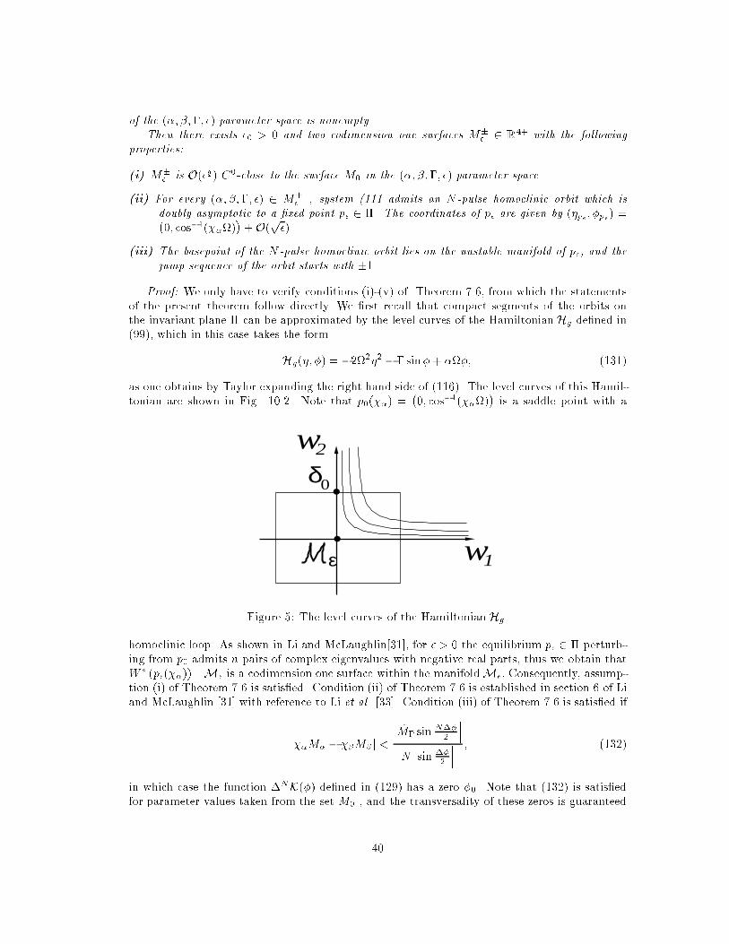
of the (�; �;�; �) parameter space is nonempty.Then there exists �0 > 0 and two codimension one surfaces M�� 2 R4+ with the followingproperties:(i) M�� is O(�q) C0-close to the surface M0 in the (�; �;�; �) parameter space.(ii) For every (�; �;�; �) 2 M�� , system (111 admits an N -pulse homoclinic orbit which isdoubly asymptotic to a �xed point p� 2 �. The coordinates of p� are given by (�p�; �p�) =�0; cos�1(��)�+ O(p�).(iii) The basepoint of the N -pulse homoclinic orbit lies on the unstable manifold of p�, and thejump sequence of the orbit starts with �1.Proof: We only have to verify conditions (i)-(v) of Theorem 7.6, from which the statementsof the present theorem follow directly. We �rst recall that compact segments of the orbits onthe invariant plane � can be approximated by the level curves of the Hamiltonian Hg de�ned in(99), which in this case takes the formHg(�; �) = �22�2 � � sin�+ ��; (131)as one obtains by Taylor expanding the right hand side of (116). The level curves of this Hamil-tonian are shown in Fig. 10.2. Note that p0(��) = �0; cos�1(��)� is a saddle point with aε w1

w2

0δFigure 5: The level curves of the Hamiltonian Hg .homoclinic loop. As shown in Li and McLaughlin[31], for � > 0 the equilibrium p� 2 � perturb-ing from p0 admits n pairs of complex eigenvalues with negative real parts, thus we obtain thatW s (p�(��))\M� is a codimension one surface within the manifoldM�: Consequently, assump-tion (i) of Theorem 7.6 is satis�ed. Condition (ii) of Theorem 7.6 is established in section 6 of Liand McLaughlin [31] with reference to Li et al. [33]. Condition (iii) of Theorem 7.6 is satis�ed ifj��M� � ��M� j < ���M̂� sin N��2 ���N ���sin ��2 ��� ; (132)in which case the function �NK(�) de�ned in (129) has a zero �0. Note that (132) is satis�edfor parameter values taken from the set M0 , and the transversality of these zeros is guaranteed40

by condition (124). Therefore, assumption (iii) of Theorem 7.6 is satis�ed. The validity ofassumption (iv) can be seen from the phase portrait in Fig. 10.2.To prove the theorem, it remains to verify condition (v) of Theorem 7.6. This can be done byadapting the distance measurement used in McLaughlin et al. [34] and Li and McLaughlin [31]as follows. The point p̂ = (0; 0; �0(��); �0(��) + N��) lies on the stable manifold of p0 if thevalue of HamiltonianHg at p̂ is the same as at some other point of the homoclinic loop attachedto p0. In particular, it su�ces to require thatHg(�0(��); �0(��)) = Hg(�0(��); �0(��) +N��):From (131) we obtain that this last equation can be written in the form2� cos��0(��) + N��2 � sin ��2 � �N�� = 0: (133)Using the expression of �NK(�) and the fact that �0(��) is a zero of �NK(�); we can rewrite(133) as �� � ��M� M� � M̂��� sin N��22 sin2 ��2 ! = 0:The transverse crossing of the unstable manifold of p0 by the point p̂ is equivalent to the left handside of this equation admitting a nonzero derivative with respect to, e.g., the parameter �� at asolution ��(�;�;; N ). Since the equation is linear in ��; this transversality condition clearlyholds, thus condition (v) of Theorem 7.6 is satis�ed. This concludes the proof of the theorem. �We remark that Li and McLaughlin [31] showed that the set M0 de�ned in the statementof the above theorem is nonempty for K > 7 and for N = 1 (i.e., for single-pulse homoclinicorbits). We also note that the multi-pulse homoclinic orbits obtained from the theorem have thesame asymptotic behavior as the single-pulse homoclinic orbits, hence the construction of chaoticinvariant sets in their vicinities can be directly adapted from Li and Wiggins [32].11 ConclusionsIn this paper we gave a general criterion for the existence of nontrivial homoclinic orbits in alarge class of near-integrable, multi-dimensional systems that usually arise as modal truncationsor discretizations of partial di�erential equations. The homoclinic orbits we constructed makerepeated departures from, and returns to, a codimension two invariant manifold which carriessolutions with a slow and a fast time scale. The shape of the pulses (i.e., excursions of thehomoclinic orbits) can be descried by a sequence of +1s and �1s which we compute explicitly.Our results generalize the energy-phase method in Haller [16] and Haller and Wiggins [19] toarbitrarily high (but �nite) dimensional systems.We remark that if the perturbation in equation (1) is purely Hamiltonian (i.e., g � 0), thenthe multi-pulse orbits generically undergo a sequence of universal bifurcations as the parametersof the system are varied. Such a bifurcation has been �rst described in an example in Haller[15] and then were shown to be generic near double resonances of near-integrable Hamiltoniansystems in Haller [15]. Since for purely Hamiltonian perturbations, the energy-di�erence function�NH obtained in this paper is the same as in [15], the same universality holds for the bifurcationsof multi-pulse orbits in system (1).As an application of our results, we showed that the discretized, perturbed NLS equationadmits multi-pulse solutions homoclinic to its center manifold. In fact, the pulse number of these41

orbits can be arbitrarily high if the dissipative and forcing terms are small enough. Statement(ii) of the Theorem 10.1 also shows that N -pulse orbits with quite di�erent shapes will coexist.Furthermore, statement (iii) describes how the unstable manifold of the plane � disintegratesthrough multi-pulse jumping into components which display completely di�erent jumping behav-iors. Since the multi-pulse orbits spend a time of order O (log1=p�) (as opposed to O(1=p�) asin Kaper and Kova�ci�c [26]) in the neighborhood of the manifoldM�, they have observable openneighborhoods in which solutions exhibit the same type of jumping behavior for �nite times.Given the close coexistence of multi-pulse orbit families with di�erent jump sequences, one ex-pects to see a transient type of chaotic dynamics in numerical simulations. This agrees well withthe irregular jumping behavior observed by Bishop et al. [5],[6] for � = 0.Finally, we also considered the discretized NLS equation with a mode-dependent dampingterm (� 6= 0). Making use of the calculations of Li and McLaughlin [31], we showed the existenceof multi-pulse Silnikov-type homoclinic orbits for a codimension one set of parameter values.This provides a signi�cant extension of the set of parameter values for which the discretized NLSequation admits chaotic invariant sets in its phase space.AcknowledgmentI am grateful to Dave McLaughlin for several useful discussions on the subject of this paperand for making ref. [31] available to me before its publication.References[1] Ablowitz, M.J. and Ladik, J.F., Nonlinear di�erential-di�erence equations and Fourier anal-ysis, J. Math. Phys. 17 (1976) 1011-1018.[2] Ablowitz, M.J. and Herbst, B.M., On homoclinic structures and numerically induced chaosfor the nonlinear Schr�odinger equation, SIAM J. Appl. Math. 50 (1990) 339-351.[3] Arnold, V.I.,Mathematical Methods of Classical Mechanics, (2nd. ed.) Springer-Verlag, NewYork (1978).[4] Becker, J. and Miles, J. W., Parametric excitation of an internally resonant double pendu-lum, II., Z. Angew. Math. Phys. 37 (1986) 641-650.[5] Bishop A.R., Forest, M.G., McLaughlin, D.W., and Overman, E.A., A modal representationof chaotic attractors for the driven, damped pendulum chain, Phys. Lett. A 144 (1990)17-25.[6] Bishop, A.R., Flesch, R., Forest, M.G., McLaughlin, D.W., and Overman, E.A., Correlationsbetween chaos in a perturbed Sine-Gordon equation and a truncated model system, SIAMJ. Math. Anal. 21 (1990) 1511-1536.[7] Bogolyubov, N. N. and Prikarpatskii, A. K., The inverse periodic problem for a discreteapproximation of the nonlinear Schr�odinger equation, Sov. Phys. Dokl. 27/2 (1982) 113-116.[8] Ercolani, N.M., Forest, M.G., and McLaughlin, D.W., Geometry of the modulational in-stability, Part III: Homoclinic Orbits for the periodic sine-Gordon equation, Physica D 43(1990) 349-384. 42

[9] Ercolani, N.M. and McLaughlin, D.W., Towards a topological classi�cation of integrablePDE's, in The Geometry of Hamiltonian Systems, Springer-Verlag, New York (1991).[10] Feng, Z.C. and Sethna, P.R., Global bifurcations in the motion of parametrically excitedthin plates, Nonlinear Dynamics 4 (1993) 398-408.[11] Feng, Z.C. and Wiggins, S., On the existence of chaos in a class of two-degree-of-freedom,damped, strongly parametrically forced mechanical systems with broken O(2) symmetry,ZAMP 44 (1993) 201-248.[12] Feng, Z.C. and Leal, Symmetries in the amplitude equations of an inextensional beam withinternal resonance, J. Appl. Mech. 62/1 (1995) 235-238.[13] Fenichel, N., Persistence and smoothness of invariant manifolds for ows, Ind. Univ. Math.J. 21 (1971) 193-225.[14] Fenichel, N., Geometric singular perturbation theory for ordinary di�erential equations, J.Di�. Eqs. 31 (1979) 53-98.[15] Haller, G., Multi-pulse Homoclinic Phenomena is Resonant Hamiltonian Systems, PhD.Thesis, Caltech (1993).[16] Haller, G. and Wiggins, S., Orbits homoclinic to resonances: the Hamiltonian case, PhysicaD 66 (1993) 298-346.[17] Haller, G. and Wiggins, S., Whiskered tori and chaos in resonant Hamiltonian normal forms,in Normal Forms and Homoclinic Chaos, Fields Institute Communications (1995) (in press).[18] Haller, G. and Wiggins, S., N-pulse homoclinic orbits in perturbations of resonant Hamilto-nian systems, Arch. Rat. Mech. and Anal. 130 (1995) 25-101.[19] Haller, G. and Wiggins, S., Multi-pulse jumping orbits and homoclinic trees in a modaltruncation of the damped, forced nonlinear Schr�odinger equation, Physica D 85 (1995) 311-347.[20] Haller, G., Universal homoclinic bifurcations and chaos near double resonances, J. Stat.Phys. (1997) 1011-1051.[21] Haller, G.,Homoclinic Chaos in Resonant Dynamical Systems, Springer-Verlag (in prepara-tion).[22] Holmes, P., Chaotic motion in a weakly nonlinear model for surface waves, J. Fluid. Mech.162 (1986) 365-388.[23] Jones, C.K.R.T. and Kopell, N., Tracking invariant manifolds with di�erential forms insingularly perturbed systems, J. Di�. Eqs. 108 (1994) 64-88.[24] Jones, C.K.R.T., Kaper, J., and Kopell, N., Tracking invariantmanifolds up to exponentiallysmall errors, SIAM J. Math. Anal.(1995) (to appear).[25] Kambe, T. and Umeki, M., Nonlinear dynamics of two-mode interactions in parametricexcitation of surface waves, J. Fluid. Mech. 212 (1990) 373-393.[26] Kaper, T.J. and Kova�ci�c, G., Multiple-pulse homoclinic orbits near resonance bands, preprint(1993). 43

[27] Kova�ci�c, G. and Wiggins, S., Orbits homoclinic to resonances, with an application to chaosin the damped and forced Sine-Gordon equation, Physica D 57 (1992) pp. 185-225.[28] Kova�ci�c, G. and Wettergren, T.A., Homoclinic orbits in the dynamics of resonantly drivencoupled pendula, preprint (1994).[29] Li, Y., B�acklund transformations and homoclinic structures for the integrable discretizationof the NLS equation, Phys. Lett. A 163 (1992) 181-187.[30] Li, Y. and McLaughlin, D.W., Morse and Melnikov functions for NLS PDE's, Comm. Math.Phys. 162 (1994) pp. 175-214.[31] Li, Y. and McLaughlin, D.W., Homoclinic orbits and chaos in discretized perturbed NLSsystems, Part I.: Homoclinic orbits, J. Nonlin. Sci. 7 (1997) 211-269.[32] Li, Y. and Wiggins, S., Homoclinic orbits and chaos in discretized perturbed NLS systems,Part II.: Symbolic dynamics,J. Nonlin. Sci. 7 (1997) 315-370.[33] Li, Y., McLaughlin, D., Shatah, J., and Wiggins, S., Persistent homoclinic orbits for aperturbed nonlinear Schr�odinger equation,, Comm. Pure Appl. Math 49 (1996) 1175-1255.[34] McLaughlin, D., Overman, E.A.II., Wiggins S., and Xiong, C., Homoclinic orbits in a fourdimensional model of a perturbed NLS equation: a geometric singular perturbation study,in Dynamics Reported 5, Springer-Verlag, Berlin (1993).[35] Miles, J. W., Parametric excitation of an internally resonant double pendulum, Z. Angew.Math. Phys. 36 (1985) 337-345.[36] Miller, P. D., Ercolani, N.M., Krichever, I.M., and Levermore, C.D., Finite genus solutionsto the Ablowitz-Ladik equations Comm. Pure Appl. Math. (1995) (to appear).[37] Nayfeh, A.H. & Pai, P.F., Non-linear, non-planar parametric responses of an inextensionalbeam, Int. J. Non-lin. Mech. 24 (1989) 139-158.[38] Tien, W.M. and Namamchchivaya,N.S., Nonlinear dynamics of a shallow arch under periodicexcitation II: 1: 1 internal resonance, Int. J. Non-Lin. Mech. 29(3) (1994) pp. 367-386.[39] Tin, S. K., On the Dynamics of Tangent Spaces near a Normally Hyperboloc InvariantManifold, Ph.D. Thesis, Brown University (1994).[40] Yang, X.L. and Sethna, P.R., Non-linear phenomena in forced vibrations of a nearly squareplate: antisymmetric case, J. Sound and Vib. 155 (1992) pp. 413-441.[41] Zakharov, V.E. and Shabat, A.B., Exact theory of two dimensional self-focusing and onedimensional self-modulation of waves in nonlinear media, Sov. Phys. JETP 34 (1972) pp.62-69.44

Figure captions:Figure 1: The chain of heteroclinic orbits xi(t).Figure 2: 3-pulse homoclinic orbit to the manifoldM� with jump sequence j = f+1;�1;+1gand with basepoint b�.Figure 3: The de�nition of the vector n(p+) in two di�erent cases.Figure 4: The geometry of the proof of Theorem 7.6.Figure 5: The level curves of the Hamiltonian Hg.

45