Multi-body Dynamics Simulation and

Analysis of Wave-adaptive Modular Vessels

John D. Fratello

Thesis submitted to the faculty of Virginia Polytechnic Institute and

State University in partial fulfillment for the degree of

Master of Science

In

Mechanical Engineering

Mehdi Ahmadian, Chair

Leigh S. McCue-Weil

Saied Taheri

April 29, 2011

Blacksburg, Virginia

Keywords: Catamaran seakeeping, suspension dynamics,

shock mitigation, multi-body dynamics simulation

Copyright © 2011, John D. Fratello

Multi-body Dynamics Simulation and

Analysis of Wave-adaptive Modular Vessels

John D. Fratello

Abstract

Catamarans provide vast deck space, high thrust efficiency, and excellent transverse stability,

however, in rough conditions they can be susceptible to deck slamming from head seas or bow

diving in following seas and a pitch-roll coupling effect that can lead to uncomfortable

corkscrew motion under bow-quartering seas. A new class of catamaran called Wave-Adaptive

Modular Vessels (WAM-V™) aims to help mitigate oceanic input from the cabin by allowing

for the relative motion of components not common to classic catamaran design. This thesis

presents a set of multi-body dynamics simulation models created for two active WAM-Vs™

along with analysis on their suspension characteristics. Both models provide conclusive and

realistic results, with the final model being validated against on-water testing data from a 12-ft

unmanned prototype WAM-V™.

The first of these simulations serves primarily as a tool to evaluate WAM-V™ response

characteristics with respect to a variety of parametric variations. The modeling environment is

highlighted along with details of the parametric simulation and how it was created. The results

fall in line with our expectations and are presented along with analysis of the sensitivity of each

parameter at three longitudinal locations. The final simulation attempts to model the response of

a 12-ft unmanned surface vessel (USV) prototype of the WAM-V™ configuration. Testing data

is collected, processed, and applied to the model for validation of its prediction accuracy. The

results of the sea tests indicate that the simulation model performs well in predicting USV

motions at sea. Future considerations for testing WAM-Vs™ can include changes in suspension

and mass parameters as well as limiting particular degrees-of-freedom by making their joints

rigid.

iii

Contents

List of Tables ................................................................................................................................................ v

List of Figures .............................................................................................................................................. vi

Chapter 1 ....................................................................................................................................................... 1

Introduction ................................................................................................................................................... 1

1.1 A Broad Overview of Catamaran Characteristics ......................................................................... 2

1.2 Wave-Adaptive Modular Vessel (WAM-V™) ............................................................................. 4

1.3 Research Objectives ...................................................................................................................... 6

1.4 Approach ....................................................................................................................................... 6

1.5 Outline........................................................................................................................................... 7

Chapter 2 ....................................................................................................................................................... 8

Technical Background and Literature Review .............................................................................................. 8

2.1 Review of Common Displacement Hull Forms ............................................................................ 8

2.2 Introduction to Wave Adaptive Modular Vessels ....................................................................... 10

Chapter 3 ..................................................................................................................................................... 12

Proteus Modeling ........................................................................................................................................ 12

3.1 Proteus Details ............................................................................................................................ 12

3.2 Modeling Environment – SimMechanics ................................................................................... 13

3.3 Proteus Modeling ........................................................................................................................ 16

3.4 Parametric Analysis .................................................................................................................... 22

Chapter 4 ..................................................................................................................................................... 32

Unmanned Surface Vessel Characteristics ................................................................................................. 32

4.1 USV Design Overview................................................................................................................ 32

4.2 Physical Property Measurement and Static Testing .................................................................... 35

4.3 USV Multi-Body Dynamic Model Development ....................................................................... 35

iv

4.4 Spring and Damper Modeling ..................................................................................................... 37

Chapter 5 ..................................................................................................................................................... 41

Unmanned Surface Vessel Dynamic Testing .............................................................................................. 41

5.1 Instrumentation ........................................................................................................................... 41

5.2 Test Setup.................................................................................................................................... 46

5.3 On-water Testing ........................................................................................................................ 48

5.4 Model Input Pre-processing ........................................................................................................ 49

5.4.1 Noise Reduction ...................................................................................................................... 50

5.4.2 Acceleration Integration .......................................................................................................... 54

5.5 Single Degree of Freedom Modeling and Results ...................................................................... 59

5.6 Multi-Body Dynamic Simulation Results and Validation .......................................................... 62

Chapter 6 ..................................................................................................................................................... 69

Concluding Remarks ................................................................................................................................... 69

6.1 Summary and Discussion ............................................................................................................ 69

6.1.1 Parametric Analysis of Proteus ............................................................................................... 69

6.1.2 USV Modeling & Validation .................................................................................................. 71

6.2 Recommendations ....................................................................................................................... 72

Appendices .................................................................................................................................................. 74

A. Acceleration Integration – Omega Arithmetic............................................................................ 74

B. USV Single-DOF Model ............................................................................................................ 76

References ................................................................................................................................................... 78

v

List of Tables

Table 3-1. Description of Modes of Input Motion to Proteus...................................................... 24

Table 3-2. Percent Variation of Parameters ................................................................................. 26

Table 3-3. Example of Sensitivity Results ................................................................................... 26

Table 5-1. Wave Direction Relative to USV and Vessel Heading per Leg ................................. 47

Table 5-2. Summary of Events Completed During Testing ........................................................ 49

Table 5-3. Integration Filter Calibration Test Procedure ............................................................. 58

Table 5-4. Linear Damping Coefficients Tested for Assumption Validation .............................. 63

Table 6-1. Summary of Parametric Analysis Results .................................................................. 70

vi

List of Figures

Figure 1.1. The sustention triangle shows that the primary lifting forces on vessels can be split

into three primary categories: buoyancy, dynamic lift and powered lift [5]. ................................. 1

Figure 1.2. Fuel consumption predictions for comparable catamaran and monohull at full and

light displacement [12]. .................................................................................................................. 2

Figure 1.3. The Proteus is a WAM-V™ concept of catamaran which utilizes springs and a ball

joint to help mitigate oceanic inputs to the cabin and improve passenger comfort. ....................... 4

Figure 1.4. The engine pods of Proteus are attached to the pontoons with a pivot joint that allows

the pod to rotate about the lateral axis freely with respect to the pontoon. .................................... 5

Figure 2.1. Example of a SWATH hull form. The water line sits just above the lower hull at

some point along the strut [11]. ...................................................................................................... 9

Figure 2.2. The springs positioned above each pontoon/arch attachment provide for mitigation

of the heaving and pitching motions inherent to catamarans. ....................................................... 10

Figure 3.1. A simple grounded mass-spring-damper system. ...................................................... 13

Figure 3.2. Representation of the MATLAB code used to solve the MSD system. .................... 14

Figure 3.3. Representation of the Simulink code used to solve the MSD system. ...................... 15

Figure 3.4. The MSD system as depicted using SimMechanics. Notice the physical nature of the

modeling environment. ................................................................................................................. 16

Figure 3.5. A stock car rests atop the input pads at the shaker rig located at VIPER in Danville,

VA. ................................................................................................................................................ 17

Figure 3.6. The under-workings of a shaker rig involve very large numerically controlled

hydraulic pistons used to excite the vehicle’s suspension. ........................................................... 17

vii

Figure 3.7. Leaf springs were replaced with cylinders to ease the process of dynamic force

application within the SimMechanics environment. Top: front suspension / Bottom: rear

suspension. .................................................................................................................................... 19

Figure 3.8. The SimMechanics model was organized to be visually comparable to the Proteus

top-view appearance. .................................................................................................................... 20

Figure 3.9. The suspension bases were only restricted from pitching rotations and were driven

with vertical translations. Here the capital letters P and R stand prismatic and rotational axes,

respectively. .................................................................................................................................. 21

Figure 3.10. The signal used to drive the parametric model removed as many discontinuities as

possible. ........................................................................................................................................ 24

Figure 3.11. Variance in output sensitivity percentage from front to rear of the chassis from

heave input. ................................................................................................................................... 28

Figure 3.12. Variances in output sensitivity from front to rear of the chassis from pitch input. . 30

Figure 4.1. The USV retains representative architecture to Proteus with the obvious addition of

rigid skis between the front suspension and rear arch attachment. ............................................... 33

Figure 4.2. The rear joint of the USV utilizes a combined ball and shaft to allow it freedom to

rotate about the transverse and vertical axes only. ....................................................................... 34

Figure 4.3. A spherical joint was utilized to attach the front arch and suspension and to allow for

properly constrained motion of the pontoons relative to one another. ......................................... 34

Figure 4.4. The USV CAD model is much simpler in architecture than the Proteus model. ...... 36

Figure 4.5. This graph depicts the averaged left and right side raw spring force data. ............... 37

Figure 4.6. Non-linearities in the suspension stiffness arise from two major areas which are

called out in this depiction of the left from suspension system on the USV. ............................... 38

Figure 4.7. This figure represents the final single spring force vs. displacement curve. The blue

points represent measured data and the red points at either end represent estimated data. .......... 39

viii

Figure 4.8. The USV response to 2 inches of initial compression exhibits the low damping ratio.

....................................................................................................................................................... 40

Figure 5.1. The CompactRIO is completely reconfigurable, allowing for comprehensive

customization. ............................................................................................................................... 42

Figure 5.2. The battery and CompactRIO were situated within a water resistant box. Twelve

waterproof connectors and an Ethernet port were also installed. ................................................. 42

Figure 5.3. Accelerometers were mounted close to each arch attachment atop the rigid skis. .... 43

Figure 5.4. Linear potentiometers were used to measure spring deflection while testing. .......... 44

Figure 5.5. A string pot was installed using a custom mount to retain linearity of the

measurement for both directions of motion. ................................................................................. 45

Figure 5.6. The tri-axial cabin accelerometer was mounted directly to the base plate within the

water resistant box. ....................................................................................................................... 46

Figure 5.7. A star pattern was utilized to ensure that data was taken with waves striking the

vessel at each of five important directions. ................................................................................... 47

Figure 5.8. This visual example of the FFT averaging scheme utilizes three decimated time

series’ to collate into the final frequency spectrum. ..................................................................... 51

Figure 5.9. A portion of pontoon accelerometer data showing the engine both off and on. ....... 52

Figure 5.10. The dominant frequencies of the engine noise can clearly be identified. ............... 52

Figure 5.11. The Butterworth lowpass filter clearly eliminates engine noise with little trouble. 54

Figure 5.12. Discretization of continuous time-series signals leads to errors when a trapezoidal

integration scheme is applied. ....................................................................................................... 55

Figure 5.13. Integration error can stem from things such as a DC offset or other dynamic

variations in central tendency. ...................................................................................................... 56

ix

Figure 5.14. A damper dynamometer was outfitted with sensors to gather calibration data for the

integration filter. ........................................................................................................................... 58

Figure 5.15. A 1-DOF model was developed to predict USV suspension response frequencies. 59

Figure 5.16. The spring force vs. displacement curve was simplified using 4 linear curve fits.

The lower numbers in the figure represent statistical displacement percentiles from testing. ..... 60

Figure 5.17. The frequency response of the linear spring potentiometer showcases both the input

and suspension response frequencies. ........................................................................................... 61

Figure 5.18. Two seconds of linear spring potentiometer displacement data displaying both the

impact and suspension response frequencies. ............................................................................... 62

Figure 5.19. As the data from Figure 5.18 is manually analyzed, it reveals the same frequencies

found from the Fourier analysis. ................................................................................................... 62

Figure 5.20. Variation of right front spring displacement response due to damping coefficient. 64

Figure 5.21. Variation of right front spring velocity response due to damping coefficient. ....... 65

Figure 5.22. Variation in center of gravity vertical acceleration response due to damping

coefficient. .................................................................................................................................... 66

Figure 5.23. In the time domain the USV simulation appears to very accurately represent the

realistic testing measurements. ..................................................................................................... 68

Figure B-1. The USV was modeled as a pinned-and-cantilevered beam with a spring opposite

the pin…………………………………………………………………………………………….76

1

Chapter 1

Introduction

The purpose of this chapter is to familiarize the reader with various types of marine vessels with

a special emphasis being put on the advantages and disadvantages of catamaran designs. The

fundamental lifting forces acting upon a ship can be split into three categories as can be seen in

the Sustention Triangle of Figure 1.1: displacement buoyancy, dynamic lift and powered lift.

This scope of this discussion will be limited to vessels relying solely on water displacement

buoyancy, which will be defined as craft whose lift comes as a result of static buoyancy and does

not vary with increasing velocity.

Figure 1.1. The sustention triangle shows that the primary lifting forces on vessels can be split into three

primary categories: buoyancy, dynamic lift and powered lift. Used under Fair Use Guidelines, [5].

These displacement-type vessels can be split into two major categories: those with a

single hull and those with multiple hulls. Catamarans are defined as two-hulled vessels whose

primary flotation source rests at the water line. This concept can be extended to include various

numbers of hulls including trimarans (three hulls) and pentamarans (five hulls), which begin to

bridge the gap between single-hulled vessels and true catamarans in terms of lateral stability [4].

2

1.1 A Broad Overview of Catamaran Characteristics

Catamarans have several inherent advantages over standard monohull designs; however their

application in seaways can be limited. Due to their geometry, catamarans can have much larger

deck area and enjoy greater roll stability than a comparative displacement monohull vessel [5, 7,

8, 11, 14]. A properly designed catamaran can produce similar roll accelerations to a monohull

[7] with rolling amplitudes 2.5 times smaller [10]. Catamarans have larger wetted area than

comparable monohulls, which will lead to increased parasitic drag, but they generally require

less total propulsive power due to their high aspect ratio hulls that can reduce wave resistance

and therefore fuel consumption [5, 7, 13]. This effect is especially pronounced at higher speeds

where wave resistance makes a greater impact as can be seen in Figure 1.2 below [12]. If

equipped with individually-operated propulsors for each pontoon the catamaran can benefit from

increased maneuverability via differential thrust [12] and a fault tolerance should an engine fail

while underway.

Figure 1.2. Fuel consumption predictions for comparable catamaran and monohull at full and light

displacement. Used under Fair Use Guidelines, [12].

Catamarans do, however, come with a slight set of drawbacks as well. Baitis, et al. [1]

concluded that a catamaran produced the worst seakeeping results as compared to three

3

monohulls and two SWATHs all designed for the same mission. Another consideration of great

importance is their susceptibility to wet deck slamming in rough seas which can cause passenger

discomfort or structural damage to the vessel [3, 5, 8, 9, 10, 11, 14]. Varyani, et al. [14] created

a three-dimensional computational model to analyze the loads for a slamming incident in a

catamaran drop test. They concluded that the narrow hull forms resulted in small magnitude

loads while those encountered by the cross structure from its impact with the water can be quite

large. Bonafoux, et al. [3] found that slam occurrences begin as significant wave height

approaches the wet deck clearance, but a decrease from full speed actually increases the

occurrence of slamming events. Fang and Chan [9] stated that catamarans can also be prone to

bow diving in strong following seas.

Several studies have been performed to analyze the motion sickness incidence (MSI) or

various vessels. Bonafoux, et al. [3] compared the motions of a monohull, catamaran, and

pentamarans all of identical payload capacity. Their results indicate that the catamaran has the

worst MSI in head and bow quartering seas, but performs the best of the three in beam seas.

Davis and Holloway [6] modeled the response of several catamarans, trimarans, SWATHs, and

monohulls using time domain strip theory. They concluded that in high seas the catamarans and

SWATHs performed about the same with an approximate MSI of 50% to 70% while the

monohulls and trimarans showed much better results with an MSI range of 40% to 50%. At

lower significant wave height the SWATHs produced the least MSI at 0% to 5%, the monohulls

and trimarans 5% to 10%, and the catamarans 5% to 15%. Turan, et al. [13] did work to produce

a better model to estimate MSI from data recorded on vessels, which found that lateral

acceleration plays an important role in the generation of sea sickness. During their tests they

also discovered that lateral and vertical RMS accelerations at various locations on the vessel are

equivalent for the catamaran, while the lateral acceleration of a monohull is approximately half

that of the vertical acceleration.

Due to the high transverse stability of catamarans they can have similar natural roll and

pitch frequencies. When encountering bow quartering seas, an out-of-phase dynamic coupling

can occur in pitch and roll creating a corkscrew motion [5, 10, 12]. Another downside to this

high stability is that at large roll angles the righting moment becomes very strong, which can

create elevated roll accelerations [10].

4

1.2 Wave-Adaptive Modular Vessel (WAM-V™)

Several designs have been developed to help mitigate oceanic input into catamarans.

Some of the more common methods involve the use of subsurface hydrofoils or stabilizing fins

to add vertical damping to the system and alleviate some of the buoyant forces at work in high

seas. Another concept which has been developed is the wave-adaptive modular vessel (WAM-

V™), which retains the inherent advantages in speed and range afforded to a catamaran while

supplying methods to help alleviate oceanic inputs and improve passenger comfort. This novel

concept combines two innovative ideas on catamaran design. The first is the use of springs to

attach the pontoons to the superstructure. This provides a flexible structure which can store and

dissipate energy during the motion caused by waves. The second design innovation is the

installation of a spherical joint between the main cabin structure and the front arch. This allows

the front arch to rotate freely with respect to the cabin in turn providing independent motion of

the front of either pontoon with respect to the other. Figure 1.3 depicts a 100-ft prototype

WAM-V™ named Proteus.

Figure 1.3. The Proteus is a WAM-V™ concept of catamaran which utilizes springs and a ball joint to

help mitigate oceanic inputs to the cabin and improve passenger comfort. Photo by author, 2011.

5

These advancements may help in terms of passenger comfort, but the architecture of

WAM-Vs™ still leaves them susceptible to several potential problems. Proteus is propelled

from engine pods mounted to the aft of each pontoon. Pivot joints attach the pods to the

pontoons and allow for the engine pod to pitch freely with respect to the pontoons as can be seen

in Figure 1.4. The goal of this design is to allow the propellers to stay in contact with the water

as the aft of the vessel crests waves. As the engine pod pitches, however, the thrust vector

changes direction, which produces oscillating surge accelerations felt at the cabin. This

propulsion layout could also make it difficult to utilize water jets, which are much more efficient

at high speed. The linear velocity at the tips of propellers can cause cavitation at speeds

exceeding 30 knots whereas the impellers of a water jet propulsion system remain effective [10].

Figure 1.4. The engine pods of Proteus are attached to the pontoons with a pivot joint that allows the pod

to rotate about the lateral axis freely with respect to the pontoon. Photo by author, 2011.

Another potential downfall of the WAM-V™ concept stems from the utilization of the

suspension itself. As the springs compress, the cross structure clearance to the water line reduces,

which could induce an increased number of slamming events to the lower cabin structure in high

seas. However, these impacts will likely not be of the order felt in a standard catamaran with an

enclosed center tunnel because the water will have an escape route once it strikes the cabin and

the pressure spike should dissipate quickly.

Engine Pod Pivot Joint

6

1.3 Research Objectives

The primary objectives of this study are:

1) create a dynamic simulation model and perform analysis on the 100-ft prototype

Proteus’ suspension characteristics,

2) perform similar modeling on 12-ft unmanned prototype WAM-V™, instrument and

perform testing on actual vessel, and validate test data to simulation,

3) characterize basic response parameters of the 12-ft unmanned surface vessel (USV)

using simple models and validate with testing data, and

4) provide recommendations for future studies on WAM-Vs™.

1.4 Approach

During the course of this research, two main dynamic simulation models were created. Both

models captured the vertical dynamic motion of the cabin with respect to pontoon action. The

first model was kinematically accurate to the Proteus and was used to characterize parametric

sensitivities on that particular vessel. The second was a simpler model used to mimic the

prevalent characteristics of the 12-ft USV and was employed as a validation tool for the usage of

dynamic simulations on these hull forms in replacement of testing. To defend these validating

arguments the USV was carefully instrumented and tested on open water. A simple model was

used to compare natural frequency estimation of the USV suspension with frequency response

data recorded while testing. Based upon the results presented from these analyses, further

modeling and prediction recommendations are made for these vessels.

7

1.5 Outline

Chapter 2 briefly outlines the technical background of various displacement hull forms and their

seakeeping characteristics, as well as a primer on essential WAM-V™ architecture. Chapter 3

covers the principle characteristics of Proteus as well as the dynamic simulation development

and results from a parametric analysis of its suspension. Chapter 4 details the primary variations

of the USV from Proteus as well as the dynamic model created to represent it and the physical

measurements made to ensure its accuracy. The USV instrumentation, testing, data pre-

processing and validation discussion are presented in Chapter 5. Chapter 6 summarizes the work

that was completed and provides recommendations for future prediction algorithms of WAM-

V™ dynamics.

8

Chapter 2

Technical Background and Literature Review

The purpose of this chapter is to introduce the reader to the advantages and disadvantages of

several types of marine displacement hull forms. A discussion is presented comparing the

benefits and downfalls of monohulls, catamarans, trimarans, pentamarans and SWATH vessels.

Specific emphasis is placed on the trade-offs between deck space, stability, speed, fuel efficiency

(range) and seakeeping. Lastly, the primary goals of wave adaptive modular vessels are

presented along with the variations from classic catamaran design required to create them.

2.1 Review of Common Displacement Hull Forms

The majority of marine vessels in use today rely primarily upon the lift created by the

displacement of water to stay afloat. As discussed previously, multihulled ships have several

distinct advantages over monohulls including greater deck area, excellent transverse stability,

and less required power for a given speed. By varying hull shape and number, multihulls can

take various forms that produce vastly different characteristics. Catamarans are twin-hulled

vessels whose primary buoyant structure rests at the water line. A broad discussion of the

advantages, disadvantages, and characteristics of catamarans was presented in section 1.1. The

small-waterplane-area twin-hull (SWATH) utilizes two fully submerged submarine-like hulls

attached to the superstructure with high aspect ratio streamlined struts as can be seen in Figure

2.1 [11]. This reduces submerging stiffness because the struts at the water line have very low

volumetric displacement per vertical motion, thereby reducing oceanic inputs to the cabin.

Trimarans and pentamarans are three- and five-hulled vessels, respectively, and they are thought

to have an intermediate transverse stability between monohulls and catamarans [4].

9

Figure 2.1. Example of a SWATH hull form. The water line sits just above the lower hull at some point

along the strut. Used under Fair Use Guidelines, [11].

The high stability offered to catamarans can sometimes become problematic at high sea

states because the righting forces on the vessel are very strong. SWATHs retain many of the

advantages of catamarans while bettering passenger comfort, however, this only plays a

significant role at higher sea states [6]. SWATHs suffer from much higher levels of resistance

than a standard catamaran due to increased underwater surface area. This also results in top

speeds much slower than a comparable catamaran [10]. By the nature of their architecture and

construction, SWATH vessels will run a deeper draft and cost more to manufacture than a classic

catamaran [10].

Trimarans and pentamarans have greater transverse stability than comparable monohulls.

To attain this, lateral outriggers are mounted aside a primary central hull form. The increased

resistance can be tuned to reduce wave resistance with proper lateral and longitudinal outrigger

offset or frictional resistance by utilizing shallow outrigger hulls to decrease wetted area. When

shallow outriggers are used, nonlinearity can arise in the roll stabilizing moment response

because the unladen outriggers emerge from the surface at very moderate roll angles. This

discontinuity produces two attractors at a single forcing frequency. When excited with this

natural roll period, attractor jumping can be witnessed between large amplitude resonance and

low amplitude anti-resonance depending on the initial conditions [4]. Another downside to

running shallow draft outriggers on these vessels is that propulsion most likely will come from a

single source on the central hull, which limits their maneuverability with respect to the

differential power steering capabilities of catamarans. Both of these issues can be mitigated by

using much deeper outrigger hull forms, but that comes at the expense of increased resistance.

Bonafoux, et al. [3] studied the seakeeping characteristics of a monohull, catamaran, and

pentamaran in various wave incident directions. They found that the pentamaran had the least

10

motion sickness incidence in head seas, equivalent to the monohull and better than the catamaran

in bow quartering seas, and the worst MSI of the three in beam seas.

2.2 Introduction to Wave Adaptive Modular Vessels

The concept of a wave adaptive modular vessel (WAM-V™) came about in an effort to reap the

many advantages inherent to catamarans while mitigating many of the unwanted responses

characteristics also common to those designs. The most visually prevalent design concept of

these vessels is the suspension system installed between each arch/pontoon attachment. Figure

2.2 depicts the right front suspension of the 100-ft WAM-V™ Proteus, which was illustrated in

Figure 1.3. The suspensions act to store and dissipate the pitch and heave energy produced at the

pontoons, thus reducing those motions as they are felt at the cabin.

Figure 2.2. The springs positioned above each pontoon/arch attachment provide for mitigation of the

heaving and pitching motions inherent to catamarans. Photo by author, 2011.

In an effort to reduce the common coupling between pitch and roll exhibited in catamaran

seakeeping and to allow the vessel to easily absorb quartering waves (those which produce

pitching and rolling motions simultaneously) an innovative approach was taken to WAM-V™

superstructure design. Rather than forcing the pontoons to remain parallel with rigid attachments

front-to-back and side-to-side, a spherical joint was installed between the main cabin and front

11

arch. This allows the front arch to rotate freely (primarily about a longitudinal axis passing

through the joint) with respect to the cabin and rear arch, thus enabling the front of each pontoon

to move separately from the other. In the automotive industry this would be commonly referred

to as a system with zero warp stiffness, or negligible resistance to twisting between the front and

rear of the vessel.

Due to the relative youth of the WAM-V™ concept, only one known document exists

with relevant information, which is a NAVSEA Technical Memorandum on the propulsion and

seakeeping characteristics of Proteus [2]. Calm water propulsion tests indicated that Proteus has

a range of 1340 nautical miles at a full speed of 23 knots in both the light- and heavy-load cases.

The seakeeping trials produced very interesting results. A beating phenomenon was present in

nearly all of the time series signals, which was attributed to longitudinal propulsion variations

from engine pod thrust vector angular displacement as well as propeller emergence as the pods

crested over steep waves. This result is consistent with the subjective observation of strong

longitudinal acceleration variations felt at the cabin. Throughout the trials the front suspension

showed a strong tendency to bottom out onto the pontoon when the approaching swell period

created sequential impacts in-phase with the cyclic pitch motions of the craft. The reason such

extreme suspension motions occur comes down to the softening resistance nature of this leaf

spring configuration. As the spring is depressed, the rate of vertical force generation actually

decreases. The bottoming events create large vertical acceleration spikes at the cabin, with the

greatest magnitudes being observed when both front suspensions bottom out simultaneously. In

fact, vertical accelerations at the coxswain’s seat generally stay below 0.5 g unless a

simultaneous bottoming event occurs, in which case the maximum recorded acceleration reached

1.28 g. Their analysis shows that a spring redesign could maintain seat accelerations below 0.45

g in 4.3 ft seas at 10.3 knots. This study was sponsored by ONR 331 program manager, Ms.

Kelly Cooper. Inquiries about this technical memorandum should be directed to NAVSEA

Naval Surface Warfare Center, Carderock Division, Detachment Norfolk, 2600 Tarawa Court,

Suite 303, Virginia Beach, VA 23459-3239. To the author’s best knowledge the only WAM-

Vs™ in existence are Proteus, three iterations of a 12-ft unmanned vessel, and a 33-ft version

currently in development. Inquiries about WAM-V™ can be directed to Dr. Isabella Conti,

Marine Advanced Research, Inc., 30 Railroad Ave., Unit 1, Point Richmond, CA 95801.

12

Chapter 3

Proteus Modeling

As discussed in Chapter 2, WAM-Vs™ could potentially produce incredible efficiency with a

versatile arrangement while still providing sound seakeeping. However, unlike the vast majority

of suspended vehicles, namely automobiles, the trends associated with tuning WAM-V™

parameters is entirely undocumented. This chapter is concerned with the development of a

dynamic simulation model and the analyses used to help understand these parametric trends.

The discussion will begin with brief details about the 100-ft prototype WAM-V™ named

Proteus, which was designed by Marine Advanced Research (MAR) and will be the topic of this

modeling effort. The SimMechanics environment is presented with comparison to other methods

of solving dynamic systems along with elaboration on the application of Proteus into this

environment. Finally, a parametric analysis is laid out for the Proteus model and concluding

remarks are made on its derived trends.

3.1 Proteus Details

Proteus is a large lightweight catamaran which utilizes a novel design involving ball joints and

springs in an effort to mitigate the transfer of sea motions from the pontoons to the cabin. This

design has an approximate overall length of 100 ft and beam of 50 ft and utilizes two Cummins

MerCruiser QSB5.9 marine diesel engines powering Arneson ASD-8 surface drives from

external engine pods attached to the rear of each pontoon. Large titanium leaf springs are

attached to rocker arms at the front and rear of each pontoon to create the suspensions. Above

each suspension is connected a large aluminum arch used for supporting the cabin. The rear arch

is rigidly connected to the superstructure (payload and cabin) while the front arch attaches with a

large spherical joint. The primary purpose of this joint is to allow rotation of the front arch with

respect to the superstructure about a longitudinal axis passing though the joint’s center, although

minimal rotation about the other axes must occur due to kinematic constraints. This joint

13

effectively allows the front of each pontoon to translate relative to one another freely and without

necessarily resulting in motion at the cabin.

3.2 Modeling Environment – SimMechanics

Dynamic modeling of the Proteus was conducted in a programming environment known as

SimMechanics, which is part of an addition to the Mathworks’ MATLAB and Simulink suite of

tools and is an object-oriented multi-body dynamics simulator. In order to better understand the

visual nature of this program and its intuitive layout, a simple system will be discussed and

analyzed using several methods.

Consider for a moment the simple mass-spring-damper (MSD) system depicted in Figure

3.1. This basic dynamic system can be easily solved analytically, numerically or by dynamic

simulation. For the analytical and numerical solutions, the first step is to define the differential

equations of motion (EOM). By solving the force balance on the mass with a free body diagram,

the EOM can be solved as seen in equation (3-1).

(3-1)

Figure 3.1. A simple grounded mass-spring-damper system.

14

The analytical solution to this problem is very well documented and the free response is

defined by a set of equations that can be found in any basic vibrations textbook. These equations

will produce a solution for the position and velocity of the mass as it responds to being released

with initial position and velocity. The numerically solved response will produce an identical

time series to the analytical solution, but the problem setup can use either MATLAB or Simulink.

When coded into MATLAB, the ordinary differential equation solver ode45 is used. This

function iteratively observes the state trajectories and adjusts the states as necessary for the

following time-step. The code used to solve the response of the simple MSD system can be seen

in Figure 3.2.

Figure 3.2. Representation of the MATLAB code used to solve the MSD system.

This process is simplified slightly when using Simulink because the original EOM of

equation (3-1) can be used. To mimic the differential EOM a series of integrators and feedback

loops are utilized. As can be seen in Figure 3.3, gain blocks are then inserted to multiply the

parameters of the system by the position, velocity or acceleration as required to create the

original EOM.

15

Figure 3.3. Representation of the Simulink code used to solve the MSD system.

Neither of the illustrations of Figure 3.2 and Figure 3.3 has a direct physical connotation

to the original system. This requires the user to have a fine grasp of the techniques necessary to

form and solve the differential EOM. This process appears to be very easy for the case of the

simple MSD system, but increased complexity in the original system leads to amplified

complexity in the process of numerical simulation.

The final method for solving for the response of this system is by the use of a multi-body

dynamics simulator such as SimMechanics. Figure 3.4 shows the simple MSD system as it

would appear in the SimMechanics environment. This representation retains a great deal of

physical relation between the model and the original system of Figure 3.1. The properties of the

mass are modeled within the Body block at the right, while the dynamic components (spring and

damper) are defined by the Body Spring & Damper block. The Prismatic joint is attached to the

Joint Sensor, which is used to measure particular variables in the same manner as a physical

sensor would, in this case displacement and velocity of the mass with respect to the ground.

These outputs can then be sent directly to the MATLAB workspace, where further analysis can

be performed.

16

Figure 3.4. The MSD system as depicted using SimMechanics. Notice the physical nature of the

modeling environment.

As has been shown, the SimMechanics environment provides a sound platform from

which to build a dynamic simulation. The seamless transfer of data between

SimMechanics/Simulink and MATLAB further adds to the appeal of this modeling program.

Attempting to analyze a system as complex as the Proteus by use of analytical or numerical

solutions would not be possible with nearly the amount of detail as is available when modeled in

SimMechanics.

3.3 Proteus Modeling

The previous section described the usefulness and ease-of-modeling provided by utilizing the

SimMechanics environment, but building simulations to properly represent complex physical

systems is hardly as easy as it may seem. For this analysis, the concept of a four-post shaker rig

was borrowed from the automotive suspension design field and applied to the Proteus in a virtual

environment. Figure 3.5 and Figure 3.6 depict the testing portion and driving components,

respectively, of the shaker rig located at the VIPER facility in Danville, VA. It can be seen that

large pistons are used to drive pads supporting each tire, allowing for realistic terrain inputs to be

1

Out1

B

F

Prismatic1

Env

Machine

Environment

Joint Sensor

Ground1

GroundBody Spring & Damper

CS1

CS2

Body

17

applied in a controlled laboratory setting. A virtual four-post rig was chosen as the basis for the

Proteus modeling because it allows for proper excitation of the vessel with respect to the front-

and side-views, while keeping it steady in the top-view.

Figure 3.5. A stock car rests atop the input pads at the shaker rig located at VIPER in Danville, VA.

Photo by author, 2011.

Figure 3.6. The under-workings of a shaker rig involve very large numerically controlled hydraulic

pistons used to excite the vehicle’s suspension. Photo by author, 2011.

The model developed for the Proteus varies in one major way from the four-post rig

depicted above. Instead of modeling the interaction between the ocean and pontoons, which is

18

the equivalent to the vertical dynamics of a tire on a car, the simulation was created as a hub-

coupled model. This means that the inputs being used to excite the model are actually applied to

the top of the pontoons rather than below them. By choosing to neglect the hydrodynamic

effects occurring at the pontoons, several potential problems could be avoided in the simulation.

The first is the difficulty of predicting inputs due to the variability of wave fields as opposed to a

known roadway. The other issue stems from the complex nature of the water-pontoon

interaction as opposed to the tire-road interaction. The complexity stems from the codependent

relationship between water and hull: not only does the wave provide forces to the pontoon much

like the roadway does to the tire, but the pontoon also physically changes the structure of the

wave as it passes by, unlike a rigid road. By creating a hub-coupled model for the Proteus, all

hydrodynamic effects are neglected, leaving only the structure itself to be analyzed.

One major obstacle ever-present when attempting to model a system as large and

complex as Proteus is ensuring kinematic and physical precision and accuracy with respect to the

actual vessel. To guarantee this, an additional Mathworks tool called SimMechanics Link was

implemented and allowed for the exact translation of a properly constrained CAD model into

SimMechanics. A solid 3-D CAD model was provided by MAR for use in creation of the

simulation. Using Solidworks, material densities were applied to each part and custom

translational joints appearing like shock absorbers were designed to mimic the springs for ease of

force application in the dynamic model. Each individual constraint between vessel components

was then analyzed to ensure proper kinematics were transferred to SimMechanics and that no

individual parts, no matter how small, were left underconstrained. Figure 3.7 depicts the front

and rear suspensions as modeled in Solidworks.

19

Figure 3.7. Leaf springs were replaced with cylinders to ease the process of dynamic force application

within the SimMechanics environment. Top: front suspension / Bottom: rear suspension.

Due to the physically oriented nature of the SimMechanics programming environment, an

emphasis was placed on organizing the model to mimic the top-view of the Proteus. A

comparison between the SimMechanics and Solidworks models can be seen in Figure 3.8 below.

In the block diagram at the top of this figure the orange block and green blocks contain

subsystems with the driver model and suspension models, respectively. Each of the grey blocks

contains the physical information for a portion of the sprung mass (including total mass,

rotational inertia and center of gravity location) and the blue blocks represent joints with defined

degrees of freedom. The joints connected to each suspension subsystem represent the revolute

joints (1 rotational DOF) atop the suspension rocker arms and the joint at the center of the

diagram represents the main spherical joint between the front arch and cabin.

20

Figure 3.8. The SimMechanics model was organized to be visually comparable to the Proteus top-view

appearance.

21

Due to the nature of using a spherical joint between the front arch and cabin, the

pontoons are forced to be in tension at all times. This makes them a major component in the

primary structure of the system. For this study it was important to ensure that the pontoon

dynamics did not make a considerable effect on the response of the vessel, thus the spherical

joint present on the Proteus was replaced with a revolute joint rotating about a longitudinal axis.

This replaced the tension in the pontoons with a bending moment supported at the primary joint.

Creating forces from dynamic components in SimMechanics can be accomplished in a

variety of ways. In this study a high degree of customization was desired from these elements

due to the inherently nonlinear nature of the Proteus suspension configuration. For this reason,

the spring and damper forces were created by applying a force along the line of action of the

translational joint which was calculated as a function of displacement and velocity. This allowed

for the application of nonlinearities, bump and rebound stops, asymmetries and nearly any other

suspension abnormality imaginable. The constraints applied to the suspension bases restricted

them from rotating in pitch and allowed for vertical translations to be the driving motion while

leaving the other four DOF free to move. These DOF are described with arrows in Figure 3.9,

where blue indicates freedom of motion and red indicates the driver.

Figure 3.9. The suspension bases were only restricted from pitching rotations and were driven with

vertical translations. Here the capital letters P and R stand prismatic and rotational axes, respectively.

22

These constraints alone, however, are not enough to ensure that the vessel does not

encounter rigid body motion (RBM) during simulation. In order to keep the entire Proteus model

steady, a set of constraints was also applied to the CG in the cabin mass block. These constraints

only allow the chassis to translate vertically and exhibit roll and pitch rotations. This ensures

that the entire model does not drift away in either direction of the top view or yaw, either of

which could cause solution errors or simulation crashes.

SimMechanics allows for a model to be excited in one of two ways: via translations and

rotations, or forces and torques. The latter is very useful when the exterior connections to the

physical model are dynamic in nature or are defined by force interactions. Excitation by motions,

however, is much more suitable for this study because the dynamic nature of the pontoon-water

interaction is being neglected. The use of motion as the driving element leads to a complication

in SimMechanics, however, because this motion must be described by a three-component signal:

displacement, velocity and acceleration. Therefore, the model designer must calculate

derivatives, integrals or both depending on what form the motion was originally defined in. The

most obvious method comes from using derivative or integral Simulink blocks to perform the

required tasks. These, however, come at the downfall of potential inaccuracies or instabilities

depending upon the original signal (especially if these signals contain discontinuities). A second

method exists which utilizes transfer function blocks to perform these tasks. This offers the user

a method of not only performing the required calculations, but also applying filtering or

smoothing schemes before or afterwards. The final method is to numerically calculate the three

components of the motion signal using MATLAB before they are even sent to the simulation.

This pre-processing method has shown the most consistent results throughout the study and was

utilized for each ensuing model.

3.4 Parametric Analysis

To investigate the potential effects of various changes to the original configuration of Proteus a

parametric analysis was planned and executed on the SimMechanics model discussed previously.

Before performing this study, however, proper inputs had to be created which could be used to

23

thoroughly understand the effects of parameter changes. Real oceanic inputs were not available

for this vessel, so a simpler input model had to be created. It was decided that a continuous

harmonic signal would be utilized, such as a sine-wave. If, however, a simple sine was applied

as a displacement input it would result in a discontinuous startup value for the velocity. This is

shown in equations for position, velocity and initial velocity of (3-2), (3-3) , and (3-4) below.

( ) ( ) (3-2)

( ) ( ) (3-3)

( ) ( ) (3-4)

The initial velocity seen in equation (3-4) is analytically equivalent to superimposing an impulse

force at each of the four inputs at model startup. To remove this discontinuity, a new input

method was derived and is described in equations (3-5), (3-6), and (3-7).

( ) ( ) (3-5)

( ) ( ) (3-6)

( ) ( ) (3-7)

In an effort to simulate various potential effects of different incident angles of wave

impact to the vessel, four modes of input motion were used in this study including heave, pitch,

roll, and warp. Heave occurs when each input is identical at all times, creating a purely vertical

excitation. Pitch and roll inputs are used to excite the vessel in a rotational sense about the

lateral and longitudinal axes, respectively. Warp inputs involve exciting the vessel in such a

manner as to twist it about its longitudinal axis. Creating these inputs only requires the proper

application of two signals, one lagging the original by 180 degrees, but identical in every other

parameter as can be seen in Figure 3.10. By supplying each corner with the proper input signal,

each of the four modes can be created. Table 3-1 summarizes these modes of motion and the

lead/lag of the signals to each corner required to create them.

24

Figure 3.10. The signal used to drive the parametric model removed as many discontinuities as possible.

Table 3-1

Description of Modes of Input Motion to Proteus

Motion Description

Phase Lag (deg)

LF RF LR RR

Heave Vertical bouncing 0 0 0 0

Pitch Rotation about lateral axis 0 0 180 180

Roll Rotation about longitudinal axis 0 180 0 180

Warp Combination of Roll and Pitch 0 180 180 0

Parametric studies are used to observe the behavior of any system with respect to the

variation of particular interesting parameters. The goal of the study is to summarize the effect of

the variation of these parameters on some quantifiable output metric which reasonably describes

the vehicles behavior and rate them on the basis of their sensitivity. Sensitivity as defined in

equation (3-8) can represent either a direct ( ) or inverse relationship ( ) , with the final

parameter ranking being based upon absolute sensitivity.

25

(3-8)

In an effort to keep the study as simple as possible the number of output sensors had to be

limited. The most important response for analyzing the effects of suspension alterations is the

vertical acceleration on the chassis. This should be directly indicative of the ability of the

suspension to mitigate wave inputs to the payload and cabin. It was also desired to investigate

the suspension effects on the longitudinal acceleration. This came about in an effort to discover

the root cause of a particular lurching motion felt at the cabin. Reports coming from those who

have gone underway in Proteus claim that a strong longitudinal oscillation can be felt in the

cabin as the vessel passes through waves.

This longitudinal dynamic study, however, was limited due to the constraints applied to

the model as described near the end of Section 3.3 above. In order to restrain the entire system

from drifting laterally or longitudinally during simulation the cabin was pinned from any motion

in these directions. Other methods were tested to properly constrain the model without directly

limiting the motion of the chassis, but each resulted in side-effects which caused binding and

bogus simulation outputs and therefore could not be used. For this reason, any longitudinal

motion of a sensor upon the chassis would be a direct result of a kinematic relationship to the pin

joint at the cabin CG. Therefore, in order to fulfill the purpose of this study, only the vertical

chassis acceleration would be used to analyze the parameter sensitivities.

Due to the time-varying nature of this output signal, a set of statistical values was chosen

to summarize it. For this analysis the maximum, minimum, inter-quartile range and root mean

square were used. It should be noted that the each cabin acceleration dataset was detrended to

zero-mean; indicating that the minimum represents the maximum negative acceleration and the

root mean square is mathematically equivalent to the standard deviation. The chosen parameters

and their percentage variations are represented in Table 3-2. As the reader may notice each

parameter is varied symmetrically in the positive and negative directions with the exception of

the sprung mass, which has an extra data point at +75%. This was done because the Proteus

baseline model much more closely reflected a light cargo payload. In order to quantify the

percent variation in CG position, baseline values had to be defined for relating the changes to.

26

Longitudinal CG variation was calculated as the percentage displacement of the CG with respect

to the vessels wheelbase (longitudinal distance between front and rear arch attachments to

springs) while the vertical CG variation relies upon the motion relative to the baseline static CG

height as measured from the top of the pontoons.

Table 3-2

Percent Variation of Parameters

Parameter % Variations

F & R Spring Rate ± 25%, ± 50%

F & R Damper Coeff. ± 25%, ± 50%

Sprung Mass ± 25%, ± 50%, + 75%

CG Longitudinal ± 10%, ± 20%

CG Vertical ± 22%, ± 44%

The results of each test were then compiled into spreadsheets for further summarization

and analysis. The major obstacle encountered at this stage was the sheer amount of data

available even with a minimized set of parameters and only a single output. The information

presented in Table 3-3 depicts an example of the sensitivity results of just two parameters being

varied four times from baseline for only a single excitation mode. In order to present the

parametric sensitivities of the Proteus in a practical manner, each of these sixteen-value arrays

had to be summarized by as few characteristics as possible.

Table 3-3

Example of Sensitivity Results

Max Min IQR STD

- 50% F. Spring -12.36 17.12 -15.27 -14.36

-25% F. Spring -12.19 66.39 -13.27 -11.91

+25% F. Spring -6.79 -154.31 -5.99 -9.65

+ 50% F. Spring -5.59 35.83 -6.67 -6.84

- 50% R. Spring -2.15 -20.12 -1.99 -1.65

-25% R. Spring -3.53 146.07 -4.37 -1.60

+25% R. Spring -0.80 -149.56 -3.56 -3.26

+ 50% R. Spring -1.08 -10.74 -1.70 -1.89

R. S

prin

gF.

Spr

ing

Parameter Sensitivity (%)

When beginning to analyze the data it was found that the most consistent sensitivity

results came from the inter-quartile range and standard deviation statistics of the time-series

output data. Transient data near the beginning of each simulation sometimes led to outliers being

27

recorded as the maximum and minimum values which then created misleading sensitivities. The

standard deviation also represents some of this outlying data, but the inter-quartile range is a

robust statistic and is immune to its effects. Both of the latter statistics, however, display good

capabilities summarizing the changes in the oscillating amplitude between signals.

It can be seen in Table 3-3 that the output sensitivities for every statistic vary down each

column with the alteration of the parameter values. It was desired that the amount of sensitivity

and variance of that sensitivity be captured for the subset of data including the inter-quartile

range and standard deviation. This results in only two values for each parameter and excitation

direction which can be used to describe the output sensitivity. Taking the mean of these

sensitivity arrays provides an average sensitivity for each parameter and can be used to rank

parameters. The variance (in this case defined by the standard deviation) can be used firstly to

see how much the sensitivity varies as the parameter is changed and secondly to identify

potentially faulty data which is often the result of low baselines.

It was also desired that the vertical acceleration output measurements be investigated for

variance with changes in sensor location from the aft end of the payload forward to the cabin.

This could be important information for any variant of the Proteus involving sensitive payload or

passengers spread throughout the payload space. Three sensor locations were chosen with

respect to the arch attachments at the front and rear suspensions: 80% forward, mid-span, and 80%

rear. This allowed for a brief but informative investigation into the trends associated with

longitudinal position within the vessel.

One major downfall haunts the aforementioned method of output sensitivity analysis

which is low baseline output values because they tend to provide larger percentage changes in

output values with the same parameter variations. When these baseline values fall too low, the

mean sensitivity values tend to raise considerably, but so do also the variances of these

sensitivity measures. All of this leads to data that cannot but supported for further analysis into

the study and therefore must be neglected. One idea to consider, however, is that any low

baselines are indicative of a lack of excitation in the direction of consideration at the payload and

that neglecting them is completely acceptable. Several sets of data fell into this range of

unsuitability and were discarded. For the vertical accelerometer only the heave and pitch

28

excitations showed promising response, with roll and warp producing little cabin motion. These

low baselines led to wildly variant sensitivities with amplified means, which makes sense

because the roll and warp inputs would likely produce very small vertical oscillations at the

chassis.

The results from the heave excitation show clear sensitivity trends and are probably the

best indicator of the parametric variation capabilities of the Proteus suspension system. Figure

3.11 displays this result where each set of bars symbolizes a different parameter and, as the

legend indicates, the blue bars are for the front sensor, red for the middle sensor, and green for

the rear sensor. It should be noted that the zero-sensitivity mark is denoted with a horizontal line;

anything above it corresponds to a direct relationship and anything below represents the inverse.

In this figure the parameters of front and rear damping rate and CG vertical position were left out

because their sensitivities were negligible as compared to the others.

Figure 3.11. Variance in output sensitivity percentage from front to rear of the chassis from heave input.

The first trends of note are the front and rear spring rates, which offer opposite and nearly

equal trends. As can be seen, both curves are completely contained within the inverse relation

side of the axis and increased absolute sensitivity to either spring is felt at a sensor position

closer to that suspension. The mass parameter, on the other hand, shows a direct relationship

29

with increased sensitivity as the sensor is moved rearward. For this particular model the

rearmost sensor was the closest to the baseline CG which could indicate why the sensitivity tends

to increase as the sensor approaches its aft location. The longitudinal position of the sprung CG

also played a major role in the vessel dynamics. At the rear and central sensors an inverse

relationship exists where any forward translation of the mass results in a decrease in sensed

acceleration. The forward sensor, however, revealed the opposite effect, where forward motion

results in an increased acceleration.

When the vessel was excited in pitch the vertical acceleration oscillations held a much

lower baseline than in heave. This effect was pronounced at the central sensor position where

the baselines accelerations fell to approximately twenty percent of what was shown at the front

and rear. It is believed that this effect comes as a consequence of the kinematics involved in

exciting it in this manner. As the sensor approaches the center of the wheelbase it also

approaches the pitch center of the input resulting in minimal vertical motion. This led to

elevated sensitivities at that sensor location as well as increased variation across parameter

changes. For this reason only the front and rear sensors were evaluated for sensitivity resulting

from pitch input.

When analyzing the results from pitch excitement, there are many similarities to the

heave data, but there are also a few particular differences. The primary similarity between the

pitch excitation data of Figure 3.12 and the corresponding data presented above from heave

excitation in Figure 3.11 is that each parameter shows an identical trend direction from both

excitations with the exception of the vertical CG position which was omitted from the prior

analysis due to low sensitivity values. Furthermore, the sprung mass and front and rear spring

rates showed nearly identical data in both studies. The most obvious difference between the two

studies is the longitudinal CG position. In the case of pitch excitation, this parameter plays a

very overbearing role at the rear sensor, but it’s important to note the potential root cause of this

outcome. When the CG is moved forward from its baseline position it gets closer to the pitch

center of the excitation drivers, which indicates that the sprung mass will then receive a

reduction in vertical input motion. Since the vertical input is actually being reduced in this case,

it makes sense that a high sensitivity would result. It is believed that this phenomenon shows its

effects to a greater extent at the rear sensor because it is so much closer to the baseline CG

30

position. The similarities in the results present between the heave and pitch input modes can be

attributed to the coupling effect which comes about due to the WAM-V™ geometry. The sprung

mass CG of the Proteus model is well aft of the midpoint between the arches in the side view.

This means that as the vessel is excited in pitch, the sprung mass CG encounters a lot of vertical

motion just as it would from the heave input. A sprung mass pitching response could potentially

be forming from pure vertical excitation due to stiffness differences of the front and rear

suspension as well as the rear weight distribution of the sprung mass.

Figure 3.12. Variances in output sensitivity from front to rear of the chassis from pitch input.

In conclusion, it has been shown that repeatable trends can be derived from variations in

parameters under different excitation conditions. Both suspension spring rates seemed to make

an effect on vertical cabin acceleration, with each playing a greater role on its respective end of

the payload and an increased absolute sensitivity for the spring closer to the sprung mass CG

location. These results seem to indicate that an increase in suspension stiffness should result in

an overall reduction in chassis accelerations. The sprung mass and location of that mass also

31

played a role in the response of the system, with greater absolute sensitivity occurring at sensor

locations closest to the sprung mass CG. The total sprung mass seemed to have an effect of

increased chassis acceleration with an increase in mass. Varying the location of the sprung mass

CG indicated that decreases in cabin acceleration could be accomplished with a lower CG that is

closer to the center of the wheelbase longitudinally.

32

Chapter 4

Unmanned Surface Vessel Characteristics

Future interests with WAM-Vs™ lay in smaller vessels that can be operated remotely and/or

autonomously. One such vessel, developed by MAR, was made available to this study for static

and dynamic testing. The purpose of this chapter is to discuss the process of creating a dynamic

model for this unmanned surface vessel (USV). The USV design is laid out and compared with

Proteus to highlight any differences in their basic architecture. The methods used to gather the

required physical properties are covered followed by a presentation of the model developed to

mimic the USV response. The final and most important section details the processes used and

results of the interpretation and estimation of the spring and damping rates applied to the model.

4.1 USV Design Overview

The USV design is very similar in architecture and kinematics to its predecessor Proteus.

However, after observing substantial flexing of the pontoons on Proteus during open-water

testing, it was decided by the designers to affix rigid skis between the front suspension and the

rear arch attachment atop the pontoons of the USV. These skis offer multiple benefits by

providing a stable platform to build the suspensions atop of and preventing the difficult-to-

understand flexing of the pontoons. Figure 4.1 shows the USV configuration along with callouts

to define the nomenclature of each individual component. From this image it can be seen that

the USV retains several aspects of the Proteus design including a rigid connection between the

rear arch and the payload tray as well as a spherical joint between the payload tray and front arch,

allowing the front of each pontoon to move independently.

33

Figure 4.1. The USV retains representative architecture to Proteus with the obvious addition of rigid skis

between the front suspension and rear arch attachment. Photo by author, 2011.

In light of the relative stiffening of the pontoons offered by the addition of skis, two major

kinematic alterations had to be made to the original Proteus design to allow for properly

constrained motion of the pontoons. At the connection between the rear arch and the pontoon a

custom two degree-of-freedom joint was created. This connection is fashioned by passing a

plastic shaft through a conventional ball-and-socket arrangement and constraining its end points

to only move longitudinally as can be seen in the images of Figure 4.2 below. This joint differs

greatly from its counterpart on the Proteus because it allows for the direct transmission of input

forces to the cabin via the rear arch rather than conveying them through a suspension system.

34

Figure 4.2. The rear joint of the USV utilizes a combined ball and shaft to allow it freedom to rotate

about the transverse and vertical axes only. Photo by author, 2011.

Another alteration to the basic Proteus configuration is the use of a spherical joint between the

front arch and the front suspension. As can be viewed in the callout of Figure 4.3, this joint,

along with its counterpart in the rear, allows for the proper motion of the pontoons with relation

to one another. From this image, the reader may notice that the suspension of the USV is also

slightly altered from the original Proteus design. Rather than relying solely on leaf springs to

supply the elastic force, a gas spring was installed to produce the majority of the returning force

of the suspension system.

Figure 4.3. A spherical joint was utilized to attach the front arch and suspension and to allow for

properly constrained motion of the pontoons relative to one another. Photo by author, 2011.

35

4.2 Physical Property Measurement and Static Testing

In order to create a representative multi-body dynamic model of the USV, particular parameters

had to be measured as accurately as possible. The most important physical parameters of interest

were the weights of each component and the location of that weight. Individual components are

easy to weigh with a small scale after disassembly, but locating that weight with individual

centers of mass can be a time-consuming and difficult task. For this reason, the longitudinal

center of gravity (CG) of the entire vessel without engine pods, electronic receivers or a payload

was found by balancing the vessel atop a piece of two-inch diameter tubing long enough to

support both pontoons simultaneously. Particular attention was then paid to the position of the

removed components, especially the CG of the engine pods and the geometry and position of the

fuel tank within those pods. With this information along with the mass and shape of each

component on the vessel, individual CG’s could be estimated using a three-dimensional CAD

model with distributed masses. Individual mass moments of inertia were not measured directly

on the vessel and therefore had to be estimated as will be discussed in the following section.

The next and potentially most important step was to measure the spring rate of the

suspension. In order to accomplish this, a scale was placed upside-down atop the payload tray

and in successive steps, weight was added to the scale while measurements of the displacement

of each spring were gauged using digital calipers. The raw results of this measurement and the

final deduced spring force vs. displacement curves are presented in Section 4.4 below.

4.3 USV Multi-Body Dynamic Model Development

Although the USV and Proteus are very similar in architecture, a much different approach had to

be taken when creating this multi-body dynamics model. A detailed 3D CAD model was not

available for this portion of the study, so one had to be constructed from measurements and

images of the USV. This model, which can be seen in Figure 4.4, is kinematically accurate but is

not physically detailed. The major downfall of this simplification is that the mass distribution –

CG location and inertia tensor – of individual parts may not be entirely accurate even when their

36

density is varied to match the mass measurements taken when the vessel was disassembled. This

could produce erroneous results due to improper physical variables in the simulation equations of

motion. However these errors will be minute and negligible because the most important

dimensions have remained accurate and the primary directions of rotation retain the best polar

inertia information.

Figure 4.4. The USV CAD model is much simpler in architecture than the Proteus model.

From this depiction of the model the reader should first notice the rigid skis attaching the

front and rear arches on either side. These are acting as the base for the inputs applied to the

model because the pontoon hydrodynamics are being ignored as they were in the Proteus model.

At the connection of the rear arch and skis a two-DOF joint was created by connecting two

revolute joints together orthogonally to one another. At the front of each ski a large cylinder

replaces the suspension system with a spherical joint used to connect it to the front arch.

Between the front arch and payload tray a spherical joint was used to match the kinematics on

the actual vessel.

The four upside-down cones below the skis represent the points of excitation input into

the model. These points were left fully free to translate and rotate in space because they are

kinematically constrained to the rest of the vessel. Input motions were applied in the vertical

direction at each of these connections. The center of gravity on the payload tray was constrained

in the same manner as the Proteus model so that it was only allowed to translate vertically and

37

rotate in roll and pitch. The other three degrees of freedom were fixed to ensure the entire vessel

did not drift in space.

4.4 Spring and Damper Modeling

The first step toward modeling the dynamic components of the USV was to analyze and make

necessary adjustments to the measured spring force data. In this measurement, a vertical force

was incrementally increased upon the payload tray and measurements of spring displacement

were taken with digital calipers on either side, as discussed above. To begin, the raw deflection

measurements were offset such that their zeros matched then they were averaged to produce a

single spring deflection measurement for each weight. The raw spring deflection vs. total force

curve can be seen in Figure 4.5 below.

Figure 4.5. This graph depicts the averaged left and right side raw spring force data.

The reader may notice a number of non-linearities present in this force vs. displacement

data. Although the presence of non-linear properties in suspension systems is very common, the

root cause of them on the USV is fairly clear. In Figure 4.6 the reader will notice a view of the

left front suspension system on the USV as depicted from the right side. At the top right it is

clear that within a small margin of suspension deflection, the forward facing edge of the front

arch will contact the leaf spring, thus causing it to deform unnaturally from its configuration.

The second possible cause can be seen more centrally in the figure and stems from the rigid

0

50

100

150

200

250

300

0 0.5 1 1.5 2 2.5

Tota

l Fo

rce

, lb

f

Suspension Motion, in

Raw Spring Force

38

connection of the bottom of the air spring to the ski. This welded joint completely fixes the air

spring from rotating, which is required of this kinematic configuration.

Figure 4.6. Non-linearities in the suspension stiffness arise from two major areas which are called out in

this depiction of the left from suspension system on the USV. Photo by author, 2011.

Through analysis of the USV kinematics, this spring deflection was then converted to a measure

of the deflection at the tip of the suspension rocker where the front arches attach. This particular

displacement is required for the USV dynamic model because of the method in which the

kinematic suspension constraint was simplified. The final step of the spring modeling process

involves the addition of mock bump and rebound stops. The experiment to measure the USV

spring rate was limited in several ways because data points could not be recorded at zero spring

force due to the static weight of the structure nor completely down to the bump stops due to

limited ballast sources. The effects present at these displacement locations were understood

from experience and were estimated by increasing the slope of the curve at either end as can be

seen in Figure 4.7. In this graphic, the blue points represent measured data and the red points at

either end represent the estimated bump/rebound stop data.

39

Figure 4.7. This figure represents the final single spring force vs. displacement curve. The blue points

represent measured data and the red points at either end represent estimated data.

The distinct discontinuities created by this bi-linear stiffness at either end of the

suspension travel could potentially lead to errors from inaccurate estimation or instabilities in the

simulation solution. The bi-linear stiffness problem has even been known to exhibit chaotic

behavior under particular conditions. This, however, should not be an issue with the simulation

spring rates as modeled. The large rattle-space and relatively stiff springs ensure that these

portions of the curve are rarely explored during simulation or actual operation of the vessel and

the time spent around them is minimal.

During USV characterization there were not any experiments performed which were

related directly to measuring or calculating the suspension coefficient of damping. The primary

reason for this is because there are no independent dampers in the suspension system of the USV.

The vast majority of damping must therefore be a result of non-linear friction damping occurring

in the joints and gas spring. Trying to model this dynamic friction would be difficult and time

consuming, so the non-linear damping effects were neglected for this analysis. From inspection

of the vessel it was known that it possessed a very small damping ratio due to its slow energy

dissipation in suspension oscillations. It was estimated that the system contained approximately

a 10% damping ratio, which was to be applied as linear damping within the springs. This was

accomplished by applying an initial compression of 2 inches to each suspension on the USV

simulation and analyzing the spring oscillation response’s amplitude decrement. The baseline

40

linear damping rate chosen was ⁄ . Although the damping on the actual USV was

certainly non-linear, this linear damping coefficient was used in the simulation for the sake of

simplicity. A defense of this assumption is presented with the multi-body dynamics modeling

results of section 5.6.

Figure 4.8. The USV response to 2 inches of initial compression exhibits the low damping ratio.

0 1 2 3 4 5 6 7 8-0.06

-0.04

-0.02

0

0.02

0.04

0.06

Time, s

Spring D

eflection,

m

USV Spring Response to IC

41

Chapter 5

Unmanned Surface Vessel Dynamic Testing

Dynamic simulations offer users the ability to avoid costly and time-consuming physical testing

each time a change of system configuration requires analysis, however, these models must

demonstrate their ability to replicate real systems before they can replace testing. In order to

gain confidence in the validity of the dynamic models created for the USV, a set of data needed

to be gathered from testing of the vessel on open water. The following chapter will highlight the

acquisition of this data along with the processes involved in applying it toward model validation.

After a brief discussion on USV instrumentation and test setup, the events occurring on test-day

are detailed. The largest section covers the extremely important task of pre-processing the input

data. A simple single degree of freedom USV model is outlined along with the analysis used to

validate the usage of the measured spring force data. In conclusion, the results of the multi-body

dynamic USV simulation are presented and the model’s validity is defended via time-series data

comparison.

5.1 Instrumentation

For the sake of versatility, a customizable data acquisition system was required for application to

the test vessel. The heart of this system lies in a modular National Instruments device called the

CompactRIO. The CompactRIO is a low-cost reconfigurable controller and acquisition system

that combines data storage, onboard processing and swappable input/output modules. The most

important attribute is its ability to run LabVIEW programs in real-time, allowing for nearly

unlimited customization and data pre-processing if desired. Figure 5.1 highlights the individual

components of the assembled CompactRIO system.

42

Figure 5.1. The CompactRIO is completely reconfigurable, allowing for comprehensive customization.

Although this data acquisition system is very rugged, it still required proper

waterproofing to ensure nominal operation throughout the test. The CompactRIO and the 12 V

battery used to power the system were affixed within a water resistant box, allowing easy access

throughout instrumentation setup and testing while still ensuring proper protection for the

sensitive electronics. The next issue encountered was how to pass information into and out of

this box. Twelve waterproof connectors for sensors were installed into one end of the box along

with an Ethernet port for connecting a computer directly to the CompactRIO with the box closed.

These components can be viewed in Figure 5.2 below.

Figure 5.2. The battery and CompactRIO were situated within a water resistant box. Twelve waterproof

connectors and an Ethernet port were also installed. Photo by author, 2011.

43

Once an acquisition system was chosen, careful attention had to be paid to sensor

selection and proper installation. These sensors would be used to create the base excitations

necessary for the multi-body dynamic model as well as for comparison with representative

virtual sensors in the simulation for final validation. Because the model intentionally neglected

pontoon hydrodynamics, it was essential that the wave inputs be recorded at points just above the

pontoons. The rigid skis provided the perfect platform for this. As can be seen in Figure 5.3, the

accelerometers were mounted close to each arch attachment above the skis. On the right side

redundant 10g and 30g DC accelerometers were placed side-by-side to ensure that acceleration

inputs over 10-g’s would still be recorded, while the left side contained only individual 10g

accelerometers. This was a preventative measure because test day sea conditions and general

vessel response were not well known prior to testing. These accelerometers were mounted by

attaching them to small aluminum plates with #4 machine screws then fastening those plates to

the skis with double-sided tape.

Figure 5.3. Accelerometers were mounted close to each arch attachment atop the rigid skis.

Photo by author, 2011.

Once sensors acting as model inputs were successfully chosen, interesting model outputs

had to be carefully selected. For this study the outputs of choice were spring deflections, tri-

axial acceleration at the payload tray and relative rotation between the front arch and payload

tray. A pair of splash-resistant, 10-inch stroke linear potentiometers was used to measure the

deflection of the springs. Such a large stroke was not ideal for this application due to the

relatively small rattle space of the suspension, but these were used because of availability. The

44

potentiometers were installed using custom-milled mounts which allowed for necessary rotation

relative to the suspension rocker whilst restricting any translational motion.

Figure 5.4. Linear potentiometers were used to measure spring deflection while testing.

Photo by author, 2011.

Sensor selection for measuring the rotational motion of the front arch with respect to the

payload tray proved to be a difficult task. Commonly, rotational displacement is measured using

instruments known as rotary potentiometers, which output a proportional voltage with angular

deflection. In order to implement a rotary potentiometer, some gearing assembly would have to

be designed and manufactured beforehand without ever personally inspecting the vessel, thereby

relying solely on images and hand measurements by MAR. This option yielded far too many

sources of potential error when being installed on the boat, so a more versatile setup had to be

envisioned. The required flexibility came in the form of a string potentiometer; however special

attention had to be paid to potential downfalls occurring when applying it in this manner. The

first major obstacle is that the string has a restricted stroke depending on the length stored within

the potentiometer, thereby limiting the distance away from the pivot that the string could be

attached. Then next problem comes in the form of a non-linearity in the relationship between

voltage and rotational motion of the arch, which stems from angular deflection of the line of

action of the string from its at-rest position. The final solution utilizes a custom mount which

optimizes string length and places the string initially tangential to a circle centered at the joint’s

pivot point. This positioning of the string potentiometer, which can be seen in Figure 5.5,

45

minimizes any non-linearity present in the signal while still providing over 25 degrees of

recordable arch motion in either direction.

Figure 5.5. A string pot was installed using a custom mount to retain linearity of the measurement for

both directions of motion. Photo by author, 2011.

The final measurement required for this study was the response acceleration at a point

near the front of the payload tray representative of where a passenger might be seated on a larger

scaled vessel. Unlike the sensors mounted to the pontoons, however, the accelerometer chosen

for this application was tri-axial, allowing for analysis of the chassis reaction in all three

directions. Mounting for this sensor was simplified by bolting it directly within the waterproof

box as can be seen in Figure 5.6. This placement allowed the sensor to be hard wired directly

into the CompactRIO and ensured rigid mounting, which would be difficult to replicate if placed

directly onto the payload tray.

46

Figure 5.6. The tri-axial cabin accelerometer was mounted directly to the base plate within the water

resistant box. Photo by author, 2011.

5.2 Test Setup

Testing was performed on March 11, 2010 on the northeastern reaches of San Francisco Bay

proper, departing from the Marina Bay Yacht Harbor in Richmond, CA. Marine Advanced

Research aided in this process by providing a chase boat for observation and operating the USV

while underway. Per the advisement of employees at the NAVSEA Naval Surface Warfare

Combatant Craft Test and Evaluation Division, the testing plan revolved around the iteration of a

particular star-like pattern at three different speeds. This pattern helps to ensure that data is

recorded with waves striking the boat at a series of important directions. Figure 5.7 and Table

5-1 together summarize the directions of travel for each leg of the star pattern as well as the

vessel’s magnetic heading for each wave direction during testing. It should be noted that the

prevailing wind direction did not change significantly throughout the day of testing.

47

Figure 5.7. A star pattern was utilized to ensure that data was taken with waves striking the vessel at

each of five important directions.

Table 5-1

Wave Direction Relative to USV and Vessel Heading per Leg

# Wave Direction Heading

1 Head 180°

2 Aft Quartering 315°

3 Beam 90°

4 Bow Quartering 225°

5 Following 0°

Careful documentation is certainly one of the most vital tasks during testing to lead to the

successful analysis of data afterwards. To ensure that minimal details were overlooked,

redundant systems of note-taking were implemented for this test. Firstly, a MATLAB Graphical

User Interface (GUI) was created to automatically record a typed statement along with a

timestamp every time a button was pressed. At the completion of a test, this data was written to

an Excel file for further analysis. The second method utilized was hand-written documentation

including timestamps using a waterproof pen and notebook. Finally, a voice recorder was

carried by one member of the team and utilized for supplementary notes and to record any

valuable chatter between other members of the crew during testing. These three methods proved

48

to be very efficient and valuable because three sets of eyes were focused on observing the events

as they took place and each recorded separate accounts of them, which could easily be collated to

recall those events afterwards.

5.3 On-water Testing

Testing began with packing of the USV at MAR’s headquarters. After a short drive north from

Berkley to Richmond and assembly of the vessel, the vessel was underway at approximately

10:30 AM. The original testing plan called for three speeds to be analyzed while running

through the star patter discussed previously. The first desired speed was 3.5 kts; however it was

found that the USV had difficulty holding steady speed with the little throttle required. The first

full star pattern was completed at 4 kts, with subsequent full runs at 7 kts and 12 kts before a

mechanical engine failure required the team to return to the marina for repairs.

While the vessel was grounded, data from the morning’s session was downloaded to a

computer and each sensor was checked for nominal operation. During this check it was found

that both linear potentiometers fit to the suspension had failed from salt water encroachment into

their internals. These sensors were rated to be water resistant to splashes, but it was clear they

had succumbed to the incessant spray coming off of the front of each pontoon. Replacement

potentiometers were available and were used to replace the broken set with the addition of

custom-fit plastic bag splash guards. Although this was not the most ideal protection for the

environment these sensors would be in, it was chosen because few other options were available

and it was the most time-efficient solution.

After replacement of the linear potentiometers along with a small plastic throttle linkage

in one of the engine pods, testing resumed to find slightly rougher sea conditions than were seen

in the morning. After making the trek back out into the open bay water and completing one star

pattern at approximately 12.5 kts, attempts were made at creating larger false impacts by running

the USV back and forth across the chase boat’s wake. Several mechanical failures followed

while attempting to complete a final star pattern at 12.5 kts further into the bay including water

49

leaking into an engine pod and a structural pin becoming dislodged from the rear arch. The first

three directions of the star pattern were completed in succession followed by a one-hour delay

before the final two runs could be performed. A summary of the completed tests can be seen in

Table 5-2 below.

Table 5-2

Summary of Events Completed During Testing

Order Speed (kt) Event/Notes

1 3.5• First 2 directions of star pattern completed

• Aborted due to unsteady speed

2 4 • Full star pattern completed

3 7 • Full star pattern completed

4 12 • Full star pattern completed

5 12.5 • Full star pattern completed

6 12.5

• First 3 directions completed

• 1 hr delay for repairs

• Final 2 directions comlpeted

5.4 Model Input Pre-processing

The USV model neglects hydrodynamic effects in the same manner as the Proteus model

mentioned in previous sections. This means that the inputs to the simulation would have to be

sent as measures of displacement and orientation of the pontoons. As discussed previously,

when applying inputs to a SimMechanics dynamic simulation as motions rather than forces, it is

required that the motion signal be sent in 3 components: acceleration, velocity and position. This

can become a cumbersome task when only one of these is well defined, and it is worst when only

acceleration is known. Before sending the pontoon accelerometer data to the model, it was

necessary to first remove any mechanical or electronic noise followed by careful integration to

determine the proper representative input signals.

50

5.4.1 Noise Reduction

It was well known from experience and observation of the USV that the pontoon accelerometer

signals would contain a large amount of engine vibration noise. In order to properly capture this

component of the signal and filter it out, it was necessary to evaluate the signals in the frequency

domain. To complete this task, a special strategy was formulated using the well known Fast

Fourier Transform (FFT) algorithm within MATLAB. This strategy involves an averaging

scheme to help smooth the resultant frequency content and is discussed in the following text.

The FFT algorithm is a method of solving the Fourier Series of any signal and can be

computed in as little as one hundredth the time of older Fourier transform solution methods.

When a time domain signal is processed by the FFT, a response is produced representing the

signal’s energy content in the frequency domain between zero and the Nyquist frequency ( ⁄

the sampling frequency of the data logger) containing an equal number of data points as the time-

domain signal. This can produce a plot with too fine of resolution, resulting in a noisy signal that

can be difficult to dissect. One method for reducing the resolution without removing valuable

time series data is to average several sets of these frequency responses, each having fewer data

points.

Consider for a moment the case of one minute of data from the USV test, which utilized a

logging rate of Hz. It follows that the total signal would be of length . If the

frequency content of this signal were to be extracted directly and plotted it would contain

points between Hz and the Nyquist frequency of Hz, or a frequency resolution of just

Hz. The resulting plot at this resolution would appear very noisy, but what would

happen if the desired frequency resolution was raised by slightly less than an order of magnitude

to Hz? In order to find the necessary data set length of each time signal the Nyquist

frequency is divided by this desired resolution to get . This means that the original

signal can be decimated into nine separate time signals each of length , leaving a remainder

of only unused data points from the original signal. The astute reader may notice that if the

desired frequency resolution were raised by an exact order of magnitude, then the final signal

would be decimated exactly 10 times, thereby leaving zero remaining elements unused. Each of

51

these signals can then be passed through the FFT algorithm and averaged piecewise at each

frequency bin to create the final frequency response. The final frequency spectrum signal is

often much easier to analyze, yet contains the entire original time signal. Figure 5.8 depicts a

visual representation of the process of frequency domain averaging on a point time series.

Figure 5.8. This visual example of the FFT averaging scheme utilizes three decimated time series’ to

collate into the final frequency spectrum.

It was known that engine noise would play a significant role in the signals received from

the pontoon accelerometers. By utilizing the extensive documentation gathered while testing, a

portion of data was segmented that clearly showcased an engine being started. As can be seen in

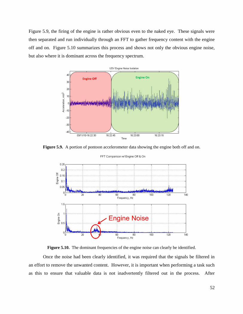
52

Figure 5.9, the firing of the engine is rather obvious even to the naked eye. These signals were

then separated and run individually through an FFT to gather frequency content with the engine

off and on. Figure 5.10 summarizes this process and shows not only the obvious engine noise,

but also where it is dominant across the frequency spectrum.

Figure 5.9. A portion of pontoon accelerometer data showing the engine both off and on.

Figure 5.10. The dominant frequencies of the engine noise can clearly be identified.

Once the noise had been clearly identified, it was required that the signals be filtered in

an effort to remove the unwanted content. However, it is important when performing a task such

as this to ensure that valuable data is not inadvertently filtered out in the process. After

53

analyzing the frequency content of the signal while the engine was on, it was decided that a

lowpass filter with a cutoff frequency at 30 Hz would be suitable for the test. A Butterworth-

style filter was chosen because it is maximally flat in the passband of the frequency response.

Also, as compared to Chebyshev or elliptical filters, the Butterworth filter does not possess

frequency response ripples in either the passband or stopband but has a slightly slower roll-off,

requiring the use of a higher order to mimic this characteristic. In this case a 5th

order

Butterworth filter was chosen to improve the roll-off rate into the stopband.

One issue still remained, however, because any digital filtering of the original time series

would result in a phase lag of the resultant signal. Considering that this input data would be used

to simulate response characteristics of the USV and then compared to time-series data from

testing, it was extremely important to eliminate this potential phase lag. The solution came in the

form of a zero-lag filtering scheme in MATLAB called filtfilt. This algorithm passes the data

through the designed filter twice (once in the intended direction and once in reverse) resulting in

zero-phase distortion and a filter order that is double the order of the originally designed filter.

This method was utilized for every filter applied to the data throughout analysis.

The ultimate goal of this stage of filtering is to produce clean model inputs, free of any

component of engine vibration, while ensuring that the signal’s phase content remains unaltered.

Figure 5.11 demonstrates this capability by showcasing the left front accelerometer raw and

filtered signals in the frequency domain as well as ten-seconds in the time domain. As the first

two subplots indicate, the filter does an excellent job of cutting out engine noise. The signal

remains visibly unchanged up to approximately 25 Hz before the roll-off becomes evident,

leaving the most important part of the signal intact. The final subplot indicates that the zero-

phase lag filtering scheme is working as designed. Each wave impact is clearly identifiable and

appears to be in phase harmony with the original signal.

54

Figure 5.11. The Butterworth lowpass filter clearly eliminates engine noise with little trouble.

5.4.2 Acceleration Integration

As previously mentioned, SimMechanics requires inputs of motion to be three-component

signals: acceleration, velocity and displacement. When working with discrete data such as this,

it is possible to integrate the acceleration signals with respect to time in either the time domain or

frequency domain. When performed in the time domain the integral is solved using a cumulative

trapezoidal numerical integration procedure, as taught in any college level calculus course. In

the frequency domain, however, the process is simplified into an arithmetic operation.

When a stochastic signal is integrated in the time domain, several forms of error can arise.

The most obvious source of integration error comes from the process of discretizing a continuous

signal in the first place. Figure 5.12 below displays an example of a continuous signal with a

trapezoidal integration overlaid in red. It is obvious from inspection that the results of this

integration will contain errors.

55

Figure 5.12. Discretization of continuous time-series signals leads to errors when a trapezoidal

integration scheme is applied.

Other forms of error, which may not be as obvious, stem from variations in the central tendencies

of original signal from zero. When integrated these variations are amplified as can be observed

in Figure 5.13. The plots on the left-hand side of this figure represent acceleration signals while

those on the right-hand side show their representative velocities after trapezoidal integration.

Equations (5-1), (5-2) and (5-3) were used to describe in the plot:

( ) (5-1)

( )

(5-2)

(

) ( ) (5-3)

The first signal has a constant mean of zero and is considered the baseline signal. The second

and third are variations to this signal with a DC offset and sine-on-sine respectively. It can be

observed that the original signal integrates correctly while the second creates a linear drift and

the third a sinusoidal drift. The more dangerous of these artifacts to this research is the sine-on-

sine phenomenon. The accelerometers utilized for this study operate in the frequency domain

down to DC (0 Hz), resulting in a DC-offset due to gravitational acceleration, which is removed

before integration. As the pontoons pitch and roll, this gravitational component will change

resulting in a similar type of sine-on-sine wave and an amplified error once integrated.

56

Figure 5.13. Integration error can stem from things such as a DC offset or other dynamic variations in

central tendency.

When the same integration process is performed in the frequency domain it solves down

to a simple arithmetic equation. Consider a time-series acceleration signal ( ) with frequency

content ( ) found by the Fourier transform. This relationship can easily be reversed with the

application of an inverse Fourier transform which converts the data from frequency back to time

domain. Therefore, the time series of the displacement data could be derived from the frequency

content of the displacement data. Conversion of the acceleration signal to displacement in the

frequency domain is performed by application of equation (5-4), which is derived in Appendix A.

( )

( )

(5-4)

57

The algorithm behind this equation states that at each individual frequency bin of the

Fourier series, the amplitude must be divided by the negative of that bin’s frequency squared.

This process avoids many of the errors innate to time series integration, but introduces one major

downfall at low frequency. The equation displayed above goes to infinity as the frequency

approaches zero. This phenomenon is commonly referred to as “ ⁄ noise”. In light of the

relatively low frequency content of the oceanic inputs and suspension response with respect to

the sampling rate, it was concluded that this integration method would not be applicable to the

USV testing data.

This decision meant that a reliable technique of compensation for time domain

integration error had to be formulated. After several failed attempts, a repeatable method was

developed which involved the application of a tuned highpass filter with a very low cutoff

frequency pre- and post-integration. Tuning of this cutoff frequency was performed empirically

using a very simple test. An accelerometer used during USV testing was mounted to the moving

clevis of a Rhoerig damper dynamometer. A string potentiometer was also mounted to the rig to

directly measure displacement of the clevis. These two signals were recorded with the same data

acquisition system and sampling rate utilized during USV testing to ensure comparable results.

A depiction of the testing setup is shown in Figure 5.14 below. In order to fully understand the

effects of varying cutoff frequency on this filter, a broad range of testing conditions were

planned. The inputs were to be of sinusoidal form, thus varying frequency and amplitude

became very important for this test. Table 5-3 outlines the testing procedures planned for

calibrating the cutoff frequency of the integration filter. After analyzing the effect cutoff

frequency has on integration results, it was decided to utilize a highpass Butterworth filter with a

cutoff frequency of Hz.

58

Figure 5.14. A damper dynamometer was outfitted with sensors to gather calibration data for the

integration filter. Photo by author, 2011.

Table 5-3

Integration Filter Calibration Test Procedure

7 2 1 0.5

0.1 3 min 3 min X X

0.2 2 min 2 min X X

0.5 2 min 2 min X X

1 2 min 2 min X X

2 2 min 2 min X X

5 X 1 min X X

10 X 1 min 30 sec X

20 X X X 30 sec

Amplitude (in)

Freq

uenc

y (H

z)

59

5.5 Single Degree of Freedom Modeling and Results

When designing a suspension, prediction of the system’s natural response frequency is

commonly desired or required before anything is built, in order to avoid exciting the system at its

resonant frequency. This can become a very difficult task in complex systems, making it

valuable to be able to derive this property from simple models. A single degree of freedom (1-

DOF) model of the USV was developed by taking the ship in the side view and assuming all

chassis motions are purely vertical. Figure 5.15 shows a diagram representing this 1-DOF model

where is the length from rear pivot to front suspension, is the length from rear pivot to CG,

is suspended mass and is double the suspension stiffness. Using this model, the natural

frequency was derived to be

√

√

(5-5)

where is defined as the length ratio, which for the case of the USV calculates to 2.14. The full

natural frequency derivation for this model can be found in Appendix B.

Figure 5.15. A 1-DOF model was developed to predict USV suspension response frequencies. Upper

photo by author, 2011.

60

As discussed in previous sections, the USV spring rate is very nonlinear with

displacement. In order to utilize the 1-DOF model, this spring force vs. displacement curve had

to be summarized with curve fitting techniques. Several options were considered including 1st,

2nd

and 3rd

order polynomials and an exponential fit, but the best results came from a

combination of 4 - 1st order polynomial (linear) fits as depicted in Figure 5.16. The red and blue

numbers within the boxes represent the spring stiffness and relative natural frequency as defined

by equation (5-5) above. The numbers located at the bottom of the figure represent statistical

displacement percentiles gathered from linear spring potentiometer data during testing. It can be

observed that the vast majority of suspension operation is spent at a natural frequency between

Hz and Hz (17th

and 95th

percentiles).

Figure 5.16. The spring force vs. displacement curve was simplified using 4 linear curve fits. The lower

numbers in the figure represent statistical displacement percentiles from testing.

Validation of this model required analysis of the frequency content of the spring linear

potentiometers. Due to the sensor failures mentioned previously, only a short amount of data

was available for this analysis; all of which occurs in head seas at full throttle. Once plotted, the

frequency response of the suspension potentiometers reveals interesting results. It is clear in

Figure 5.17 that this response contains two major regimes, one at approximately Hz and

another closer to Hz.

61

Figure 5.17. The frequency response of the linear spring potentiometer showcases both the input and

suspension response frequencies.

It is understood that systems excited at their base, such as the USV, will show oscillatory

response with components of both the input and response frequencies. In order to determine

which peak belongs to each component, the data was further analyzed in the time domain.

Figure 5.18 depicts two seconds of displacement data from the left front linear spring

potentiometer, where negative displacement indicates compression of the spring. In this figure

very large repetitive peaks at a fairly slow frequency are observed, each being followed by

smaller amplitude oscillations. These large peaks should represent individual wave impacts with

the ancillary suspension response resulting just afterward. With this assumption in mind, Figure

5.19 reveals that the wave impact frequency range revolves around approximately Hz while

the response frequency ranges from Hz to Hz. This outcome confirms the notion aroused

by the 1-DOF model results claiming a natural frequency range between and Hz.

62

Figure 5.18. Two seconds of linear spring potentiometer displacement data displaying both the impact

and suspension response frequencies.

Figure 5.19. As the data from Figure 5.18 is manually analyzed, it reveals the same frequencies found

from the Fourier analysis.

5.6 Multi-Body Dynamic Simulation Results and Validation

As discussed previously, the validation of simulation models is a critical step in the application

of those models into dynamic prediction algorithms. Validation of the USV multi-body dynamic

model was performed primarily in the time domain. Great emphasis was placed on ensuring

phase correlation between measurement and simulation, thus it was felt that analysis in the time

domain would best test the robustness of the model.

63

The first step in assessing the validity of the dynamic simulation was to investigate the

estimated linear damping rate as discussed previously in section 4.4. The USV model was

simulated at six different damping coefficients and responses were recorded for several

interesting parameters. Table 5-4 summarizes the damping coefficients and the corresponding

percentages from baseline used. For this analysis, the right front suspension displacement, right

front suspension velocity, and center of gravity vertical acceleration are displayed in the time

domain for each of the damping coefficients summarized below. Figures Figure 5.20, Figure

5.21, and Figure 5.22 show the responses, respectively. Each figure is organized in the same

order as shown in Table 5-4.

Table 5-4

Linear Damping Coefficients Tested for Assumption Validation

Damping Scenario

(% of Baseline)

Damping Coefficient

(

)

33 % 10

66 % 20

Baseline 30

200 % 60

300 % 90

400 % 120

64

Figure 5.20. Variation of right front spring displacement response due to damping coefficient.

45 46 47 48 49 50 51 52 53 54 55-5

0

5

33 %

Observation

Simulation

45 46 47 48 49 50 51 52 53 54 55-5

0

5

66 %

45 46 47 48 49 50 51 52 53 54 55-5

0

5

Base

45 46 47 48 49 50 51 52 53 54 55-5

0

5

200 %

45 46 47 48 49 50 51 52 53 54 55-5

0

5

300 %

Effects of Linear Damping Variation on RF Spring Displacement (in)

45 46 47 48 49 50 51 52 53 54 55-5

0

5

400 %

Time, s

65

Figure 5.21. Variation of right front spring velocity response due to damping coefficient.

45 46 47 48 49 50 51 52 53 54 55-100

0

100

33 %

Observation

Simulation

45 46 47 48 49 50 51 52 53 54 55-100

0

100

66 %

45 46 47 48 49 50 51 52 53 54 55-100

0

100

Base

45 46 47 48 49 50 51 52 53 54 55-100

0

100

200 %

45 46 47 48 49 50 51 52 53 54 55-100

0

100

300 %

Effects of Linear Damping Variation on RF Spring Velocity (in/s)

45 46 47 48 49 50 51 52 53 54 55-100

0

100

400 %

Time, s

66

Figure 5.22. Variation in center of gravity vertical acceleration response due to damping coefficient.

45 46 47 48 49 50 51 52 53 54 5530

0

30

33 %

Observation

Simulation

45 46 47 48 49 50 51 52 53 54 55-30

0

30

66 %

45 46 47 48 49 50 51 52 53 54 55-30

0

30

Base

45 46 47 48 49 50 51 52 53 54 55-30

0

30

200 %

45 46 47 48 49 50 51 52 53 54 55-30

0

30

300 %

Effects of Linear Damping Variation on CG Vertical Acceleration (m/s2)

45 46 47 48 49 50 51 52 53 54 55-30

0

30

400 %

Time, s

67

As would be expected, the lightly damped simulations exhibit increased overshoot and

oscillatory motions not present in the measured data while the heavily damped responses are

slow to respond and show some undercutting of observed peaks. This is more prevalent in the

right front suspension displacement and velocity responses of Figures Figure 5.20 and Figure

5.21 than the vertical acceleration response of Figure 5.22. The most obvious changes can be

seen in the velocity response, which makes sense because this motion directly drives the

damping forces of the vessel. The displacement response shows a much greater effect when the

damping is reduced from baseline rather than increased. When browsing the response traces

from vertical acceleration, however, these same trends become much more difficult to find. At

extrema, such as the 3g peak just before 50 seconds, the effects can be identified, but most other

areas in the time series are very insensitive to changes in damping. Cabin vertical acceleration

response is probably the most important value to be able to predict for this study and this model

seems to be very robust in that manner. It should be noted that despite any sensitivities of the

model to damping variation, the estimated baseline damping coefficient developed in section 4.4

produces extremely accurate results for all three motions.

The next step of the validation process was to directly compare the simulated and actual

response of several output sensors. Figure 5.23 represents the cabin acceleration, central joint

rotational displacement and both suspension displacements for 10 seconds. Measured data is

represented in blue with simulated data in red. From a general perspective, all of the simulated

responses appear to readily emulate the measured responses from the test vessel.

68

Figure 5.23. In the time domain the USV simulation appears to very accurately represent the realistic

testing measurements.

The most accurate fitment of reality to simulation comes from the cabin accelerometer.

This is very promising because this reading is one of the most important to be able to properly

simulate. Both the left and right suspension potentiometer figures at the bottom show extremely

well matched results while the rotational measurement of the top right shows slightly greater

error, but very promising response trends.

69

Chapter 6

Concluding Remarks

During the course of this research, two dynamic simulation models were created in

SimMechanics. The kinematically constrained Proteus model successfully produced common

trends associated with particular parameter variations. The simpler USV dynamic model was

validated in the time domain with test data. This data was used to create representative inputs to

the model and as a comparison to simulated outputs. The following chapter will highlight the

successes and shortcomings of these models, simulations, and studies and provide

recommendations for future research in this field.

6.1 Summary and Discussion

6.1.1 Parametric Analysis of Proteus

The Proteus dynamic simulation model worked well as a tool to predict trends resulting from

variations in important dynamic parameters, but also had several drawbacks. Due to the method

in which the Proteus dynamic model was imported from CAD, the kinematics could not be

varied. This limited the parametric analysis from delving into the effects of variations on basic

ship architecture and only allowed for the study of spring rates, damping coefficients and mass

properties. This restriction, however, comes with the benefits that the kinematic constraints and

baseline mass and mass location are very accurate. It should also be noted that these results did

not come from stochastic ocean inputs, but rather from simple periodic waves. Pure heave and

pitch modes are idealized cases where the vessel speed, wave speed and wavelength are matched

perfectly under head sea conditions. Any real oceanic input, even in the head sea direction, will

most likely result in some combination of all four excitation modes.

70

The heave excitation will produce the best results for analyzing the effect that the

suspension has directly upon the cabin motion. When the vessel is driven in other modes, more

kinematic relationships come into play with the cabin response. This is obvious due to the fact

that the vertical CG position plays a drastically more significant role on the vertical acceleration

from pitch than heave. Also, the increased absolute sensitivity of the rear spring rate from pitch

excitation as sensed by the rear accelerometer indicates that this effect may be taking place. In

general, the sensitivity results match up to common sense results very well. As can be seen in

the summary of parametric analysis findings presented in Table 6-1, the springs play the greatest

role on accelerations felt closest to that suspension, while the mass properties affect the areas

closest to the sprung mass CG. It should be noted that the variation of damping provided

negligible effects on response, which could be a result of the minute baseline damping

coefficient.

Table 6-1

Summary of Parametric Analysis Results

Parameter Primary

Relation Most Sensitive Position

Spring Rate Inverse At end closest to the

relative suspension

Mass Direct Closest to sprung mass CG

CG Long Inverse Closest to sprung mass CG

CG Vert * Direct Closest to sprung mass CG

* Indicates that this parameter is only sensitive under pitching excitation

These trends should be indicative of parametric variations of any vessel very similar to

Proteus, but the results also must be taken with a grain of salt. The springs on Proteus are

71

extremely non-linear and all damping is a result of friction in the joints and sliding members. In

the parametric model, these effects are assumed to be completely linear. Because of this, the

simulated percentage sensitivities are probably not indicative of the results as they would be seen

on Proteus because of the effects of non-linearity, however the trends and primary relationships

should hold true.

6.1.2 USV Modeling & Validation

The validation results from the stochastically excited USV dynamic model show excellent

agreement to testing data. Although this model appears to be very simple in comparison to the

detailed Proteus model it retains a high level of accuracy for the most important properties

including mass, CG location, spring rates, and polar inertia in primary directions of rotation. The

USV dynamic simulations run very quickly and are an excellent substitute for costly and time-

consuming testing. The single-DOF model also showed a great deal of agreement with testing

data in the frequency domain. This proved the validity of the spring rates being applied to the

dynamic model and gave insight into the primary range of motion and natural response

frequencies of the vessel.

The major limitation of the dynamic USV model, however, comes from the method in

which the inputs were applied. By choosing to neglect hydrodynamic effects the inputs to the

model were required to come from data collected directly on the pontoons of a test vessel. This

condition is a result of the codependent relationship between any hull and the water it is passing

through. As the hull is being affected and moved by a passing wave, it is also physically

degrading the local wave structure. This essentially means that the model inputs are limited in

scope to only properly excite the specific USV arrangement. Any change in basic configuration

or major parameter alteration would lead to a different water/hull response dynamic and would

produce different inputs at the pontoons.

The time-series results of the USV model validation are extremely promising. Although

the input data is being filtered and integrated several times, the outputs match the test data

remarkably well in amplitude, shape, and phase. The most promising results come from the

vertical acceleration at the cabin. This is the most important signal to match for analyzing

72

passenger comfort and shows the tremendous prediction power of the USV SimMechanics model.

Both suspension potentiometers also reveal excellent response matching. The slight error

between the measured and simulated linear potentiometer signals could be the result of the

assumptions made when deriving the spring force characteristics from the raw data or minor

errors coming to the surface from the integration and filtering of the inputs. The worst matched

dataset is the relative rotational displacement of the front arch with respect to the payload tray.

Even this signal, however, produces very well matched results with the increase in error

potentially coming from several factors including those mentioned above for the linear

potentiometer error as well as the probable fact that some components’ polar inertias in the

simulation did not match their respective parts on the real vessel as well as was initially hoped.

6.2 Recommendations

Further simulation development of WAM-Vs™ will be required before its full benefit can be

realized. As stated previously, the primary limiting factor of the dynamic model in its current

state is the lack of a hydrodynamics solver. The model showed excellent capabilities to predict

chassis motions so long as reliable inputs could be applied. Without the ability to solve for the

water/hull interaction the scope of these simulations will limit them from their true potential of

replacing expensive on-water testing.

Although the USV model provided acceptable enough results to prove its potential

validity, the breadth of comparable testing data was extremely limited. Future testing should

include variations in suspension stiffness and damping, payload mass and location, and even

basic ship configuration. This enlarged scope should provide the necessary data to ensure the

validity of dynamic simulations to predict WAM-V™ motions. In addition, the multitude of

parameter variations would provide an excellent basis for tuning model parameters, thereby

increasing prediction accuracy.

Future WAM-V™ testing platforms should be made adaptable for “locking out”

particular components such as the suspensions or main ball joint. The relationship between

73

simple catamarans and WAM-Vs™ is not well known at this time; therefore the impact of each

architectural variant on the change in vessel response needs research. Having the ability to

essentially eliminate particular systems and to even force the configuration to be a simple

catamaran supplies the user with insight into the effect of each component onto the total vessel

response. This information could be used as a guide for resource allotment in the design of

future WAM-Vs™.

The final recommendation for future testing of WAM-Vs™ is to make an effort to study

the difference in response of the vessel to ocean swell (ground swell) and wind swell. Ocean

swell originates from far-off storms or wind-systems and results in waves that are very stable in

their direction and frequency whereas wind swell comes from local winds and produces more

chaotic waves with faster and more variant frequency. These two excitation sources could

produce very different results, but both need to be understood. This could easily be achieved

with testing in open-ocean followed by a bay or other body which is protected from ocean swell,

but large enough to show significant wind swell.

74

Appendices

Appendix A

Acceleration Integration – Omega Arithmetic

Let us define ( ) and ( )as the time- and frequency-domain acceleration signals, respectively.

The frequency spectra of any time-based signal can be found with the Fourier transform, which

can also be inverted to revert back from the frequency to time domain. Using the inverse Fourier

transform, the following relations can be made for acceleration, velocity and displacement.

( ) ∫ ( )

( ) ∫ ( )

( ) ∫ ( )

Using these relationships, the association made between velocity and acceleration in the time

domain can be extended into the frequency domain.

( )

[ ( )]

( )

[∫ ( )

]

∫ ( )

[ ]

∫ ( )

75

When this results is compared back to the Fourier transform representation of ( ) it can be seen

that

( ) ( )

( ) ( )

( )

When this concept it applied to the conversion from displacement to acceleration, the following

results is found.

( ) ( ) ( ) ( )

76

Appendix B

USV Single-DOF Model

To analyze the natural response frequency of the USV chassis a basic single-DOF model was

created. The USV was modeled as a beam pinned at one end and sprung at the other. The

diagram of Figure B-1 displays this simplified representation for the USV chassis dynamics. By

creating a balance of moments about the pivot point an equation of motion can be created to find

the natural response frequency.

Figure B-1. The USV was modeled as a pinned-and-cantilevered beam with a spring opposite the pin.

Upper photo by author, 2011.

77

By utilizing the small-angle assumption the following equations spell out the derivation for

solving the USV natural frequency.

( )

( ) ( )

( ) ( )

√ ( )

( ) √

For the USV case, and , therefore

√

78

References

[1] Baitis, A. E. et al. 1975. “A Seakeeping Comparison Between Three Monohulls, Two

Swaths, and a Column-Stabilized Catamaran Designed for the Same Mission.” NTIS

(July).

[2] Bautista, J., Kuehne, H., Irvine Jr., M., & Riley, M. 2009. “Marine Advanced Research

WAM-V PROTEUS Propulsion, Seakeeping, and Miscellaneous Trials.” Naval Surface

Warfare Center Carderock Technical Memorandum. NSWCCD-23-TM-2009/43.

[3] Bonafoux, J., Edward Dudson, and D. Sherwood. 2001. “An Evaluation of the Effect of

Hull Form Choice on the Operability of Fast Ferries.” Fast 2001 Conference.

Southampton, England, September.

[4] Bulian, Gabriele, and Alberto Francescutto. 2008. “Large amplitude rolling and strongly

nonlinear behaviour of multihull ships in moderate beam waves.” IUTAM Symposium on

Fluid-Structure Interaction in Ocean Engineering.

[5] Clark, Dennis J, William M Ellsworth, and John R Meyer. 2004. “The Quest for Speed at

Sea.” NSWC Carderock Division - Technical Digest: 3-27.

[6] Davis, M R, and D S Holloway. 2003. “The influence of hull form on the motions of high

speed vessels in head seas.” Ocean Engineering 30: 2091-2115.

[7] Dubrovsky, Victor, and Konstantin Matveev. 2005. “New Types of Sea-Going Multi-

Hull Ships with Superior Comfort Level and Safety.” Passenger Vessels for the New

Millenium: Joint Meeting of the Pacific Region Sections: 1-12.

[8] Dyachkov, Vasilij, and Jurij Makov. 2005. “Seakeeping of a fast displacement catamaran.”

Transport XX(1): 14-22.

[9] Fang, C.C., and H.S. Chan. 2004. “Investigation of Seakeeping Characteristics of High-

Speed Catamarans in Waves.” Journal of Marine Science and Technology 12(1): 7–15.

[10] Kos, Serđo, D. Brčić, and Vlado Frančić. 2009. “Comparative Analysis of Conventional

and SWATH Passenger Catamaran.” Proceedings of International Conference on

Transport Science. Portorož, Slovenia. p. 4–5.

[11] Nagai, Tamotsu. 1987. “Critical Review of SWATHs.” Research Reports of Ikutoku Tech.

Univ B-11: 1-21.

[12] Thomas, G., P. Tomic, and a. Tuite. 2007. “High-speed catamaran or monohull? How do

you choose?” Ships and Offshore Structures 2(2): 137-147.

79

[13] Turan, Osman, Chirstos Verveniotis, and Hassan Khalid. 2009. “Motion sickness

onboard ships: subjective vertical theory and its application to full-scale trials.” Journal

of Marine Science and Technology 14(4): 409-416.

[14] Varyani, K. 2000. “Motions and slamming impact on catamaran.” Ocean Engineering

27(7): 729-747.