econstorMake Your Publications Visible.

A Service of

zbwLeibniz-InformationszentrumWirtschaftLeibniz Information Centrefor Economics

Chen, Yu-wang et al.

Working Paper

Multi-asset portfolio optimisation using a belief rule-based system

Manchester Business School Working Paper, No. 603

Provided in Cooperation with:Manchester Business School, The University of Manchester

Suggested Citation: Chen, Yu-wang et al. (2010) : Multi-asset portfolio optimisation using abelief rule-based system, Manchester Business School Working Paper, No. 603, The Universityof Manchester, Manchester Business School, Manchester

This Version is available at:http://hdl.handle.net/10419/50667

Standard-Nutzungsbedingungen:

Die Dokumente auf EconStor dürfen zu eigenen wissenschaftlichenZwecken und zum Privatgebrauch gespeichert und kopiert werden.

Sie dürfen die Dokumente nicht für öffentliche oder kommerzielleZwecke vervielfältigen, öffentlich ausstellen, öffentlich zugänglichmachen, vertreiben oder anderweitig nutzen.

Sofern die Verfasser die Dokumente unter Open-Content-Lizenzen(insbesondere CC-Lizenzen) zur Verfügung gestellt haben sollten,gelten abweichend von diesen Nutzungsbedingungen die in der dortgenannten Lizenz gewährten Nutzungsrechte.

Terms of use:

Documents in EconStor may be saved and copied for yourpersonal and scholarly purposes.

You are not to copy documents for public or commercialpurposes, to exhibit the documents publicly, to make thempublicly available on the internet, or to distribute or otherwiseuse the documents in public.

If the documents have been made available under an OpenContent Licence (especially Creative Commons Licences), youmay exercise further usage rights as specified in the indicatedlicence.

www.econstor.eu

Working Paper Series

Multi-asset class portfolio optimisation using a belief rule-based system Yu-Wang Chen, Jian-Bo Yang, Dong-Ling Xu, Dongxu Zhang, Simon Acomb and Ser-Huang Poon Manchester Business School Working Paper No. 603 July 2010

Manchester Business School Copyright © 2010, Chen, Yang, Xu, Zhang, Acomb and Poon. All rights reserved. Do not quote or cite without permission from the author. Manchester Business School The University of Manchester Booth Street West Manchester M15 6PB +44(0)161 306 1320 http://www.mbs.ac.uk/research/working-papers/default.aspx ISSN 0954-7401 The working papers are produced by The University o f Manchester - Manchester Business School and are to be circulated for discussion purposes only. Thei r contents should be considered to be preliminary. The papers are expected to be published in due course, in a revised form and should not be quoted without the authors’ permission.

Author(s) and affiliation Yu-Wang Chen, Jian-Bo Yang, Dong-Ling Xu, Dongxu Zhang, Simon Acomb and Ser-Huang Poon Manchester Business School The University of Manchester Manchester, M15 6PB UK Keywords Belief rule base, evidential reasoning, asset class, portfolio optimisation Abstract The purpose of this paper is to apply a belief rule-based (BRB) system to solve the multi-asset class portfolio optimisation problems. The BRB system, was developed on the basis of the concept of belief structures and the evidential reasoning (ER) approach, is a generic non-linear modelling and inference scheme. In this paper, the procedures of implementing the BRB system with RiskMetrics WealthBench to portfolio optimisation are discussed in details. Two different ways are proposed to locate the optimal portfolios under constraints supplied by the investors. Numerical studies demonstrate the effectiveness and efficiency of the proposed methodology. How to quote or cite this document Chen, Yu-Wang, Yang, Jian-Bo, Xu, Dong-Ling, Zhang, Dongxu, Acomb, Simon and Poon, Ser-Huang. (2010). Multi-asset class portfolio optimisation using a belief rule-based system. Manchester Business School Working Paper, Number 603, available: http://www.mbs.ac.uk/research/working-papers.aspx.

Multi-asset class portfolio optimisation using a belief rule-based system

Yu-Wang Chen, Jian-Bo Yang, Dong-Ling Xu, Dongxu Zhang, Simon Acomb, Ser-Huang Poon

Manchester Business School, The University of Manchester, Manchester M15 6PB, UK

Abstract. The purpose of this paper is to apply a belief rule-based (BRB) system to solve the multi-asset class portfolio optimisation problems. The BRB system, was developed on the basis of the concept of belief structures and the evidential reasoning (ER) approach, is a generic non-linear modelling and inference scheme. In this paper, the procedures of implementing the BRB system with RiskMetrics WealthBench to portfolio optimisation are discussed in details. Two different ways are proposed to locate the optimal portfolios under constraints supplied by the investors. Numerical studies demonstrate the effectiveness and efficiency of the proposed methodology. Keywords: Belief rule base, evidential reasoning, asset class, portfolio optimisation.

1. Introduction Portfolio optimisation is concerned with implementing investment strategy and information technology to maximise the wealth of investors and manage the risk of an integrated portfolio over a fixed-term period. In the process of implementing an investment strategy, multi-asset class allocation is the most crucial decision required to achieve the investment goals of high returns and low risks (Kritzman, 1999; Gratcheva and Falk, 2003). In the past decades, many studies have shown that strategic asset allocation has more influence on the aggregate portfolio return than other investment decisions and usually explains most of its return variations over a long-term period (Brinson et al., 1986; Hensel et al., 1991; Ibbotson and Kaplan, 2000). Asset allocation usually produces a set of portfolio weights for multiple asset classes such as stocks and bonds, and this diversification strategy is beneficial to both return enhancement and volatility reduction. As the basis of modern portfolio theory, the seminal Markowitz’s mean-variance model provides a useful theoretical framework to solve strategic asset allocation problem (Markowitz, 1952). It suggested that an investor should make a trade-off between return and risk in determining the allocation of assets. Among an infinite number of investment portfolios with a specific return objective, the investor should choose the portfolio that has the smallest variance or risk, and all other portfolios are “inefficient” because they have higher variance at a given level of return. Although Markowitz's optimisation model provides a parametric methodology for asset allocation and portfolio diversification, it has not been widely used in practice due to a number of practical and theoretical problems associated with it. In mean-variance analysis, the assumption of normal distribution of returns may not be accurate under some scenarios, and it is difficult to measure the necessary inputs, namely expected returns, variances and co-variances of risky assets (Bawa, 1975; Jorion, 1991; Kan and Zhou, 2007). In addition, the original Markowitz model ignores environmental factors (e.g., tax and transaction cost) and assumes a single-period

investment horizon. However, in reality, investments are usually multi-period, and optimal portfolio decisions, especially for long-term investors, depend on the details of the changing investment environment, such as the available financial assets, the taxation, and the expected returns and preferences of investors (Campbell and Viceira, 2002). Furthermore, multi-period portfolio optimisation problem needs scenario simulation analysis to forecast expected returns (Markowitz and Perold, 1981; Koskosidis and Duarte, 1997). As such, a series of theoretical work has been conducted to improve portfolio optimisation models on the basis of mean-variance analysis (Black and Litterman, 1992; Tütüncü and Koenig, 2004; Ehrgott et al., 2004; Jacobs et al., 2005; Kim et al., 2005; Idzorek, 2006; Çelikyurta and Özekici, 2007). Simultaneously, various simulation techniques using historical data or Monte Carlo algorithm have been used to forecast the portfolios with nonlinear instruments such as options (RiskMetrics, 1999; 2004; Palmquist et al., 2001; Glasserman, 2004; Brandt et al., 2005). In allocating investment to a number of asset classes, the optimisation objective depends on investors’ financial needs and actual investment scales. The relationship between the proportion of each asset class in a portfolio and the distribution of its return is highly nonlinear (Campbell and Viceira, 2002; RiskMetrics, 2004). To identify the optimal combination of asset classes in order to maximise returns and minimise risks, there is a need to develop a method which can model such a highly nonlinear relationship. This paper is dedicated to developing a novel portfolio modelling and optimisation method using a belief rule-based (BRB) system. The BRB system was developed on the basis of the concept of belief structures and the evidential reasoning (ER) approach (Yang and Singh, 1994; Yang et al., 2006; 2007). It has been widely applied in fields of nonlinear system identification and decision support systems (Xu et al, 2007; Zhou et al., 2009; Chen et al., 2010). The rest of the paper is organised as follows: in the following section, the portfolio optimisation problem is modelled using a BRB system, and the detailed procedures are discussed. In Section 3, on the basis of the BRB system, two portfolio optimisation methods are presented to locate the optimal portfolio under different constraints. In Section 4, Numerical studies are conducted to demonstrate the effectiveness and efficiency of the developed BRB system to portfolio optimisation. The paper is concluded in Section 5.

2. Modelling portfolio optimisation with a BRB system Portfolio optimisation is to build the allocation of asset classes which maximizes the return for a given level of risk or minimizes the risk for a given level of return (Bekkers et al., 2009). Generally, an asset class is a set of assets with some fundamental economic similarities (Greer, 1997). Portfolios are usually represented in terms of asset classes rather than assets because it is widely believed that the asset class returns can be forecasted more accurately than asset returns and asset returns tend to revert to asset class returns in the long-term simulation (RiskMetrics, 2004). Suppose there are M asset classes, we can model an asset class portfolio by a vector of non-negative weights ),...,,( 21 Mwww , where iw represents the proportion of the total

wealth to be invested in the ith asset class. In other word, if iv represents the current

market value of the total investment in the ith asset class, then )...( 1 Mii vvvw ++= .

Thus, the portfolio optimisation problem is transformed to determining the optimal weights of asset classes. To apply a BRB system to model and solve the portfolio optimisation problem, we need to explain some basic theoretical concepts at first. Belief rules are the central constituents of BRB systems, and they usually are designed with an extended IF-THEN scheme, in which each possible consequent is associated with a belief degree. In portfolio optimisation, formally, the kth belief rule ),...,1( KkRk = can be defined as follows,

{ }

{ }.,...,1,,...,, weight attribute and

, weight rulewith

,1,),(),...,,(),,( THEN

), is ( ) is ( ) is ( IF

:

,,2,1

1,,2,21,1

2211

Kk

DDD

AwAwAw

R

kMkk

k

N

nnkNkNkk

kMM

kk

k

∈

≤

∧∧∧

∑=

δδδθ

ββββ

L

(1)

where Mwww ,...,, 21 denote the antecedent attributes in the kth rule. Each attribute

takes values from { }MAAA ,...,1= , in which each of the element ),...,1( MiAi = is

defined by a set of referential values { }ijii NAjAA ,...,1;, == . In the kth rule, kiA

represents the referential value taken by the attribute iw , and { }ijiki NAjAA ,...,1;, =∈ .

nk,β is the belief degree associated with consequent nD given the logical relationship

of ) is ( ) is ( ) is ( 2211kMM

kk AwAwAw ∧∧∧ L . kθ is the relative weight of the kth rule,

and kMkk ,,2,1 ,...,, δδδ are the relative weights of the M antecedent attributes in the kth

rule. In portfolio optimisation problem, the antecedent attributes iw are the weights of

asset classes, and the consequents are portfolio returns grouped by buckets (i.e., ranges of values). As such, we can use a BRB system to model and solve the optimisation problem with the following main steps: (1) constructing belief rules; (2) calculating activation weights; (3) generating new portfolios through BRB interpolation. Here, it is worth noting the BRB interpolated outputs are characterised by the belief distribution ),...,,( 21 Nβββ .

2.1 Constructing belief rules with linear bounds and unity constraint

In the portfolio optimisation problem, the decision variables are the weights of asset classes, which are usually subject to two types of constraints. First of all, the sum of all asset weights should be equal to 1 or 100%. Secondly, individual or institutional investors may also specify upper or lower boundaries of weights to some major asset classes for business reasons. For example, an investor may recommend portfolios with at least 20% wealth in large capital stocks, or wish that all portfolios have between 30% and 50% wealth invested in equities. Thus, we need to consider these bounds and unity constraints when constructing the initial belief rule base to model the portfolio optimisation problem.

2.1.1 Generating referential rule points

Let ilb and iub represent the lower and upper bound of the weight for the ith asset

class respectively, and then the linear bounds and unity constraint can be represented as follows, iii ubwlb ≤≤ (2)

11

=∑=

M

iiw (3)

Generally speaking, when constructing an initial belief rule base, it is necessary to sample some referential rule points in the feasible solution space. If the space is two or more dimensional, usually, we select a few referential values on each dimension, or equivalently, for each independent variable, and the referential rule points are generated by the combination of the referential values of all the independent variables. Those variables are input decision variables to the BRB system. In portfolio optimisation, using the unity constraint of equation (3), we can reduce the number of dimensions of the solution space by one, and the weight Mw of the Mth asset class can be represented as,

∑−

=−= 1

11

M

i iM ww (4)

That means the number of independent decision variables becomes 1−M . Furthermore, we check the conflicts among the bound constraints and adjust the initial lower and upper bounds for all asset classes. To illustrate the necessity of adjusting initial bounds, two examples are given below. Example 1. Suppose there are 2 asset classes, and the bound constraints are given as follows. 10 1 ≤≤ w

12.0 2 ≤≤ w

We uniformly select three referential values from the feasible interval of 1w , and

those are 0, 0.5 and 1. As shown in Fig.1(a), the referential value 11 =w corresponds

to the weight combination )0,1(),( 21 =ww , which is an infeasible referential point.

0 0.5 1

0.2

1A

2A

0.2

1A

2A

0 0.4 0.8

1 1

(a) (b) Fig. 1 Two asset class example with upper bound adjustment

To make sure that the referential points are in the feasible space, the upper bound of

1w should be adjusted to 0.8 as shown in Fig. 1(b). Three feasible referential values 0,

0.4 and 0.8 can be selected for 1w after the bound adjustment. Example 2. Suppose there are 2 asset classes, and the bound constraints are given as follows. 10 1 ≤≤ w

2.00 2 ≤≤ w

If we also uniformly select three referential values from the feasible interval of 1w , two referential values 0 and 0.5 will be infeasible as shown in Fig. 2 (a).

0 0.5 1

0.2

1A

2A

0.2

1A

2A

0.8 0.9 1

(a) (b) Fig. 2 Two asset class example with lower bound adjustment

Similarly, the lower bound of 1w should be adjusted to 0.8, and three feasible referential values of 0.8, 0.9 and 1 can be sampled as Fig. 2 (b). For a multiple input system, or a portfolio with more than two asset classes, it is difficult to adjust the lower and upper bounds manually. The following equations,

however, can be used systematically to produce the bounds ilb and iub for each asset class so that the conflicts among bound constraints can be eliminated.

)1,max(,1∑

≠=

−=M

ijjjii ublblb (5)

)1,min(,1∑

≠=−=

M

ijjjii lbubub (6)

Furthermore, if there are more than 2 asset classes, we need to consider the unity

constraint, i.e., 11

=∑ =

M

i iw , when selecting referential values for the weight of each

asset class in order to generate feasible referential points. An illustrative example is given as follows. Example 3. Suppose there are 3 asset classes, the bound constraints are without conflicts and given as follows. 6.00 1 ≤≤ w

8.02.0 2 ≤≤ w

8.01.0 3 ≤≤ w

As discussed above, the weight 3w can be decided by the sum of 1w and 2w using

equation (4). Therefore, we can use the combination of the referential values of 1w

and 2w to construct the initial belief rule base. Assume the referential values of 1w are {0, 0.3, 0.6} and that of 2w are {0.2, 0.5, 0.8}. Without the unity constraint, 3×3 referential points will be generated as shown in Fig. 3(a).

1A

2A

1A

2A

Fig. 3 Three asset class example with projecting new rule points

However, some of the points, (0.3, 0.8), (0.6, 0.5) and (0.6, 0.8) in Fig. 3(a), are not within the feasible solution space which is constrained by the following inequality constraints,

MM

i i lbw −≤∑−

=1

1

1 (7)

MM

i i ubw −≥∑−

=1

1

1 (8)

If we delete the infeasible points directly, the BRB inference accuracy near those deleted referential points will decrease since fewer referential belief rules are available. As such, some new referential points should be generated to replace them as shown in Fig. 3(b). To replace the infeasible referential point (0.3, 0.8), two new referential points (0.1, 0.8) and (0.3, 0.6) are generated by projecting it to the boundary of the feasible space. Similarly, two new referential points (0.4, 0.5) and (0.6, 0.3) are generated to replace the infeasible referential point (0.6, 0.5). No new referential points need to be generated for the infeasible referential point (0.6, 0.8), since it projects overlapped referential points (0.1, 0.8) and (0.6, 0.3). To a multi-asset class portfolio optimisation problem, a generic method needs to be proposed to generate new projected referential points for replacing infeasible points effectively. Here, it is worth noting that we need to consider the downward projection

onto the feasible boundary MM

i i lbw −=∑−

=1

1

1 and the upward projection onto

MM

i i ubw −=∑−

=1

1

1 simultaneously in generating projected referential points.

We first consider the downward projection onto MM

i i lbw −=∑−

=1

1

1. Suppose

imiA , is

the referential value taken by iw in an infeasible referential point with

∑−

=−>1

1 , 1M

iMmi lbA

i, where { }ijimi NAjAA

i,...,1;,, =∈ , and )1( ≥ii mm is an integer

and denotes the order number in the vector of referential values. In Example 3, the vector of referential values for 1w is (0, 0.3, 0.6). For the referential point (0.3, 0.8),

1m is equal to 2 since the second referential value 0.3 is taken by 1w . With this definition of im , we can generate new projected referential points to replace

any infeasible referential point with ∑−

=−>1

1 , 1M

iMmi lbA

i by reducing the weights of

the 1−M asset classes one by one. For iw , if 1>im and

MM

ijj mjmi lbAAji

−<+∑−

≠=− 11

,1 ,1, , a new referential point will be generated in which the

referential value of iw is projected to be ∑−

≠=−− 1

,1 ,1M

ijj mjMj

Alb ; otherwise, no new

referential point will be projected. In the above example, the referential point (0.3, 0.8) is infeasible, since the sum of

referential values is ∑−

==+=1

1 , 1.18.03.0M

i mi iA , which is larger than

9.01.011 =−=− Mlb . Therefore, we use the above-mentioned method to generate new projected referential points to replace it. For 1w , we have 21 =m and

8.08.001

,1 ,1, =+=+∑−

≠=−M

ijj mjmi jiAA , which is less than 0.9. Its projected weight for 1w

can be calculated by 1.08.01.0111

,1 , =−−=−− ∑−

≠=

M

ijj mjMj

Alb , and a new referential

point (0.1, 0.8) can be generated from it. For 2w , we have 32 =m and

8.03.05.01

,1 ,1, =+=+∑−

≠=−M

ijj mjmi jiAA , which is less than 0.9. Its projected weight can

be calculated by 5.03.01.0111

,1 , =−−=−− ∑−

≠=

M

ijj mjMj

Alb , and another new

referential point (0.3, 0.6) can be obtained. As a result, two new referential points (0.1, 0.8) and (0.3, 0.6) are used to replace the infeasible referential point (0.3, 0.8). Similarly, we can generate new projected referential points to replace any infeasible

referential point with ∑−

=−<1

1 , 1M

iMmi ubA

i. For iw , if ii NAm ≤ and

MM

ijj mjmi ubAAji

−>+∑−

≠=+ 11

,1 ,1, , a new referential point will be generated in which the

referential value of iw is projected to be ∑−

≠=−− 1

,1 ,1M

ijj mjMj

Aub ; otherwise, no new

referential point will be projected. With this method, it is obvious that the maximum number of new projected referential points for replacing each infeasible rule point is no more than 1−M (i.e., the number of asset classes minus 1), and the minimum number is 0. For example, in Fig. 3(b), the number of projected referential points for the infeasible referential points (0.3, 0.8) and (0.6, 0.5) is 213 =− , and that for the infeasible referential point (0.6, 0.8) is 0.

2.1.2 Constructing belief degrees for referential portfolios

In applying BRB systems to portfolio optimisation, we use belief distribution to approximate the distribution of the consequential portfolio returns. Belief degrees on

consequents can be obtained with historical and simulated data. In this paper, we use RiskMetrics WealthBench (RM-WB) platform (RiskMetrics, 2004) to simulate a set of 500=L observed returns LlRk

lP ,...,1,, = for the kth set of portfolio weights that

has the following mean and variance:

∑=

=L

l

klP

kP R

LRE

1,

1)( (9)

∑∑==

−=L

l

klP

L

l

klP

kP R

LR

LR

1

2,

1

2, )

1()(

1)var( (10)

It is worth noting that this pair of mean and variance is not used in portfolio optimisation apart from serving as a check for the bucket distribution below. As shown in Fig. 4, we group the simulated portfolio returns into 1−N buckets of consequents using N referential values NDDD ,...,, 21 within the range of portfolio

returns. Note that the buckets could be non-uniformly distributed.

Fig. 4 Belief distribution on buckets of consequents

For the kth belief rule, we can simply put k lPR , into the buckets and obtain the

probability of observed returns falling into each bucket, which is further used to be the belief degree on the corresponding buckets of consequents. However, since the actual value of observed returns in each bucket has not been considered in this way, the expected return can not be calculated accurately with the belief distribution. As a consequence, in this study we use the following equation to calculate the belief degree,

=−−

<<

−−+−−

=−−

=

∑

∑∑

∑

−−

−

−−

−

∈−−

∈++

∈−−

∈++

NnDDDRL

NnDDRDDDDRL

nDDRDL

nn

n

nn

n

nn

n

nn

n

Llnnn

klP

Llnn

klPn

Llnnn

klP

Llnn

klPn

nk

11

1

11

1

),/()(1

1,)/()()/()(1

1),/()(1

11,

1,111,

1,1

,β (11)

where nnnk

lPn LlDRDn

∈∀<≤ + ,1, . Obviously, we have 11 , =∑ =

N

n nkβ , and it is possible

that some 0, =jkβ . Using the belief degrees, the mean and variance of expected

returns represented by the belief distribution in the kth belief rule can be calculated as follows,

∑=

=N

nnknk DPE

1,)( β (12)

2

1,

1,

2)()var(

−= ∑∑==

N

nnkn

N

nnknk DDP ββ (13)

Combined with the equation (11), we can conclude that the returns calculated in equations (9) and (12) will be equal, but the variances in equations (10) and (13) will not necessarily be equal. The deviation between the statistical variance and approximated variance depends heavily on the number of the buckets of consequents. As such, we need make a trade-off between computational complexity and inference accuracy.

2.2 Calculating activation weights

On the basis of the constructed belief rule base, the belief degrees embedded in belief rules can be used to perform inference for new inputs (portfolios with new and different set of weights in our case). In belief rules, the “∧ ” connective is used to represent the “and” logical relationship of antecedent attributes. This means the consequents of a belief rule is not believed to be true unless all the antecedents of the rule are matched with the input to some extent. To represent the matching degree between a set of values of an input and the referential values of antecedent attributes in the kth rule, the activation weight kλ need to be calculated (Yang et al., 2006). In portfolio optimisation problem, since some initial referential points violate the constraints (7) and (8) as discussed in Section 2.1.1, new projected referential points are added to the rule base, which results in some new referential values for each asset class. As shown in Fig. 3(b), the infeasible rule points (0.3, 0.8), (0.6, 0.5) and (0.6, 0.8) are removed, and new referential rule points (0.1, 0.8), (0.3, 0.6), (0.4, 0.5) and (0.6, 0.3) are added to the rule base. The referential values for the two asset classes have also been updated from (0, 0.3, 0.6) and (0.2, 0.5, 0.8) to (0, 0.1, 0.3, 0.4, 0.6) and (0.2, 0.3, 0.5, 0.6, 0.8) respectively. As such, the method proposed by Yang et al. (2006) is not suitable for the calculation of activation weighs in portfolio optimisation.

To a portfolio P with a set of weights )1,,...,,(1

1121 ∑−

=− − M

i iM wwww , in the study, we

use the following normalized Euclidian distance to represent the activation weight of the kth belief rule.

( )

( )∑ ∑

∑

∈

−

=

−

=

−

−=

PKl

M

i

lii

M

i

kii

k

Aw

Aw

1

1

2

1

1

2

λ (14)

where pK is the set of activated belief rules. After defined a set of referential rule

points in Section 2.1, the feasible solution space of asset weight combination is separated into granular polyhedrons. Any new feasible weight combination will fall into a specific polyhedron and the referential points on the polyhedral vertex will be activated. For example, in Example 3, if a new portfolio has the asset weights (0.4, 0.3, 1-0.4-0.3), the five referential points (0.3, 0.2), (0.3, 0.5), (0.4, 0.5), (0.6, 0.2) and (0.6, 0.3) will be activated.

2.3 Generating new portfolios through BRB interpolation

Once the activations weights are obtained, the belief rule base established using belief rules can then be summarized using a belief rule expression matrix (Yang et al., 2007), as show in Table 1.

Table 1. Belief rule expression matrix for the BRB system Belief output

Input 1D

2D … nD …

ND

)( 11 λA

1,1β 2,1β … n,1β N,1β

)( 22 λA 1,2β

2,2β … n,2β N,2β

…

)( kkA λ 1,kβ

2,kβ … nk ,β Nk,β

…

)( KKA λ 1,Kβ

2,Kβ … nK ,β NK ,β

In the matrix, kA represent the packet antecedents ),...,,( 21

kM

kk AAA . nk,β is the belief

degree on the consequents, and kλ is the activation weight of the kth rule as discussed

above. Based on the constructed belief rule expression matrix, the ER approach can then be used to combine activated rules and infer the belief distribution of portfolio returns. The ER approach is a generic evidence-based multi-criteria decision analysis (MCDA) approach for dealing with problems having both quantitative and qualitative criteria (Yang and Singh, 1994). The kernel of the ER approach is a recursive reasoning algorithm which is developed on the basis of Dempster-Shafer (D-S) theory (Dempster, 1968; Shafer, 1976), fuzzy set theory (Zadeh, 1965), and decision theory (Yoon and Hwang, 1995; Giovanni and Lurdes, 2009). The implementing procedure of the ER approach is summarized as follows. Firstly, transform the basic belief degree nk,β in the belief rule expression matrix into basic

probability mass nkm , , which represents the degree to which the kth activated rule

supports the hypothesis that nD is the consequent. Let Dkm , be the remaining

probability mass unassigned to any known consequents. nkm , and Dkm , can be

calculated from the basic belief degree nk ,β as follows (Yang and Xu, 2002),

KkNnm nkknk ,...,1 ;,...,1,,, === βλ

KkmmN

nnkk

N

nnkDk ,...,1,11

1,

1,, =−=−= ∑∑

==βλ

Decompose Dkm , into Dkm , and Dkm ,~ as follows,

KkmmN

nnkkDkkDk ,...,1,1~,1

1,,, =

−=−= ∑=

βλλ

with DkDkDk mmm ,,,~+= .

Then, the final output distribution can be inferred using the analytical ER algorithm (Wang et al., 2006),

NnmmmmmmDK

kDkDk

K

kDkDknknn ,...,1,)~()~(:}{

1,,

1,,, =

+−++= ∏∏==

µ

−+= ∏∏==

K

kDk

K

kDkDkD mmmmD

1,

1,, )()~(~:}{ µ

= ∏=

K

kDkD mmD

1, )(:}{ µ

1

1,,

1 1,,, )~()1()~(

−

== =

+−−++= ∏∑∏K

kDkDk

N

i

K

kDkDkik mmNmmmµ

Nnm

mD

D

nnn ,...,1,

1:}{ =

−=β

Nnm

mD

D

DD ,...,1,

1

~:}{ =

−=β

nβ represents the combined belief degree to which the output is assessed to nD , and

Dβ represents the remaining belief degree unassigned to any known consequent. In

portfolio optimisation problem, we have 0=Dβ due to 11 , =∑ =

N

n nkβ .

After the substitute of intermediate variable, the combined belief degree

),...,1( Nnn =β can be analytically represented as follows,

( )∏∏ ∑∑∏ ∑

∏ ∑∏ ∑

== == = =

= == =

−−

−−−

−+

−−

−+=

K

kk

K

k

N

iikk

N

j

K

k

N

iikkjkk

K

k

N

iikk

K

k

N

iikknkk

n

N11 1

,1 1 1

,,

1 1,

1 1,,

11)1(1

11

λβλβλβλ

βλβλβλβ (15)

The logic behind the approach is that, if the kth rule is activated by inputs and its consequents include nD with 0, >nkβ , then combined belief degree nβ must be larger

than 0, and it value mainly depends on nk ,β and the activation weight kλ .

As a consequence, the distribution of the returns for the new portfolio can be represented by the following belief distribution, { }NnDPS nn ,...,1),,()( == β (16)

with below mean and variance,

∑=

=N

nnn PDPE

1

)()( β (17)

2

11

2 ))(()()()var( ∑∑==

−=N

nnn

N

nnn PDPDP ββ (18)

where nD is defined in Section 2.1.2, and )(Pnβ can be calculated from the equation

(15) above.

3. Portfolio optimisation methods The above belief rule-based system can be used to solve the portfolio optimisation problem in two different ways. Section 3.1 locates the optimal portfolio by first constructing the efficient frontier using the portfolios generated by BRB interpolation in Section 2.3 and then searching along the efficient frontier using the objective

function supplied by the investors. Section 3.2 finds the optimal portfolio directly using the BRB models in conjunction with a non-linear optimiser.

3.1 Constructing efficient frontier from BRB interpolated portfolios

In Markowitz’s mean-variance analysis, generally, the set of optimal or efficient portfolios is plotted on two-dimensional graph called efficient frontier or Markowitz frontier in which the expected returns are plotted against their standard deviations as a measure of their risks (Tütüncü and Koenig, 2004). Portfolios on the efficient frontier have maximum return for a given level of risk or, alternatively, minimum risk for a given level of return. Undoubtedly, a rational investor will select a portfolio on the efficient frontier. To determine the entire efficient frontier ranging from the portfolio with the smallest variance to that with the highest expected return, the parametric Markowitz’s mean-variance model is used to the portfolio optimisation. However, in practice, it is difficult to obtain such an efficient frontier directly for the following two reasons (RiskMetrics, 2004): � The optimisation involves a high-dimensional spaces of which dimensionality is

determined by the number of asset classes. � The distribution of portfolio returns is obtained by simulation with a given set of

portfolio weights under various environmental factors (e.g., taxes and cash flow requirements) and constraints.

Thus, in this study we generate the efficient frontier using the referential portfolios from Section 2.1 and the portfolios generated through BRB interpolation in Section 2.3. A portfolio P is called long-term efficient if there is no other portfolio 'P with both higher mean and lower variance of returns than those of portfolio P . Under the investor’s specified portfolio weight constraints, we eliminate all inefficient portfolios, and then we can obtain the set of efficient portfolios for constructing the efficient frontier. Along the efficient frontier, the optimal frontier can be located once the investor’s objective function is specified. Two common objective functions are listed below: � Maximizing expected return – Since all the investment weights and case flow

constraints are already incorporated into portfolio simulation, the optimal portfolio is the portfolio on the efficient frontier that has the highest return and satisfies the risk tolerance constraint which is usually stated in terms of the variance of expected return.

� Minimizing risk – Suppose there are two return distributions with the same mean, but different variances. The distribution with less variance has higher probability of being close to or above the mean.

It is worth noting that the optimality of the solution found along an efficient frontier depends on the granularity of interpolation points in the solution space. We can also use large granularity to roughly locate the optimal portfolio and then apply small granularity to further interpolate the target zone in order to produce more accurate solution.

3.2 Optimisation based on belief rules

Using the BRB system in equations (14) to (18), we can develop the following portfolio optimisation procedures for different objective functions. (1) Mean-variance efficient set of portfolios For an investor who wishes to find the portfolio P with the highest expected return under given objective function as, Max )(PE subject to σ≤)var(P (19) From equations (17)-(18), the equation (19) can be translated into

∑=

N

nnn

wPD

i 1

)(max β

s.t.

iii ubwlb ≤≤

MM

i i lbw −≤∑−

=1

1

1

MM

i i ubw −≥∑−

=1

1

1

σββ ≤− ∑∑==

2

11

2 ))(()()(N

nnn

N

nnn PDPD

Alternatively, we can also formulate the model to minimize risk given the level of expected return. Min )var(P subject to RPE ≥)( (20) which can be translated into

2

11

2 ))(()()(min ∑∑==

−N

nnn

N

nnn

wPDPD

i

ββ

s.t.

iii ubwlb ≤≤

MM

i i lbw −≤∑−

=1

1

1

MM

i i ubw −≥∑−

=1

1

1

RPDN

nnn ≥∑

=1

)(β

(2) Models for optimising probability-based risk measures The probability level-based risk measures, such as value-at-risk (VaR), risk of loss, and shortfall risk, are important for risk management and risk regulation (Gaivoronski and Pflug, 2005). The optimisation models with such constraints can be formulated as, Max )(PE subject to pqPprob =< )( (21) Again, using equations (17)-(18), the problem represented by equation (21) can be translated into,

∑=

N

nnn

wPD

i 1

)(max β

iii ubwlb ≤≤

MM

i i lbw −≤∑−

=1

1

1

MM

i i ubw −≥∑−

=1

1

1

pqDIPN

nnn ≤<×∑

=1

))()((β

where q is the loss limit, and )( qDI n < is equal to 1 if qDn < and 0 otherwise. p is the probability in VaR which is usually set at 5%, risk of loss, or shortfall risk. The non-linear optimisation can be solved using gradient-based search methods or nonlinear optimization software packages, such as the fmincon function in the Optimization Toolbox of Matlab (Coleman et al., 1999).

4. Numerical studies To illustrate the procedure of using the BRB system to solve portfolio optimisation problems and validate the effectiveness of the techniques under study in this paper, in this section, two numerical studies are conducted.

4.1 Three-asset-class example

Suppose that we select three-asset-class example (3=M )from the RM-WB platform (RiskMetrics, 2004), namely, US large cap growth, US large cap value, and US small cap. The lower bound (lb) and upper bound (ub) are given in Table 2.

Table 2. Lower and upper bounds of 3 asset classes US large cap growth US large cap value US small cap

lb 0 0 0.176852 ub 0.139737 0.683412 1

As discussed in Section 2, we first check whether there is any conflict among the bound constraints, and then select a few referential values from the feasible intervals of US large cap growth and US large cap value. We set the portfolio weights for the three asset classes as 1w , 2w and 211 ww −− respectively. In this example, here is no conflict among bound constraints. Suppose 5 referential values are uniformly selected for the two asset weights 1w and 2w , we then have

2555 =×=K asset weight combinations or referential belief rule points, and none of them violates the inequality constraints given by equations (7) and (8). It means that we do not need to generate projection rules in this case. The number of buckets used to group the consequential portfolio returns is 1000=N . To generate the portfolio efficient frontier, we select 21 points uniformly from each feasible interval of 1w and 2w . This leads to 4412121* =×=K sets of new asset weight combinations. Using those points as the input to the BRB model of the problem, we can infer the return distribution for each of the 441 portfolios. To check the accuracy of the BRB interpolation results, we use RM-WB to simulate the distribution for these 441 portfolios. The results are presented in Fig. 5.

0 50 100 150 200 250 300 350 400 4503.5

3.55

3.6

3.65

3.7x 10

5

Ret

urn

0 50 100 150 200 250 300 350 400 4502

2.5

3

3.5x 10

5

Portfolio

Ris

k

RM-WB

BRB

RM-WB

BRB

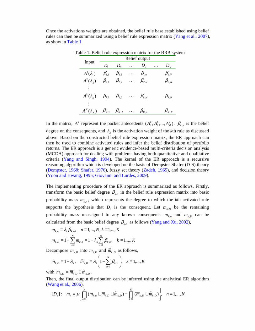
Fig. 5 Comparison between RM-WB and BRB with 3-asset-class portfolios

As shown in Fig. 5, the BRB system can closely replicate the non-linear relationship between asset weight combination and the mean and risk of portfolio returns. The maximum absolute deviation between RM-WB and BRB outputs is less than 0.2%. Using these interpolation points, we can get the approximated efficient frontier as shown in Fig. 6.

2.2 2.3 2.4 2.5 2.6 2.7 2.8 2.9 3 3.1 3.2

x 105

3.5

3.52

3.54

3.56

3.58

3.6

3.62

3.64

3.66

3.68x 10

5

Risk

Ret

urn

Rule points

Interpolation pointsEfficient frontier

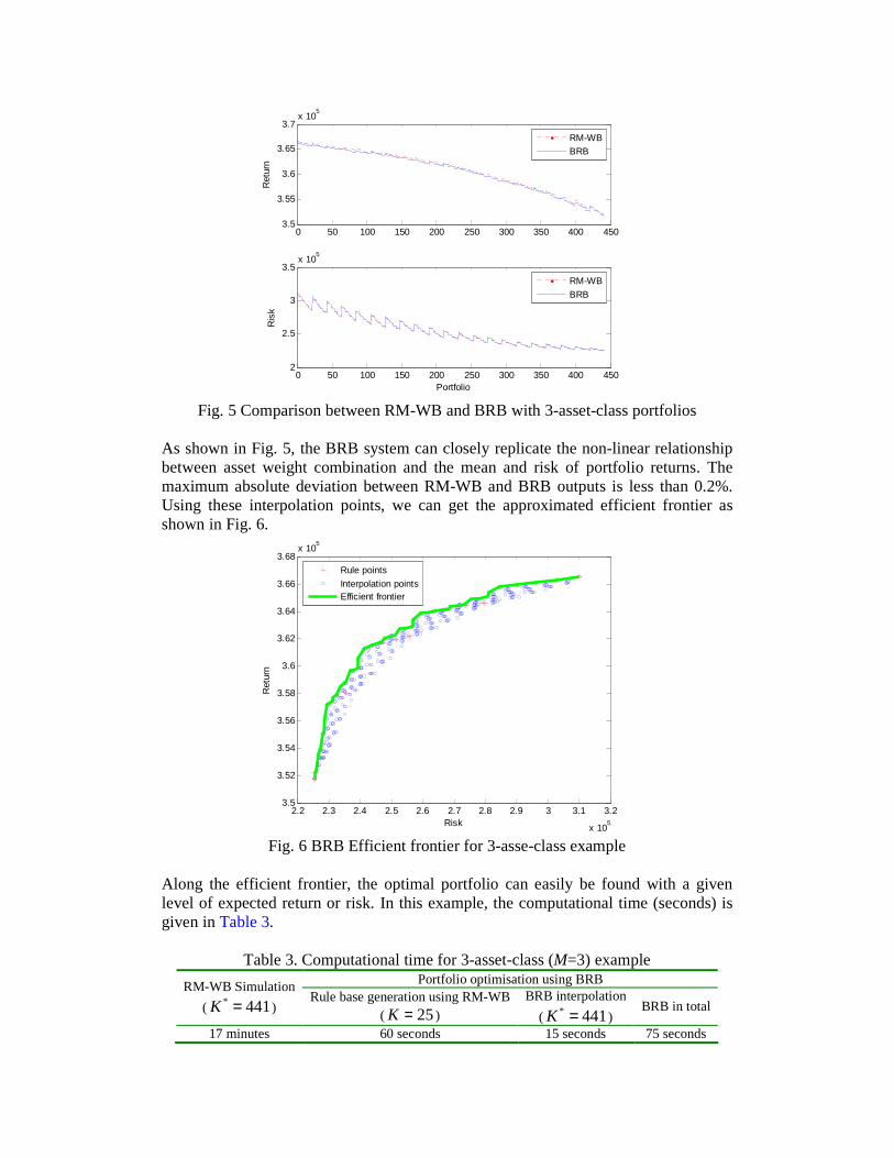
Fig. 6 BRB Efficient frontier for 3-asse-class example

Along the efficient frontier, the optimal portfolio can easily be found with a given level of expected return or risk. In this example, the computational time (seconds) is given in Table 3.

Table 3. Computational time for 3-asset-class (M=3) example Portfolio optimisation using BRB RM-WB Simulation

( 441* =K ) Rule base generation using RM-WB

( 25=K )

BRB interpolation

( 441* =K ) BRB in total

17 minutes 60 seconds 15 seconds 75 seconds

It is obvious that the BRB system studied in this paper is quite efficient for generating the efficient frontier.

4.2 Nine-asset-class application

This section solves 9-asset-class set which includes World equity (ex US), US large cap growth, US large cap value, US midcap, US smallcap, Cash, US bonds, US muni bonds, World bonds (ex US). The bounds are given in Table 4.

Table 4. Lower and upper bounds of 9 asset classes

World equity

(ex US)

US large cap

growth

US large cap

value

US mid cap

US small cap

Cash US

bonds

US muni bonds

World bonds

(ex US) lb 0 0.15 0 0 0.05 0 0.1 0 0.15 ub 0.2 0.45 0.21 0.17 0.25 0.9 0.25 0.2 0.45

In this case, the upper bound of Cash is updated to 0.55 at first according to the equations (5) and (6). The numbers of referential values for the first 81=−M asset classes are 2, 3, 2, 2, 2, 5, 2 and 2 respectively. Referential values are positioned evenly in the feasible interval of each asset weight. This leads to 960 initial weight combinations. As there are 874 points in infeasible space, 418 projected rule points are generated to construct an initial belief rule base with 504418874960 =+−=K referential rule points in total. The number of buckets used to group the consequential returns is 100=N . Further, we uniformly select 3, 3, 3, 2, 2, 7, 2 and 3 points from the feasible intervals of asset classes. Using the similar process of constructing rule points above,

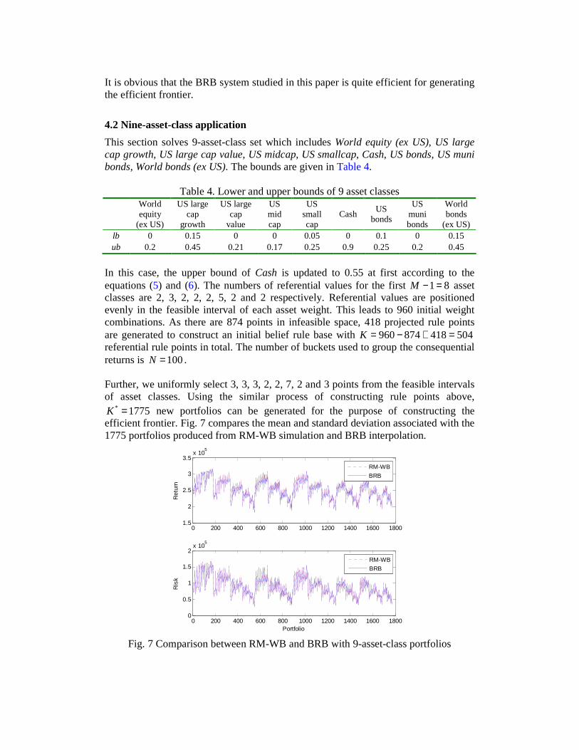
1775* =K new portfolios can be generated for the purpose of constructing the efficient frontier. Fig. 7 compares the mean and standard deviation associated with the 1775 portfolios produced from RM-WB simulation and BRB interpolation.

0 200 400 600 800 1000 1200 1400 1600 18001.5

2

2.5

3

3.5x 10

5

Ret

urn

RM-WB

BRB

0 200 400 600 800 1000 1200 1400 1600 18000

0.5

1

1.5

2x 10

5

Portfolio

Ris

k

RM-WB

BRB

Fig. 7 Comparison between RM-WB and BRB with 9-asset-class portfolios

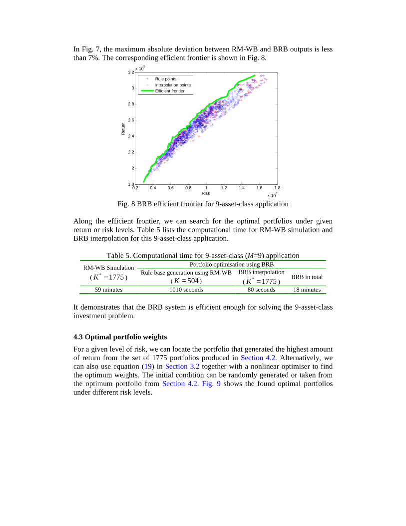
In Fig. 7, the maximum absolute deviation between RM-WB and BRB outputs is less than 7%. The corresponding efficient frontier is shown in Fig. 8.

0.2 0.4 0.6 0.8 1 1.2 1.4 1.6 1.8

x 105

1.8

2

2.2

2.4

2.6

2.8

3

3.2x 10

5

Risk

Ret

urn

Rule pointsInterpolation pointsEfficient frontier

Fig. 8 BRB efficient frontier for 9-asset-class application

Along the efficient frontier, we can search for the optimal portfolios under given return or risk levels. Table 5 lists the computational time for RM-WB simulation and BRB interpolation for this 9-asset-class application.

Table 5. Computational time for 9-asset-class (M=9) application Portfolio optimisation using BRB RM-WB Simulation

( 1775* =K ) Rule base generation using RM-WB

( 504=K )

BRB interpolation

( 1775* =K ) BRB in total

59 minutes 1010 seconds 80 seconds 18 minutes

It demonstrates that the BRB system is efficient enough for solving the 9-asset-class investment problem.

4.3 Optimal portfolio weights

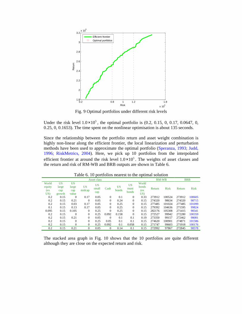
For a given level of risk, we can locate the portfolio that generated the highest amount of return from the set of 1775 portfolios produced in Section 4.2. Alternatively, we can also use equation (19) in Section 3.2 together with a nonlinear optimiser to find the optimum weights. The initial condition can be randomly generated or taken from the optimum portfolio from Section 4.2. Fig. 9 shows the found optimal portfolios under different risk levels.

0.2 0.8 1 1.2 1.8

x 105

1.8

2

2.2

2.4

2.6

2.8

3

3.2x 10

5

Risk

Ret

urn

Efficient frontier

Optimal portfolios

Fig. 9 Optimal portfolios under different risk levels

Under the risk level 5100.1 × , the optimal portfolio is (0.2, 0.15, 0, 0.17, 0.0647, 0, 0.25, 0, 0.1653). The time spent on the nonlinear optimisation is about 135 seconds. Since the relationship between the portfolio return and asset weight combination is highly non-linear along the efficient frontier, the local linearization and perturbation methods have been used to approximate the optimal portfolio (Speranza, 1993; Judd, 1996; RiskMetrics, 2004). Here, we pick up 10 portfolios from the interpolated efficient frontier at around the risk level 5100.1 × . The weights of asset classes and the return and risk of RM-WB and BRB outputs are shown in Table 6.

Table 6. 10 portfolios nearest to the optimal solution Asset class RM-WB BRB

World equity

(ex US)

US large cap

growth

US large cap

value

US midcap

US small cap

Cash US

bonds

US muni bonds

World bonds

(ex US)

Return Risk Return Risk

0.2 0.15 0 0.17 0.05 0 0.1 0 0.33 273912 100524 273912 100605 0.2 0.15 0.21 0 0.05 0 0.24 0 0.15 274320 98634 274320 98715 0.2 0.15 0.03 0.17 0.05 0 0.25 0 0.15 277485 101024 277485 101099 0.1 0.15 0.13 0.17 0.05 0 0.25 0 0.15 279392 104636 271595 99824

0.095 0.15 0.105 0 0.25 0 0.25 0 0.15 282176 105308 271415 98341 0.2 0.15 0 0 0.25 0.092 0.158 0 0.15 272527 99942 272280 100359 0.2 0.15 0.21 0 0.05 0 0.1 0.1 0.19 273350 99157 272462 98081 0.2 0.15 0 0 0.25 0.05 0.1 0.1 0.15 274620 100901 274871 101586 0.2 0.15 0 0 0.25 0.092 0.1 0.058 0.15 271747 99603 271918 100176 0.2 0.15 0.21 0 0.05 0 0.14 0.1 0.15 272992 97867 272845 98578

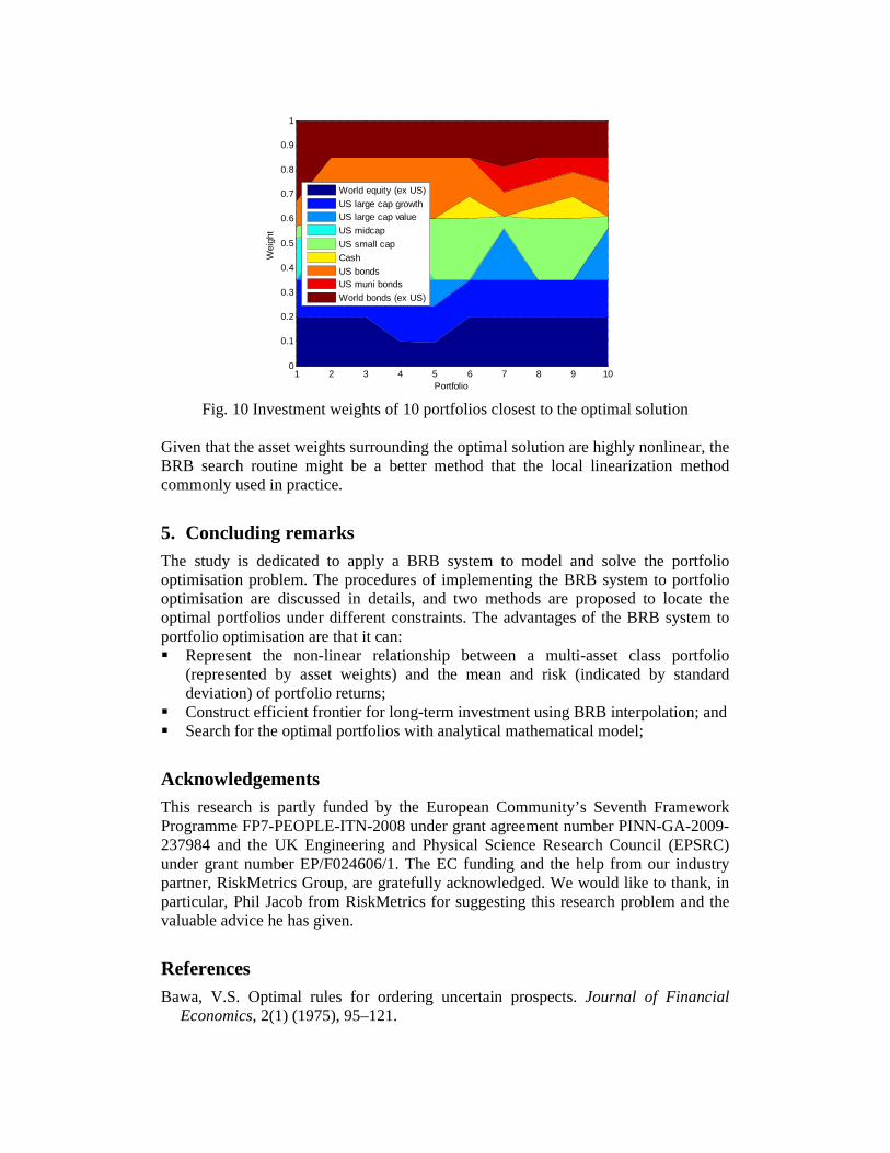
The stacked area graph in Fig. 10 shows that the 10 portfolios are quite different although they are close on the expected return and risk.

1 2 3 4 5 6 7 8 9 100

0.1

0.2

0.3

0.4

0.5

0.6

0.7

0.8

0.9

1

Portfolio

Wei

ght

World equity (ex US)

US large cap growthUS large cap value

US midcap

US small cap

Cash

US bondsUS muni bonds

World bonds (ex US)

Fig. 10 Investment weights of 10 portfolios closest to the optimal solution

Given that the asset weights surrounding the optimal solution are highly nonlinear, the BRB search routine might be a better method that the local linearization method commonly used in practice.

5. Concluding remarks The study is dedicated to apply a BRB system to model and solve the portfolio optimisation problem. The procedures of implementing the BRB system to portfolio optimisation are discussed in details, and two methods are proposed to locate the optimal portfolios under different constraints. The advantages of the BRB system to portfolio optimisation are that it can: � Represent the non-linear relationship between a multi-asset class portfolio

(represented by asset weights) and the mean and risk (indicated by standard deviation) of portfolio returns;

� Construct efficient frontier for long-term investment using BRB interpolation; and � Search for the optimal portfolios with analytical mathematical model;

Acknowledgements This research is partly funded by the European Community’s Seventh Framework Programme FP7-PEOPLE-ITN-2008 under grant agreement number PINN-GA-2009-237984 and the UK Engineering and Physical Science Research Council (EPSRC) under grant number EP/F024606/1. The EC funding and the help from our industry partner, RiskMetrics Group, are gratefully acknowledged. We would like to thank, in particular, Phil Jacob from RiskMetrics for suggesting this research problem and the valuable advice he has given.

References Bawa, V.S. Optimal rules for ordering uncertain prospects. Journal of Financial

Economics, 2(1) (1975), 95–121.

Bekkers N., R.Q. Doeswijk, T.W. Lam. Strategic Asset Allocation: Determining the Optimal Portfolio with Ten Asset Classes. Journal of Wealth Management, 12(3) (2009), 61–77.

Black, F., and R. Litterman. Global Portfolio Optimization. Financial Analysts Journal, 48(5) (1992), 28–43.

Brandt, M.W., A. Goyal, P. Santa-Clara, J.R. Stroud. A Simulation Approach to Dynamic Portfolio Choice with an Application to Learning About Return Predictability. Review of Financial Studies, 18(3) (2005), 831–873.

Brinson, G.P., L.R. Hood, and G.L. Beebower. Determinants of Portfolio Performance. Financial Analysts Journal, 42(4) (1986), 39–48.

Campbell, J.Y., L.M. Viceira. Strategic Asset Allocation: Portfolio Choice for Long-Term Investors. Oxford University Press, Oxford, UK. 2002.

Çelikyurta and S. Özekici. Multiperiod portfolio optimization models in stochastic markets using the mean–variance approach. European Journal of Operational Research, 179(1) (2007), 186–202.

Chen Y.W., Yang Jian-Bo, Dong-Ling Xu, Zhi-Jie Zhou, and Da-Wei Tang (in review). Inference analysis and adaptive training for belief rule based systems. Expert Systems with Applications, 2010.

Coleman T., Branch M.A., Grace A. Optimization Toolbox – For Use With MATLAB. Natick, MA: The Mathworks Inc. 1999.

Dempster A.P. A generalization of Bayesian inference. Journal of the Royal Statistical Society, Series B 30(2) (1968), 205–247.

Ehrgott, M., K. Klamroth, C. Schwehm. An MCDM approach to portfolio optimization. European Journal of Operational Research 155 (2004), 752–770.

Gaivoronski, A.A., G. Pflug. Value at Risk in Portfolio Optimization: Properties and Computational Approach. Journal of Risk, 7(2) (2005), 1–31.

Giovanni P., Lurdes I. Decision Theory: Principles and Approaches. John Wiley & Sons. 2009.

Glasserman, P. Monte Carlo Methods in Financial Engineering. Springer-Verlag, New York. 2004.

Gratcheva, E.M., and Falk J.E. Optimal deviations from an asset allocation. Computers & Operations Research, 30 (2003), 1643–1659.

Greer, R.J. What is an asset class, anyway? The Journal of Portfolio Management, 23(2) (1997), 86–91.

Hensel, C.R., D.D. Ezra, J.H. Ilkiw. The Importance of the Asset Allocation Decision. Financial Analysts Journal, 47(4) (1991), 65–72.

Ibbotson, R.G., P.D. Kaplan. Does Asset Allocation Policy Explain 40, 90, or 100 Percent of Performance? Financial Analysts Journal, 56(1) (2000), 26–33.

Idzorek, T. Developing Robust Asset Allocations. Working Paper, Ibbotson Associates, Chicago, 2006.

Jacobs B.I., K.N. Levy, H.M. Markowitz. Portfolio Optimization with Factors, Scenarios, and Realistic Short Positions. Operations Research, 53(4) (2005), 586–599.

Jorion, P. Bayesian and CAPM estimators of the means: Implications for portfolio selection. Journal of Banking & Finance, 15(3) (1991), 717–727.

Judd, K.L. Approximation, perturbation, and projection methods in economic analysis. In: Amman, H.M., Kendrick, D.A., Rust, J. (Eds.), Handbook of Computational Economics. North-Holland, Amsterdam, pp. 511–585 (Chapter 12). 1996.

Kan, R., G. Zhou. Optimal Portfolio Choice with Parameter Uncertainty. Journal of Financial and Quantitative Analysis, 42(3) (2007), 621–656.

Kim J.S., Y.C. Kim, K.Y. Shin. An Algorithm for Portfolio Optimization Problem, Informatica, 16(1) (2005) 93–106.

Koskosidis Y., Y.A., A.M. Duarte. A Scenario-Based Approach to Active Asset Allocation. The Journal of Portfolio Management, 23(2) (1997), 74–85.

Kritzman, M. Toward Defining an Asset Class. The Journal of Alternative Investments, 2(1) (1999), 79–82.

Markowitz, H., Portfolio Selection. The Journal of Finance, 7(1) (1952), 77–91. Markowitz, H.M., A.F. Perold. Portfolio Analysis with Factors and Scenarios. The

Journal of Finance, 36(4) (1981), 871–877. Palmquist, J., P. Krokhmal, S. Uryasev. Portfolio optimization with conditional value-

at-risk objective and constraints. Journal of Risk, 4(2) (2001), 21–41. RiskMetrics, Risk Management: A Practical Guide. RiskMetrics Group. August 1999. RiskMetrics, WealthBench Technical Document, Preliminary Client Version,

RiskMetrics Group. January, 2004. Shafer G. Mathematical Theory of Evidence. Princeton, NJ: Princeton University

Press. 1976. Speranza, M.G. Linear programming models for portfolio optimization, Finance, 14

(1993), 107–123. Tütüncü, R.H., M. Koenig. Robust asset allocation. Annals of Operations Research,

132 (2004), 157–187. Wang Y.M., Yang J.B., Xu D.L. Environmental Impact Assessment Using the

Evidential Reasoning Approach. European Journal of Operational Research, 174(3) (2006), 1885–1913.

Xu D.L., Liu J., Yang J.B., Liu G.P., Wang J., Jenkinson I., Ren J. Inference and learning methodology of belief-rule-based expert system for pipeline leak detection. Expert Systems with Applications 32(1) (2007), 103–113.

Yang J.B., Singh M.G. An evidential reasoning approach for multiple attribute decision making with uncertainty. IEEE Transactions on Systems, Man, and Cybernetics 24(1) (1994), 1–18.

Yang J.B., Liu J., Wang J., Sii H.S., Wang H.W. A belief rule-base inference methodology using the evidential reasoning approach – RIMER. IEEE Transactions on Systems, Man, and Cybernetics – Part A, 36(2) (2006), 266–285.

Yang J.B., Liu J., Xu D.L., Wang J., Wang H.W. Optimization models for training belief rule based systems. IEEE Transactions on Systems, Man, and Cybernetics – Part A 37(4) (2007), 569–585.

Yang J.B., Xu D.L. On the evidential reasoning algorithm for multiattribute decision analysis under uncertainty. IEEE Transactions on Systems, Man, and Cybernetics - Part A: Systems and Humans 32(3) (2002), 289–304.

Yoon K., Hwang C.L. Multiple Attribute Decision Making: An Introduction. Thousand Oaks, CA: Sage Publications. 1995.

Zadeh L.Z. Fuzzy sets. Information Control 8(3) (1965), 338–353. Zhou Z.J., Hu C.H., Yang J.B., Xu D.L., Zhou D.H. Online updating belief-rule-based

system for pipeline leak detection under expert intervention. Expert Systems with Applications 36 (2009), 7700–7709.