Multi-arm trials: a comparison of multi-arm multi-stagedesigns and adaptive randomisation

James WasonMRC Biostatistics Unit Hub for Trials Methodology Research

Cambridge, UKjames.wason@mrc-bsu.cam.ac.uk

Joint work with Lorenzo Trippa, Dana-Farber Cancer Institute, Boston.

Overview

Multi-arm trials.

Multi-arm multi-stage designs.

Adaptive randomisation.

Comparison of designs for neo-adjuvant breast cancer trial.

Conclusions.

Introduction - multi-arm trials

In some therapeutic areas, there may be several possible agents/treatmentsawaiting trials.

The traditional approach is to test each one by one in separate controlledclinical trials.

An alternative is one trial in which several novel treatments are compared.Advantages:

Efficient and cheaper, since a shared control group is used.

More treatments can be tested with a limited set of patients.

More popular with patients as a greater chance of being allocated to a newtreatment.

Multi-arm trials

Multi-arm trials

Potential sample size reductions depends on number of experimental arms(call this K ), and whether we want to adjust for multiple testing.

Multiple testing because there are now several null hypotheses being tested.

If multiple testing is considered important, then we wish to control thefamily-wise error rate (FWER), which is the probability of rejecting any truenull hypothesis.

Otherwise just control the per-comparison type-I error rate - probability ofrejecting a true null hypothesis.

Multi-arm trials

For example, for a controlled phase II trial with a total of 100 patients:

Number ex-perimentaltreatments

Sample size(separate)

Sample size(multi-arm, noadjustment)

Sample size(multi-arm, fulladjustment)

2 200 150 1803 300 200 2564 400 250 3355 500 300 420

Multi-arm trials with interim analyses

Can also add interim analyses to a multi-arm trial.

Interim analyses allow changes to be made to the trial using data gatheredduring the trial.

For example, if a treatment has performed poorly, might want to drop it fromthe trial or assign fewer patients to it.

Could also allow trial to stop if an effective treatment is found (notconsidered in this talk).

Having interim analyses generally increases the efficiency and ethics of a trial.

But there are different ways to make use of interim information.

Approach 1: MAMS designs

One approach is to set stopping boundaries, which the test statistics arecompared to at each analysis.

This approach is a generalisation of group-sequential designs to multi-armtrials.

Has been applied in several real trials including STAMPEDE and TAILoR.

Methodology fairly well researched for normally distributed and survivalendpoints.

Approach 1: MAMS designs−1

01

23

Analysis number

Test

sta

tistic

1 2 3

Approach 1: MAMS designs−1

01

23

Analysis number

Test

sta

tistic

1 2 3

Approach 1: MAMS designs−1

01

23

Analysis number

Test

sta

tistic

1 2 3

Approach 1: MAMS designs−1

01

23

Analysis number

Test

sta

tistic

1 2 3

Approach 1: MAMS designs−1

01

23

Analysis number

Test

sta

tistic

1 2 3

Approach 1: MAMS designs−1

01

23

Analysis number

Test

sta

tistic

1 2 3

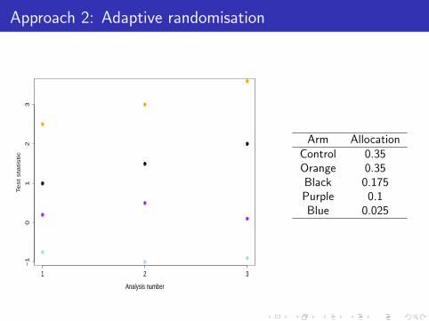
Approach 2: Adaptive randomisation

A second approach is called adaptive randomisation (AR).

AR is a procedure that increases the allocation for treatments that have beensuccessful and decreases it for treatments that have been unsuccessful.

Has been extensively researched for the case of a single experimentaltreatment.

In this case, it leads to deviations from the most powerful 1:1 allocation.

This means it loses power, but tends to result in better patient outcomes inthe trial.

Approach 2: Adaptive randomisation

If AR is applied in a multi-arm trial, one can protect the allocation to thecontrol group. (Trippa et al, 2012)

Basically this means AR is just applied amongst the experimental treatments,and the allocation to controls is set independently.

For example, allocation to controls could be set so that number of controls =number of patients on most effective experimental arm.

This means that the power of the trial is protected, but ineffectiveexperimental arms can be assigned fewer patients.

Can be thought of as a more flexible version of the MAMS approach.

Approach 2: Adaptive randomisation−

10

12

3

Analysis number

Te

st

sta

tistic

1 2 3

Arm AllocationControl 0.2Orange 0.2Black 0.2Purple 0.2Blue 0.2

Approach 2: Adaptive randomisation−

10

12

3

Analysis number

Te

st

sta

tistic

1 2 3

Arm AllocationControl 0.3Orange 0.3Black 0.2Purple 0.15Blue 0.05

Approach 2: Adaptive randomisation−

10

12

3

Analysis number

Te

st

sta

tistic

1 2 3

Arm AllocationControl 0.35Orange 0.35Black 0.175Purple 0.1Blue 0.025

Approach 2: Adaptive randomisation−

10

12

3

Analysis number

Te

st

sta

tistic

1 2 3

Arm AllocationControl 0.35Orange 0.35Black 0.175Purple 0.1Blue 0.025

Comparison of designs

More formal descriptions of designs in submitted paper (available uponrequest).

Also descriptions of procedures to find design with given type-I errorrate/FWER and power.

We compared the designs on a wide-range of scenarios as well as on a realtrial.

Comparison of designs

Both methods controlled the type-I error / FWER.

Generally if all treatments were ineffective, then MAMS design had a lowerexpected sample size than the (fixed) sample size used by AR.

We investigated adding a futility rule to AR, which helped narrow the gap.

However, in the situation where there was an effective experimentaltreatment, AR required a lower sample size for the same power.

AR also led to a slightly better average treatment response.

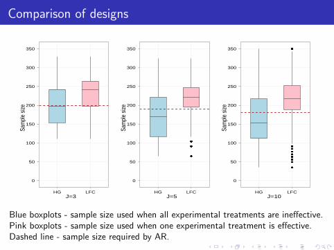
Next slide shows sample size requirements for 80% power at 20% FWER todetect difference of 0.2 in success probability.

Comparison of designs

J=3

Sam

ple

size

0

50

100

150

200

250

300

350

HG LFCJ=5

Sam

ple

size

0

50

100

150

200

250

300

350

HG LFCJ=10

Sam

ple

size

0

50

100

150

200

250

300

350

HG LFC

Blue boxplots - sample size used when all experimental treatments are ineffective.Pink boxplots - sample size used when one experimental treatment is effective.Dashed line - sample size required by AR.

Case-study

As a case-study we used the NeoSphere trial, which was a multi-arm trialwith three experimental arms and a control arm.

Approximately 400 patients were recruited into the trial, equally allocatedbetween the four arms.

Endpoint is pathological complete response (pCR), a binary endpoint.

Case-study - delay between recruitment and assessment

An important issue in the efficiency of adaptive designs is delay betweenrecruiting patients and assessing them.

Adaptive designs will be less efficient if the delay is long and/or therecruitment rate is high.

This is because at an interim analysis there will be patients who have beenrecruited but not yet assessed. They will not contribute to that analysis, orany analysis if the arm is dropped.

The Neosphere trial had an average recruitment rate of 4 patients per weekand a delay of 15 weeks.

We investigated the performance of the AR and MAMS designs when therewas 15 weeks delay and the recruitment rate was 2, 4 and 8 per week.

Maximum sample size of AR and expected sample size of MAMS set to 400.

Case-study

J Recruitment/week

Power ESS-HG ESS-LFC

AR MAMS AR MAMS AR MAMS

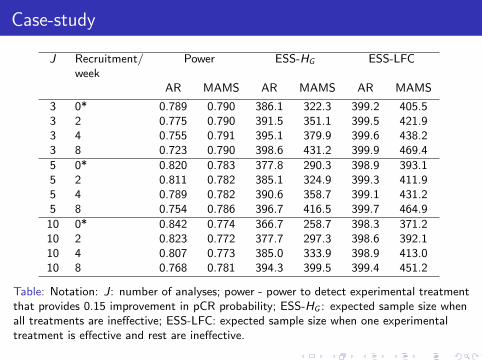
3 0* 0.789 0.790 386.1 322.3 399.2 405.53 2 0.775 0.790 391.5 351.1 399.5 421.93 4 0.755 0.791 395.1 379.9 399.6 438.23 8 0.723 0.790 398.6 431.2 399.9 469.4

5 0* 0.820 0.783 377.8 290.3 398.9 393.15 2 0.811 0.782 385.1 324.9 399.3 411.95 4 0.789 0.782 390.6 358.7 399.1 431.25 8 0.754 0.786 396.7 416.5 399.7 464.9

10 0* 0.842 0.774 366.7 258.7 398.3 371.210 2 0.823 0.772 377.7 297.3 398.6 392.110 4 0.807 0.773 385.0 333.9 398.9 413.010 8 0.768 0.781 394.3 399.5 399.4 451.2

Table: Notation: J: number of analyses; power - power to detect experimental treatmentthat provides 0.15 improvement in pCR probability; ESS-HG : expected sample size whenall treatments are ineffective; ESS-LFC: expected sample size when one experimentaltreatment is effective and rest are ineffective.

Case-study

For comparison, power of multi-arm design without interim analyses is 0.707.

Delay has an effect on the efficiency of the two approaches.

As recruitment rate increases, power of AR falls, expected sample size ofMAMS increases.

More adjustment required for MAMS designs, otherwise operatingcharacteristics are much different to planned.

Interim analyses could be conducted after a given number of patients areassessed rather than recruited.

Alternatively some adjustment could be made to the boundaries.

Conclusions

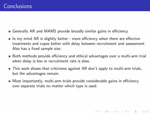
Generally AR and MAMS provide broadly similar gains in efficiency.

In my mind AR is slightly better - more efficiency when there are effectivetreatments and copes better with delay between recruitment and assessment.Also has a fixed sample size.

Both methods provide efficiency and ethical advantages over a multi-arm trialwhen delay is low or recruitment rate is slow.

This work shows that criticisms against AR don’t apply to multi-arm trials,but the advantages remain.

Most importantly, multi-arm trials provide considerable gains in efficiencyover separate trials no matter which type is used.

Formal description of MAMS designs

More formally, let there be J analyses.

Define futility boundaries, (f1, . . . , fJ) and group-size, n, number of patientsrecruited to each arm at each stage.

Calculate test statistic at stage j comparing effect of arm k to control group,call this Zjk .

If Zjk is below fj , drop arm k for futility.

If all arms have been stopped for futility, stop trial.

At final analysis, reject H(k)0 if ZJk > fJ .

Choose group-size and futility boundaries such that type-I error rate orFWER is controlled and power is equal to some specified level.

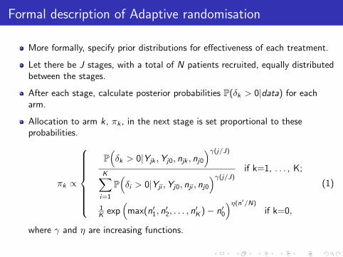
Formal description of Adaptive randomisation

More formally, specify prior distributions for effectiveness of each treatment.

Let there be J stages, with a total of N patients recruited, equally distributedbetween the stages.

After each stage, calculate posterior probabilities P(δk > 0|data) for eacharm.

Allocation to arm k, πk , in the next stage is set proportional to theseprobabilities.

πk ∝

P(δk > 0|Yjk ,Yj0, njk , nj0

)γ(j/J)

K∑i=1

P(δi > 0|Yji ,Yj0, nji , nj0

)γ(j/J)if k=1, . . . , K;

1K exp

(max(n′

1, n′2, . . . , n

′K )− n′

0

)η(n′/N)

if k=0,

(1)

where γ and η are increasing functions.

Formal description of Adaptive randomisation

At the end of the trial, test statistics for the effect of each arm againstcontrol, (Z1, . . . ,ZK ) are calculated.

If Zk is above a critical value c , then reject H(k)0 .

N and c are chosen to control the FWER/type-I error rate and power of thedesign.

The choice of γ() affects the efficiency of the design substantially.

We have explored a large number of possibilities and found the most efficientchoice (results in submitted paper, available upon request).