Tampere University of Technology Author(s) Müller, Juliane; Piché Robert

Title Mixture surrogate models based on Dempster-Shafer theory for global optimization problems Citation Müller, Juliane; Piché, Robert 2011. Mixture surrogate models based on Dempster- Shafer theory for global optimization problems. Journal of Global Optimization vol. 51, num. 1, 79-104. Year 2011 DOI http://dx.doi.org/10.1007/s10898-010-9620-y Version Post-print URN http://URN.fi/URN:NBN:fi:tty-201311011411 Copyright The final publication is available at link.springer.com.

All material supplied via TUT DPub is protected by copyright and other intellectual property rights, and duplication or sale of all or part of any of the repository collections is not permitted, except that material may be duplicated by you for your research use or educational purposes in electronic or print form. You must obtain permission for any other use. Electronic or print copies may not be offered, whether for sale or otherwise to anyone who is not an authorized user.

Mixture Surrogate Models Based on Dempster-Shafer Theory

for Global Optimization Problems

Juliane Muller · Robert Piche

Abstract Recent research in algorithms for solving global optimization problems using response surface

methodology has shown that it is in general not possible to use one surrogate model for solving different kinds

of problems. In this paper the approach of applying Dempster-Shafer theory to surrogate model selection and

their combination is described. Various conflict redistribution rules have been examined with respect to their

influence on the results. Furthermore, the implications of the surrogate model type, i.e. using combined, single

or a hybrid of both, have been studied. The suggested algorithms were applied to several well-known global

optimization test problems. The results indicate that the used approach leads for all problems to a thorough

exploration of the variable domain, i.e. the vicinities of global optima could be detected, and that the global

minima could in most cases be approximated with high accuracy.

Keywords Global optimization, Mixture surrogate models, Dempster-Shafer theory, Response surface

1 Introduction

The development and optimization of new products and engineering designs requires computationally

expensive simulations due to the complexity of the underlying processes. In order to obtain the response of

the system at one point it might be necessary to solve large systems of differential equations or to do some

other time consuming numerical simulations. Thus, using these simulation models during the optimization

process will lead to prohibitively high computation times as commonly used optimization routines require

many function evaluations. Furthermore, these optimization routines usually converge to a local optimum

close to the chosen starting point.

Surrogate models have been developed in order to reduce the necessary number of costly simulations while

searching for the global optimum of the problem at hand. The advantage of surrogate models is their low

computational complexity compared to the true simulation model. In general, a surrogate model can be

represented by

f(x) = s(x) + ǫ,

where f(x) denotes the output of the simulation model (also referred to as true model) at the point x, s(x)

denotes the output of the surrogate model, and ǫ represents the error between both.

Surrogate models can be either non-interpolating or interpolating [11]. Non-interpolating models include

for example polynomial regression models [20] and multivariate adaptive regression splines [6]. Radial basis

functions [2, 9, 22, 24, 25] and Kriging [12, 13, 17, 18] are interpolating surrogate models.

J. MullerTampere University of Technology, Department of MathematicsP.O. Box 553, FI-33101 Tampere, FinlandE-mail: juliane.mueller@tut.fi

R. PicheTampere University of Technology, Department of MathematicsP.O. Box 553, FI-33101 Tampere, FinlandE-mail: robert.piche@tut.fi

Surrogate models have for example been used by [7] during the optimization of helicopter rotor blades,

or also by [23] who designed a liquid-rocket injector with respect to multiple objectives. Efficient Global

Optimization (EGO) has been applied by [19] in order to optimize the shape of horn-loaded loudspeakers.

Surrogate models have also been used in automotive design (see for example [14, 30, 32]).

However, as shown for example by [8] and [28], one surrogate model does not suit all kinds of problems, i.e. a

certain surrogate model might perform very well on some problem type, but badly for other problems. If it is

not known beforehand which surrogate model is the most suitable for the problem at hand, different models

or also mixture models have to be tried in order to find the most effective one. Then, the challenge is the

determination of the best surrogate model and the adjustment of the influence of single surrogate models in

mixtures, respectively. The prediction y(x) of such a mixture surrogate model can in general be represented

as

y(x) =N

X

i=1

wiyi(x),N

X

i=1

wi = 1, (1)

where yi(x) denotes the prediction of the ith contributing model, wi ≥ 0 is the corresponding weight, and N

is the number of models.

Goel et al. [8] suggested different approaches for determining the weights of models in combinations.

However, only one of the approaches allows emphasizing and restricting the influence of good and bad model

characteristics, respectively. Moreover, in this approach parameters that are in general unknown must be

adjusted beforehand. Viana and Haftka [28] also considered mixture surrogate models and suggested the

optimization of an auxiliary function in order to obtain an approximation matrix. This matrix is in turn

used for determining the model weights, but it can lead to negative weights and weights larger than one, and

thus results may become inaccurate.

In order to overcome the mentioned problems the choice and combination of different surrogate models

via Dempster-Shafer theory [4, 26] will be considered in this paper. Dempster-Shafer theory (DST) is a

mathematical theory of evidence which provides means of combining information from different sources

in order to construct a degree of belief. The theory allows the combination of imprecise and uncertain

pieces of information which may even be conflicting. So-called basic probability assignments (BPA) contain

information about certain hypotheses (focal elements) and are combined in order to calculate the credibility

of a given hypothesis. Three functions are usually associated with BPAs, namely the belief (Bel), plausibility

(Pl) and pignistic probability (BetP) function.

In terms of surrogate models the BPAs can be, for example, model characteristics such as correlation

coefficients and root mean squared errors (RMSE). It is possible that one surrogate model has conflicting

characteristics, i.e. good (e.g. high correlation coefficients) and bad (e.g. high RMSE) characteristics.

This conflict must be considered when calculating the belief one has in the given model. Several conflict

redistribution rules have been developed in the literature. Dempster’s rule of combination redistributes the

conflict amongst all focal elements, regardless of which elements caused the conflict. However, as shown

by [31], the results of this approach may be counter-intuitive. Other ways of distributing the conflict in a

fairer way have been developed: the conflict can be assigned to the set reflecting complete ignorance [29],

or one may apply the proportional conflict redistribution (PCR) rules [27] to redistribute the conflict

among those focal elements that cause the conflict. The disadvantage of the latter approach is however the

computational complexity which increases with the number of information sources. Inagaki [10] proposes

a general formulation for the redistribution of the conflict incorporating parameters which in turn may

influence the result of the information combination.

The goal of this paper is to apply Dempster-Shafer theory in order to choose amongst different surrogate

models the most suitable one for a given optimization problem, and to find the weights of single models

contributing to combinations, respectively. It is necessary to guarantee a thorough global and local exploration

of the variable domain. Regions where the global optimum may be located must be examined thoroughly, but

the algorithm must also not get stuck in a local optimum. Since it is in general unknown whether mixture

models will be more successful than single models, the following alternative strategies shall be examined:

1. using the best mixture model for the first optimization steps, then switching to using always the best

single surrogate model,

2. using only the best mixture model,

3. using only the best single surrogate model.

2

The remainder of this paper is organized as follows. The considered surrogate models are briefly described in

Section 2. A description of the algorithm is given in Section 3, and the results for different test problems are

given in Section 4. Section 5 concludes the paper and future research topics are outlined.

2 Surrogate Models

In the following it is assumed that the true function f : Rk 7→ R has been sampled at n points of the domain

according to some given experimental design. Denote those sample sites by x1,x2, . . . ,xn, xi ∈ Rk ∀i, and

the corresponding function values by y1, y2, . . . , yn. Based on the given experimental design surrogate models

are built. The considered model types will be described next.

Polynomial regression models of different degrees can be easily built using the method of least squares. In

general, models of degree two are in most cases sufficient. The inclusion of cross terms is in many applica-

tion problems important since they reflect the interaction between different variables. Thus, considered are

polynomial regression models of second order which can be represented by

yi(xi) = β0 +k

X

j=1

βjxij +k

X

j=1

βjjx2ij +

kX

j1=1

kX

j2=1

j2 6=j1

βj1j2xi,j1xi,j2 + ǫi, i = 1, 2, . . . , n,

where βi, i = 0, . . . , n, are parameters to be determined.

Multivariate adaptive regression splines (MARS) is a non-parametric regression technique introduced by [6].

The method can be interpreted as an extension of linear models to include non-linearities and interactions.

In general MARS models are of the form

y(x) =

mX

i=1

aiBi(x),

where ai are constant coefficients, and Bi(x) are basis functions. Basis functions can either be just a constant,

i.e. the intercept, a hinge function of the form max {0, x − const} or max {0, const − x}, or the product of

two or more hinge functions representing interactions between variables. The MARS model is built in two

phases, namely a forward and backward iterative approach, where the basis functions are adaptively selected

in order to approximate the true function.

Radial basis functions have been introduced by [5] and with their help the curvature of the true function can

be modeled well. The surrogate model is defined by

y(x) =n

X

i=1

λiφ`

‖x − xi‖2

´

+ p(x), (2)

where ‖ · ‖ denotes the Euclidean norm, λ1, λ2, . . . , λn ∈ R, φ : R+ 7→ R are radial basis functions, and p(x)

denotes an optional polynomial tail of the form b′x+a, b ∈ Rk, a ∈ R. Frequently used radial basis functions

are, for example, cubic, thin plate spline, Gaussian, multiquadric, and inverse-multiquadric. The required

parameters are determined by solving the linear system

»

Φ P

P′ 0

– »

λ

c

–

=

»

F

0

–

, where P =

2

6

6

6

4

x′1 1

x′2 1...

...

x′n 1

3

7

7

7

5

, λ =

2

6

6

6

4

λ1

λ2

...

λn

3

7

7

7

5

c =

2

6

6

6

6

6

6

4

b1b2...

bk

a

3

7

7

7

7

7

7

5

, F =

2

6

6

6

4

y1

y2

...

yn

3

7

7

7

5

,

and Φ is an n × n matrix with entries Φij = φ`

‚

‚xi − xj

‚

‚

2

´

. Then, if rank(P )= k+1, the matrix

»

Φ P

P′ 0

–

is nonsingular and the linear system has a unique solution [21]. Therefore, it is possible to obtain a unique

radial basis function interpolant to the true function f .

Kriging was developed by the French mathematician Georges Matheron [18] and was first used in numerical

experiments in 1988 [3]. Kriging models consist of two components. The first component is some simple model

3

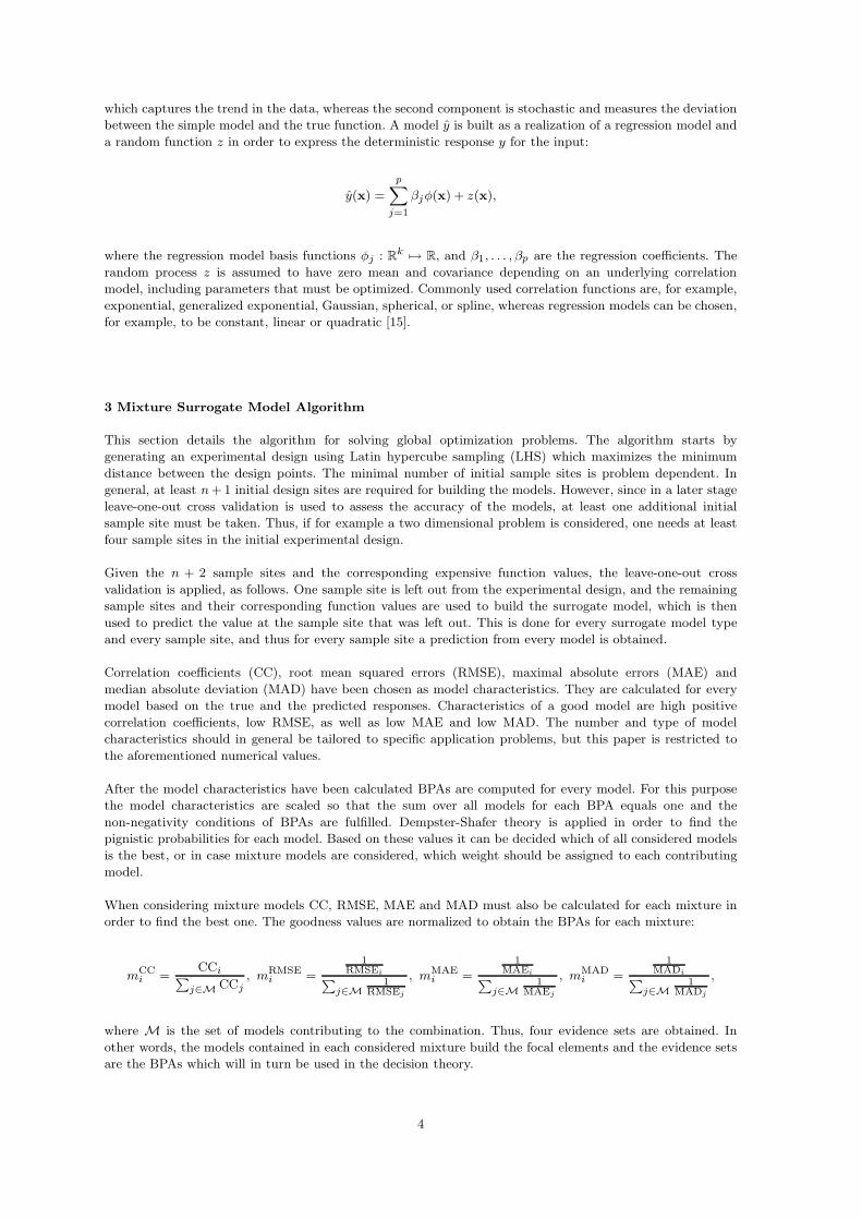
which captures the trend in the data, whereas the second component is stochastic and measures the deviation

between the simple model and the true function. A model y is built as a realization of a regression model and

a random function z in order to express the deterministic response y for the input:

y(x) =

pX

j=1

βjφ(x) + z(x),

where the regression model basis functions φj : Rk 7→ R, and β1, . . . , βp are the regression coefficients. The

random process z is assumed to have zero mean and covariance depending on an underlying correlation

model, including parameters that must be optimized. Commonly used correlation functions are, for example,

exponential, generalized exponential, Gaussian, spherical, or spline, whereas regression models can be chosen,

for example, to be constant, linear or quadratic [15].

3 Mixture Surrogate Model Algorithm

This section details the algorithm for solving global optimization problems. The algorithm starts by

generating an experimental design using Latin hypercube sampling (LHS) which maximizes the minimum

distance between the design points. The minimal number of initial sample sites is problem dependent. In

general, at least n + 1 initial design sites are required for building the models. However, since in a later stage

leave-one-out cross validation is used to assess the accuracy of the models, at least one additional initial

sample site must be taken. Thus, if for example a two dimensional problem is considered, one needs at least

four sample sites in the initial experimental design.

Given the n + 2 sample sites and the corresponding expensive function values, the leave-one-out cross

validation is applied, as follows. One sample site is left out from the experimental design, and the remaining

sample sites and their corresponding function values are used to build the surrogate model, which is then

used to predict the value at the sample site that was left out. This is done for every surrogate model type

and every sample site, and thus for every sample site a prediction from every model is obtained.

Correlation coefficients (CC), root mean squared errors (RMSE), maximal absolute errors (MAE) and

median absolute deviation (MAD) have been chosen as model characteristics. They are calculated for every

model based on the true and the predicted responses. Characteristics of a good model are high positive

correlation coefficients, low RMSE, as well as low MAE and low MAD. The number and type of model

characteristics should in general be tailored to specific application problems, but this paper is restricted to

the aforementioned numerical values.

After the model characteristics have been calculated BPAs are computed for every model. For this purpose

the model characteristics are scaled so that the sum over all models for each BPA equals one and the

non-negativity conditions of BPAs are fulfilled. Dempster-Shafer theory is applied in order to find the

pignistic probabilities for each model. Based on these values it can be decided which of all considered models

is the best, or in case mixture models are considered, which weight should be assigned to each contributing

model.

When considering mixture models CC, RMSE, MAE and MAD must also be calculated for each mixture in

order to find the best one. The goodness values are normalized to obtain the BPAs for each mixture:

mCCi =

CCiP

j∈M CCj, mRMSE

i =

1RMSEi

P

j∈M1

RMSEj

, mMAEi =

1MAEi

P

j∈M1

MAEj

, mMADi =

1MADi

P

j∈M1

MADj

,

where M is the set of models contributing to the combination. Thus, four evidence sets are obtained. In

other words, the models contained in each considered mixture build the focal elements and the evidence sets

are the BPAs which will in turn be used in the decision theory.

4

In order to illustrate the above procedure consider the following example. Assume the four models described

in Section 2 are available and denote the polynomial model by P, the RBF model by R, the Kriging model by

K, and the MARS model by M. After cross-validation the characteristics of the single models are as follows:

mCCP = 0.29, mCC

R = 0.29, mCCK = 0.42, mCC

M = 0

mRMSEP = 0.11, mRMSE

R = 0.24, mRMSEK = 0.25, mRMSE

M = 0.40,

mMAEP = 0.10, mMAE

R = 0.24, mMAEK = 0.25, mMAE

M = 0.41,

mMADP = 0.17, mMAD

R = 0.27, mMADK = 0.26, mMAD

M = 0.30.

After applying DST the pignistic probabilities of the models are

BetP(P) = 0.05, BetP(R) = 0.40, BetP(K) = 0.55, BetP(M) = 0,

and thus, if a single model was used in the next step, the Kriging model would be chosen. If however a mixture

model is required, the given pignistic probabilities are used for calculating the weights of the contributing

models. Assume that models P and R are supposed to be combined. Then the weights for both models are

wP =BetP(P)

BetP(P) + BetP(R), wR =

BetP(R)

BetP(P) + BetP(R),

respectively. Thus wP + wR = 1, and these weights are used to build the model estimate according to (1):

y(x) = wPyP(x) + wRyR(x),

where yP(x) and yR(x) are the predictions of the polynomial and RBF model at the point x, respectively.

The algorithm considers every possible (one-,) two-, three- and four-model mixture, and therefore the focal

elements to be considered are {P}, {R}, {K}, and {M} for the single models, {P,R}, {P,K}, {P,M}, {R,K},

{R,M}, and {K,M} for the two-model combinations, {P,R,K}, {P,R,M},{P,K,M}, and {R,K,M} for the

three-model combinations, and {P,R,K,M} for the four-model combination. In case of mixture models BPAs

must be calculated based on the cross validation characteristics of the corresponding mixture.

In the next step, one of the described conflict redistribution rules from Section 1 is applied, i.e. the evidences

obtained are combined, and for each mixture and single model the corresponding belief, plausibility and

pignistic probability is calculated. Then the (mixture) model with the highest plausibility value is chosen as

new response surface1.

Next a new sample site must be chosen. The algorithm must guarantee a thorough local as well as a global

search, i.e. the algorithm should be able to find objective function valleys and sample there several times, but

must also be prevented from getting stuck in a local optimum. The difficulty is to decide when to interrupt

the local search, i.e. after how many samples in a certain region the search should continue in a more global

manner and vice versa.

If sites of the minima of the single models contributing to the mixture model are very distant from each

other, it might be an indication that there are several regions in the variable domain where local or global

optima could be located, and thus sampling at these points may be favorable. However, if the sites are close

together, this approach may lead to a very local search.

In order to prevent the algorithm from excessive sampling in the vicinity of the currently best point it is

necessary to force the search away from regions where already many samples have been taken. For this

purpose the minimal distances dmin between every newly added sample site and all other already sampled

points are recorded, and in case a certain amount of sample sites closer to each other than some predefined

threshold distance d∗ is exceeded, the algorithm must be prevented from adding more points in the already

densely sampled region. The smaller the number of allowed close points is, the more global the search

becomes. On the other hand, increasing the maximal allowed number of close samples leads to a longer

local search which adds more sample points in the vicinity of the currently best known point. Similarly, the

smaller the threshold distance d∗, the more thorough the local search becomes.

1 Note that the combination of all models, i.e. the universal set, always has plausibility and belief values of one, andmust thus be considered separately.

5

The sample sites where the true function has already been evaluated are clustered according to a k-means

algorithm [16], where the number of clusters k is determined dynamically. If a large cluster has been found,

a densely-sampled area is defined based on the cluster’s content. Denote Xck =ˆ

xck,1,xck,2, . . . ,xck,k

˜′the

matrix of sample sites contained in the considered cluster ck, where xck,i are column vectors. Lower bounds

[minXck (:, i1) , . . . , minXck(:, ik)] and upper bounds [maxXck(:, i1), . . . , maxXck(:, ik)] are defined for the

variables i1, . . . , ik ∈ {1, 2, . . . , k} that are closest to each other, and thus determine the boundary of the

densely-sampled area. Note that these bounds do not exist for all variables. This issue is important especially

when problems with very long and steep valleys are considered. In such cases it is of advantage to not define

bounds on all variables.

When searching for new prospective regions that may contain local or global optima a target value strategy

similar to the one proposed by Jones [11] is applied. A vector T = smin −α (fmax − fmin) represents desired

function values, where α is a vector of non-negative scalars (see also [9]). smin stands for the minimum of the

response surface, and fmin and fmax denote, respectively, the minimal and maximal function value obtained

so far.

An optimization routine is applied in order to minimize an auxiliary function that represents the difference

between the target values Ti and the prediction of the response surface. In order to search more globally a

penalty term is used to prevent the search from entering the densely-sampled area. Similarly, in the local

search a penalty term is used to prevent the search from leaving the densely-sampled area. In this way the

search can be drawn away from or restricted to the already thoroughly examined area.

For each target the point where the minimum has been located is recorded. These points are clustered into k

groups where k can be varied in order to increase or decrease the amount of desired new sample sites. From

each of the k groups only the representative that reached the lowest value while optimizing the auxiliary

function is chosen as new sample site. Problems arise however if the global optimum is inside (global search)

or outside (local search) the densely-sampled region. This problem is addressed by setting the penalty of a

point that reaches during the optimization of the auxiliary function a much better function value than any

other candidate to zero.

The calculation of the minimum of the response surface and of the auxiliary function require themselves

optimization routines. Two different approaches have been compared, namely a Hooke-Jeeves pattern search

method and the accelerated random search algorithm described by Appel et al. [1]. Simulations showed that

while both optimization routines led to approximately the same sample sites especially when the number

of sample points was rather low, the ARS algorithm found much better solutions than the pattern search

when the number of sample points is larger, i.e. the pattern search tends to get stuck in local optima despite

multistart approach. An advantage of the pattern search algorithm over the ARS was the lower computation

time. However, since the solution quality was considered more important, the ARS approach has been used

throughout the algorithm.

For the accelerated random search approach J different starting solutions are randomly sampled from the

parameter domain scaled to D = [0, 1]k, where k denotes the dimension of the problem. The optimization is

executed similarly to the description by Appel et al. [1]. Let ‖ · ‖ denote the sup-norm on D and denote by

B(x, r) = {y ∈ D : ‖x − y‖ ≤ r} the closed ball centered at x with radius r. With the contraction factor

c > 1 and the precision threshold ρ > 0 given, the following steps are executed:

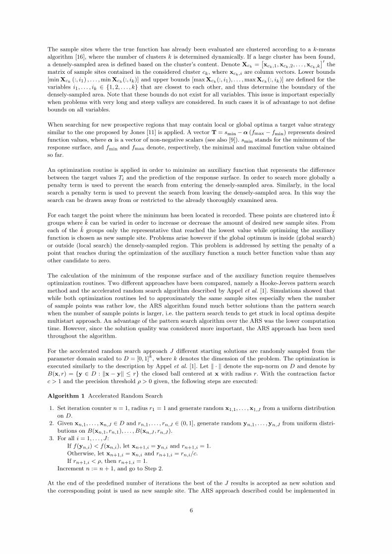
Algorithm 1 Accelerated Random Search

1. Set iteration counter n = 1, radius r1 = 1 and generate random x1,1, . . . ,x1,J from a uniform distribution

on D.

2. Given xn,1, . . . , xn,J ∈ D and rn,1, . . . , rn,J ∈ (0, 1], generate random yn,1, . . . ,yn,J from uniform distri-

butions on B(xn,1, rn,1), . . . , B(xn,J , rn,J ).

3. For all i = 1, . . . , J :

If f(yn,i) < f(xn,i), let xn+1,i = yn,i and rn+1,i = 1.

Otherwise, let xn+1,i = xn,i and rn+1,i = rn,i/c.

If rn+1,i < ρ, then rn+1,i = 1.

Increment n := n + 1, and go to Step 2.

At the end of the predefined number of iterations the best of the J results is accepted as new solution and

the corresponding point is used as new sample site. The ARS approach described could be implemented in

6

parallel so as to execute the calculations for all J starting points simultaneously.

After new sample sites have been determined, the true function is evaluated and new surrogate models are

built. Again cross validation is used to evaluate the goodness of the models and DST is applied to either find

the best single model or the weights of the models in mixtures. The pseudocode of the numerical procedure

is given below.

Algorithm 2 Mixture Surrogate Model Algorithm

1. Find initial set of sample points using for example LHS design, and evaluate costly objective function at

those points.

2. Leave-one-out cross validation: sequentially leave out one sample site and function value at a time and use

remaining data for building different response surfaces (e.g. polynomial regression model, RBF, Kriging,

MARS); use every response surface to re-estimate the function value at the point left out when creating

the models.

3. Calculate goodness values: CC, MAE, RMSE and MAD between true function values and re-estimated

values for each model.

4. (a) If using best single model: use goodness values as evidences and apply Dempster-Shafer theory to

choose the best model.

(b) If using mixture model: use goodness values to calculate weights associated with single models; use

weights for combining models and obtain predictions for every sample site from each mixture model;

calculate CC, RMSE, MAD and MAE for each mixture model, and use the scaled values as evidences;

use Dempster-Shafer-Theory to combine the evidences of the mixture models to choose the best

mixture model.

5. Find the new sample site(s) in one of the following ways:

(a) Local search 1: use the minimum site of the response surface;

(b) Local search 2: define variable domains where already many samples have been taken (i.e. densely-

sampled areas, later on referred to as allowed area) and apply target value strategy that allows search

only from within this region;

(c) Global search: define variable domains where already many samples have been taken (i.e. densely-

sampled areas, later on referred to as forbidden area) and use target value strategy that allows sampling

only outside this region;

6. Evaluate the costly objective function at the new sample site(s).

7. Update response surfaces.

8. Go to step 2.

The algorithm has been implemented in the following three versions:

– Version 1: initially the best mixture surrogate model is used in every iteration; after a predefined number

of failed improvement trials (i.e. new samples that did not improve the current best function value) the

algorithm switches to using only the best single model in every iteration

– Version 2: only the best mixture surrogate model is used in every iteration

– Version 3: only the best single model is used in every iteration.

Initially the algorithm is set to search globally. The criterion described by Holmstrom [9] (later on referred

to as strategy A) has been used to determine whether the surface is fluctuating wildly. If the surface is

fluctuating wildly, the minimum site of the response surface is added as new sample site. Otherwise, forbidden

areas are defined. Target values are calculated and the auxiliary function is minimized taking into account

possible forbidden areas.

The algorithm stays in the global search phase as long as function value improvements can be found. If no

improvements have been obtained, the algorithm switches to the local search phase where the search for the

minimum of the auxiliary function is restricted to the allowed areas. For both search phases it holds that if

no restrictions are given for densely-sampled regions, the minimum of the auxiliary function is sought in the

whole variable domain. Thus, local and global search reach in this case the same results.

On the other hand simulations showed that it might also be useful to include the minimum of the response

surface as new sample site even if the surface is not fluctuating wildly (later on referred to as strategy B).

Therefore, also this approach is examined, and thus three algorithm versions are tested with two different

criteria for adding the minimum site of the response surface.

7

All sample sites must have a sufficient distance to each other, thus avoiding repeated sampling at the same

point. In case no such new sample site can be found, an additional point which maximizes the minimal

distance to all other already sampled points is used as new sample site.

4 Numerical Results

This section summarizes the results of the described algorithms for commonly used global optimization

test problems. All problems have analytical descriptions and the locations of the global optima are known.

All three algorithm versions have been used to solve six different problems. In order to average out the

dependency on the initial experimental design 20 different starting designs have been generated for each

problem and the algorithms were run for every design and every problem.

In the following the name, analytical description, as well as global minima and their locations are given

together with the results of the applied algorithms. The results are presented in tables consisting of

three sections, i.e. one section for every algorithm version. The abbreviations in the first column of each

table reflect the rule for redistributing the global conflict, i.e. D stands for Dempster’s, Y for Yager’s,

I for Inagaki’s, and P for the PCR5 rule. The additional numbers 1, 2 and 3, respectively, indicate the

usage of algorithm version 1, 2 and 3. The columns labeled by min, max and mean denote the minimal,

maximal and average relative error of the algorithms for all 20 test runs. The figures corresponding

to each test problem illustrate the distribution of the relative errors of all 20 runs in the form of box

plots. Also every table and figure consists of parts (a) and (b) which reflect the usage of Holmstroms

criterion (strategy A) for adding the minimum site of the response surface (tables (a)), and the usage of

the second criterion (strategy B) which adds the minimum of the response surface more frequently (tables (b)).

The second and third version of the algorithm were interrupted as soon as 150 function evaluations were

reached. The first version consisted of two phases: at first the model combination was applied until either

the current best solution has a relative error of less than 10%, no improvement has been found within 30

consecutive function evaluations, or the true function has been evaluated more than 150 times. If either of

these conditions has been fulfilled, the algorithm switches to using the best single model in every iteration

until the maximal number of 150 function evaluations has been reached.

In the experiments the following issues were of interest:

1. Did the algorithms find the vicinities of the global minima? If so, did they find all global minima if more

than one was present?

2. Were there significant differences in the results when different conflict redistribution rules were used? If

so, was there one rule that worked best for all problems?

3. How did the choice of the algorithm version influence the results?

4. How good were the results with respect to relative errors?

5. Did the conflict redistribution rule or the choice of the algorithm version influence the computation times

significantly?

6. Which models were chosen and if mixture models were used, which weights were assigned to the con-

tributing models?

4.1 Test Problem B: Branin Function

This is a two variable problem with x1 ∈ [−5, 10] and x2 ∈ [0, 15]. The function is defined by

f(x1, x2) =

„

x2 −5.1x2

1

4π2+

5x1

π− 6

«2

+ 10

„

1 −1

8π

«

cos(x1) + 10.

The function has three global minima with the minimal value f∗ = 0.3979 at the locations

(x∗1, x∗

2) = (−π, 12.275), (x∗1, x∗

2) = (π, 2.275), and (x∗1, x∗

2) = (3π, 2.475). Other local optima do not

exist.

The results of the algorithms for this problem are summarized in Tables 1(a) and 1(b). Every initial

experimental design contained four sample points. For the Branin test function the results show that

8

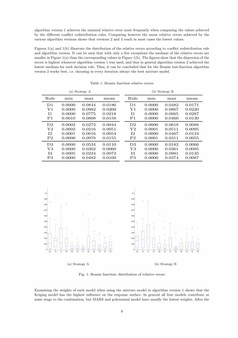
algorithm version 1 achieves the minimal relative error most frequently when comparing the values achieved

by the different conflict redistribution rules. Comparing however the mean relative errors achieved by the

various algorithm versions shows that versions 2 and 3 reach in most cases the lowest values.

Figures 1(a) and 1(b) illustrate the distribution of the relative errors according to conflict redistribution rule

and algorithm version. It can be seen that with only a few exceptions the medians of the relative errors are

smaller in Figure 1(a) than the corresponding values in Figure 1(b). The figures show that the dispersion of the

errors is highest whenever algorithm version 1 was used, and that in general algorithm version 2 achieved the

lowest medians for each decision rule. Thus, it can be concluded that for the Branin test-function algorithm

version 2 works best, i.e. choosing in every iteration always the best mixture model.

Table 1: Branin function relative errors

(a) Strategy A

Rule min max mean

D1 0.0000 0.0844 0.0186Y1 0.0000 0.0982 0.0200I1 0.0000 0.0775 0.0218P1 0.0010 0.0808 0.0158

D2 0.0002 0.0272 0.0044Y2 0.0002 0.0216 0.0051I2 0.0001 0.0616 0.0054P2 0.0000 0.0978 0.0155

D3 0.0000 0.0534 0.0110Y3 0.0000 0.0302 0.0060I3 0.0005 0.0224 0.0073P3 0.0000 0.0482 0.0100

(b) Strategy B

Rule min max mean

D1 0.0000 0.0482 0.0171Y1 0.0000 0.0867 0.0220I1 0.0000 0.0865 0.0287P1 0.0000 0.0460 0.0130

D2 0.0000 0.0618 0.0088Y2 0.0001 0.0511 0.0095I2 0.0000 0.0467 0.0124P2 0.0001 0.0311 0.0055

D3 0.0000 0.0182 0.0066Y3 0.0000 0.0361 0.0095I3 0.0000 0.0981 0.0135P3 0.0000 0.0374 0.0087

0

0.01

0.02

0.03

0.04

0.05

0.06

0.07

0.08

0.09

0.1

D1 Y1 I1 P1 D2 Y2 I2 P2 D3 Y3 I3 P3

(a) Strategy A

0

0.01

0.02

0.03

0.04

0.05

0.06

0.07

0.08

0.09

0.1

D1 Y1 I1 P1 D2 Y2 I2 P2 D3 Y3 I3 P3

(b) Strategy B

Fig. 1: Branin function: distribution of relative errors

Examining the weights of each model when using the mixture model in algorithm version 1 shows that the

Kriging model has the highest influence on the response surface. In general all four models contribute at

some stage to the combination, but MARS and polynomial model have usually the lowest weights. After the

9

switch to using in every iteration only the best single model Kriging proved best in almost all cases. For

algorithm version 2 the results were similar, i.e. the Kriging model obtained the highest weights, while RBF,

polynomial and MARS model contributed the least (polynomial and RBF had in general about the same

weights, while the MARS model had no major impact). When choosing in every iteration only the best single

model, i.e. version 3 of the algorithm, the Kriging model proved best in over 80% of all choices. MARS and

the polynomial model were rarely chosen, and the RBF model was best in about 10% of all cases.

4.2 Test Problem C: Camelback Function

The variables of this bivariate function are constrained to x1 ∈ [−3, 3] and x2 ∈ [−2, 2] and the function is

defined by

f(x1, x2) =

„

4 − 2.1x21 +

x41

3

«

x21 + x1x2 + (−4 + 4x2

2)x22.

The function has global minima at (x∗1, x∗

2) = (−0.0898, 0.7127) and (x∗1, x∗

2) = (0.0898, −0.7127), respec-

tively, where it attains the value f∗ = −1.0316, and other local optima are not present.

The results of the applied algorithms are summarized in Tables 2(a) and 2(b). Initially four sample sites

were used in the experimental designs. The tables show that the minimal relative error is reached when

using algorithm version 1, and either Inagaki’s or Yager’s rule. The tables also show that algorithm version 3

results in the lowest maximal relative error.

The box plots in Figures 2(a) and 2(b) illustrate the dispersion of the relative errors of each algorithm version

and conflict redistribution rule. The plots show that algorithm version 2 results in the highest dispersions

and medians. In general, algorithm version 3, i.e. choosing in every iteration only the best single model as

new response surface, reaches the lowest medians most frequently. Noticeable in Figure 2(b) are the higher

amount and higher values of outliers compared to Figure 2(a).

Table 2: Camelback function relative errors

(a) Strategy A

Rule min max mean

D1 0.0000 0.0298 0.0087Y1 0.0000 0.0506 0.0118I1 0.0000 0.0234 0.0059P1 0.0000 0.0239 0.0072

D2 0.0000 0.1670 0.0317Y2 0.0013 0.1762 0.0510I2 0.0001 0.1437 0.0372P2 0.0000 0.0203 0.0069

D3 0.0003 0.0161 0.0053Y3 0.0000 0.0133 0.0040I3 0.0000 0.0187 0.0062P3 0.0001 0.0136 0.0037

(b) Strategy B

Rule min max mean

D1 0.0000 0.0238 0.0079Y1 0.0000 0.0164 0.0053I1 0.0000 0.0276 0.0097P1 0.0010 0.0411 0.0093

D2 0.0006 0.2684 0.0298Y2 0.0008 0.0937 0.0222I2 0.0006 0.2641 0.0359P2 0.0001 0.0233 0.0055

D3 0.0000 0.0152 0.0040Y3 0.0000 0.0189 0.0038I3 0.0002 0.0274 0.0051P3 0.0001 0.0182 0.0050

The weights of the models contributing to the combined response surface in algorithm version 1 were highest

for Kriging and RBF. The influence of the MARS model was lowest. Similar to the case of the Branin function

the Kriging model is used in most cases after the algorithm switched to using only the best single model. The

RBF model was chosen in a few more cases compared to the Branin function. The weights assigned to the

single models in algorithm version 2 reflect that the Kriging model had in general the highest influence. RBF

and the polynomial model had about the same impact, and the MARS model had again the lowest weights

when contributing to the mixture models. In algorithm version 3 the Kriging model was chosen in most cases.

The polynomial and MARS model had in comparison to other models the worst characteristics and were thus

rarely chosen.

10

0

0.05

0.1

0.15

0.2

0.25

D1 Y1 I1 P1 D2 Y2 I2 P2 D3 Y3 I3 P3

(a) Strategy A

0

0.05

0.1

0.15

0.2

0.25

D1 Y1 I1 P1 D2 Y2 I2 P2 D3 Y3 I3 P3

(b) Strategy B

Fig. 2: Camelback function: distribution of relative errors

4.3 Test Problem G: Goldstein-Price Function

The variable bounds in this problem were x1, x2 ∈ [−2, 2] and the function is defined by

f(x1, x2) =h

1 + (x1 + x2 + 1)2(19 − 14x1 + 3x21 − 14x2 + 6x1x2 + 3x2

2)i

×h

30 + (2x1 − 3x2)2(18 − 31x1 + 12x2

1 + 48x2 − 36x1x2 + 27x22)

i

.

The function has its global minimum at (x∗1, x∗

2) = (0,−1) and attains there the value f∗ = 3. In addition,

the function has several local minima. Since the range of the function values is very large, the logarithm of

the function values has been used during the calculations. The experimental design contained initially four

sample sites.

The data in Tables 3(a) and 3(b) show that the overall lowest minimal relative error of 0.02% was achieved by

each algorithm version. With respect to the minimal maximum and mean relative error algorithm versions 2

and 3 proved most successful. The box plots in Figures 3(a) and 3(b) are rather similar for every decision

rule, but Figure 3(b) contains more outliers. The dispersion of the errors in both figures is about equal. The

results suggest that in general algorithm version 3 should be favored.

The weights assigned to the models contributing to the combination differ from those obtained for the Branin

and the Camelback function. The highest weights in the mixture model of algorithm version 1 were assigned

to the RBF model. The Kriging model had the second highest influence while the MARS and polynomial

model were rather insignificant in most cases. After the switch to using only the best single model RBF was

chosen in over 90% of all cases. Also in algorithm version 2 the RBF model had significantly higher weights

than the other models, and the weights of the Kriging and the polynomial model were in many cases about

equal. Again, the MARS model did not contribute much to the response surface. In algorithm version 3 the

RBF model had the best model characteristics in many cases and was thus most often chosen as best single

model. Polynomial and MARS model had the worst model characteristics.

11

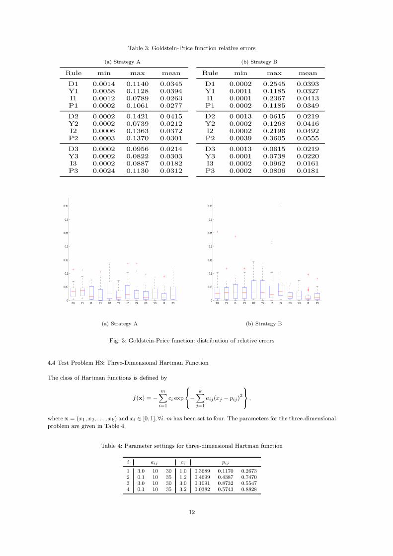
Table 3: Goldstein-Price function relative errors

(a) Strategy A

Rule min max mean

D1 0.0014 0.1140 0.0345Y1 0.0058 0.1128 0.0394I1 0.0012 0.0789 0.0263P1 0.0002 0.1061 0.0277

D2 0.0002 0.1421 0.0415Y2 0.0002 0.0739 0.0212I2 0.0006 0.1363 0.0372P2 0.0003 0.1370 0.0301

D3 0.0002 0.0956 0.0214Y3 0.0002 0.0822 0.0303I3 0.0002 0.0887 0.0182P3 0.0024 0.1130 0.0312

(b) Strategy B

Rule min max mean

D1 0.0002 0.2545 0.0393Y1 0.0011 0.1185 0.0327I1 0.0001 0.2367 0.0413P1 0.0002 0.1185 0.0349

D2 0.0013 0.0615 0.0219Y2 0.0002 0.1268 0.0416I2 0.0002 0.2196 0.0492P2 0.0039 0.3605 0.0555

D3 0.0013 0.0615 0.0219Y3 0.0001 0.0738 0.0220I3 0.0002 0.0962 0.0161P3 0.0002 0.0806 0.0181

0

0.05

0.1

0.15

0.2

0.25

0.3

0.35

D1 Y1 I1 P1 D2 Y2 I2 P2 D3 Y3 I3 P3

(a) Strategy A

0

0.05

0.1

0.15

0.2

0.25

0.3

0.35

D1 Y1 I1 P1 D2 Y2 I2 P2 D3 Y3 I3 P3

(b) Strategy B

Fig. 3: Goldstein-Price function: distribution of relative errors

4.4 Test Problem H3: Three-Dimensional Hartman Function

The class of Hartman functions is defined by

f(x) = −m

X

i=1

ci exp

8

<

:

−k

X

j=1

aij(xj − pij)2

9

=

;

,

where x = (x1, x2, . . . , xk) and xi ∈ [0, 1], ∀i. m has been set to four. The parameters for the three-dimensional

problem are given in Table 4.

Table 4: Parameter settings for three-dimensional Hartman function

i aij ci pij

1 3.0 10 30 1.0 0.3689 0.1170 0.26732 0.1 10 35 1.2 0.4699 0.4387 0.74703 3.0 10 30 3.0 0.1091 0.8732 0.55474 0.1 10 35 3.2 0.0382 0.5743 0.8828

12

This function attains its global optimum f∗ = −3.8628 at the point (x∗1, x∗

2, x∗3) = (0.1146, 0.5556, 0.8525).

The function has four local minima. The results of the three versions of the algorithm are presented in

Tables 5(a) and 5(b). Five points were used as initial experimental design. The data shows that the overall

minimal relative error was achieved when using algorithm version 2. Algorithm versions 2 and 3 give in

general better results than version 1. Noticeable is that the results in Table 5(b) are especially for version 1

and 3 better than the corresponding values in Table 5(a).

The differences between the distributions of the relative errors illustrated in Figures 4(a) and 4(b) are rather

negligible with respect to dispersion and median values. In general Yager’s rule for algorithm version 2 seems

to lead to the best results with respect to median and dispersion of the errors.

Table 5: Three-dimensional Hartman function relative errors

(a) Strategy A

Rule min max mean

D1 0.0002 0.0134 0.0040Y1 0.0006 0.0171 0.0047I1 0.0009 0.0109 0.0040P1 0.0001 0.0093 0.0039

D2 0.0001 0.0070 0.0028Y2 0.0001 0.0091 0.0032I2 0.0002 0.0058 0.0026P2 0.0001 0.0068 0.0025

D3 0.0001 0.0061 0.0028Y3 0.0001 0.0054 0.0028I3 0.0001 0.0116 0.0033P3 0.0001 0.0113 0.0032

(b) Strategy B

Rule min max mean

D1 0.0002 0.0093 0.0034Y1 0.0005 0.0121 0.0043I1 0.0001 0.0106 0.0030P1 0.0005 0.0083 0.0034

D2 0.0001 0.0065 0.0021Y2 0.0009 0.0129 0.0035I2 0.0001 0.0096 0.0025P2 0.0004 0.0069 0.0031

D3 0.0005 0.0062 0.0024Y3 0.0001 0.0054 0.0023I3 0.0006 0.0059 0.0028P3 0.0001 0.0069 0.0027

0

2

4

6

8

10

12

14

16

x 10−3

D1 Y1 I1 P1 D2 Y2 I2 P2 D3 Y3 I3 P3

(a) Strategy A

0

2

4

6

8

10

12

14

16

x 10−3

D1 Y1 I1 P1 D2 Y2 I2 P2 D3 Y3 I3 P3

(b) Strategy B

Fig. 4: Three-dimensional Hartman function: distribution of relative errors

For the three-dimensional Hartman function the Kriging model obtained the highest weights when using

mixture models in algorithm versions 1 and 2. For algorithm version 1 the weights for the MARS model were

higher than for any other already considered test function. The weights of the polynomial model were lowest.

13

On the other hand, in algorithm version 2 the weight of the MARS model was again comparatively low, and

the influence of the Kriging model had increased compared to version 1. When only the best single model

was used, the Kriging model was chosen in over 90% of all cases.

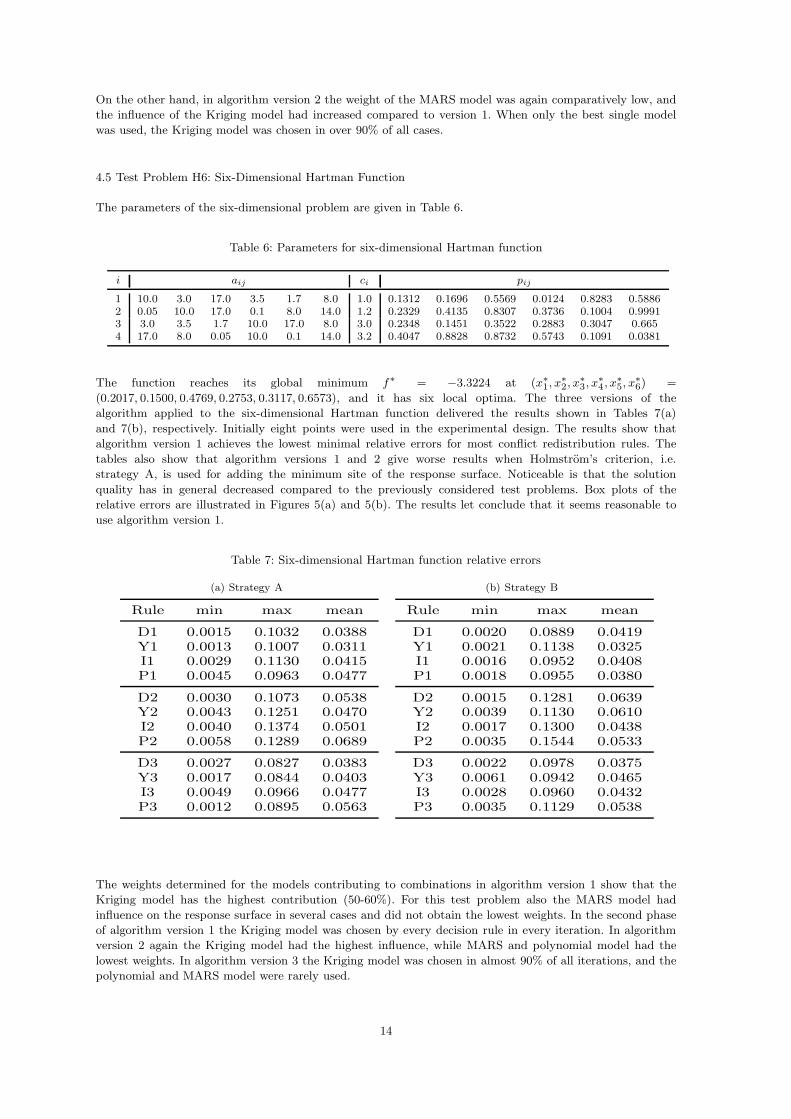
4.5 Test Problem H6: Six-Dimensional Hartman Function

The parameters of the six-dimensional problem are given in Table 6.

Table 6: Parameters for six-dimensional Hartman function

i aij ci pij

1 10.0 3.0 17.0 3.5 1.7 8.0 1.0 0.1312 0.1696 0.5569 0.0124 0.8283 0.58862 0.05 10.0 17.0 0.1 8.0 14.0 1.2 0.2329 0.4135 0.8307 0.3736 0.1004 0.99913 3.0 3.5 1.7 10.0 17.0 8.0 3.0 0.2348 0.1451 0.3522 0.2883 0.3047 0.6654 17.0 8.0 0.05 10.0 0.1 14.0 3.2 0.4047 0.8828 0.8732 0.5743 0.1091 0.0381

The function reaches its global minimum f∗ = −3.3224 at (x∗1, x∗

2, x∗3, x∗

4, x∗5, x∗

6) =

(0.2017, 0.1500, 0.4769, 0.2753, 0.3117, 0.6573), and it has six local optima. The three versions of the

algorithm applied to the six-dimensional Hartman function delivered the results shown in Tables 7(a)

and 7(b), respectively. Initially eight points were used in the experimental design. The results show that

algorithm version 1 achieves the lowest minimal relative errors for most conflict redistribution rules. The

tables also show that algorithm versions 1 and 2 give worse results when Holmstrom’s criterion, i.e.

strategy A, is used for adding the minimum site of the response surface. Noticeable is that the solution

quality has in general decreased compared to the previously considered test problems. Box plots of the

relative errors are illustrated in Figures 5(a) and 5(b). The results let conclude that it seems reasonable to

use algorithm version 1.

Table 7: Six-dimensional Hartman function relative errors

(a) Strategy A

Rule min max mean

D1 0.0015 0.1032 0.0388Y1 0.0013 0.1007 0.0311I1 0.0029 0.1130 0.0415P1 0.0045 0.0963 0.0477

D2 0.0030 0.1073 0.0538Y2 0.0043 0.1251 0.0470I2 0.0040 0.1374 0.0501P2 0.0058 0.1289 0.0689

D3 0.0027 0.0827 0.0383Y3 0.0017 0.0844 0.0403I3 0.0049 0.0966 0.0477P3 0.0012 0.0895 0.0563

(b) Strategy B

Rule min max mean

D1 0.0020 0.0889 0.0419Y1 0.0021 0.1138 0.0325I1 0.0016 0.0952 0.0408P1 0.0018 0.0955 0.0380

D2 0.0015 0.1281 0.0639Y2 0.0039 0.1130 0.0610I2 0.0017 0.1300 0.0438P2 0.0035 0.1544 0.0533

D3 0.0022 0.0978 0.0375Y3 0.0061 0.0942 0.0465I3 0.0028 0.0960 0.0432P3 0.0035 0.1129 0.0538

The weights determined for the models contributing to combinations in algorithm version 1 show that the

Kriging model has the highest contribution (50-60%). For this test problem also the MARS model had

influence on the response surface in several cases and did not obtain the lowest weights. In the second phase

of algorithm version 1 the Kriging model was chosen by every decision rule in every iteration. In algorithm

version 2 again the Kriging model had the highest influence, while MARS and polynomial model had the

lowest weights. In algorithm version 3 the Kriging model was chosen in almost 90% of all iterations, and the

polynomial and MARS model were rarely used.

14

0

0.02

0.04

0.06

0.08

0.1

0.12

0.14

0.16

D1 Y1 I1 P1 D2 Y2 I2 P2 D3 Y3 I3 P3

(a) Strategy A

0

0.02

0.04

0.06

0.08

0.1

0.12

0.14

0.16

D1 Y1 I1 P1 D2 Y2 I2 P2 D3 Y3 I3 P3

(b) Strategy B

Fig. 5: Six-dimensional Hartman function: distribution of relative errors

4.6 Test Problem S: Shekel Function

The general definition of this function type is

f(x) =m

X

i=1

1

ci +Pk

j=1(xj − aji)2,

and the variables are bounded to x ∈ [0, 10]. The parameters are

A =

2

6

6

4

4 1 8 6 3 2 5 8 6 7

4 1 8 6 7 9 5 1 2 3.6

4 1 8 6 3 2 3 8 6 7

4 1 8 6 7 9 3 1 2 3.6

3

7

7

5

, and c =1

10[1, 2, 2, 4, 4, 6, 3, 7, 5, 5]′ .

The Shekel functions have a very steep global minimum at xi = 4,∀i. In the four-dimensional case the op-

timal function value is f∗ = −10.5364, and the number of local optima is m, which is in the considered case 10.

The initial experimental design contained 16 points. All versions of the algorithm had trouble finding the

global optimum (see Tables 8(a) and 8(b)). The overall best results were achieved by algorithm version 1

in both tables. The results in Table 8(b) are in several cases better than the corresponding entries in Table 8(a).

Figures 6(a) and 6(b) show the distribution of the relative errors for each algorithm version and conflict

redistribution rule. Compared to all other previously considered test problems, the results are much worse.

The box plots in Figure 6(b) have more outliers than those in Figure 6(a), but otherwise there are no

significant differences between strategies A and B.

Also for this test function the weights assigned to the Kriging model were highest in algorithm version 1.

The MARS model obtained the lowest weights. However, the difference between the weights for Kriging,

polynomial and RBF model was much smaller than for the previously considered test problems. After

the switch to using only the best single model Kriging was chosen in most cases, but also RBF had in

several cases the best model characteristics. The polynomial and MARS model have never obtained a better

evaluation than Kriging or RBF. The same statements hold for algorithm versions 2 and 3. The weights of

the models in version 2 were on average as for the first stage of algorithm version 1. In version 3 Kriging and

RBF were chosen as best models most often.

15

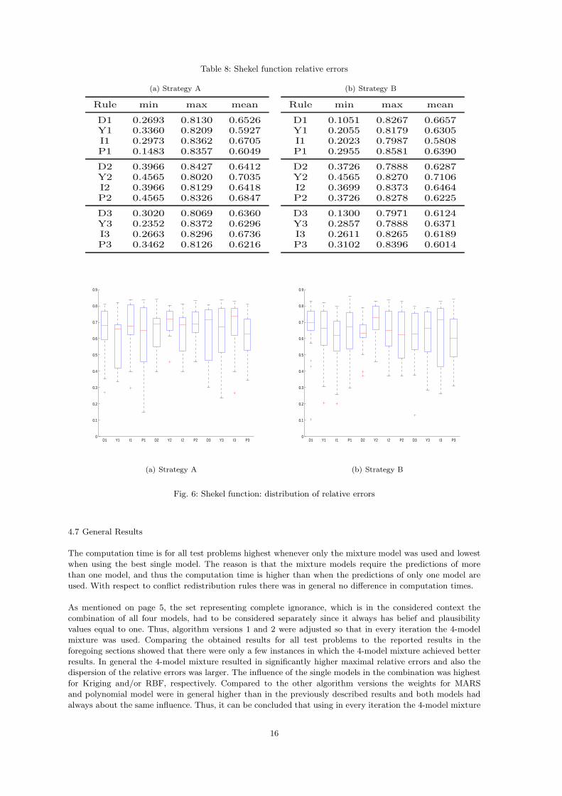
Table 8: Shekel function relative errors

(a) Strategy A

Rule min max mean

D1 0.2693 0.8130 0.6526Y1 0.3360 0.8209 0.5927I1 0.2973 0.8362 0.6705P1 0.1483 0.8357 0.6049

D2 0.3966 0.8427 0.6412Y2 0.4565 0.8020 0.7035I2 0.3966 0.8129 0.6418P2 0.4565 0.8326 0.6847

D3 0.3020 0.8069 0.6360Y3 0.2352 0.8372 0.6296I3 0.2663 0.8296 0.6736P3 0.3462 0.8126 0.6216

(b) Strategy B

Rule min max mean

D1 0.1051 0.8267 0.6657Y1 0.2055 0.8179 0.6305I1 0.2023 0.7987 0.5808P1 0.2955 0.8581 0.6390

D2 0.3726 0.7888 0.6287Y2 0.4565 0.8270 0.7106I2 0.3699 0.8373 0.6464P2 0.3726 0.8278 0.6225

D3 0.1300 0.7971 0.6124Y3 0.2857 0.7888 0.6371I3 0.2611 0.8265 0.6189P3 0.3102 0.8396 0.6014

0

0.1

0.2

0.3

0.4

0.5

0.6

0.7

0.8

0.9

D1 Y1 I1 P1 D2 Y2 I2 P2 D3 Y3 I3 P3

(a) Strategy A

0

0.1

0.2

0.3

0.4

0.5

0.6

0.7

0.8

0.9

D1 Y1 I1 P1 D2 Y2 I2 P2 D3 Y3 I3 P3

(b) Strategy B

Fig. 6: Shekel function: distribution of relative errors

4.7 General Results

The computation time is for all test problems highest whenever only the mixture model was used and lowest

when using the best single model. The reason is that the mixture models require the predictions of more

than one model, and thus the computation time is higher than when the predictions of only one model are

used. With respect to conflict redistribution rules there was in general no difference in computation times.

As mentioned on page 5, the set representing complete ignorance, which is in the considered context the

combination of all four models, had to be considered separately since it always has belief and plausibility

values equal to one. Thus, algorithm versions 1 and 2 were adjusted so that in every iteration the 4-model

mixture was used. Comparing the obtained results for all test problems to the reported results in the

foregoing sections showed that there were only a few instances in which the 4-model mixture achieved better

results. In general the 4-model mixture resulted in significantly higher maximal relative errors and also the

dispersion of the relative errors was larger. The influence of the single models in the combination was highest

for Kriging and/or RBF, respectively. Compared to the other algorithm versions the weights for MARS

and polynomial model were in general higher than in the previously described results and both models had

always about the same influence. Thus, it can be concluded that using in every iteration the 4-model mixture

16

does not lead to improved results.

In addition to investigating how close the algorithms get to the global optima with respect to relative errors,

it is of interest if and how many global optima could be detected. Tables 9(a) and 9(b) show the fractions

each algorithm was able to sample in the vicinity of the global minima. The vicinity was here defined in

terms of the distance of the sample sites to the known locations of global and local optima. The tables

show that for the Goldstein-Price and the three-dimensional Hartman function, all algorithm versions found

the vicinity of the corresponding global minima without getting trapped in local optima. As the results

show, algorithm version 3 found the highest number of global minima for all decision rules when the prob-

lem dimension is at most three. However, for higher dimensions algorithm versions 2 and 1 are more successful.

In general the PCR5 rule proved the most successful with respect to the number of global minima found.

Compared to the quality of the results however, the PCR5 rule was not always the best, i.e. PCR5

did not always lead to the lowest errors. Interesting are the results for the Shekel function. The lowest

relative error obtained was 10.51% by Dempster’s conflict redistribution rule and using algorithm version 1.

However, all algorithms found the vicinity of the global minima in 50-95% of all test cases, but still the

relative errors are not very satisfying. Thus, it can be concluded that the algorithms failed in searching

thoroughly locally, and thus they missed the very steep optimum of this function. Therefore, the local search

strategy of the algorithms must be enhanced so that also the relative errors for such functions can be decreased.

Comparing the entries of Tables 9(a) and 9(b) shows that the number of global minima found was higher

when using Holmstrom’s criterion for adding the minimum site of the response surface. Based on these and

the foregoing results (i.e. tables and figures corresponding to strategy A) it seems reasonable to employ

Holmstrom’s criterion. On the other hand, since the algorithm versions 1 and 2 proved more successful with

increasing dimensions, they should also be used for problems containing more than six variables.

Table 9: Number of basins of global optima found (in %)

(a) Strategy A

Rule B C G H3 S H6

D1 91.67 95.00 100.00 100.00 65.00 85.00Y1 76.67 100.00 100.00 100.00 75.00 95.00I1 86.67 100.00 100.00 100.00 50.00 80.00P1 83.33 100.00 100.00 100.00 70.00 80.00

D2 86.67 65.00 100.00 100.00 85.00 80.00Y2 83.33 57.50 100.00 100.00 60.00 90.00I2 81.67 72.50 100.00 100.00 75.00 90.00P2 81.67 100.00 100.00 100.00 75.00 85.00

D3 96.67 100.00 100.00 100.00 60.00 80.00Y3 96.67 100.00 100.00 100.00 60.00 80.00I3 95.00 100.00 100.00 100.00 50.00 85.00P3 100.00 100.00 100.00 100.00 65.00 70.00

(b) Strategy B

Rule B C G H3 S H6

D1 85.00 100.00 100.00 100.00 55.00 75.00Y1 81.67 97.50 100.00 100.00 65.00 85.00I1 85.00 95.00 100.00 100.00 75.00 85.00P1 83.33 100.00 100.00 100.00 65.00 80.00

D2 81.67 77.50 100.00 100.00 80.00 90.00Y2 81.67 80.00 100.00 100.00 45.00 85.00I2 25.00 82.50 100.00 100.00 70.00 85.00P2 81.67 100.00 100.00 100.00 60.00 85.00

D3 96.67 100.00 100.00 100.00 60.00 80.00Y3 96.67 100.00 100.00 100.00 50.00 85.00I3 95.00 100.00 100.00 100.00 45.00 80.00P3 100.00 100.00 100.00 100.00 65.00 65.00

Tables 10(a) and 10(b) show the minimum number of true function evaluations that were necessary to reach

relative errors of less than 1% in all 20 runs (note that the Shekel test function is not included since relative

errors of less than 1% were not achieved). The numbers show that Inagaki’s as well as the PCR5 rule are

most successful when using algorithm version 1. For algorithm version 2 Yager’s rule proved most often

successful, and Dempster’s rule worked best when algorithm version 3 was used. Comparing the overall

performance of all conflict redistribution rules shows that Inagaki’s rule is the most promising.

Tables 11(a) and 11(b) show the number of simulations in which relative errors of less than 1% have been

reached, i.e. in how many of the 20 simulation runs of each method for every problem the global optimum could

be approximated with an error of less than 1%. For example, with Strategy A the method D1 found for the

test problem B in 10 out of 20 simulation runs the global optimum with an error of less than 1%. For algorithm

version 1 again Inagaki’s rule is most successful, while Dempster’s or Yager’s rule are recommendable when

17

Table 10: Minimum number of function evaluations to reach less than 1% relative error

(a) Strategy A

Rule B C G H3 H6

D1 26 15 47 30 72Y1 23 22 52 19 56I1 12 22 39 20 40P1 27 10 33 16 67

D2 23 16 46 21 70Y2 12 15 42 14 60I2 25 14 50 18 63P2 27 9 65 21 58

D3 12 17 29 17 62Y3 27 25 46 22 96I3 21 9 29 21 129P3 14 21 42 20 102

(b) Strategy B

Rule B C G H3 H6

D1 33 24 22 22 79Y1 17 10 54 18 101I1 14 22 19 13 37P1 25 24 29 17 66

D2 17 24 49 24 79Y2 12 15 40 19 51I2 27 8 69 20 71P2 17 11 48 20 88

D3 12 15 30 19 51Y3 25 16 29 28 62I3 13 22 36 20 89P3 15 23 22 22 64

using algorithm version 2. For algorithm version 3 Dempster’s rule works best. An overall comparison of the

results of all conflict redistribution rules shows that Yager’s and the PCR5 rule have the best performance.

Thus, together with the results from Tables 10 it seems promising to use Inagaki’s rule when algorithm

version 1 is used, Yager’s rule in algorithm version 2, and Dempster’s rule with algorithm version 3 in order

to obtain the best results.

Table 11: Number of simulations in which less than 1% relative error found

(a) Strategy A

Rule B C G H3 H6

D1 10 14 4 19 7Y1 17 8 5 20 3I1 13 15 10 20 5P1 6 13 3 18 10

D2 16 5 10 20 6Y2 16 18 6 20 5I2 9 15 9 19 6P2 19 7 8 20 5

D3 13 16 11 19 3Y3 9 13 10 20 2I3 13 15 7 20 1P3 13 18 7 19 2

(b) Strategy B

Rule B C G H3 H6

D1 7 11 8 20 7Y1 14 10 7 20 2I1 15 18 6 20 6P1 9 16 6 18 9

D2 16 7 7 19 2Y2 11 16 7 20 2I2 7 12 4 18 5P2 12 7 6 20 4

D3 14 18 13 20 2Y3 11 13 6 20 5I3 17 16 4 20 2P3 13 16 10 20 4

5 Conclusions and Future Research Topics

This paper has presented the application of Dempster-Shafer theory to surrogate model choice and surrogate

model combination in global optimization problems. Model characteristics obtained from cross validation

reflect good and bad properties of the considered models and their combinations, respectively. Different

rules for redistributing the conflict originating from good and bad properties of the same model have been

considered and compared. The advantage of this approach is that no parameters need to be adjusted in

18

order to emphasize or restrict the influence of conflicting model characteristics. Also the impact of the usage

of mixture models, single models and a combination of both have been examined and results compared on

global optimization test problems.

The results showed that the proposed approach proved successful in finding the global minima of most test

problems. The exploration of the variable domain had a good ratio of local and global search, and thus the

vicinities of global minima were detected and the actual global minimum could, with the exception of one

test function, be found with average relative errors of less than 1%. The algorithms had trouble only with

the test function which had a very steep global minimum. Although the vicinity of the global minimum has

been detected and several samples have been taken in the prospective region, the algorithm failed to search

thoroughly enough in order to find the actual location of the minimum. This implies that the used local

search procedure should still be improved in order to detect also very steep minima. In connection with this

issue is also the adjustment of parameters determining for example when to invoke the local search, how

many new sample sites should be taken, or the definition of the search area when optimizing the auxiliary

function.

The results also indicated that the success of the algorithms in finding all global minima was to some extent

dependent on the used conflict redistribution rule and the algorithm version. In general, the proportional

conflict redistribution rule led to the best variable domain exploration. On the other hand, this rule did

not always lead to the lowest relative errors, and thus the possibility of linking the conflict redistribution

rule to the search phase (local or global) should be examined in further experiments. With respect to

variable domain exploration and relative errors the results showed that with increasing problem dimension

the algorithms applying model combinations become more favorable. However, this issue should further be

examined in real-world application problems. The amount and type of model characteristics used for the

evaluation of the goodness of the single surrogate models should then also be derived from the specific

application, i.e. in some cases certain model characteristics may be more important than others and should

thus be emphasized in the model evaluation. In connection with real-world applications is also the extension

of the algorithms to handling linear and nonlinear constraints as well as integer conditions which can be

assumed to be present in most engineering problems. Further testing of the implemented procedures on

higher dimensional problems and an analysis of their efficiency is necessary. The testing showed that there

are in general no major differences in computation times when using different conflict redistribution rules.

Differences arise only when using single or mixture models as response surfaces. In general it can be assumed

that evaluating the true function is much more costly than building the surrogate models, and thus the

described approach is feasible also with respect to computation times.

With respect to the computational demand the described algorithms are suitable for distributed computing.

For example the cross validation of the single models is an ”embarrassingly parallel” computation, as is

the procedure for minimizing the auxiliary functions and the response surface. In case the cross validation

becomes computationally too expensive, it is possible to consider the re-evaluation and choice of the best

model only every, say, lth iteration, or to switch to a k-fold cross validation strategy after a certain number

of samples has been obtained. An important issue connected with the first possibility is the determination of

l, i.e. how often the (mixture) model should be re-adjusted while keeping the solution quality at a high level.

These extensions of the algorithms will be considered in future developments.

Acknowledgements

We would like to thank the anonymous reviewers for their helpful comments.

References

1. M. J. Appel, R. Labarre, and D. Radulovic. On accelerated random search. SIAM Journal on Optimiza-

tion, 14708-731, 2003.

2. M. Bjorkman and K. Holmstrom. Global optimization of costly nonconvex functions using radial basis

functions. Optimization and Engineering, 1:373–397, 2001.

3. C. Currin, T. Mitchell, M. Morris, and D. Ylvisaker. A bayesian approach to the design and analysis of

computer experiments. Technical report, Oak Ridge National Laboratory, Oak Ridge, TN, 1988.

4. A. P. Dempster. A generalization of bayesian inference. Journal of the Royal Statistical Society, Series B

30:205–247, 1968.

19

5. J. Duchon. Constructive Theory of Functions of Several Variables. Springer-Verlag, Berlin, 1977.

6. J. H. Friedman. Multivariate adaptive regresion splines. The Annals of Statistics, 19:1–141, 1991.

7. B. Glaz, P.P. Friedmann, and L. Liu. Surrogate based optimization of helicopter rotor blades for vibration

reduction in forward flight. Structural and Multidisciplinary Optimization, 35:341–363, 2008.

8. T. Goel, R. T. Haftka, W. Shyy, and N. V. Queipo. Ensemble of surrogates. Structural Multidisciplinary

Optimization, 33:199–216, 2007.

9. K. Holmstrom. An adaptive radial basis algorithm (ARBF) for expensive black-box global optimization.

Journal of Global Optimization, 41:447–464, 2008.

10. T. Inagaki. Interdependence between safety-control policy and multiple-sensor schemes via Dempster-

Shafer theory. IEEE Transactions on Reliability, 40:182–188, 1991.

11. D. R. Jones. A taxonomy of global optimization methods based on response surfaces. Journal of Global

Optimization, 21:345–383, 2001.

12. D. R. Jones, M. Schonlau, and W. J. Welch. Efficient global optimization of expensive black-box functions.

Journal of Global Optimization, 13:455–492, 1998.

13. X. B. Lam, Y. S. Kim, A. D. Hoang, and C. W. Park. Coupled aerostructural design optimization using

the kriging model and integrated multiobjective optimization algorithm. Journal of Optimization Theory

and Applications, DOI: 10.1007/s10957-009-9520-9, 2009.

14. X. Liao, Q. Li, X. Yang, W. Zhang, and W. Li. Multiobjective optimization for crash safety design

of vehicles using stepwise regression model. Structural and Multidisciplinary Optimization, 35:561–569,

2008.

15. S. N. Lopheven, H. B. Nielsen, and J. Søndergaard. DACE a matlab kriging toolbox. Technical report,

Technical Report IMM-TR-2002-12, 2002.

16. J.B. MacQueen. Some methods for classification and analysis of multivariate observations. Proceedings of

the Fifth Berkeley Symposium on Mathematical Statistics and Probability, University of California Press,

1:281–297, 1967.

17. J. D. Martin and T. W. Simpson. Use of kriging models to approximate deterministic computer models.

AIAA Journal, 43:853–863, 2005.

18. G. Matheron. Principles of geostatistics. Economic Geology, 58:1246–1266, 1963.

19. R. C. Morgans, A. C. Zander, C. H. Hansen, and D. J. Murphy. EGO shape optimization of horn-loaded

loudspeakers. Optimization and Engineering, 9:361–374, 2008.

20. R. H. Myers and D. C. Montgomery. Response Surface Methodology, Process and Product Optimization

using Designed Experiments. Wiley-Interscience Publication, 1995.

21. M. J. D. Powell. The Theory of Radial Basis Function Approximation in 1990. Advances in Numerical

Analysis, vol. 2: wavelets, subdivision algorithms and radial basis functions. Oxford University Press,

Oxford, pp. 105-210, 1992.

22. M. J. D. Powell. Recent Research at Cambridge on Radial Basis Functions. New Developments in

Approximation Theory, pp. 215-232. Birkhauser, Basel, 1999.

23. N. V. Queipo, R. T. Haftka, W. Shyy, T. Goel, R. Vaidyanathan, and P. K. Tucker. Surrogate-based

analysis and optimization. Progress in Aerospace Sciences, 41:1–28, 2005.

24. R. G. Regis and C. A. Shoemaker. Constrained global optimization of expensive black box functions

using radial basis functions. Journal of Global Optimization, 31:153–171, 2005.

25. R. G. Regis and C. A Shoemaker. Improved strategies for radial basis function methods for global

optimization. Journal of Global Optimization, 37:113–135, 2007.

26. G. Shafer. A Mathematical Theory of Evidence. Princeton University Press, 1976.

27. F. Smarandache and J. Dezert. Information fusion based on new proportional conflict redistribution rules.

In 7th International Conference on Information Fusion, pp. 907-914, 2005.

28. F. A. C. Viana and R. T. Haftka. Using multiple surrogates for minimization of the RMS error in

metamodeling. In Proceedings of the ASME 2008 International Design Engineering Technical Conferences

& Computers and Information in Engineering Conference DETC2008-49240, 2008.

29. R. R. Yager. On the Dempster-Shafer framework and new combination rules. Information Sciences,

41:93–137, 1987.

30. R. J. Yang, N. Wang, C. H. Tho, J. P. Bobineau, and B.P. Wang. Metamodeling development for vehicle

frontal impact simulation. Journal of Mechanical Design, 127:1014–1021, 2005.

31. L. A. Zadeh. Review of book: A mathematical theory of evidence. The AI Magazine, 5:81–83, 1984.

32. P. Zhu, Y. Zhang, and G.-L. Chen. Metamodel-based lightweight design of an automotive front-body

structure using robust optimization. Proceedings of the Institution of Mechanical Engineers, Part D:

Journal of Automobile Engineering, DOI: 10.1243/09544070JAUTO1045, 2009.

20