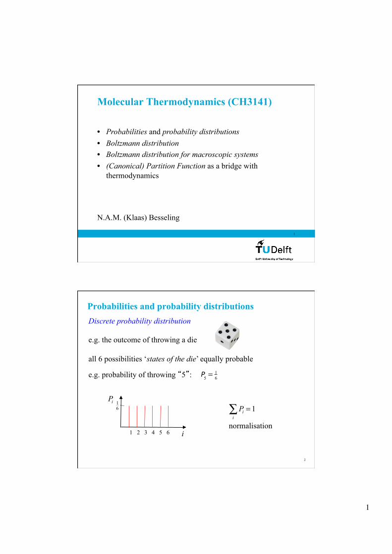
1

1

Molecular Thermodynamics (CH3141)

N.A.M. (Klaas) Besseling

•  Probabilities and probability distributions •  Boltzmann distribution •  Boltzmann distribution for macroscopic systems •  (Canonical) Partition Function as a bridge with

thermodynamics

Probabilities and probability distributions Discrete probability distribution e.g. the outcome of throwing a die all 6 possibilities ‘states of the die’ equally probable

e.g. probability of throwing “5”:

P5 =16

�

Pi

�

16

i

2

�

Pii∑ = 1

normalisation 1 2 3 4 5 6

2

3

‘Subsets of outcomes’

PI = Pii∈I∑

The probability of any outcome belonging to a specific subset is the sum of the probabilities of the outcomes belonging to that subset

example with a die

the chance of an odd number: (the odd numbers are a subset of all numbers)

Podd = P1 +P3 +P5 =16+ 16+ 16= 36

Podd = Piodd#i∑

i∈I∑ denotes the sum over all i

that belong to subset I

In Molecular Thermodynamics we will often deal with

‘mathematically’

4

Euro crisis A pile of euro coins The number of coins from country c and year j is indicated as The probability to draw a coin from country c and year j is

nc , j

Pc , j =nc , jnc , jc , j∑

=nc , jN

where is the total number of coins N = nc , jc , j∑Write an expression for the probability to draw a coin from country c Write an expression for the probability to draw a coin from year j

Pc = Pc , jj∑ =

nc , jj∑N

Pj = Pc , jc∑ =

nc , jc∑N

?

‘Subsets of outcomes’

3

5

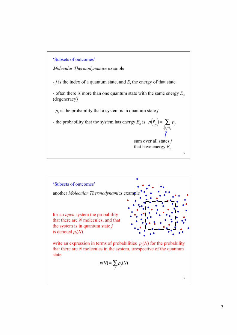
‘Subsets of outcomes’

Molecular Thermodynamics example

- j is the index of a quantum state, and Ej the energy of that state - often there is more than one quantum state with the same energy Ea (degeneracy) - pj is the probability that a system is in quantum state j - the probability that the system has energy Ea is p Ea( ) = pj

j E j=Ea

∑

sum over all states j that have energy Ea

6

‘Subsets of outcomes’

another Molecular Thermodynamics example

for an open system the probability that there are N molecules, and that the system is in quantum state j is denoted pj(N) write an expression in terms of probabilities pj(N) for the probability that there are N molecules in the system, irrespective of the quantum state

p(N)= pjj∑ (N)

?

4

7

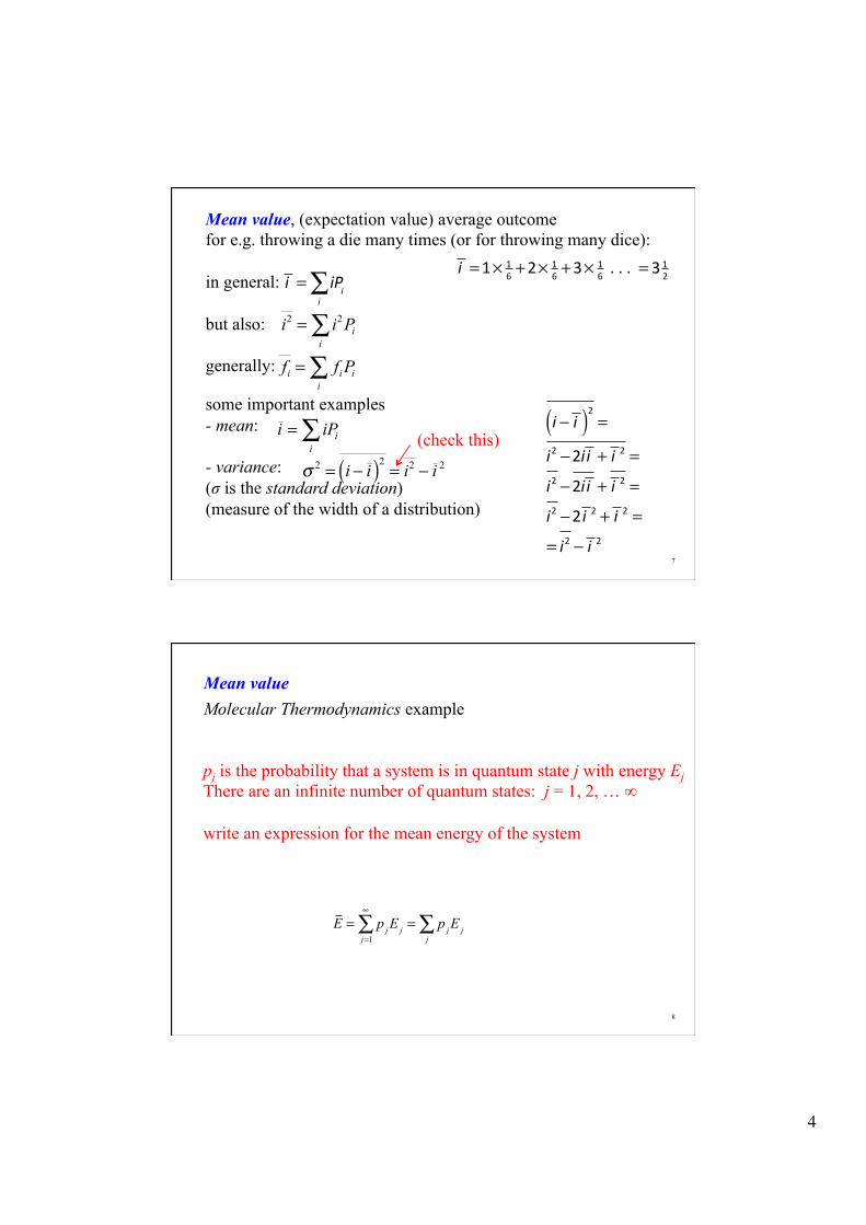
Mean value, (expectation value) average outcome for e.g. throwing a die many times (or for throwing many dice): in general: but also: generally: some important examples - mean: - variance: (σ is the standard deviation) (measure of the width of a distribution)

�

i = iPii∑

�

i2 = i2Pii∑

�

fi = fi Pii∑

i =1× 16 +2×

16 +3×

16 %.%.%.% = 3

12

�

σ 2 = i − i ( )2= i2 − i 2

(check this) i − i( )2 =i2 −2i i + i 2 =

i2 −2i i + i 2 =

i2 −2 i 2 + i 2 =

= i2 − i 2

?

i = iPii∑

8

Molecular Thermodynamics example Mean value

pj is the probability that a system is in quantum state j with energy Ej There are an infinite number of quantum states: j = 1, 2, … ∞ write an expression for the mean energy of the system

E = p jE jj=1

∞

∑ = p jE jj∑

?

5

9

E.g. throw a die twice what is the probability that first throw yields “5”, second throw yields “2”:

(product of independent chances) if order does not matter:

P5,2 = P5P2 = 1616

P5P2 + P2P5 = 2P2P5 = 2 16 16

Combination of independent events

nr. of permutations nr. of ways to get “2” and “5”

- such “nrs. of ways” are very important in Molecular Thermodynamics - molecular basis of Entropy

10

the 6 permutations of three distinguishable balls

this number of permutations is calculated as 3x2x1 = 3!

- for the 1st position 3 possible colors - for the 2nd position 2 possible colors - for the 3rd position 1 possible colors

or, equivalently

- for the 1st color 3 possible positions - for the 2nd colors 2 possible positions - for the 3rd colors 1 possible position

6

11

Flip 6 coins, and lay them out; e.g.

what would the number of permutations be if we would have 6 different objects rather than just two (head and tail)? what is the number of permutations for 2 heads and 4 tails?

6! ?

need to devide by 2! and by 4!

. . . .

what is the number of permutations for 2 heads and 4 tails?

→ 6!2!4!

?

or

12

Continuous distributions

x x+dx

�

P(x)dx

�

P(x)dx−∞

∞

∫ = 1normalisation: is dimensionless (when x has dimension [x], then P(x) has dimension 1/[x]) mean f :

(f is some function of random variable x): e.g.

�

f (x) = f (x)P(x)dx−∞

∞

∫

�

x = xP(x)dx−∞

∞

∫

�

x2 = x2P(x)dx−∞

∞

∫

�

↑P

�

x →

x is a continuous random variable

-  One cannot say “P is the probability of x”!

- is the probability of a value between x and x+dx .

�

P(x)dx

�

P(x)dx

7

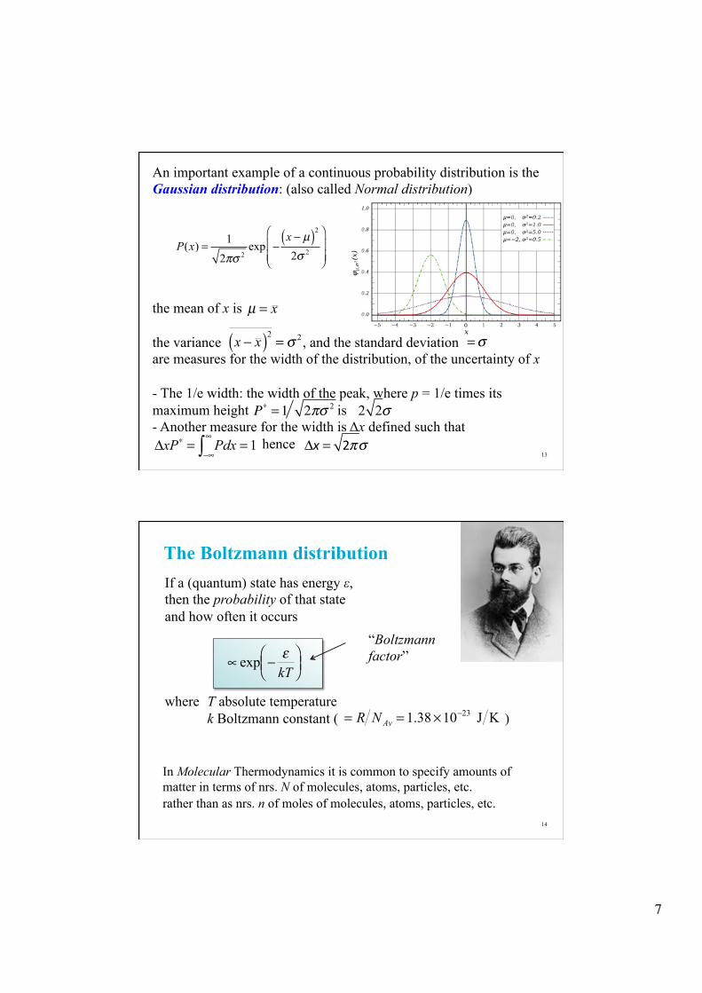
An important example of a continuous probability distribution is the Gaussian distribution: (also called Normal distribution) the mean of x is the variance , and the standard deviation are measures for the width of the distribution, of the uncertainty of x - The 1/e width: the width of the peak, where p = 1/e times its maximum height is - Another measure for the width is Δx defined such that hence

13

P(x) = 1

2πσ 2exp −

x − µ( )22σ 2

⎛

⎝⎜⎜

⎞

⎠⎟⎟

�

µ = x

�

x − x ( )2= σ 2

2 2σP∗ =1 2πσ 2

�

ΔxP∗ = Pdx−∞

∞

∫ = 1 Δx = 2πσ

=σ

If a (quantum) state has energy ε, then the probability of that state and how often it occurs where T absolute temperature

k Boltzmann constant ( )

14

The Boltzmann distribution

�

∝ exp − εkT

⎛ ⎝ ⎜

⎞ ⎠ ⎟

�

= R N Av = 1.38×10−23 J K

In Molecular Thermodynamics it is common to specify amounts of matter in terms of nrs. N of molecules, atoms, particles, etc. rather than as nrs. n of moles of molecules, atoms, particles, etc.

“Boltzmann factor”

8

15

high T

ε

1

�

exp − εkT

⎛ ⎝ ⎜

⎞ ⎠ ⎟

low T

�

e−1

kT kT

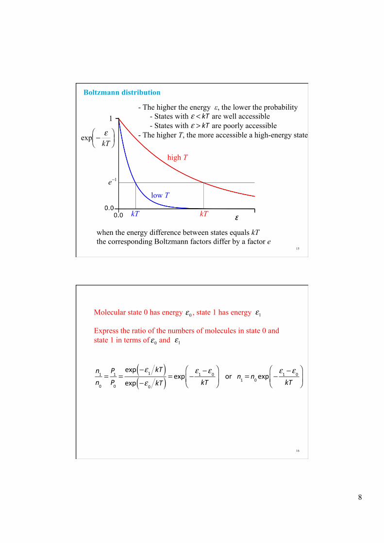
Boltzmann distribution

- The higher the energy ε, the lower the probability - States with are well accessible - States with are poorly accessible

- The higher T, the more accessible a high-energy state

ε < kTε > kT

when the energy difference between states equals kT the corresponding Boltzmann factors differ by a factor e

n1n0

=P1P0

=exp −ε1 kT( )exp −ε0 kT( ) = exp −

ε1 −ε0

kT

⎛

⎝⎜⎞

⎠⎟&&&or&&&n1 = n0 exp −

ε1 −ε0

kT

⎛

⎝⎜⎞

⎠⎟

16

Molecular state 0 has energy , state 1 has energy Express the ratio of the numbers of molecules in state 0 and state 1 in terms of and

�

ε1

�

ε0

�

ε1

�

ε0

?

9

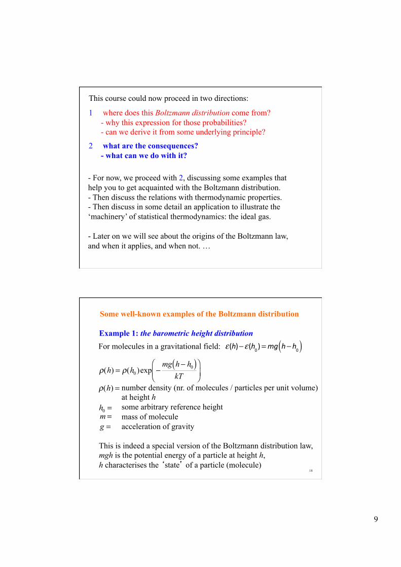
This course could now proceed in two directions:

1  where does this Boltzmann distribution come from? - why this expression for those probabilities? - can we derive it from some underlying principle?

2  what are the consequences? - what can we do with it?

- For now, we proceed with 2, discussing some examples that help you to get acquainted with the Boltzmann distribution. - Then discuss the relations with thermodynamic properties. - Then discuss in some detail an application to illustrate the ‘machinery’ of statistical thermodynamics: the ideal gas. - Later on we will see about the origins of the Boltzmann law, and when it applies, and when not. …

18

Example 1: the barometric height distribution

�

ρ(h) = ρ(h0 )exp −mg h − h0( )

kT⎛

⎝ ⎜ ⎞

⎠ ⎟

�

ρ(h) = number density (nr. of molecules / particles per unit volume) at height h some arbitrary reference height mass of molecule acceleration of gravity

�

h0 =

For molecules in a gravitational field:

�

m =

�

g =

This is indeed a special version of the Boltzmann distribution law, mgh is the potential energy of a particle at height h, h characterises the ‘state’ of a particle (molecule)

ε(h)−ε(h0)=mg h−h0( )

Some well-known examples of the Boltzmann distribution

10

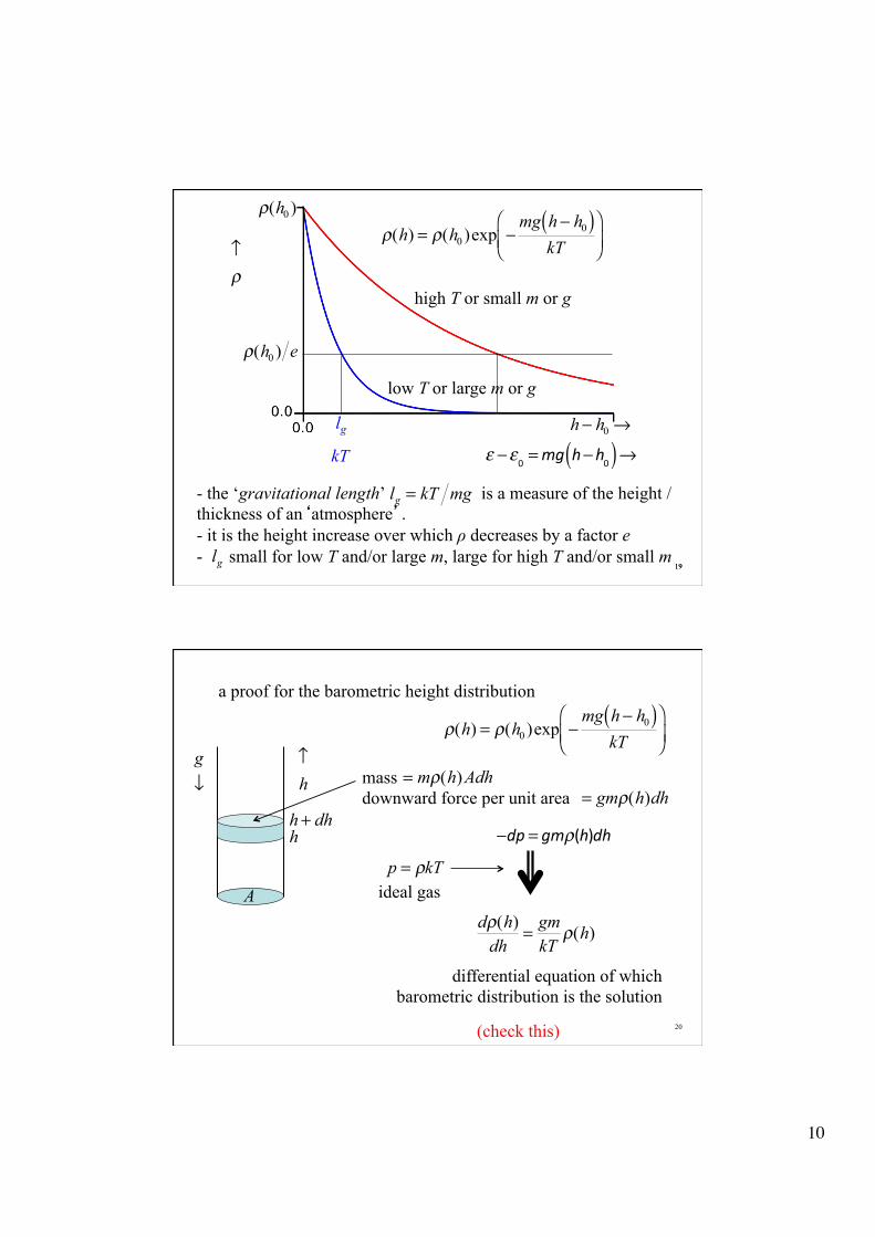
19 19

high T or small m or g

1

low T or large m or g

�

ρ(h0 ) e

�

ρ(h0 )

- the ‘gravitational length’ is a measure of the height / thickness of an‘atmosphere’. - it is the height increase over which ρ decreases by a factor e - small for low T and/or large m, large for high T and/or small m

�

lg = kT mg

�

lg

�

h − h0 →

�

↑ρ

lg

ε −ε0 =mg h−h0( )→

�

ρ(h) = ρ(h0 )exp −mg h − h0( )

kT⎛

⎝ ⎜ ⎞

⎠ ⎟

kT

20

a proof for the barometric height distribution

�

h + dh

�

h

�

↑h

�

g↓

A

mass downward force per unit area

�

= mρ(h)Adh

�

= gmρ(h)dh

�

dρ(h)dh

= gmkT

ρ(h)

�

p = ρkTideal gas

differential equation of which barometric distribution is the solution

(check this)

�

ρ(h) = ρ(h0 )exp −mg h − h0( )

kT⎛

⎝ ⎜ ⎞

⎠ ⎟

−dp = gmρ(h)dh

11

21

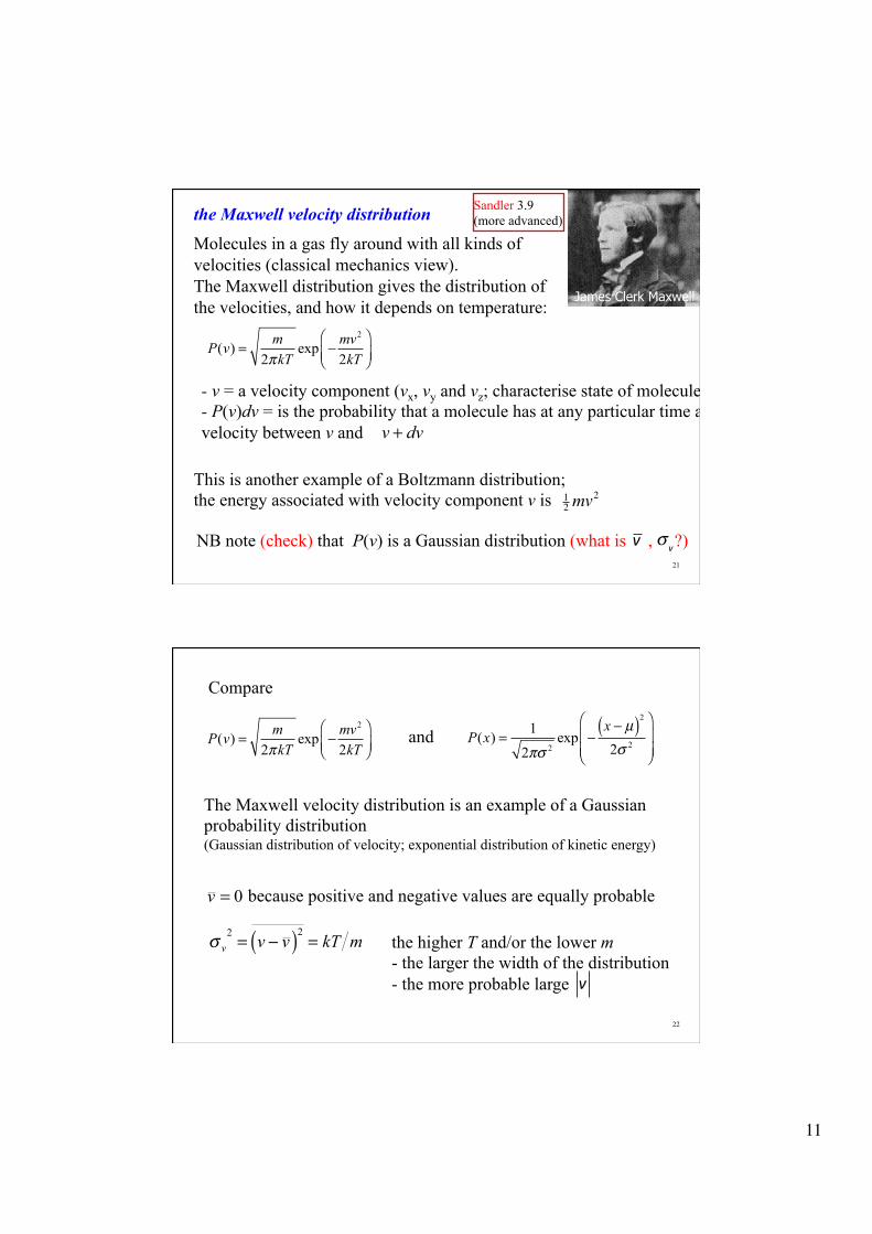
the Maxwell velocity distribution

Molecules in a gas fly around with all kinds of velocities (classical mechanics view). The Maxwell distribution gives the distribution of the velocities, and how it depends on temperature:

P(v) = m2πkT

exp − mv2

2kT⎛⎝⎜

⎞⎠⎟

- v = a velocity component (vx, vy and vz; characterise state of molecule) - P(v)dv = is the probability that a molecule has at any particular time a velocity between v and

�

v + dv

This is another example of a Boltzmann distribution; the energy associated with velocity component v is 12mv

2

Sandler 3.9 (more advanced)

James Clerk Maxwell

NB note (check) that P(v) is a Gaussian distribution (what is , ?) v σ v

22

The Maxwell velocity distribution is an example of a Gaussian probability distribution (Gaussian distribution of velocity; exponential distribution of kinetic energy)

because positive and negative values are equally probable

�

v = 0

�

σ v2 = v − v ( )2

= kT m

Compare

P(v) = m2πkT

exp − mv2

2kT⎛⎝⎜

⎞⎠⎟

and P(x) = 1

2πσ 2exp −

x − µ( )22σ 2

⎛

⎝⎜⎜

⎞

⎠⎟⎟

the higher T and/or the lower m - the larger the width of the distribution - the more probable large v

12

23

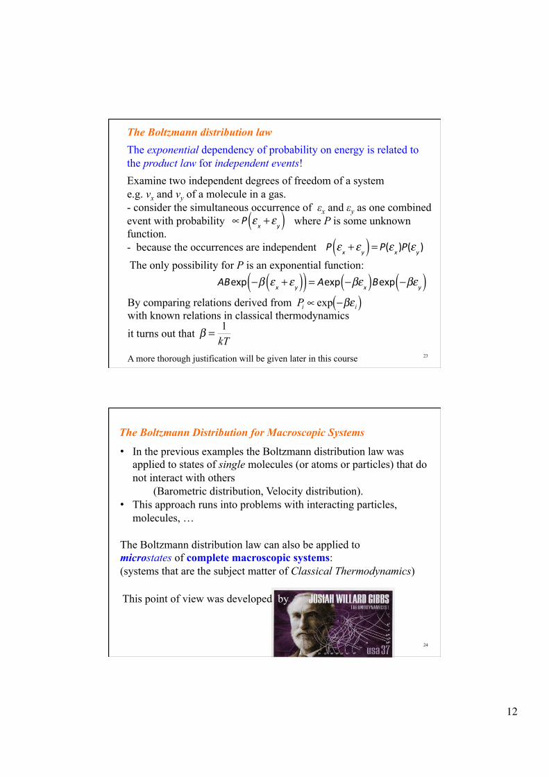
The Boltzmann distribution law

The exponential dependency of probability on energy is related to the product law for independent events!

Examine two independent degrees of freedom of a system e.g. vx and vy of a molecule in a gas. -  consider the simultaneous occurrence of εx and εy as one combined event with probability where P is some unknown function. -  because the occurrences are independent The only possibility for P is an exponential function:

∝P ε x + εy( )P ε x + εy( ) = P(ε x )P(εy )

ABexp −β ε x + εy( )( ) = Aexp −βε x( )Bexp −βεy( )By comparing relations derived from with known relations in classical thermodynamics

it turns out that A more thorough justification will be given later in this course

�

Pi ∝ exp −βε i( )

�

β = 1kT

24

The Boltzmann Distribution for Macroscopic Systems

•  In the previous examples the Boltzmann distribution law was applied to states of single molecules (or atoms or particles) that do not interact with others

(Barometric distribution, Velocity distribution). •  This approach runs into problems with interacting particles,

molecules, …

The Boltzmann distribution law can also be applied to microstates of complete macroscopic systems: (systems that are the subject matter of Classical Thermodynamics)

This point of view was developed by

13

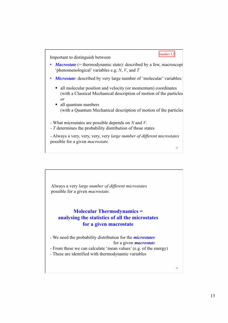
25

Important to distinguish between

•  Macrostate (= thermodynamic state): described by a few, macroscopic, ‘phenomenological’ variables e.g. N, V, and T

•  Microstate: described by very large number of ‘molecular’ variables:

!  all molecular position and velocity (or momentum) coordinates !  (with a Classical Mechanical description of motion of the particles) !  or !  all quantum numbers !  (with a Quantum Mechanical description of motion of the particles)

- What microstates are possible depends on N and V. - T determines the probability distribution of those states

- Always a very, very, very, very large number of different microstates possible for a given macrostate.

Sandler 1.2

26

Molecular Thermodynamics = analysing the statistics of all the microstates

for a given macrostate

Always a very large number of different microstates possible for a given macrostate.

- We need the probability distribution for the microstates for a given macrostate

- From these we can calculate ‘mean values’ (e.g. of the energy) - These are identified with thermodynamic variables

14

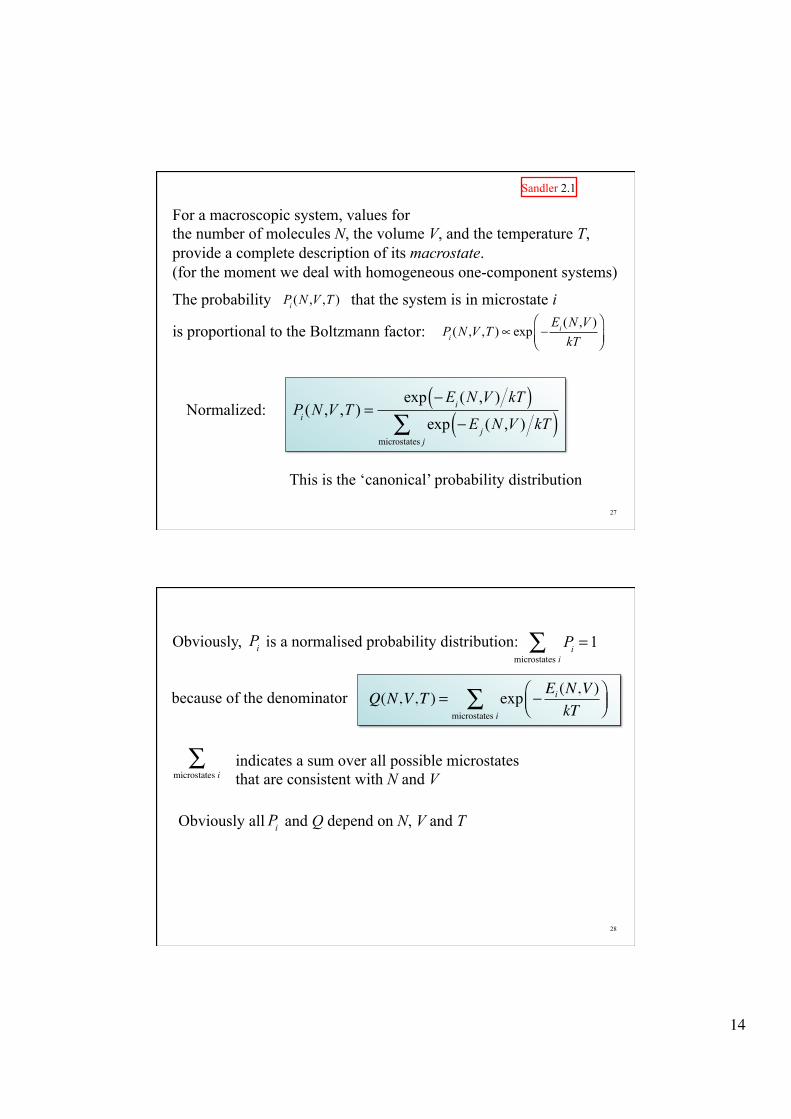
27

For a macroscopic system, values for the number of molecules N, the volume V, and the temperature T, provide a complete description of its macrostate. (for the moment we deal with homogeneous one-component systems)

The probability that the system is in microstate i

is proportional to the Boltzmann factor: Pi (N ,V ,T )∝ exp −Ei (N ,V )kT

⎛⎝⎜

⎞⎠⎟

Pi (N ,V ,T )

Pi (N ,V ,T ) =exp −Ei (N ,V ) kT( )

exp −E j (N ,V ) kT( )microstates j∑

Normalized:

This is the ‘canonical’ probability distribution

Sandler 2.1

Obviously, is a normalised probability distribution:

28

Pi Pimicrostates i∑ =1

Q(N,V,T ) = exp − Ei (N,V )kT

⎛⎝⎜

⎞⎠⎟microstates i

∑

Obviously all and Q depend on N, V and T

because of the denominator

microstates i∑ indicates a sum over all possible microstates

that are consistent with N and V

Pi

15

29

Q(N,V,T ) = exp − Ei

kT⎛⎝⎜

⎞⎠⎟microstates i

∑

is called the (Canonical) Partition Function

in English: in German:

in Dutch: in English sometimes:

We will see that Q is a very important function.

It plays an important role as a “bridge” with Thermodynamics.

“Partition Function” “Zustandsumme” “Toestandsom” “Sum over states”

What thermodynamic function has a special relation with the variables N, V, and T?

30

The internal mechanical energy… (in classical mechanics: the total of all kinetic and potential energies of all the molecules, atoms; in quantum mechanics: the energy level of the quantum state)

of a closed system (N,V,T are fixed)… (NB the macroscopic / thermodynamic state is fixed)

fluctuates in time, around a certain average as the system assumes different microstates over time. Also when the energy of thermodynamic replica’s of the system (same N,V,T) are measured at the same time, the outcome varies.

�

↑E

�

E

�

t →

Sandler 2.2, 3.3

16

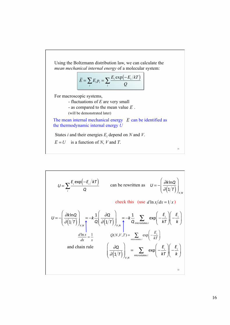
Using the Boltzmann distribution law, we can calculate the mean mechanical internal energy of a molecular system: For macroscopic systems,

- fluctuations of E are very small - as compared to the mean value . (will be demonstrated later)

31

E = Ei pii∑ =

Ei exp −Ei kT( )Qi

∑

�

E

�

E

�

E = U is a function of N, V and T. States i and their energies Ei depend on N and V.

The mean internal mechanical energy can be identified as the thermodynamic internal energy U

32

U =Ei exp −Ei kT( )

Qi∑ can be rewritten as U = − ∂k lnQ

∂ 1 T( )⎛

⎝⎜⎜

⎞

⎠⎟⎟V ,N

d ln x dx =1 xcheck this (use )

U = − ∂k lnQ∂ 1 T( )

⎛

⎝⎜⎜

⎞

⎠⎟⎟V ,N

= −k 1Q

∂Q∂ 1 T( )

⎛

⎝⎜⎜

⎞

⎠⎟⎟V ,N

= −k 1Q

exp −Ei

kT

⎛

⎝⎜⎞

⎠⎟microstates0i∑ −

Ei

k

⎛

⎝⎜⎞

⎠⎟

Q(N ,V ,T ) = exp −EikT

⎛⎝⎜

⎞⎠⎟microstates i

∑d ln xdx

= 1x

and chain rule ∂Q∂ 1 T( )

⎛

⎝⎜⎜

⎞

⎠⎟⎟V ,N

= exp −Ei

kT

⎛

⎝⎜⎞

⎠⎟microstates.i∑ −

Ei

k

⎛

⎝⎜⎞

⎠⎟

?

17

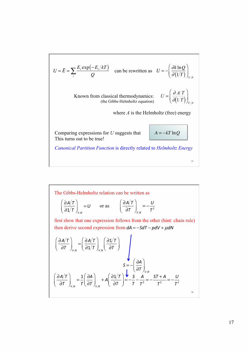
33

U = E =Ei exp −Ei kT( )

Qi∑ can be rewritten as U = − ∂k lnQ

∂ 1 T( )⎛

⎝⎜⎞

⎠⎟V ,N

Known from classical thermodynamics: (the Gibbs-Helmholtz equation)

�

U = ∂ A T∂ 1 T( )

⎛

⎝ ⎜ ⎞

⎠ ⎟ V ,N

where A is the Helmholtz (free) energy

Comparing expressions for U suggests that This turns out to be true!

A = −kT lnQ

Canonical Partition Function is directly related to Helmholtz Energy

34

then derive second expression from dA = −SdT − pdV + µdN

The Gibbs-Helmholtz relation can be written as

or as ∂A T∂1 T

⎛⎝⎜

⎞⎠⎟V ,N

=U∂A T∂T

⎛⎝⎜

⎞⎠⎟V ,N

= − UT 2

first show that one expression follows from the other (hint: chain rule)

∂A T∂T

⎛⎝⎜

⎞⎠⎟V ,N

= ∂A T∂1 T

⎛⎝⎜

⎞⎠⎟V ,N

∂1 T∂T

⎛⎝⎜

⎞⎠⎟

S = − ∂A∂T

⎛⎝⎜

⎞⎠⎟V ,N

∂A T∂T

⎛⎝⎜

⎞⎠⎟V ,N

= 1T

∂A∂T

⎛⎝⎜

⎞⎠⎟V ,N

+ A ∂1 T∂T

⎛⎝⎜

⎞⎠⎟= − S

T− AT 2

= − ST + AT 2

= − UT 2

tomorrow’s tutorial ?

18

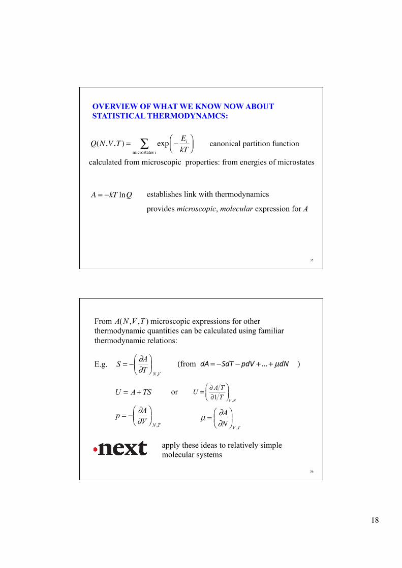
35

A = −kT lnQ

Q(N,V,T ) = exp − Ei

kT⎛⎝⎜

⎞⎠⎟microstates i

∑calculated from microscopic properties: from energies of microstates

canonical partition function

establishes link with thermodynamics

provides microscopic, molecular expression for A

OVERVIEW OF WHAT WE KNOW NOW ABOUT STATISTICAL THERMODYNAMCS:

36

From microscopic expressions for other thermodynamic quantities can be calculated using familiar thermodynamic relations:

E.g.

�

A(N ,V ,T )

�

S = − ∂A∂T

⎛ ⎝ ⎜

⎞ ⎠ ⎟

N ,V

�

U = A + TS

�

p = − ∂A∂V

⎛ ⎝ ⎜

⎞ ⎠ ⎟

N ,T

�

µ = ∂A∂N

⎛ ⎝ ⎜

⎞ ⎠ ⎟

V ,T

(from ) dA = −SdT − pdV + ...+ µdN

apply these ideas to relatively simple molecular systems

or U = ∂A T∂1 T

⎛⎝⎜

⎞⎠⎟V ,N