MTAT.03.244 Software Economics

Workshop 3: Software Cost Estimation

Marlon Dumas

marlon.dumas ät ut . ee

2

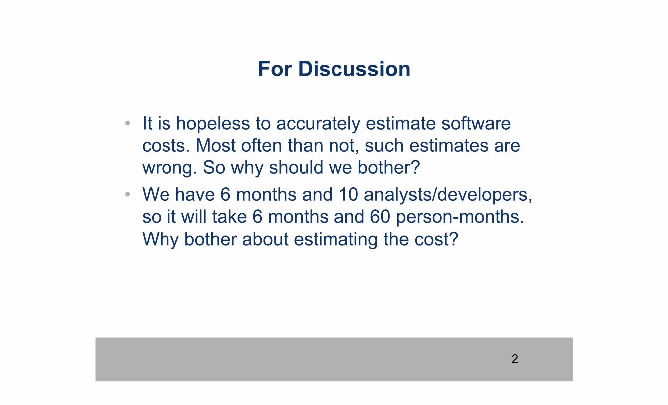
For Discussion

•  It is hopeless to accurately estimate software costs. Most often than not, such estimates are wrong. So why should we bother?

•  We have 6 months and 10 analysts/developers, so it will take 6 months and 60 person-months. Why bother about estimating the cost?

3

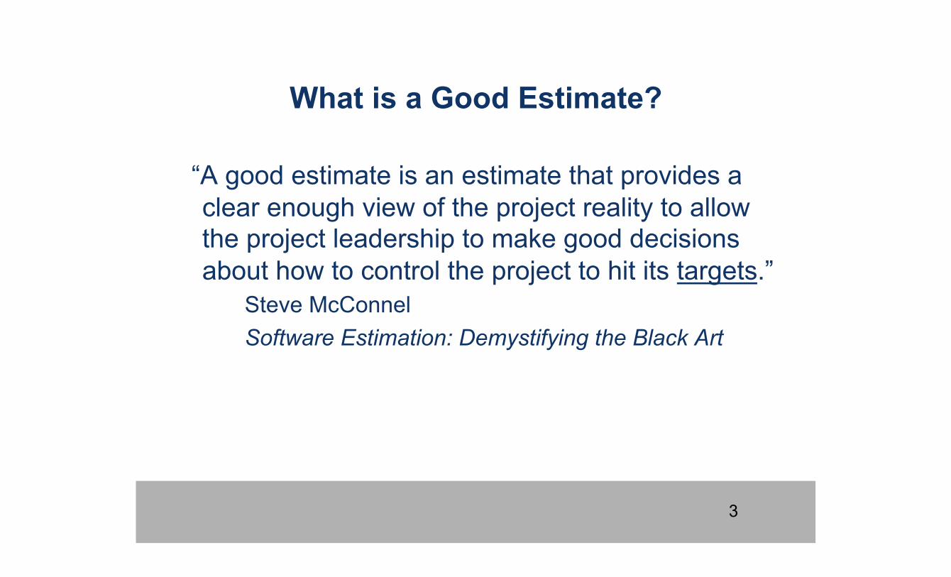
What is a Good Estimate?

“A good estimate is an estimate that provides a clear enough view of the project reality to allow the project leadership to make good decisions about how to control the project to hit its targets.”

Steve McConnel Software Estimation: Demystifying the Black Art

4

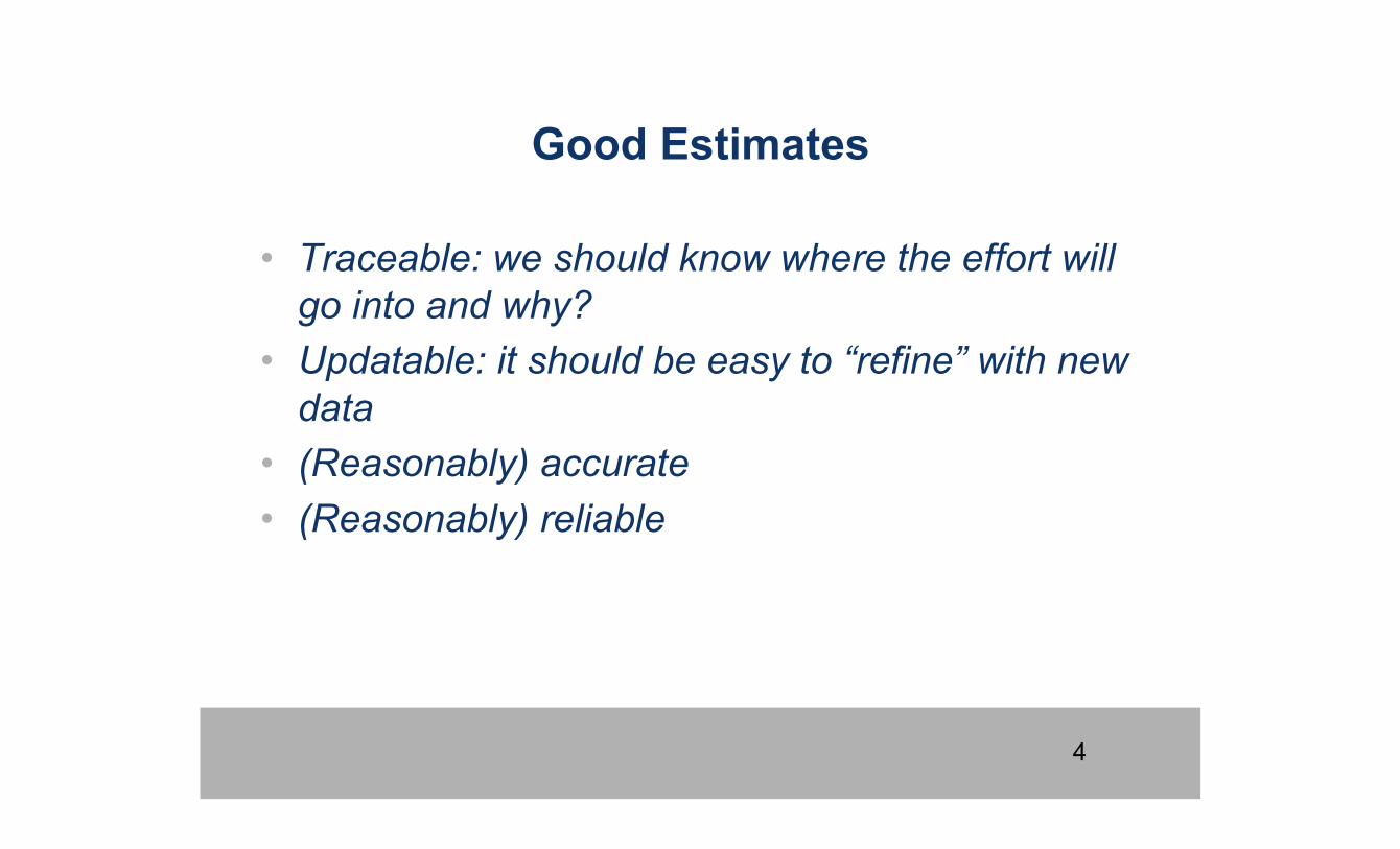
Good Estimates

•  Traceable: we should know where the effort will go into and why?

•  Updatable: it should be easy to “refine” with new data

•  (Reasonably) accurate •  (Reasonably) reliable

5

There are lies, dammed lies and statistics.

•  What about a method to estimate software costs from a high-level architecture, that is: •  within 20% of the actual size 50% of the time •  within 30% of the actual size 66% of the time •  Decomposes effort/cost into four project

phases •  Can we use it and how?

6

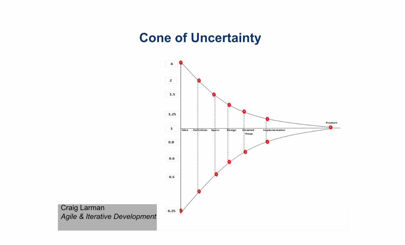
Cone of Uncertainty

Craig Larman Agile & Iterative Development

7

Effort Estimation

•  Parkinson's Law? –  If we have 5 person-years, it will take 5 person-years

•  Estimation by analogy –  This project is 20% more complex than the previous one

•  Expert judgement –  Wideband Delphi –  Planning Poker

8

Wide-Band Delphi

•  Ask each team member their estimate – Apply personal experience, – Look at completed projects, – Extrapolate from modules known to date

•  Collect and share in a meeting: discuss why/how different people made their estimate

•  Repeat •  When stable, Size = (H + 4 X Ave. + L)/6

–  See: http://www.stellman-greene.com/ch03

9

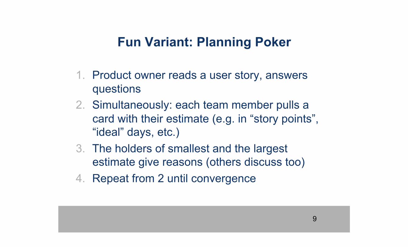
Fun Variant: Planning Poker

1.  Product owner reads a user story, answers questions

2.  Simultaneously: each team member pulls a card with their estimate (e.g. in “story points”, “ideal” days, etc.)

3.  The holders of smallest and the largest estimate give reasons (others discuss too)

4.  Repeat from 2 until convergence

10

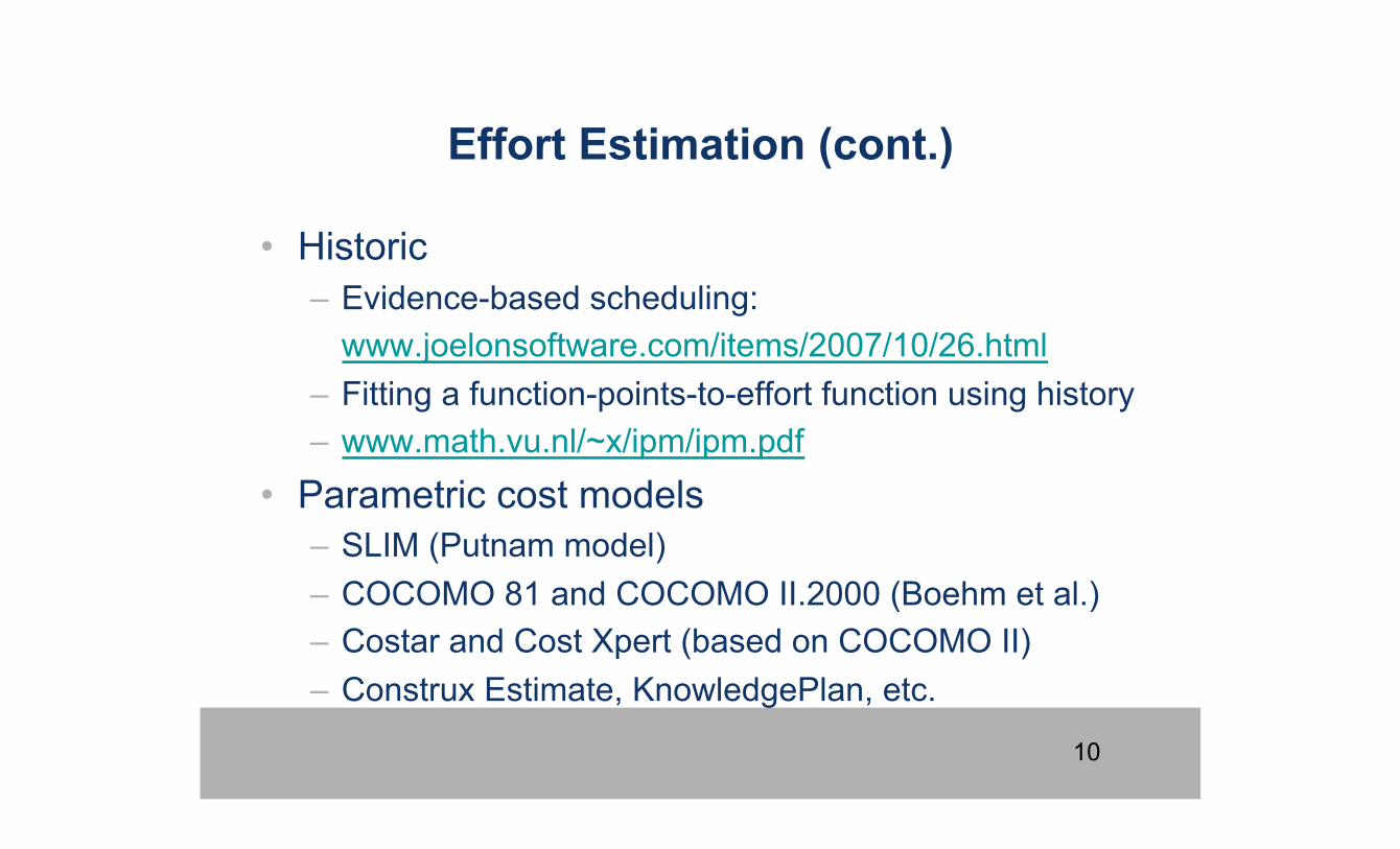
Effort Estimation (cont.)

•  Historic –  Evidence-based scheduling:

www.joelonsoftware.com/items/2007/10/26.html –  Fitting a function-points-to-effort function using history –  www.math.vu.nl/~x/ipm/ipm.pdf

•  Parametric cost models –  SLIM (Putnam model) –  COCOMO 81 and COCOMO II.2000 (Boehm et al.) –  Costar and Cost Xpert (based on COCOMO II) –  Construx Estimate, KnowledgePlan, etc.

11

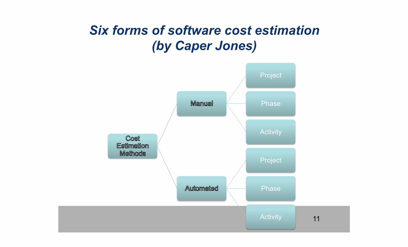
Six forms of software cost estimation (by Caper Jones)

Project

Phase

Activity

Project

Phase

Activity

12

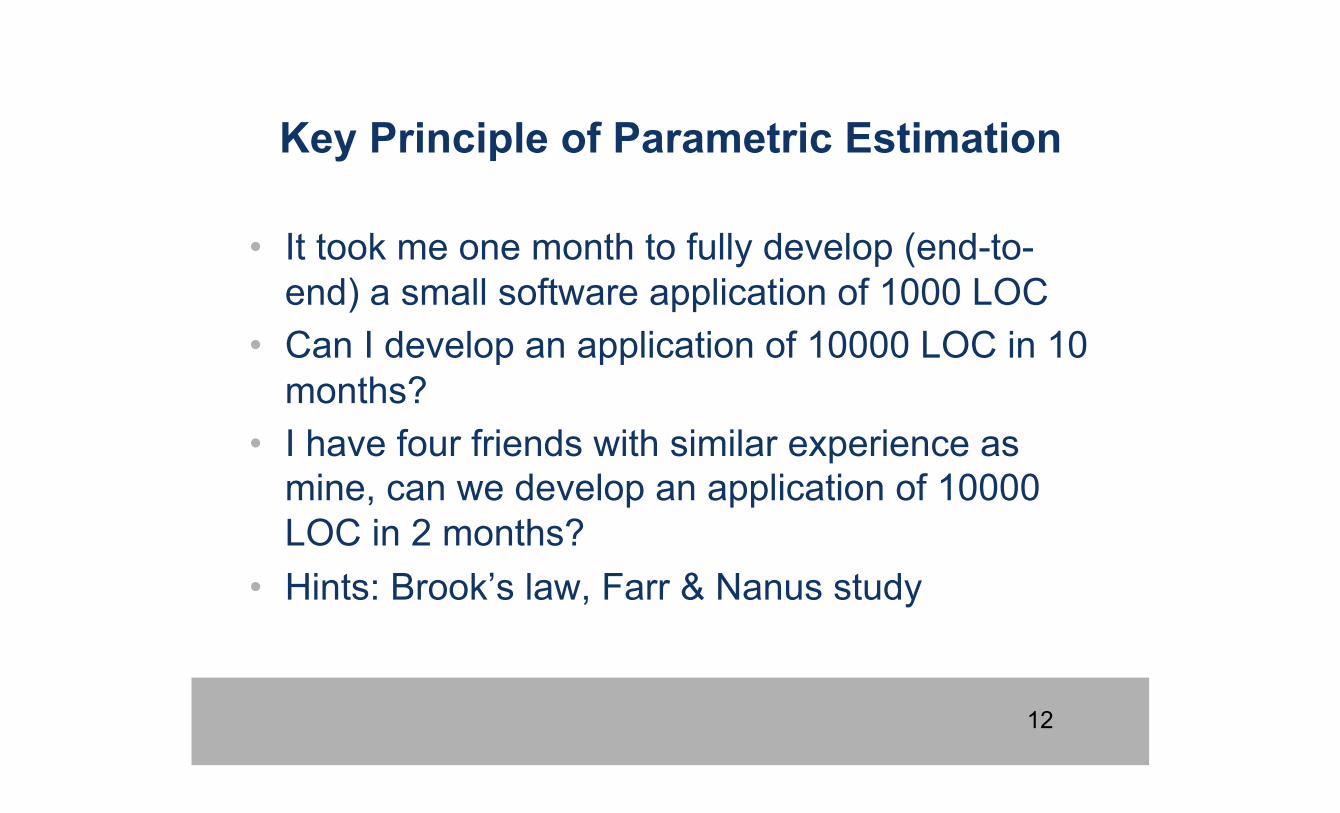
Key Principle of Parametric Estimation

•  It took me one month to fully develop (end-to-end) a small software application of 1000 LOC

•  Can I develop an application of 10000 LOC in 10 months?

•  I have four friends with similar experience as mine, can we develop an application of 10000 LOC in 2 months?

•  Hints: Brook’s law, Farr & Nanus study

13

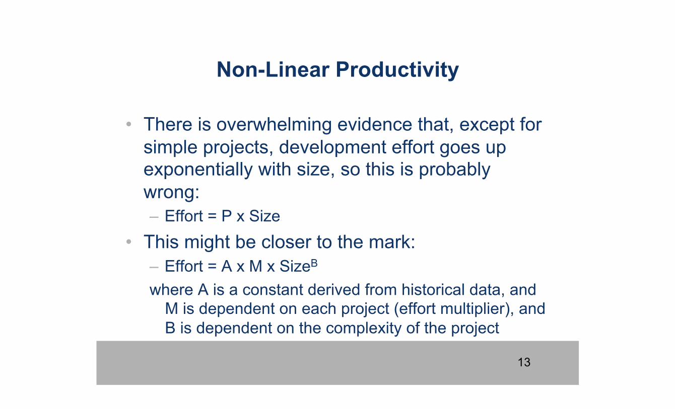
Non-Linear Productivity

•  There is overwhelming evidence that, except for simple projects, development effort goes up exponentially with size, so this is probably wrong: –  Effort = P x Size

•  This might be closer to the mark: –  Effort = A x M x SizeB

where A is a constant derived from historical data, and M is dependent on each project (effort multiplier), and B is dependent on the complexity of the project

14 (c) 2005-08 USC CSSE

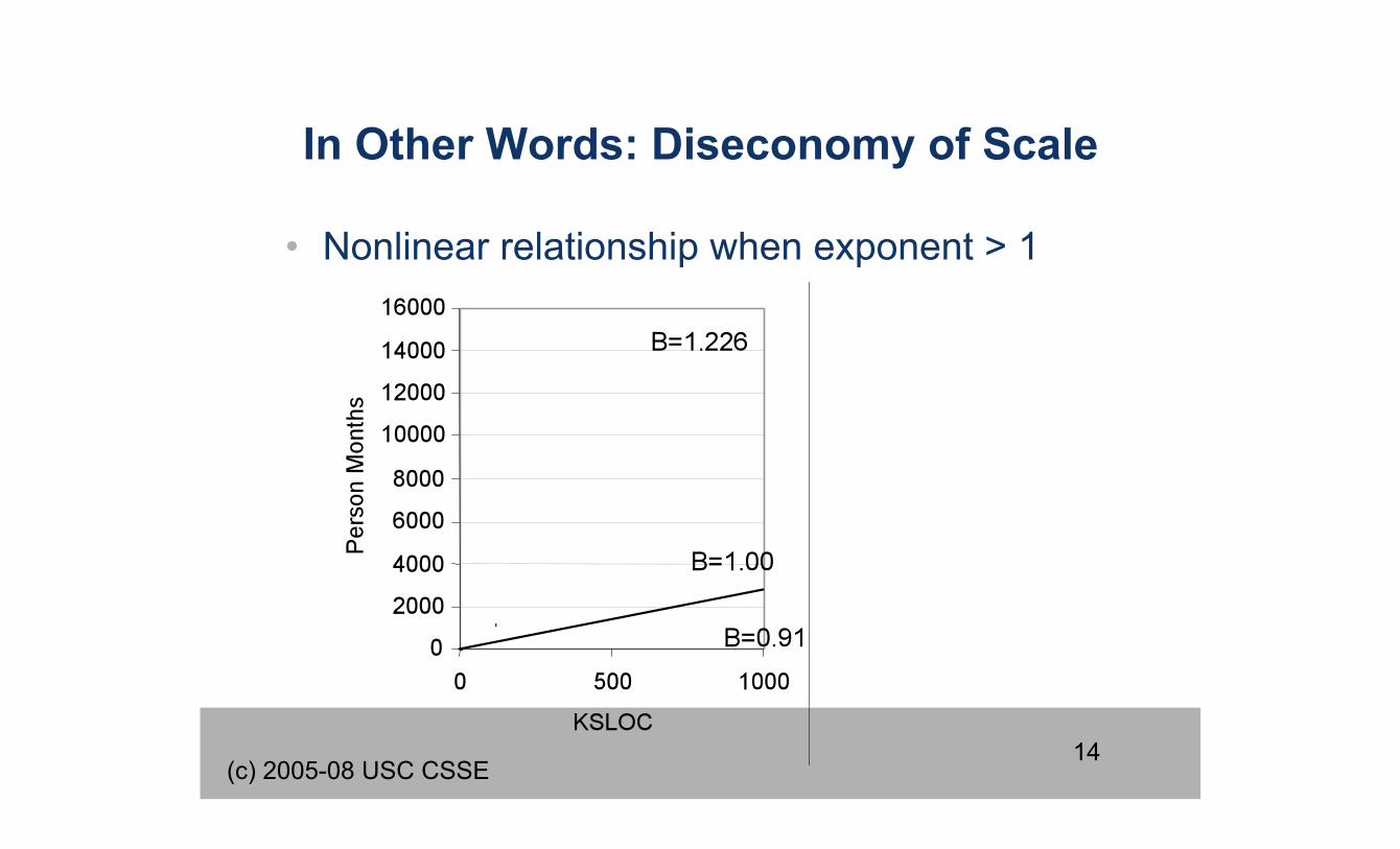
In Other Words: Diseconomy of Scale

•  Nonlinear relationship when exponent > 1

15

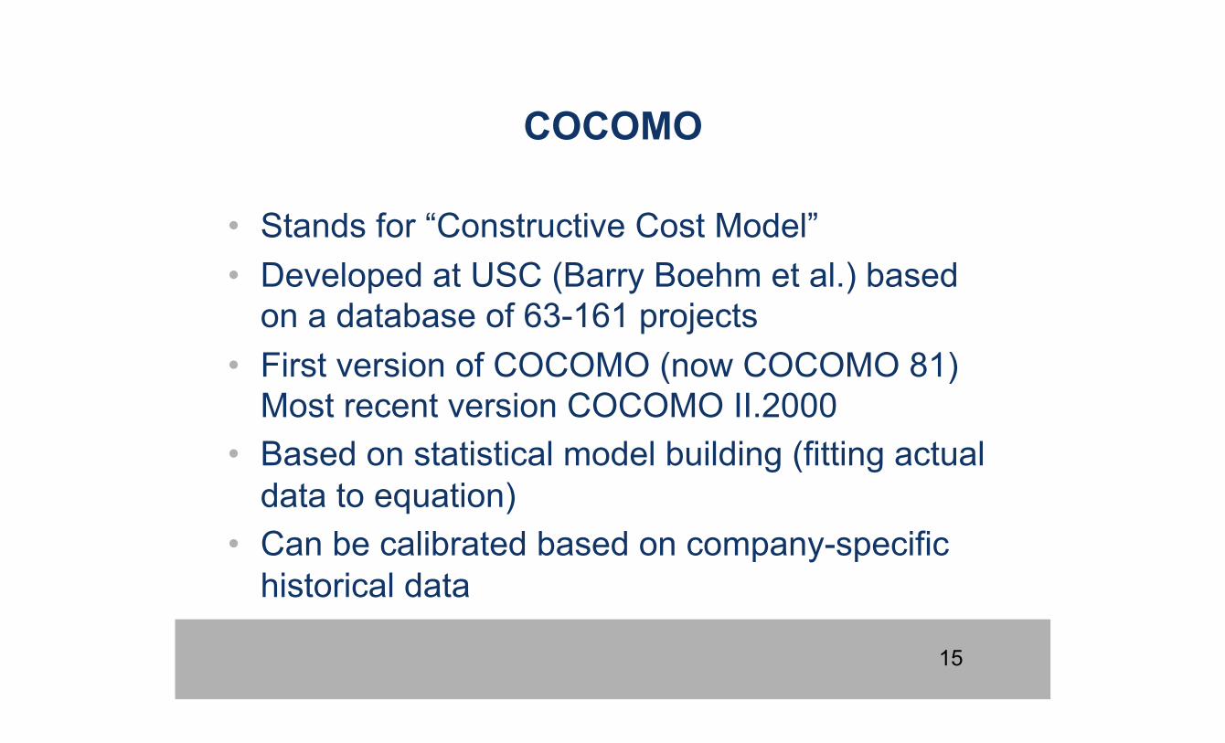
COCOMO

•  Stands for “Constructive Cost Model” •  Developed at USC (Barry Boehm et al.) based

on a database of 63-161 projects •  First version of COCOMO (now COCOMO 81)

Most recent version COCOMO II.2000 •  Based on statistical model building (fitting actual

data to equation) •  Can be calibrated based on company-specific

historical data

16

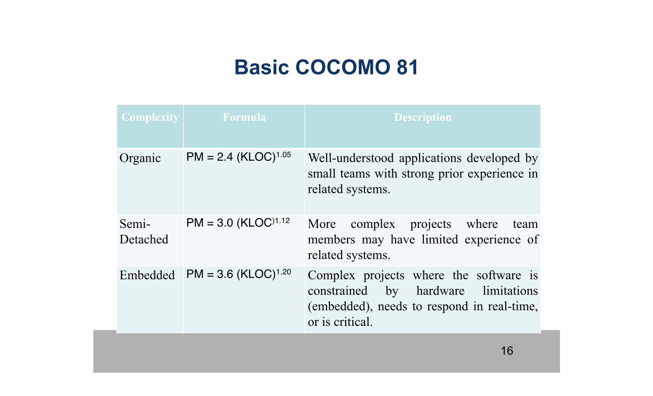
Basic COCOMO 81

Complexity Formula Description

Organic PM = 2.4 (KLOC)1.05 Well-understood applications developed by small teams with strong prior experience in related systems.

Semi-Detached

PM = 3.0 (KLOC)1.12 More complex projects where team members may have limited experience of related systems.

Embedded PM = 3.6 (KLOC)1.20 Complex projects where the software is constrained by hardware limitations (embedded), needs to respond in real-time, or is critical.

17

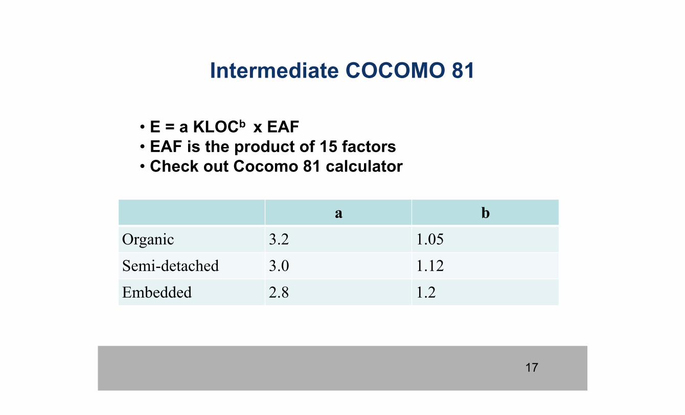
Intermediate COCOMO 81

a b Organic 3.2 1.05 Semi-detached 3.0 1.12 Embedded 2.8 1.2

•  E = a KLOCb x EAF •  EAF is the product of 15 factors •  Check out Cocomo 81 calculator

18

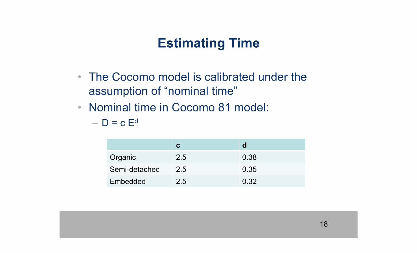
Estimating Time

•  The Cocomo model is calibrated under the assumption of “nominal time”

•  Nominal time in Cocomo 81 model: –  D = c Ed

c d Organic 2.5 0.38 Semi-detached 2.5 0.35 Embedded 2.5 0.32

19

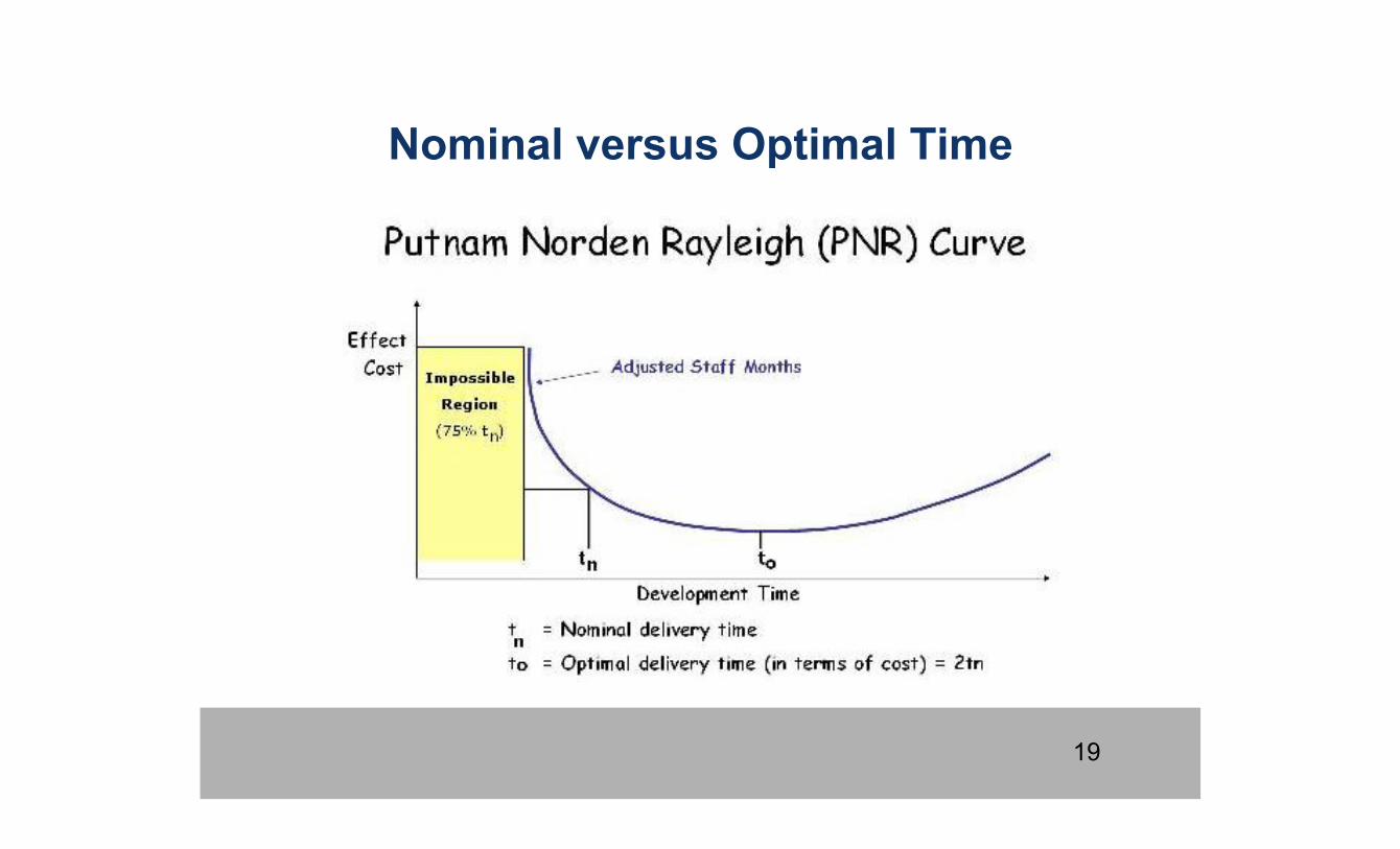
Nominal versus Optimal Time

20

Estimating Size

•  From the early design, we can count FPs •  FPs to LOC can be (roughly) estimated using

“backfiring” •  Capers Jones’s database: > 9000 projects with

both function-points and actual LOC Cobol, –  C, Cobol, Fortran ≈ 100-120 LOC/FP –  Pascal, Ada ≈ 70-90 LOC/FP –  OO Languages ≈ 30 LOC/FP

•  QSM Function Point table: –  http://www.qsm.com/resources/index.html

21

Warm-up Exercise

•  See exercise “Cocomo I” on course web page •  Use the Cocomo 81 calculator (see link on

“Readings” page)

22

COCOMO 81 limitations

•  Over time, Cocomo 81’s database became outdated by new tools, languages and practices

•  Cocomo 81 was designed for the waterfall model, which was largely superseded by incremental, iterative methods

•  Cocomo 81 had only three possible exponents – could not explain for various factors affecting non-linearity of productivity

•  Did not take into account different levels of information available throughout the lifecycle

23

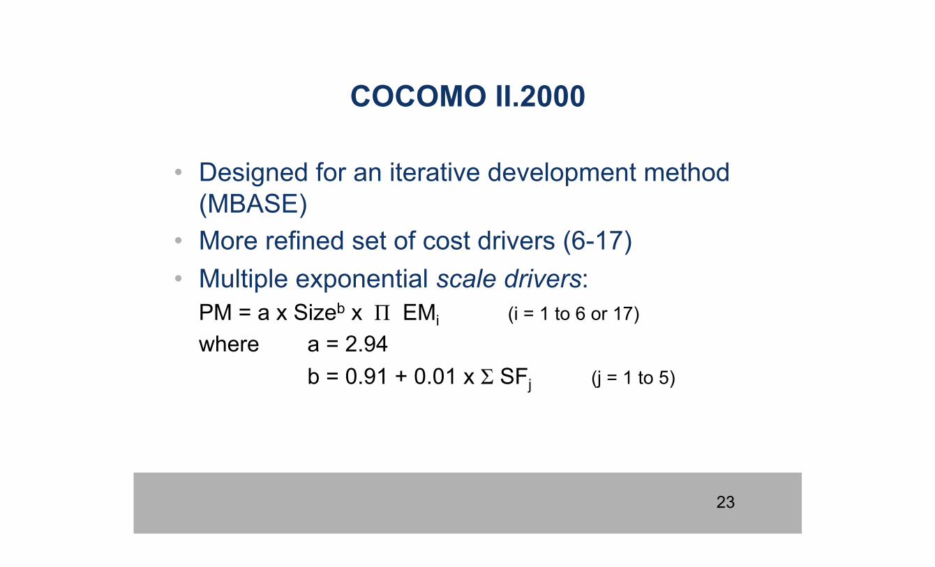
COCOMO II.2000

•  Designed for an iterative development method (MBASE)

•  More refined set of cost drivers (6-17) •  Multiple exponential scale drivers:

PM = a x Sizeb x Π EMi (i = 1 to 6 or 17) where a = 2.94

b = 0.91 + 0.01 x Σ SFj (j = 1 to 5)

24

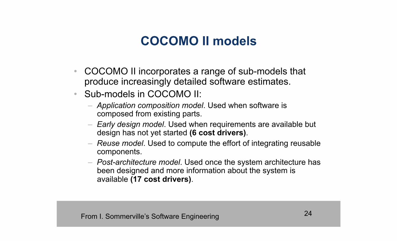
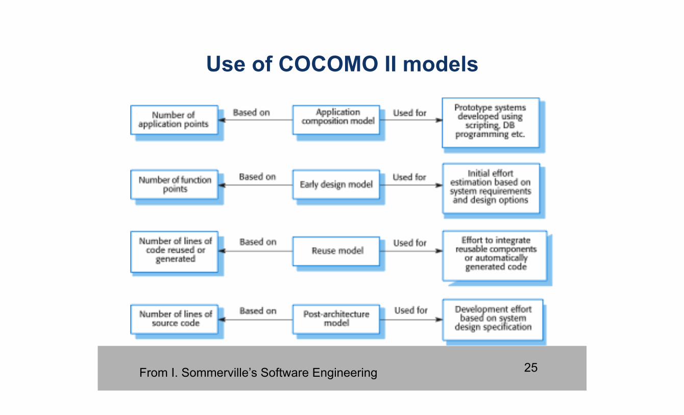
COCOMO II models

•  COCOMO II incorporates a range of sub-models that produce increasingly detailed software estimates.

•  Sub-models in COCOMO II: –  Application composition model. Used when software is

composed from existing parts. –  Early design model. Used when requirements are available but

design has not yet started (6 cost drivers). –  Reuse model. Used to compute the effort of integrating reusable

components. –  Post-architecture model. Used once the system architecture has

been designed and more information about the system is available (17 cost drivers).

From I. Sommerville’s Software Engineering

25

Use of COCOMO II models

From I. Sommerville’s Software Engineering

26 (c) 2005-08 USC CSSE

Cost Factors

•  Significant factors of development cost: –  scale drivers are sources of exponential effort

variation –  cost drivers are sources of linear effort variation

•  product, platform, personnel and project attributes •  effort multipliers associated with cost driver ratings

–  Defined to be as objective as possible •  Each factor is rated between very low and very

high per rating guidelines –  relevant effort multipliers adjust the cost up or down

27 (c) 2005-08 USC CSSE

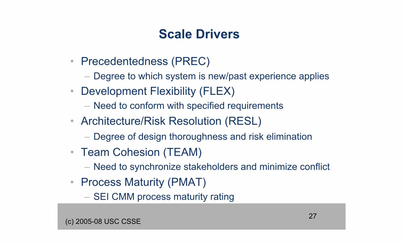
Scale Drivers

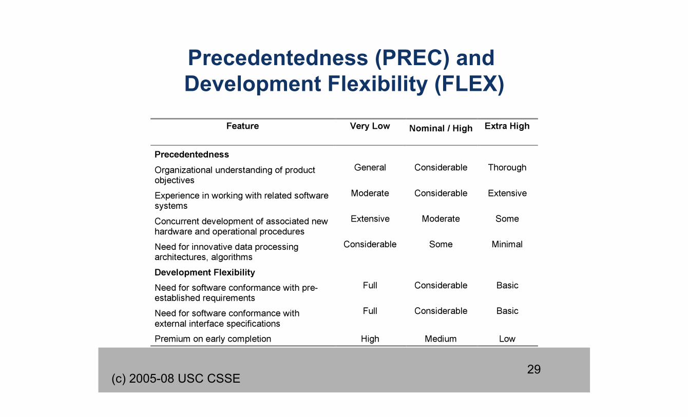
•  Precedentedness (PREC) –  Degree to which system is new/past experience applies

•  Development Flexibility (FLEX) –  Need to conform with specified requirements

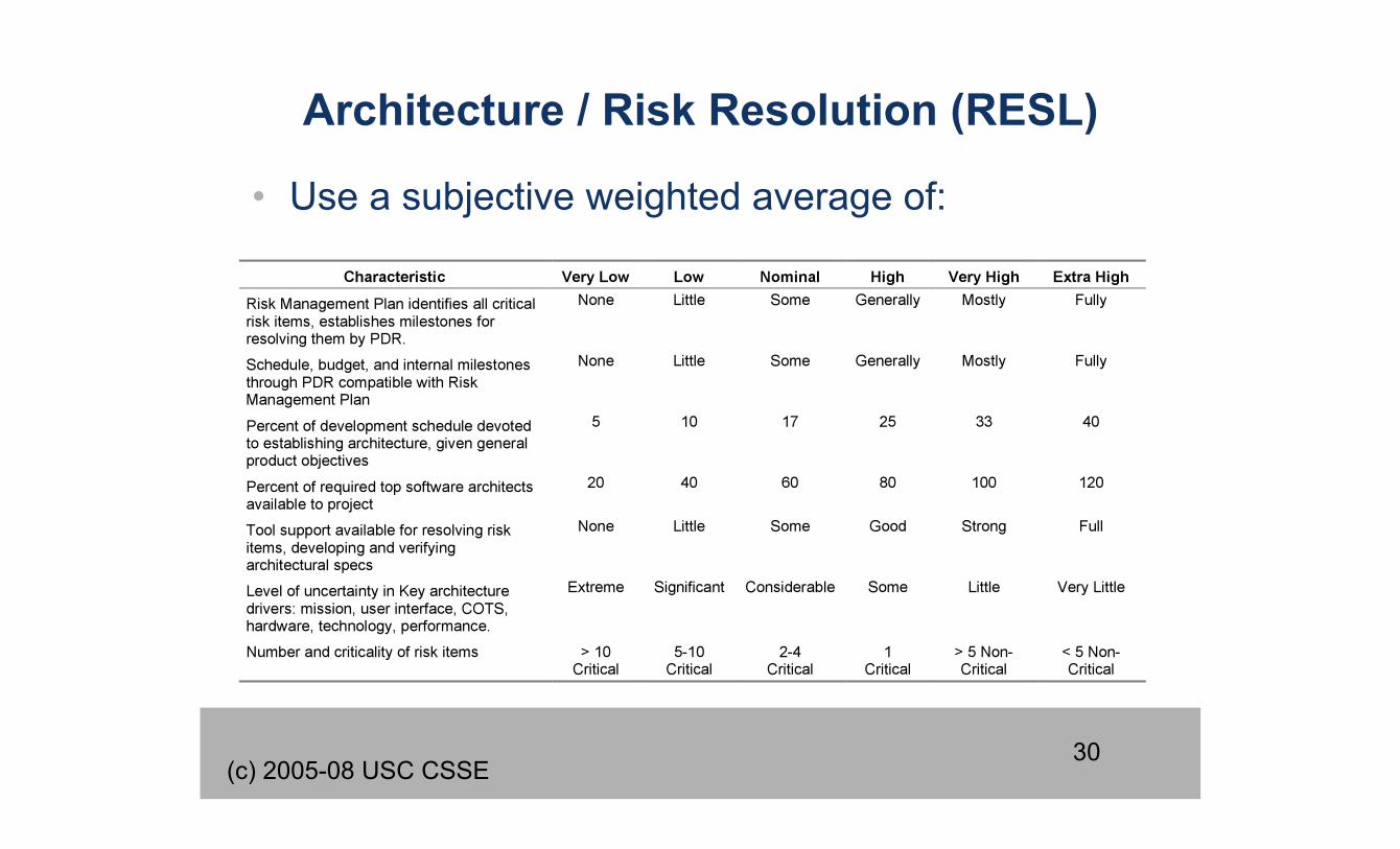
•  Architecture/Risk Resolution (RESL) –  Degree of design thoroughness and risk elimination

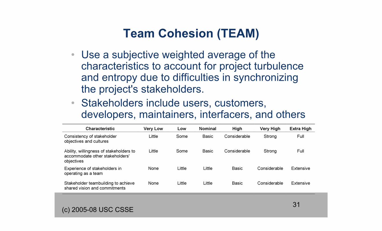
•  Team Cohesion (TEAM) –  Need to synchronize stakeholders and minimize conflict

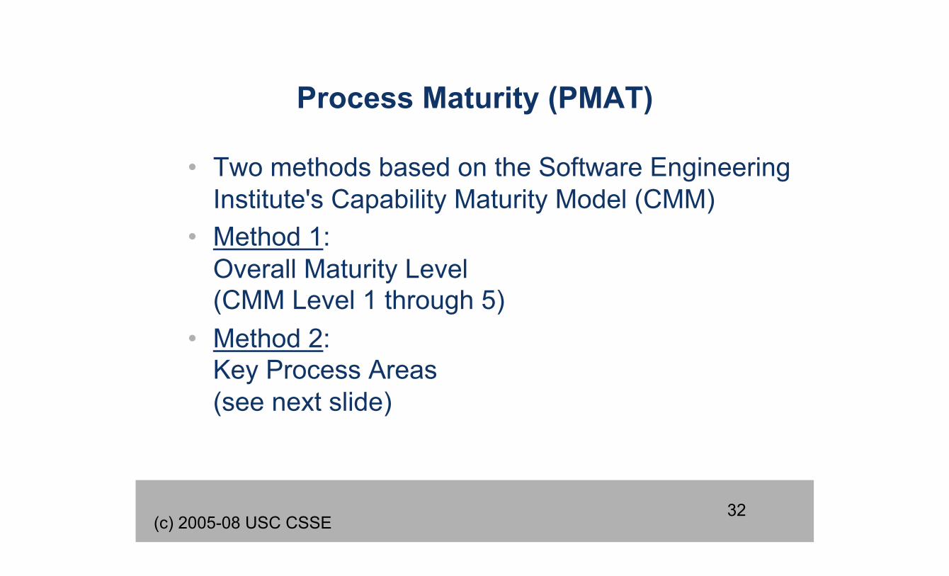
•  Process Maturity (PMAT) –  SEI CMM process maturity rating

28 (c) 2005-08 USC CSSE

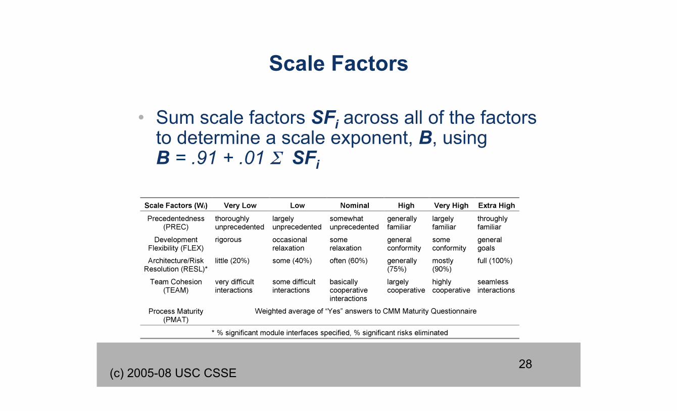
Scale Factors

•  Sum scale factors SFi across all of the factors to determine a scale exponent, B, using B = .91 + .01 Σ SFi

29 (c) 2005-08 USC CSSE

Precedentedness (PREC) and Development Flexibility (FLEX)

30 (c) 2005-08 USC CSSE

Architecture / Risk Resolution (RESL)

•  Use a subjective weighted average of:

31 (c) 2005-08 USC CSSE

Team Cohesion (TEAM) •  Use a subjective weighted average of the

characteristics to account for project turbulence and entropy due to difficulties in synchronizing the project's stakeholders.

•  Stakeholders include users, customers, developers, maintainers, interfacers, and others

32 (c) 2005-08 USC CSSE

Process Maturity (PMAT)

•  Two methods based on the Software Engineering Institute's Capability Maturity Model (CMM)

•  Method 1: Overall Maturity Level (CMM Level 1 through 5)

•  Method 2: Key Process Areas (see next slide)

33 (c) 2005-08 USC CSSE

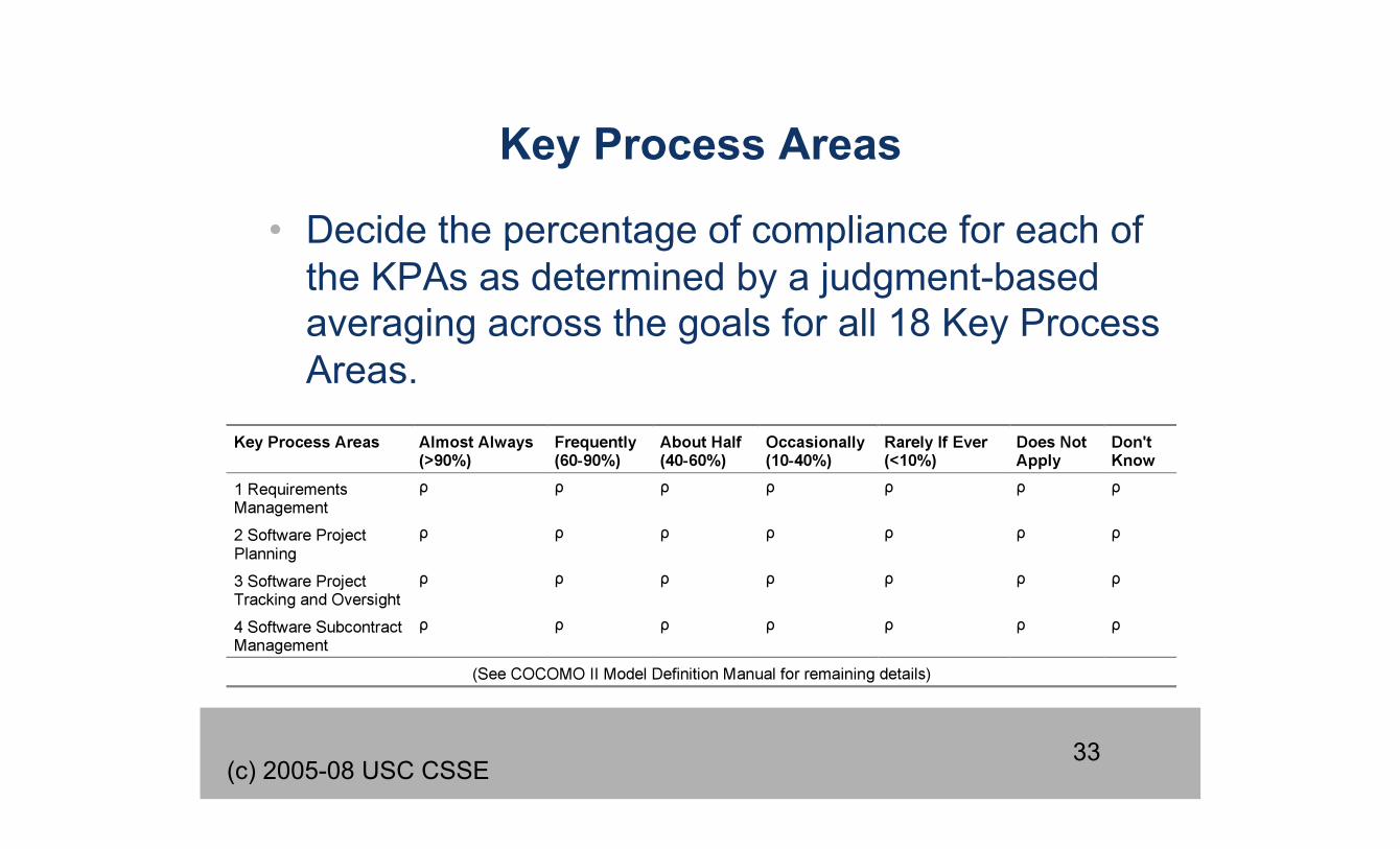
Key Process Areas

•  Decide the percentage of compliance for each of the KPAs as determined by a judgment-based averaging across the goals for all 18 Key Process Areas.

34

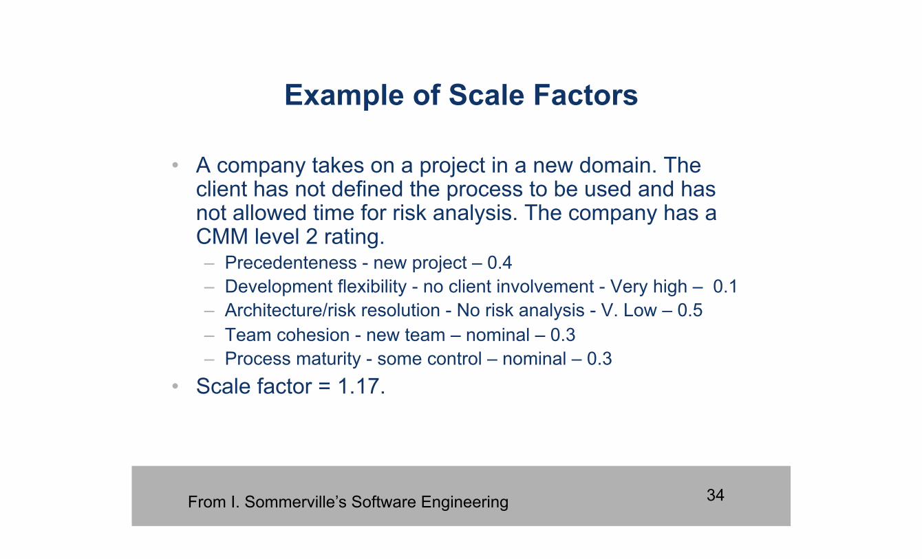
•  A company takes on a project in a new domain. The client has not defined the process to be used and has not allowed time for risk analysis. The company has a CMM level 2 rating. –  Precedenteness - new project – 0.4 –  Development flexibility - no client involvement - Very high – 0.1 –  Architecture/risk resolution - No risk analysis - V. Low – 0.5 –  Team cohesion - new team – nominal – 0.3 –  Process maturity - some control – nominal – 0.3

•  Scale factor = 1.17.

Example of Scale Factors

From I. Sommerville’s Software Engineering

35 (c) 2005-08 USC CSSE

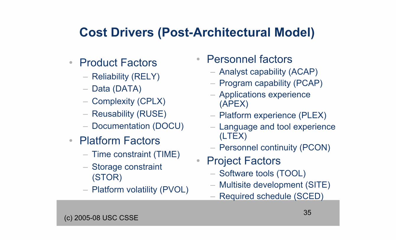
Cost Drivers (Post-Architectural Model)

•  Product Factors –  Reliability (RELY) –  Data (DATA) –  Complexity (CPLX) –  Reusability (RUSE) –  Documentation (DOCU)

•  Platform Factors –  Time constraint (TIME) –  Storage constraint

(STOR) –  Platform volatility (PVOL)

•  Personnel factors –  Analyst capability (ACAP) –  Program capability (PCAP) –  Applications experience

(APEX) –  Platform experience (PLEX) –  Language and tool experience

(LTEX) –  Personnel continuity (PCON)

•  Project Factors –  Software tools (TOOL) –  Multisite development (SITE) –  Required schedule (SCED)

36 (c) 2005-08 USC CSSE

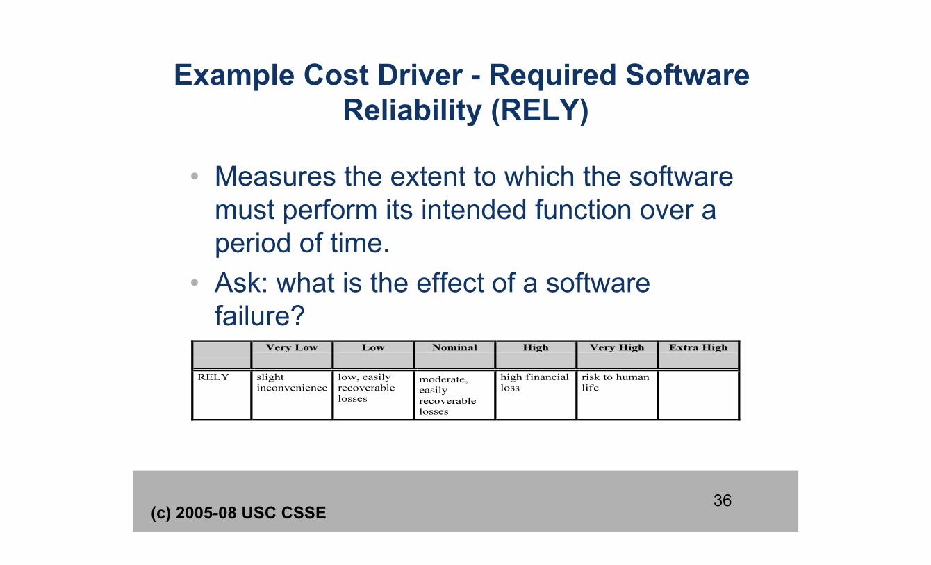
Example Cost Driver - Required Software Reliability (RELY)

•  Measures the extent to which the software must perform its intended function over a period of time.

•  Ask: what is the effect of a software failure?

37 (c) 2005-08 USC CSSE

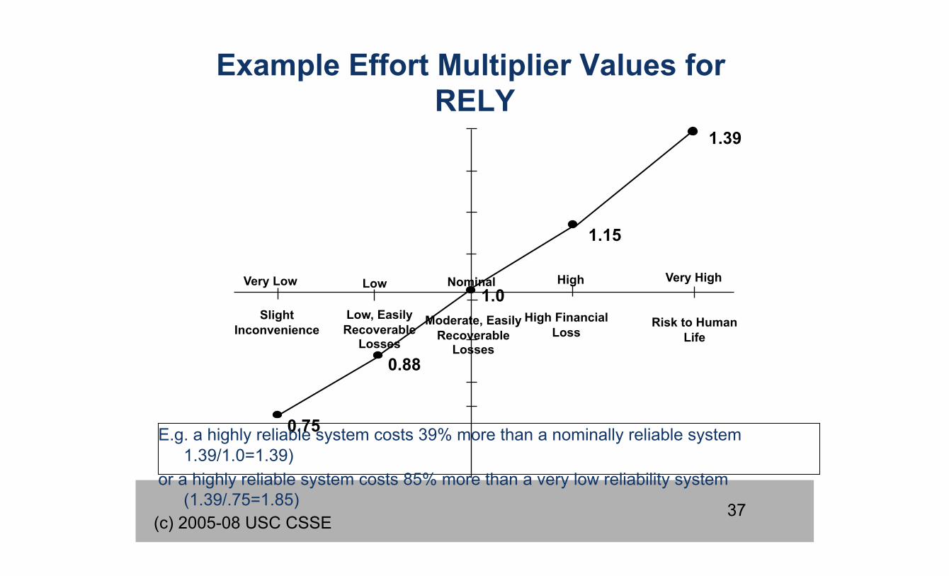
Example Effort Multiplier Values for RELY

Very Low Low High Very High

Slight Inconvenience

Low, Easily Recoverable

Losses

High Financial Loss

Risk to Human Life

1.15

0.75

0.88

1.39

1.0 Moderate, Easily

Recoverable Losses

Nominal

E.g. a highly reliable system costs 39% more than a nominally reliable system 1.39/1.0=1.39)

or a highly reliable system costs 85% more than a very low reliability system (1.39/.75=1.85)

38

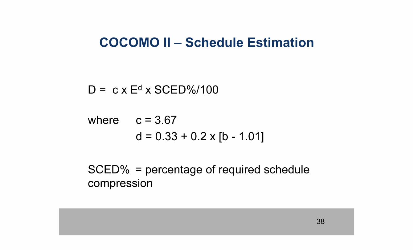
COCOMO II – Schedule Estimation

D = c x Ed x SCED%/100

where c = 3.67

d = 0.33 + 0.2 x [b - 1.01]

SCED% = percentage of required schedule compression

39

Cocomo II Exercise

•  See separate handout •  Use COCOMO II Data Sheet, Model Definition

Manual and online cost Cocomo II calculator (see list of Cocomo Resources under the course’s “Readings” page)

40

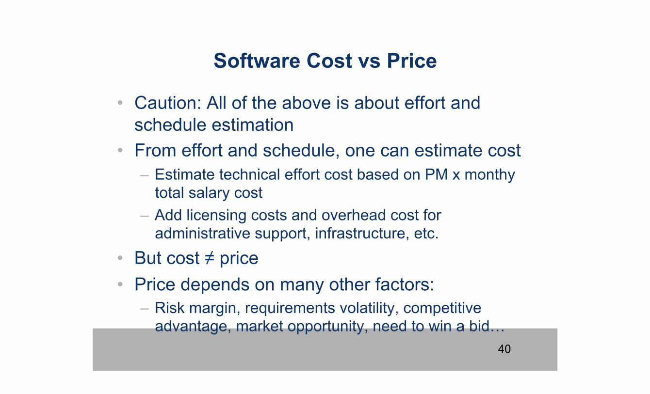
Software Cost vs Price

•  Caution: All of the above is about effort and schedule estimation

•  From effort and schedule, one can estimate cost –  Estimate technical effort cost based on PM x monthy

total salary cost –  Add licensing costs and overhead cost for

administrative support, infrastructure, etc. •  But cost ≠ price •  Price depends on many other factors:

–  Risk margin, requirements volatility, competitive advantage, market opportunity, need to win a bid…

41

Final Word of Caution

•  COCOMO and similar models are just MODELS •  COCOMO comes calibrated by a set of projects

that might not reflect a particular project’s context

•  Should be combined with expert assessment – for example, combine Cocomo with estimates based on the Work Breakdown Structures

•  Cost estimation should be followed by continuous cost control (more on this next week)

42

Re: Homework 1

•  Effort and schedule estimation can be done: –  Using Cocomo II (post-architectural).

•  Explain your choice of cost and scale drivers

–  If small system: Wideband Delphi or planning poker over each individual feature

•  Provide table of feature and estimate in person-days

•  Be ready to answer this question: Is the estimate credible/realistic?