MSEG 803Equilibria in Material Systems

6: Phase space and microstates

Prof. Juejun (JJ) Hu

hujuejun@udel.edu

logS k W

Ludwig Boltzmann

(1844-1906)

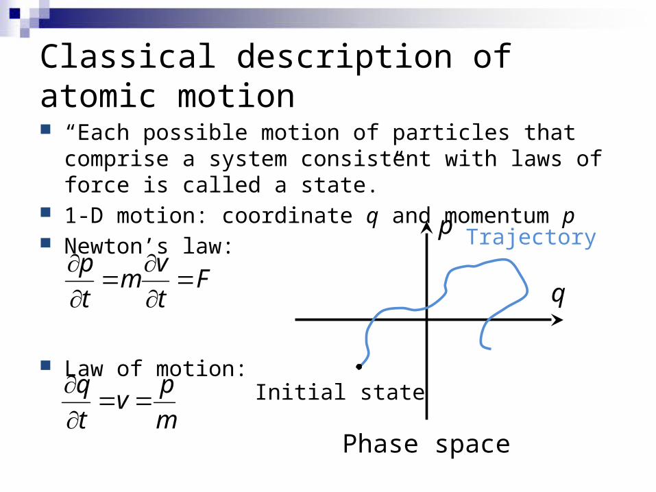
“Each possible motion of particles that comprise a system consistent with laws of force is called a state.”

1-D motion: coordinate q and momentum p Newton’s law:

Law of motion:

p vm F

t t

q pv

t m

Classical description of atomic motion

p

q

Phase space

Initial state

Trajectory

Classical description of atomic motion

For a system consisting of N particles free to move in 3-D space, the phase space has 6N coordinates

In classical mechanics, all particles are distinguishable Newton’s law:

Law of motion:

i ip vm F

t t

i ii

q pv

t m

p

q

Phase space

Initial state

Trajectory

Quantum mechanical description

Single particle quantum mechanical states are represented by a vector (or a wave function Y )

Normalization condition: Physical observables are represented by Hermitian

operators whose eigenvectors form a complete set

x xPosition:

xp i

x

Momentum:

Energy (Hamiltonian): E it

| 1

2

2

2H V

m

Quantum mechanical description

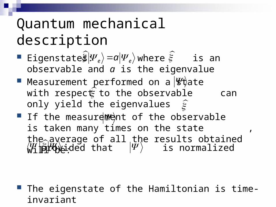
Eigenstates: where is an observable and a is the eigenvalue

Measurement performed on a state with respect to the observable can only yield the eigenvalues

If the measurement of the observable is taken many times on the state , the average of all the results obtained will be:

The eigenstate of the Hamiltonian is time-invariant

e ea

provided that is normalized

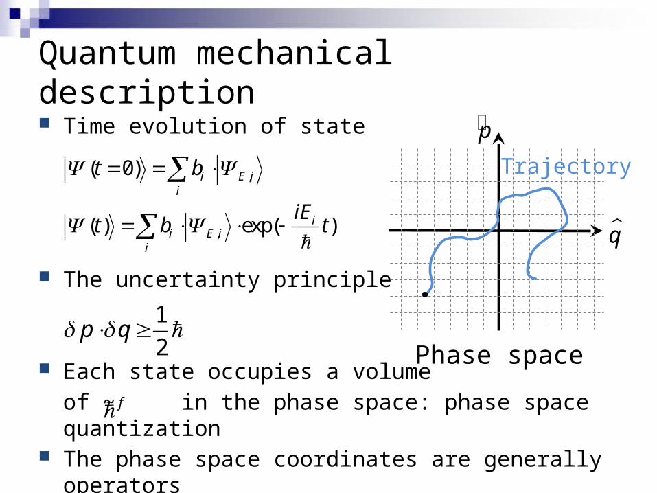
Quantum mechanical description Time evolution of state

The uncertainty principle

Each state occupies a volume

of ~ in the phase space: phase space quantization The phase space coordinates are generally operators

,( 0) i E ii

t b

,( ) exp( )ii E i

i

iEt b t

Phase space

p

q

Trajectory

1

2p q

f

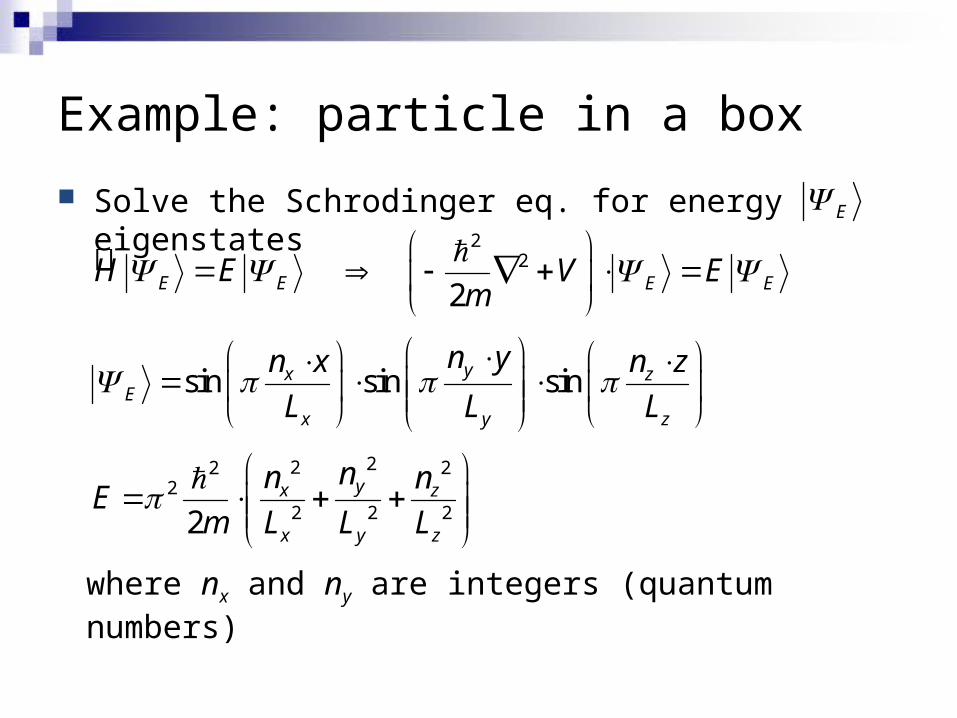
Example: particle in a box

Solve the Schrodinger eq. for energy eigenstates E

E EH E

22

2 E EV Em

sin sin sinyx zE

x y z

n yn x n z

L L L

22 222

2 2 22yx z

x y z

nn nE

m L L L

where nx and ny are integers (quantum numbers)

Comparing classical and quantum descriptions

Trajectory in phase space

Each state has well-defined p and q (a geometric point)

Local density of states in the phase space is infinite (or an arbitrary constant), i.e. the phase space is continuous

Particles are distinguishable

ip Ft

i iq p

t m

Classical mechanics

Trajectory in phase space

Each state’s p and q satisfies the uncertainty principle:

The phase space is quantized; each state occupies a volume of ~

Identical particles

Quantum mechanics

,( 0) i E ii

t b

,( ) exp( )ii E i

i

iEt b t

1 2p q

Statistical ensemble

An idealization consisting of a large number of mental copies of a system, considered all at once, each of which represents a possible state that the real system might be in

Fundamental postulate: given an isolated system in equilibrium, it is found with equal probability in each of its accessible microstates (microcanonical ensemble)

Example: particle spin in a magnetic field H

3 particle system, each with spin ½ Spin can be (½) up or down (-½), corresponding to

magnetic moment m0 or - m0

State # Particle 1 Particle 2 Particle 3 Total M Energy

1 1/2 1/2 1/2 1.5 m0 3 m0H

2 1/2 1/2 -1/2 0.5 m0 m0H

3 1/2 -1/2 1/2 0.5 m0 m0H

4 -1/2 1/2 1/2 0.5 m0 m0H

5 1/2 -1/2 -1/2 -0.5 m0 - m0H

6 -1/2 -1/2 1/2 -0.5 m0 - m0H

7 -1/2 1/2 -1/2 -0.5 m0 - m0H

8 -1/2 -1/2 -1/2 -1.5 m0 -3 m0H

Example: simple 1-D harmonic oscillator

Energy:

States with an energy between E and E + dE fall on an eclipse in the phase space

All of these states are equally accessible

E 21

2kx

21

2

p

m

KineticPotential

x

x

p

E

E + dE dx

B1

B2

dx

Area A is larger than B1 and B2 combined: the system is more likely to be found in the states within area A

A

Relating macroscopic properties with probability distribution of microscopic states

Probability of finding the system in states with the desired property (in a microcanonical ensemble):

Macroscopic parameter X is calculated by integration of summation over the entire phase space:

ii

i N

NP

Total number of states (systems in the ensemble)

# of states (systems) with the desired property

i iX X PX

i iX X PX

Classical: continuous phase space

Quantum: quantized phase space

Density of states

: number of states having energy between E and E + dE

: number of states having energy less than E

For a system with f degrees of freedom

( )E

( )E

( ) ( ) ( )d

E E dE E dEdE

0ln ( ) ln2

fE E E

( )d

E dEdE

Density of states (DOS): ( )d

E dEdE

0ln ( ) ln2

fE E E

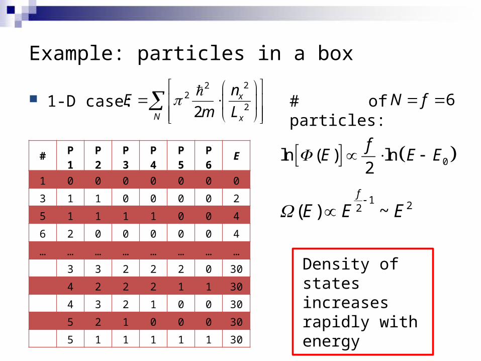
Example: particles in a box

1-D case:22

222x

N x

nE

m L

6N f # of particles:

# P 1 P 2 P 3 P 4 P 5 P 6 E

1 0 0 0 0 0 0 0

3 1 1 0 0 0 0 2

5 1 1 1 1 0 0 4

6 2 0 0 0 0 0 4

… … … … … … … …

3 3 2 2 2 0 30

4 2 2 2 1 1 30

4 3 2 1 0 0 30

5 2 1 0 0 0 30

5 1 1 1 1 1 30

0ln ( ) ln2

fE E E

1 22( ) ~f

E E E

Density of states increases rapidly with energy

Example: classical ideal gas

Consider monatomic gas: Ideal gas consists of non-interacting particles:

kinetic potential intraE E E E

0intraE 0potentialE

2 2 22

2 2x y z

kineticN N

p p ppE E

m m

px

py

R

Example: classical ideal gas (cont’d)2 2 22

2 2x y z

kineticN N

p p ppE E

m m

px

py

R

1 1 1 ,1 ,1 ,1 ,

1 2 ,1 ,1 ,1 ,

,1 ,1 ,1 ,

( ) ... ...

... ...

...

E dE

N N N x y z z NE

E dE

N x y z z NE

R dRNx y z z NR

E dx dy dz dx dy dz dp dp dp dp

dV dV dV dp dp dp dp

V dp dp dp dp

122R mE

33 1 2 2( ) ~

N fN N N NE V R V E V E

DOS is determined by external parameters

Ideal gas: where B is a constant independent of V and E

Generally, energy levels of a system is a function of the external paramaters:

where xi are external parameters of the system (extensive or intensive state variables)

Example: energy levels in a magnetic material depends on its volume and applied field

3

2( ) ( , )N

NE BV E f E V

1 2( ) ( , , ,..., )nE f E x x x