MSE Working Papers WORKING PAPER 124/2015 · PDF fileDeterminants of Energy and Co2 Emission...
32
Pranab Mukhopadhyay Vanessa da Costa MADRAS SCHOOL OF ECONOMICS Gandhi Mandapam Road Chennai 600 025 India September 2015 RECREATIONAL VALUE OF COASTAL AND MARINE ECOSYSTEMS IN INDIA: A PARTIAL ESTIMATE WORKING PAPER 124/2015
Transcript of MSE Working Papers WORKING PAPER 124/2015 · PDF fileDeterminants of Energy and Co2 Emission...
Pranab Mukhopadhyay Vanessa da Costa
MADRAS SCHOOL OF ECONOMICSGandhi Mandapam Road
Chennai 600 025 India
September 2015
RECREATIONAL VALUE OF COASTAL AND MARINE ECOSYSTEMS IN INDIA:
A PARTIAL ESTIMATE
MSE Working Papers
Recent Issues
* Working Paper 112/2015Health Shocks and Short-Term Consumption GrowthSowmya Dhanaraj
* Working Paper 113/2015Efficiency in Elementary Education in Urban India: An Exploratory Analysis Using DeaBrijesh C. Purohit
* Working Paper 114/2015Price Rigidity, Inflation And The Distribution Of Relative Price ChangesSartaj Rasool Rather, S. Raja Sethu Durai and M. Ramachandran
* Working Paper 115/2015Money and Inflation: Evidence from P-Star ModelSunil Paul, Sartaj Rasool Rather and M. Ramachandran
* Working Paper 116/2015Determinants of Energy and Co2 Emission Intensities: A Study of Manufacturing Firms in IndiaSantosh K. Sahu and Deepanjali Mehta
* Working Paper 117/2015Impact of Water and Sanitation on Selected Water Borne Diseases in IndiaBrijesh C. Purohit
* Working Paper 118/2015Health Shocks and Inter-Generational Transmission of InequalitySowmya Dhanaraj
* Working Paper 119/2015Productivity, Energy Intensity and Output: A Unit Level Analysis of the Indian Manufacturing SectorSantosh K. Sahu and Himani Sharma
* Working Paper 120/2015Health Shocks and Coping Strategies: State Health Insurance Scheme of Andhra Pradesh, IndiaSowmya Dhanaraj
* Working Paper 121/2015Efficiency in Education Sector: A Case of Rajasthan State (India)Brijesh C Purohit
* Working Paper 122/2015Mergers and Acquisitions in the Indian Pharmaceutical SectorSantosh Kumar Sahu and Nitika Agarwal
* Working Paper 123/2015Analyzing the Water Footprint of Indian Dairy IndustryZareena B. Irfan and Mohana Mondal
* Working papers are downloadable from MSE website http://www.mse.ac.in
$ Restricted circulation
WORKING PAPER 124/2015
i
Recreational Value of Coastal and Marine Ecosystems in India:A Partial Estimate
Pranab Mukhopadhyay Department of Economics, Goa University, Goa and Visiting Scholars, Madras
School of Economics [email protected]
and
Vanessa da Costa Department of Economics, Goa University, Goa and Visiting Scholars, Madras
School of Economics
ii
WORKING PAPER 124/2015
September 2015
Price : Rs. 35
MADRAS SCHOOL OF ECONOMICS
Gandhi Mandapam Road
Chennai 600 025
India
Phone: 2230 0304/2230 0307/2235 2157
Fax : 2235 4847/2235 2155
Email : [email protected]
Website: www.mse.ac.in
iii
Recreational Value of Coastal and Marine Ecosystems in India: A Partial Estimate
Pranab Mukhopadhyay and Vanessa da Costa
Abstract
Recreation is an important ecosystem service in coastal and marine ecosystems. The methodology for valuing recreational services is well developed in the literature. To the best of our knowledge, this is the first attempt at estimating a country-wide value for this service. Using the zonal travel cost method we estimate the partial value of this service to be Rs 531.7 billion in 2012-13 for domestic tourists when consumer’s surplus component is not added. Therefore, this represents a floor value. This constituted about 0.49% of the GDP (at current prices in that year). It is expected that the final value of these services will be higher than what this estimate suggests as it constitutes only what the consumers (recreational visitors) spent in their travel by way of cost of travel, accommodation and income forgone (opportunity cost). The main purpose of this exercise is to understand how these ecosystems services are valued by individuals as there is no direct way to recognize their value. It then helps us to allocate resources better and conserve natural capital. Keywords: Recreational Services in India, Travel Cost Method, Coastal
and Marine Ecosystems JEL Codes: Q26, Q57
iv
ACKNOWLEDGEMENT
The authors are grateful to the National Centre for Sustainable Coastal Management, Ministry of Environment, Forests and Climate Change, Chennai, for a generous research grant that has enabled the preparation of this paper. Comments from experts at the review meetings in NCSCM, Chennai in December 2014 and June 2015 and an anonymous reviewer of NCSCM on an earlier version are duly acknowledged. The Visiting Scholars Programme at Madras School of Economics, Chennai in 2014 provided a conducive setting for working on an early version of this paper. We are grateful to Santadas Ghosh, Sulochana Pednekar and Lavanya Ravikanth for discussions and Ritha Binish for help with data entry. The authors are grateful to R.C. Bhatta and K. S. Kavi Kumar for their support and suggestions. The views expressed here are those of the authors and may not be attributed to MoEFCC, MSE or the NCSCM. The usual disclaimer applies.
Pranab Mukhopadhyay Vanessa da Costa
1
INTRODUCTION
According to the Millennium Ecosystem Assessment (MA), coastal
systems begin from the inland areas which are 100km from the coastline
or 50m elevation (whichever is closer) to the coastline, to less than 50m
water depth. Marine systems are waters from the depth of 50m and
more to the high seas. Coastal and Marine ecosystems similarly are
categorised as: (i) marine fisheries systems and inshore coastal systems;
and (ii) coastal communities.
India’s coastal and marine ecosystems are an integral part of our
economy, society, culture and religion. About 275 million live in the
coastal districts of nine maritime states (West Bengal, Odisha, Andhra
Pradesh, Tamil Nadu, Kerala, Karnataka, Goa, Maharashtra, Gujarat), and
four Union Territories (two in the mainland -- Puducherry and Daman and
Diu, and two islands – Lakshwadeep and Andaman & Nicobar). According
to the CMFRI Census 2010, there are 3,288 marine fishing villages and
1,511 marine fish landing centres. India’s coastline is 8118 km long with
the Bay of Bengal in the East, the India Ocean in the South and the
Arabian Sea in the west. The coastal zone includes wetlands covering
40,230 sq. km., 97 estuaries, 34 lagoons, 31 mangrove areas and 5 coral
reef areas (Yadava, Mukhopadhyay, and Bhatt 2015). The distribution of
coastal ecosystems is as below (see Table 1):
The economic importance of coastal zones lies in the fact that
they provide livelihood support to fishers, and provide benefits of
commerce, navigation and recreation. Coastal and Marine fishing
produced 3.32 million tonnes and inland fishing contributed 5.72 million
tonnes of fish catch together contributing Rs. 780.53 billion to the GDP
(at current prices) during 2012-13 (GoI 2015).
In the MA classification, ecosystems provide provisioning,
regulating, cultural and recreational, and supporting services.
2
Provisioning services includes what humans receive as direct
livelihood support in terms of food, energy resources, and medical
services among others. Regulating services include coastal protection
from storms and floods, shoreline stabilization, climate regulation,
hydrological services, carbon sequestration, etc. Supporting services are
those that provide habitat and soil formation services, and cultural and
recreational services include aesthetic, spiritual, and religious values,
tourism and recreation (UNEP-WCMC 2011).
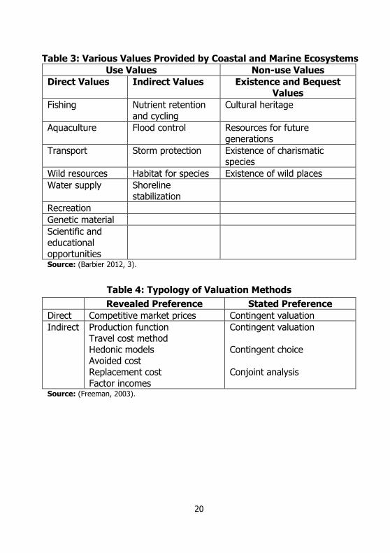
In the light of the discussion in this paper coastal and marine
ecosystems provide the following benefits as listed in Table 3. The rest of
this paper is arranged as follows: Section briefly recounts the relevant
literature on coastal and marine ecosystems – both theoretical and
empirical contributions. The methodology followed for valuing
recreational services using the Travel Cost method in this paper is
described in Section 3 and the estimates are discussed in Section 4. The
paper concludes with a short discussion in Section 5.
LITERATURE SURVEY
It is one thing to identify the ecosystem service and know its
magnitude— how much the physical flows and stocks are, but quite a
different proposition to figure out how much of its use would be
sustainable. An exercise in valuation is helpful in arriving at these crucial
decisions. But this is easier said than done. The problem arises on two
counts – a) many natural resources are not directly traded in the market
and therefore do not have a direct market price, and (b) when the
market price does exist, it may not reflect the true social value.
There are a number of techniques in the economist’s tool-box
that allow us to value natural resources but these are classified into two
broad categories – the revealed preference and the stated preference
methods. The revealed preference methods infer values from actual
3
observed behaviour and, therefore, are least controversial when
observation and analysis is based on them. Stated preference methods
place hypothetical but realistic situations to the respondent (consumer or
producer) and infer values based on their responses.
If there are existing market prices then direct valuation can be
done as in the case of fisheries. However, on other occasions proxy
measures using indirect (non-market) methods come in handy. The
production function approaches, the hedonic models, travel cost methods
are the most popular (see Table 4).
There are various occasions when revealed preference is not
feasible – specifically when markets don’t exist which is very often the
case when we think of environmental services. Then one does not have
any option but to rely on stated preference methods. In the early years,
stated preference methods were treated with suspicion. This was
primarily because they were done with poor techniques, and the values
generated differed widely from other revealed preference methods.
However, following the National Oceanic and Atmospheric Administration
(NOAA) guidelines of “good practice”, norms in conducting stated
preference valuation have been established (Arrow et al. 1993).
Increasingly, stated preference values seem to be in the near vicinity of
comparable revealed preference values (Carson 2012).
The stated preference methods have come to be synonymous
with Contingent Valuation (CVM) among economists. Apart from the
CVMs, contingent choice models and Conjoint Analysis Method are also
used for ranking of choices (Farber and Griner, 2000).
Often, in the absence of or to compare the estimates from the
methods described above, a widely used method is the value (or benefit)
transfer method. Values are taken from previously done studies from
4
different geographical zones and contextualized to generate values for a
local area.
The Total Economic Value (TEV) framework is widely accepted
for resource valuation (Krutilla and Fisher 1975; Pearce and Turner
1990). It anticipates that ecosystems have multiple “use” (direct and
indirect) and “non-use” benefits. To get a comprehensive estimate of the
value of an ecosystem, the different benefits could be added up.
Given the huge interest in valuation studies and the manner in
which some are conducted, there have been concerns that researchers
need to be careful in their estimation techniques. One common error that
arises is of double counting. When following the MA (MA 2005)
classification, ecosystem values are summed across different categories
– supporting, regulating, provisioning and cultural. This could lead to
over-valuation due to double counting. Caution also needs to be
exercised to distinguish between intermediate services and final services.
Valuation should focus on benefits from final services (Boyd and Banzhaf
2007; B. Fisher, Bateman, and Turner 2011). For example, in the coastal
and marine systems, water regulation, mangrove generation and soil
formation are intermediate services whereas storm protection, clean
water provision are final services that accord benefits like protection of
property and life, recreation, greater fish catch, etc. (Brendan Fisher,
Turner, and Morling 2009).
Macro Estimates
It is not possible here to summarise or even attempt a review of the
literature, but it is worth mentioning that most of the studies are local
and geographically specific. While this is most practical and efficient,
macro level assessments assume importance especially when one is
dealing with national level policies and global interventions for
sustainable use of resources. The attempts at Green Accounting are an
attempt in this direction. And yet National or international level studies
5
are still rare. An early attempt at valuing the global ecosystem service
flows, which were not accounted for in the regular national income
accounts, was about US$ 33 trillion per year (when the global GDP was
US$ 18 trillion in 1997 at 1994 US$ US prices) (Costanza et al. 1997).
Coastal and marine ecosystems which formed a part of this was
estimated to be US$ 20.9 trillion per year (excluding wetlands). In 2014,
the annual flow of ecosystem services was estimated to be US$145
trillion per year (in comparison to global GDP of US$ 75.2 trillion per year
in 2011 at 2007 US$ prices) and coastal and marine ecosystems
contributed US$ 60.5 trillion per year (Costanza et al. 2014).
Indian Assessments
The literature on valuation of ecosystem services in India is rather thin
(Mukhopadhyay and Shyamsundar 2015; Parikh et al. 2012). The most
widely used searchable compilation of peer reviewed valuation studies is
the Ecosystem Services Valuation Database (ESVD) (van der Ploeg and
de Groot 2010). Of the 1310 listed studies here only 62 were from South
Asia and 24 from India. If one were to focus only on the coastal and
marine systems, we would find 518 studies listed under the following
biomes ecosystems: coastal wetlands, coral reefs, coastal and marine,
which cover the following ecosystems: coastal and marine, open oceans,
swamps/marshes, tidal marshes, multiple ecosystems, mangroves, coral
reefs, continental shelf sea, estuaries, seagrass and algae beds, shores
and salt water wetlands. India accounts for only 9 of the listed studies
(Yadava, Mukhopadhyay, and Bhatt 2015).
There are some studies available outside the TEEB database.
One such widely cited study concluded that mangroves reduced deaths
by 54% from wind and storm damages during the super-cyclone of 1999
in Orissa (Das and Vincent 2009). A valuation exercise of Ashtamudi
Estuary in Kerala, a Ramsar site by Anoop and Suryaprakash (2008)
estimated the Option Value of the estuary to be Rs. 3.88 million and the
present value of the estuary to be Rs. 87.1 million. The use values (direct
6
– fishery, husk retting, inland navigation and recreation; and indirect
benefits – carbon sequestration and shrimp larvae protection) emanating
from the same estuary was estimated to yield net benefits amounting to
Rs. 1924 million (Anoop et al. 2008). The Coral Reefs of Gulf of Kachchh
was estimated to provide ecosystem benefits worth Rs. 2200.24 million
(2007 prices) at the rate of Rs. 7.95 million per km2 from five services
(fisheries, recreation, biodiversity and protection against salinity ingress
and erosion) (Dixit et al. 2010, 2012). The recreational value of Indian
Sunderbans, a UNESCO World Heritage and a Ramsar site was estimated
by (Guha and Ghosh 2011) to be approximately to US$ 377,000 (in the
year 2006).
There are however, no national level estimates available in India
for coastal and marine ecosystems. And therefore any attempt to arrive
at some estimate is an important pursuit. A consortium of researchers
from the Goa University, Madras School of Economics and National
Centre for Sustainable Coastal Management, are attempting to provide a
consolidated estimate of coastal and marine ecosystem services in India.
As part of this exercise, this paper proposes to estimate the benefits
derived from recreation from coastal and marine ecosystem services.
METHODOLOGY
The most widely used method for estimating recreational benefits is the
travel cost method (TC). It relies on estimating a demand curve for
visitation with respect to cost of travel. This helps in calculating the
welfare value per visitor or household (depending on the unit of
analysis). The utility function is integrated between the present price
faced by the household for the complementary good and the choke price,
i.e., the price at which the quantity demanded goes down to zero. The
travel expenditure places a floor price to what the consumer is willing to
pay for recreation.
7
A popular TC method is the Individual Travel Cost method
(ITCM). For this method to work well data collection is done at the
individual visitor level and relies on the visitor to make multiple visits to
the same site in a specified time. The demand curve then is derived by
correlating the number of visits (visitation rate) with the cost of travel to
the site. If well implemented this can generate a reliable demand curve
from which predictions on willingness to pay for change in quality of the
site can be predicted.
Even though this method is more accurate, it is very data
intensive. A less data demanding alternate method is the Zonal Travel
Cost Method (ZTCM) which instead of asking how many times an
individual visitor comes to a site, relies on how many visitors come from
a region (also called a zone). The visitation rate from a region is
estimated by dividing the number of visitors by the population of the
originating region/zone. The visitation rate is expected to be dependent
on the cost of travel from the region among other characteristics of that
region. The empirical estimation of the demand relies on a Trip
Generating Function (TGF) and the number of data points is determined
(and equal to) the number of zones.
The issues that require consideration are:
(a) A suitable functional form for the TGF. Linear and log-linear
forms are most oft used.
(b) Optimum number of zones: In our study the optimum number of
zones was defined by the number of states for which state of
origin data was available.
(c) Issue of multipoint tourists: The issue of multi-point tourists is a
vexing problem in the TCM and no satisfactory solution exists in
the literature. However, in our study we ourselves are dealing
with a collection of multiple point visits though restricted to the
coast. Effectively it reduces visits to two points – coast and non-
coast. We have assumed that the amount of time and money
8
spent by a visitor in the coast is directly related to proportion of
the population in the district.
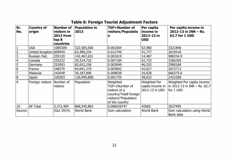
(d) Foreign tourists: In order to incorporate foreign travelers we
picked data from the 8 most popular origins of foreign visitors
(apart from Bangladesh who are largely not recreational visitors).
We treated the foreign visitors as multi-point visitors in India so
we did not include the cost of their international travel. However,
we included cost of domestic travel from the most distant state.
In each state’s estimate it was the state of origin with the highest
distance that was used to compute their cost on travel. Since
separate data is not available for country of origin in each state
we clubbed all foreign tourists into one set and calculated their
weighted TGF and income for the country. In order to further
calibrate for over estimation we used half this value as the per
capita income of an average foreign visitor as a large proportion
of visitors come from countries that do not have as high a per
capita income as USA or UK (like Spain or Italy). Thereafter the
same calculation steps were followed as was done for domestic
tourists.
(e) Zero zonal visitation rate: This was avoided by dropping zones
from where there was no visitation or clubbing states to create
acceptable zones.
(f) Uneven distributional variance (heteroskedasticity) in zonal data:
In order to control for hetroskedasticity one could use robust
standard errors to get corrected parametric values. However
since in this paper we do not attempt any regression we leave
this for a later occasion. This paper has a much narrower
objective.
There have been some applications of the ZTCM in parts of India,
namely, the Keoladeo National Park (India) (Chopra, 2004) and the
Sunderbans (Guha and Ghosh, 2013). However, there is no country wide
9
estimate of the recreation value of coastal and marine eco-systems and
this study therefore is the first such attempt.
The Travel Cost Method was introduced by Hotelling (1947). It
plays on the idea that the amount of money a visitor pays for recreation
is a floor value of the recreational value for the site. Like all other normal
goods, visitation is expected to be inversely related to the cost of travel.
The recreational demand can be estimated using travel cost after
adjusting for other socio-economic factors. If travel cost increases with
distance, then the distance from different zones would determine the
visitation to the site. In the absence of further information, it is implicitly
assumed visitors across regions have similar tastes and preferences.
Model of Zonal Travel Cost Method
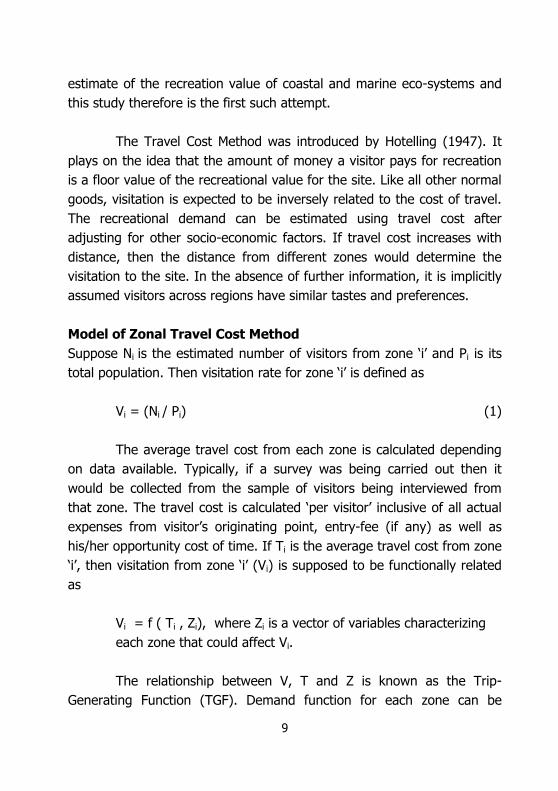
Suppose Ni is the estimated number of visitors from zone ‘i’ and Pi is its
total population. Then visitation rate for zone ‘i’ is defined as
Vi = (Ni / Pi) (1)
The average travel cost from each zone is calculated depending
on data available. Typically, if a survey was being carried out then it
would be collected from the sample of visitors being interviewed from
that zone. The travel cost is calculated ‘per visitor’ inclusive of all actual
expenses from visitor’s originating point, entry-fee (if any) as well as
his/her opportunity cost of time. If Ti is the average travel cost from zone
‘i’, then visitation from zone ‘i’ (Vi) is supposed to be functionally related
as
Vi = f ( Ti , Zi), where Zi is a vector of variables characterizing
each zone that could affect Vi.
The relationship between V, T and Z is known as the Trip-
Generating Function (TGF). Demand function for each zone can be
10
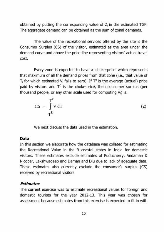
obtained by putting the corresponding value of Zi in the estimated TGF.
The aggregate demand can be obtained as the sum of zonal demands.
The value of the recreational services offered by the site is the
Consumer Surplus (CS) of the visitor, estimated as the area under the
demand curve and above the price-line representing visitors’ actual travel
cost.
Every zone is expected to have a ‘choke-price’ which represents
that maximum of all the demand prices from that zone (i.e., that value of
Ti for which estimated Vi falls to zero). If T0 is the average (actual) price
paid by visitors and TC is the choke-price, then consumer surplus (per
thousand people, or any other scale used for computing Vi) is:
cT
0T
dT V CS (2)
We next discuss the data used in the estimation.
Data
In this section we elaborate how the database was collated for estimating
the Recreational Value in the 9 coastal states in India for domestic
visitors. These estimates exclude estimates of Puducherry, Andaman &
Nicobar, Lakshwadeep and Daman and Diu due to lack of adequate data.
These estimates also currently exclude the consumer’s surplus (CS)
received by recreational visitors.
Estimates
The current exercise was to estimate recreational values for foreign and
domestic tourists for the year 2012-13. This year was chosen for
assessment because estimates from this exercise is expected to fit in with
11
and be comparable with benefit estimates from other ecosystem services
being done by colleagues at MSE and the NCSCM.
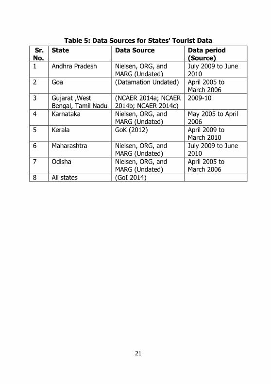
Even though tourism is well developed service sector, secondary
data availability in the tourism sector is still sparse for our kind of
analysis. Therefore we have had to rely on numerous sources for putting
these variables in a usable format. There were primary surveys
conducted as part of a larger exercise across many Indian states by the
Ministry of Tourism, Government of India. These however, do not cover
all the coastal states and it was a one shot exercise (for details see Table
5). As the data for different states was for different years we had to
extrapolate for the relevant year 2012-13. The details of methods used
are described in Table 7.
In order to estimate the actual travel cost three different broad
categories of expenses were computed – expense on travel, expense on
accommodation and food, and opportunity cost of spending time on
recreation. These three were then added to arrive at the actual total cost
of travel from different zones to a particular destination. Finally, these
were totaled for all the 9 states to arrive at the aggregate value for the
country.
(a) Estimation of travel expense: This value was obtained by
multiplying the distance from the state of origin to the most
visited recreation site of the host state by the cost per unit
(kilometer) travelled. The per kilometer rate of travel which was
assumed to be Rs. 8/km -- the reason for taking Rs. 8 was that
the government approved rate of travel is Rs. 16. But for long
distance this was considered very high. So we decided to use half
that value for estimating travel expense to balance of people
travelling by different modes of travel to the host state.
12
(b) Expense on Accommodation and food, etc.: Data is
available from different sources on the number of days/nights
overnight visitors spend in the host state and how much on
average a visitor spends there. While for three states (Karnataka,
Andhra Pradesh and Maharashtra) data is available for 2009-10,
for two states (Goa and Odisha) it is available for 2005-6 from
surveys. We multiplied this figure (which is a common number
for all originating states as there is no state-wise data available)
with the per capita income of the origin state to adjust for
differences in expenditure patterns.
(c) Opportunity cost: One of the continuing debates in empirical
estimation has been the valuation of travel time – the
opportunity cost of travel, much after Clawson and Knetsch
(1966) raised this half a century ago. A number of approaches
have been adopted in the literature to deal with this issue which
fall under two broad categories: (a) exclude opportunity cost,
and (b) include opportunity cost as a fraction of the respondent’s
wage rate (some have used 100% of forgone wages).
We have used the per capita income for 2012-13 for each
originating state and multiplied it by the number of visitors to the
host state. Since there is a wide range of incomes earned within
each state, the fractioning of incomes is likely to have been
achieved by taking the average of income of the state.
Each of the above figures was multiplied by proportion of
population in coastal districts (except for Goa where this was done at the
taluka level). The population of coastal districts was divided by the
population of the state to obtain this number. It was assumed that the
distribution of the recreational visitors to coastal states would follow a
pattern exhibited by the distribution of population of the state. This was
13
further multiplied by the percentage of recreational visitors wherever this
data was available.
Discussion and Conclusion
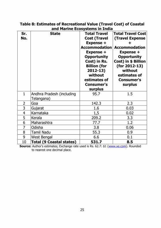
The estimates for each state are presented in Table 8 below. These are
floor level values as they do not include the estimates of consumer’s
surplus. Our estimates suggest that the extent of ecosystem services on
account of recreation is about Rs. 531.8 billion in 2012-13 prices. Since
we do not have any other study in India against which to benchmark our
estimates we are unable to say whether our estimates are high or low at
this point. In 2012-13, the contribution from “Hotels and Restaurants” in
India to GDP was Rs. 1360.8 billion when India’s GDP was estimated at
Rs. 93888.76 billion.
Interestingly, Kerala topped the recreational services followed by
Goa – both being much smaller states than their neighbours both on the
eastern and western coasts. However, both these states have had the
advantage of being popular and long stay tourist destinations with the
bulk of the tourism concentrated along the coast. These estimates are
critically dependent on the quality of the data collected from secondary
surveys. The authors hope that these estimates will provide a way and
encourage further research on estimation of macro estimates of
ecosystem services. It is expected that the final value of these services
will be higher than what this estimate suggests as it constitutes only
what the consumers (recreational visitors) spent in their travel by way of
cost of travel, accommodation and income forgone (opportunity cost).
These estimates therefore should be treated as a partial analysis and a
floor value.
14
REFERENCE
Anoop, P., and S. Suryaprakash (2008), “Estimating the Option Value of Ashtamudi Estuary in South India: A Contingent Valuation Approach”, Presented at the 12th Congress of the European Association of Agricultural Economists, Ghent, Belgium, August 26. http://ageconsearch.umn.edu/bitstream/43607/2/066.pdf.
Anoop, P., S. Suryaprakash, K.B. Umesh, and T.S. Amjath Babu (2008), “Economic Valuation of Use Benefits of Ashtamudi Estuary in South India”, In Proceedings of the Taal 2007: The 12th World Lake Conference, edited by M. Sengupta and R. Dalwani, 1822–26. http://moef.nic.in/modules/recent-initiatives/nlcp/Indian% 20Case%20Studies/Q-7.pdf.
Arrow, K., R. Solow, Paul R. Portney, E.E. Leamer, R. Radner, and H. Schuman (1993), Report of the NOAA Panel on Contingent Valuation. National Oceanic and Atmospheric Administration. www.economia.unimib.it/DATA/moduli/7_6067/.../noaa%20report.pdf.
Barbier, E. B. (2012), “Progress and Challenges in Valuing Coastal and Marine Ecosystem Services”, Review of Environmental Economics and Policy 6 (1): 1–19. doi:10.1093/reep/rer017.
Boyd, J., and S. Banzhaf (2007), “What Are Ecosystem Services?”, Ecological Economics 63: 616–26.
Carson, Richard T. (2012), “Contingent Valuation: A Practical Alternative When Prices Aren’t Available”, Journal of Economic Perspectives 26 (4): 27–42. doi:10.1257/jep.26.4.27.
Clawson, M, and J Knetsch (1966), “Economics of Outdoor Recreation”, Washington, D.C.: Resources For Future.
Costanza, R., R. d’Arge, R. de Groot, Stephen C. Farber, M. Grasso, B. Hannon, S. Naeem, et. al. (1997), “The Value of the World’s Ecosystem Services and Natural Capital”, Nature 387: 253–60.
15
Costanza, Robert, Rudolf de Groot, Paul Sutton, Sander van der Ploeg, Sharolyn J. Anderson, Ida Kubiszewski, Stephen Farber, and R. Kerry Turner (2014), “Changes in the Global Value of Ecosystem Services”, Global Environmental Change 26 (May): 152–58. doi:10.1016/j.gloenvcha.2014.04.002.
Das, S., and J. R. Vincent (2009), “Mangroves Protected Villages and Reduced Death Toll during Indian Super Cyclone”, Proceedings of the National Academy of Sciences 106 (18): 7357–60. doi:10.1073/pnas.0810440106.
Datamation, Undated, (2006), “Collection of Domestic Tourism Statistics For the State of Goa: Final Report (April 2005 to March 2006)”, New Delhi: Ministry of Tourism, Government of India. http://tourism.gov.in/CMSPagePicture/file/marketresearch/statisticalsurveys/03%20goa.pdf.
Dixit, Arun M., Lalit Kumar, Pushpam Kumar, and Kinjal Pathak (2012), “Valuing the Services of Coral Reef Systems for Sustainable Coastal Management: A Case Study of the Gulf of Kachchh, India”, In Valuation of Regulating Services of Ecosystems : Methodology and Applications, edited by Pushpam Kumar and Michael D Wood, 175–98. London: Routledge.
Dixit, Arun M., Lalit Kumar, Pushpam Kumar, Kinjal Pathak, and M.I. Patel (2010), “Economic Value of Coral Reef Systems in Gulf of Kachchh”, Final Report, World Bank Aided Integrated Coastal Zone Management (ICZM) Project, Gandhinagar: Gujarat Ecology Commission.
Farber, Stephen, and Brian Griner (2000), “Using Conjoint Analysis To Value Ecosystem Change †”, Environmental Science and Technology 34 (8): 1407–12. doi:10.1021/es990727r.
Fisher, B., Ian Bateman, and R. Kerry Turner (2011), “Valuing Ecosystem Services: Benefits, Values, Space and Time”, No. 3. Na: United Nations Environment Programme.
16
Fisher, Brendan, R. Kerry Turner, and Paul Morling (2009), “Defining and Classifying Ecosystem Services for Decision Making”, Ecological Economics 68 (3): 643–53. doi:10.1016/j.ecolecon.2008.09.014.
Freeman, A. Myrick (2003), The Measurement of Environmental and Resource Values : Theory and Methods. Washington, DC: Resources for the Future.
GoI (2014), “India Tourism Statistics at a Glance 2013”, New Delhi: Ministry of Tourism, Government of India. http://tourism.gov.in/writereaddata/CMSPagePicture/file/marketresearch/Incredible%20India%20final%2021-7-2014%20english.pdf.
——— (2015), “Agricultural Statistics at a Glance 2014”, New Delhi: Ministry of Agriculture Department of Agriculture and Cooperation Directorate of Economics and Statistics.
GoK (2012), “Kerala Tourism Statistics 2010”, Thiruvananthapuram: Department of Tourism, Government of Kerala. https://www.keralatourism.org/tourist-statistics-2010-new.pdf.
Guha, Indrila, and Santadas Ghosh (2011), “Valuing the Land of Tigers: What Indian Visitors Reveal”, In Environmental Valuation in South Asia, edited by A. K. Enamul Haque, M. N Murty, and Priya Shyamsundar, 232–55. New Delhi: Cambridge University Press. http://dx.doi.org/10.1017/CBO9780511843938.011.
Krutilla, John V, and Anthony C Fisher (1975), The Economics of Natural Environments : Studies in the Valuation of Commodity and Amenity Resources. Washington, D.C.; Baltimore, Md.: Resources for the Future : Distributed worldwide by the Johns Hopkins University Press.
MA (2005), Millennium Ecosystem Assessment, Washington, DC: Island Press.
Mukhopadhyay, Pranab, and Priya Shyamsundar (2015), “Ecosystem Services – An Agenda for Research in South Asia”, 88–15, Policy
17
Brief, Kathmandu: South Asian Network for Development and Environmental Economics.
NCAER (2014a), “Regional Tourism Satellite Account Gujrat, 2009-10”, New Delhi: Ministry of Tourism, Government of India.
——— (2014b), “Regional Tourism Satellite Account Tamil Nadu, 2009-10.” New Delhi: Ministry of Tourism, Government of India.
——— (2014c), “Regional Tourism Satellite Account West Bengal, 2009-10”, New Delhi: Ministry of Tourism, Government of India.
Nielsen, A.C., ORG, and MARG. Undated, “Collection of Domestic Tourism Statistics for the State of Karnataka”, New Delhi: Ministry of Tourism, Government of India. http://tourism.gov.in/CMSPagePicture/file/marketresearch/statisticalsurveys/011%20karnataka.pdf.
——— Undated, “Collection of Domestic Tourism Statistics For the State of Orissa”, New Delhi: Ministry of Tourism, Government of India. http://tourism.gov.in/CMSPagePicture/file/marketresearch/statisticalsurveys/012%200rissa.pdf.
——— Undated, “Tourism Survey for Andhra Pradesh”, Ministry of Tourism, Government of India. http://tourism.gov.in/writereaddata/CMSPagePicture/file/marketresearch/statisticalsurveys/AP.pdf.
——— Undated, “Tourism Survey for State of Maharashtra”, New Delhi: Ministry of Tourism, Government of India. http://tourism.gov.in/writereaddata/CMSPagePicture/file/marketresearch/statisticalsurveys/Maharashtra.pdf.
Parikh, K., N.H. Ravindranath, I.K. Murthy, S. Mehra, R. Kumar, EJ James, E. Vivekanandan, and Pranab Mukhopadhyay (2012), “The Economics of Ecosystems and Biodiversity - India: Initial Assessment and Scoping Report”, Working Document. New Delhi: Ministry of Environment and Forests, Government of India.
18
Pearce, David W, and R. Kerry Turner (1990), Economics of Natural Resources and the Environment, Baltimore: Johns Hopkins University Press.
UNEP-WCMC (2011), “Marine and Coastal Ecosystem Services: Valuation Methods and Their Application”, Biodiversity Series No. 33. UNEP-WCMC. www.unep-wcmc.org.
van der Ploeg, S., and R.S. de Groot (2010), “The TEEB Valuation Database – a Searchable Database of 1310 Estimates of Monetary Values of Ecosystem Services”, Wageningen, The Netherlands.: Foundation for Sustainable Development.
Yadava, Yugraj, Pranab Mukhopadhyay, and J.R. Bhatt (2015), “Incentives for Sustainable Management of Biodiversity and Ecosystem Services- TEEB India Initiative: Study Report- Coastal and Marine Ecosystem”, New Delhi: MOEFCC and GIZ.
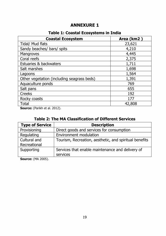
19
ANNEXURE 1
Table 1: Coastal Ecosystems in India
Coastal Ecosystem Area (km2 )
Tidal/ Mud flats 23,621
Sandy beaches/ bars/ spits 4,210
Mangroves 4,445
Coral reefs 2,375
Estuaries & backwaters 1,711
Salt marshes 1,698
Lagoons 1,564
Other vegetation (including seagrass beds) 1,391
Aquaculture ponds 769
Salt pans 655
Creeks 192
Rocky coasts 177
Total 42,808 Source: (Parikh et al. 2012).
Table 2: The MA Classification of Different Services
Type of Service Description
Provisioning Direct goods and services for consumption
Regulating Environment modulation
Cultural and Recreational
Tourism, Recreation, aesthetic, and spiritual benefits
Supporting Services that enable maintenance and delivery of services
Source: (MA 2005).
20
Table 3: Various Values Provided by Coastal and Marine Ecosystems
Use Values Non-use Values
Direct Values Indirect Values Existence and Bequest Values
Fishing Nutrient retention and cycling
Cultural heritage
Aquaculture Flood control Resources for future generations
Transport Storm protection Existence of charismatic species
Wild resources Habitat for species Existence of wild places
Water supply Shoreline stabilization
Recreation
Genetic material
Scientific and educational opportunities
Source: (Barbier 2012, 3).
Table 4: Typology of Valuation Methods
Revealed Preference Stated Preference
Direct Competitive market prices Contingent valuation
Indirect Production function Travel cost method Hedonic models Avoided cost Replacement cost Factor incomes
Contingent valuation Contingent choice Conjoint analysis
Source: (Freeman, 2003).
21
Table 5: Data Sources for States' Tourist Data
Sr. No.
State Data Source Data period (Source)
1 Andhra Pradesh Nielsen, ORG, and MARG (Undated)
July 2009 to June 2010
2 Goa (Datamation Undated) April 2005 to March 2006
3 Gujarat ,West Bengal, Tamil Nadu
(NCAER 2014a; NCAER 2014b; NCAER 2014c)
2009-10
4 Karnataka Nielsen, ORG, and MARG (Undated)
May 2005 to April 2006
5 Kerala GoK (2012) April 2009 to March 2010
6 Maharashtra Nielsen, ORG, and MARG (Undated)
July 2009 to June 2010
7 Odisha Nielsen, ORG, and MARG (Undated)
April 2005 to March 2006
8 All states (GoI 2014)
22
Table 6: Foreign Tourist Adjustment Factors
Sr. No.
Country of origin
Number of visitors in 2013 from top 8 countries
Population in 2013
TGF=Number of visitors/Population
Per capita income in 2012-13 in USD
Per capita income in 2012-13 in INR – Rs. 62.7 for 1 USD
1 USA 1085309 322,583,006 0.003364 52,980 3321846
2 United Kingdom 809444 63,489,234 0.012749 41,777 2619418
3 Russian Fed. 259120 142,467,651 0.001819 14,487 908334.9
4 Canada 255222 35,524,732 0.007184 52,733 3306359
5 Germany 252003 82,652,256 0.003049 46,255 2900189
6 France 248379 64,641,279 0.003842 42,627 2672713
7 Malaysia 242649 30,187,896 0.008038 10,628 666375.6
8 Japan 220283 126,999,808 0.001735 38,633 2422289
9 Foreign visitors Number of visitors
Population Weighted TGF=(Number of visitors of a country/Totall foreign visitors)*Population of the country
Weighted Per capita income in 2012-13 in USD
Weighted Per capita income in 2012-13 in INR – Rs. 62.7 for 1 USD
10 All Total 3,372,409 868,545,862 0.006028747 42065 2637495
Source: (GoI 2014) World Bank Own calculation World Bank Own calculation using World Bank data
23
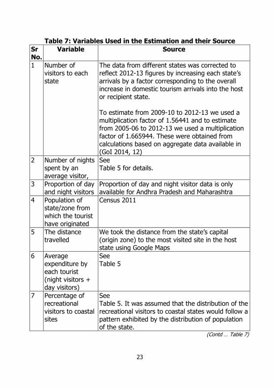
Table 7: Variables Used in the Estimation and their Source
Sr No.
Variable Source
1 Number of visitors to each state
The data from different states was corrected to reflect 2012-13 figures by increasing each state’s arrivals by a factor corresponding to the overall increase in domestic tourism arrivals into the host or recipient state. To estimate from 2009-10 to 2012-13 we used a multiplication factor of 1.56441 and to estimate from 2005-06 to 2012-13 we used a multiplication factor of 1.665944. These were obtained from calculations based on aggregate data available in (GoI 2014, 12)
2 Number of nights spent by an average visitor,
See Table 5 for details.
3 Proportion of day and night visitors
Proportion of day and night visitor data is only available for Andhra Pradesh and Maharashtra
4 Population of state/zone from which the tourist have originated
Census 2011
5 The distance travelled
We took the distance from the state’s capital (origin zone) to the most visited site in the host state using Google Maps
6 Average expenditure by each tourist (night visitors + day visitors)
See Table 5
7 Percentage of recreational visitors to coastal sites
See Table 5. It was assumed that the distribution of the recreational visitors to coastal states would follow a pattern exhibited by the distribution of population of the state.
(Contd … Table 7)
24
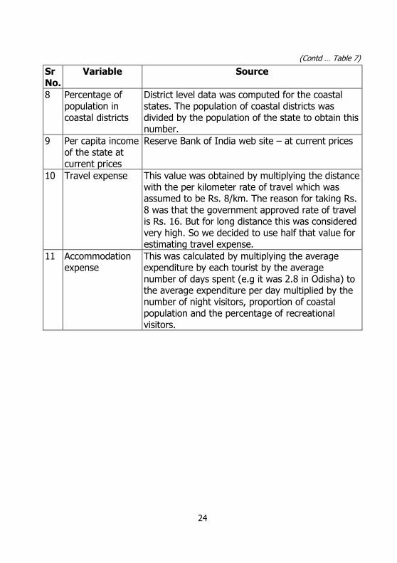
(Contd … Table 7)
Sr No.
Variable Source
8 Percentage of population in coastal districts
District level data was computed for the coastal states. The population of coastal districts was divided by the population of the state to obtain this number.
9 Per capita income of the state at current prices
Reserve Bank of India web site – at current prices
10 Travel expense This value was obtained by multiplying the distance with the per kilometer rate of travel which was assumed to be Rs. 8/km. The reason for taking Rs. 8 was that the government approved rate of travel is Rs. 16. But for long distance this was considered very high. So we decided to use half that value for estimating travel expense.
11 Accommodation expense
This was calculated by multiplying the average expenditure by each tourist by the average number of days spent (e.g it was 2.8 in Odisha) to the average expenditure per day multiplied by the number of night visitors, proportion of coastal population and the percentage of recreational visitors.
25
Table 8: Estimates of Recreational Value (Travel Cost) of Coastal and Marine Ecosystems in India
Sr. No.
State Total Travel Cost (Travel Expense +
Accommodation Expense +
Opportunity Cost) in Rs. Billion (for 2012-13) without
estimates of Consumer's
surplus
Total Travel Cost (Travel Expense
+ Accommodation
Expense + Opportunity
Cost) in $ Billion (for 2012-13)
without estimates of Consumer's
surplus
1 Andhra Pradesh (including Telangana)
95.7 1.5
2 Goa 142.3 2.3
3 Gujarat 1.6 0.03
4 Karnataka 1,5 0.02
5 Kerala 209.2 3.3
6 Maharashtra 77.7 1.2
7 Odisha 3.8 0.06
8 Tamil Nadu 55.3 0.9
9 West Bengal 6.6 0.1
10 Total (9 Coastal states) 531.7 8.5 Source: Author’s estimates; Exchange rate used is Rs. 62.7: $1 (www.xe.com). Rounded
to nearest one decimal place.
MSE Monographs
* Monograph 22/2012A Macro-Fiscal Modeling Framework for forecasting and Policy SimulationsD.K. Srivastava, K. R. Shanmugam and C.Bhujanga Rao
* Monograph 23/2012Green Economy – Indian PerspectiveK.S. Kavikumar, Ramprasad Sengupta, Maria Saleth, K.R.Ashok and R.Balasubramanian
* Monograph 24/2013Estimation and Forecast of Wood Demand and Supply in TamilanduK.S. Kavi Kumar, Brinda Viswanathan and Zareena Begum I
* Monograph 25/2013Enumeration of Crafts Persons in IndiaBrinda Viswanathan
* Monograph 26/2013Medical Tourism in India: Progress, Opportunities and ChallengesK.R.Shanmugam
* Monograph 27/2014Appraisal of Priority Sector Lending by Commercial Banks in IndiaC. Bhujanga Rao
* Monograph 28/2014Fiscal Instruments for Climate Friendly Industrial Development in Tamil NaduD.K. Srivastava, K.R. Shanmugam, K.S. Kavi Kumar and Madhuri Saripalle
* Monograph 29/2014Prevalence of Undernutrition and Evidence on Interventions: Challenges for IndiaBrinda Viswanathan.
* Monograph 30/2014Counting The Poor: Measurement And Other IssuesC. Rangarajan and S. Mahendra Dev
* Monograph 31/2015
Technology and Economy for National Development: Technology Leads to Nonlinear Growth
Dr. A. P. J. Abdul Kalam, Former President of India
* Monograph 32/2015
India and the International Financial System
Raghuram Rajan
* Mongraph 33/2015
Fourteenth Finance Commission: Continuity, Change and Way Forward
Y.V. Reddy
Pranab Mukhopadhyay Vanessa da Costa
MADRAS SCHOOL OF ECONOMICSGandhi Mandapam Road
Chennai 600 025 India
September 2015
RECREATIONAL VALUE OF COASTAL AND MARINE ECOSYSTEMS IN INDIA:
A PARTIAL ESTIMATE
MSE Working Papers
Recent Issues
* Working Paper 112/2015Health Shocks and Short-Term Consumption GrowthSowmya Dhanaraj
* Working Paper 113/2015Efficiency in Elementary Education in Urban India: An Exploratory Analysis Using DeaBrijesh C. Purohit
* Working Paper 114/2015Price Rigidity, Inflation And The Distribution Of Relative Price ChangesSartaj Rasool Rather, S. Raja Sethu Durai and M. Ramachandran
* Working Paper 115/2015Money and Inflation: Evidence from P-Star ModelSunil Paul, Sartaj Rasool Rather and M. Ramachandran
* Working Paper 116/2015Determinants of Energy and Co2 Emission Intensities: A Study of Manufacturing Firms in IndiaSantosh K. Sahu and Deepanjali Mehta
* Working Paper 117/2015Impact of Water and Sanitation on Selected Water Borne Diseases in IndiaBrijesh C. Purohit
* Working Paper 118/2015Health Shocks and Inter-Generational Transmission of InequalitySowmya Dhanaraj
* Working Paper 119/2015Productivity, Energy Intensity and Output: A Unit Level Analysis of the Indian Manufacturing SectorSantosh K. Sahu and Himani Sharma
* Working Paper 120/2015Health Shocks and Coping Strategies: State Health Insurance Scheme of Andhra Pradesh, IndiaSowmya Dhanaraj
* Working Paper 121/2015Efficiency in Education Sector: A Case of Rajasthan State (India)Brijesh C Purohit
* Working Paper 122/2015Mergers and Acquisitions in the Indian Pharmaceutical SectorSantosh Kumar Sahu and Nitika Agarwal
* Working Paper 123/2015Analyzing the Water Footprint of Indian Dairy IndustryZareena B. Irfan and Mohana Mondal
* Working papers are downloadable from MSE website http://www.mse.ac.in
$ Restricted circulation
WORKING PAPER 124/2015