MSc Thesis Chair Group Business Economics Agricultural ...

Wageningen University - Department of Social Sciences MSc Thesis Chair Group Business Economics

Agricultural Commodity prices & the Stock Market ‘Testing for price relationships between agricultural

commodities and food corporations’ shares by using

statistical analysis’

May 2015

Management Economics and Consumer Studies

Business Economics

Arjan van der Meijden

Prof.dr.ir. AGJM (Alfons) Oude Lansink

MSc. Tsion Assefa BEC-80433

2

Agricultural Commodity Prices & the Stock Market

‘Testing for price relationships between agricultural commodities and food corporations’ shares by using statistical analysis’

Arjan van der Meijden

3

Abstract The value of a firm can be calculated by dividing the free cash flow to the firm by the discount rate. Share prices are a representation of this value. The volatility of commodity prices has been remarkable over the past decade and due to this increased volatility, it has become harder for firms in the food- and agribusiness to ensure continuity in their cash flows. The (dis)ability of a corporation to create continuity in its cash flows, due to its dependency on commodity prices, can therefore result in an increased volatility in stock prices as well. The relationship between volatility in commodity prices and the effect on stock prices is however not exactly clear yet. The objective of this thesis is to further investigate this relation. The main question that needs to be answered is: What is the relation between agricultural commodity prices and a food corporations’ stock price? To answer this question, the following sub questions have to be addressed as well: What factors determine a corporation’s share price in theory? & What is the correlation between stock prices and commodity prices? It was found that in theory, share prices are determined by dividing the expected future dividends by the discount rate; P0=∑Divt/(1+Rt)

t. Furthermore, according to the current literature, factors that can influence the

market value of shares are: the financial structure of the firm, the media, investor sentiment, customer satisfaction, macro-economic factors and commodity prices. Econometric analysis has been used to answer the second sub question. The closing prices of different commodities and stocks have been gathered over a period of time. With this data, an ordinary least squares regression has been executed, where the stock prices were the dependent variables (y) and the commodity prices the explanatory variables (x). The results of the econometric analysis suggest that the effect of commodity price volatility on a food corporations share price is small, provided that the firms have a solid risk management strategy for the procurement of raw material. A successful strategy can ensure continuity in cash flows and thereby lead to more stability in share prices.

4

Index 1. Introduction ........................................................................................................................ 5

1.1 Problem statement ....................................................................................................... 5

1.2 Objectives .................................................................................................................... 6

1.3 Reading guide .............................................................................................................. 6

2. Empirical Framework ......................................................................................................... 7

2.1 Share price valuation ................................................................................................... 7

2.2 Factors influencing share prices .................................................................................. 8

2.2.1 Firm specific factors ............................................................................................. 8

2.2.2 The media and investor sentiment ...................................................................... 10

2.2.3 Customer satisfaction ......................................................................................... 10

2.2.4 Macroeconomic factors ...................................................................................... 11

2.2.5 Commodities ...................................................................................................... 12

3. Methodology .................................................................................................................... 13

3.1 Model ......................................................................................................................... 13

3.2 Description of model variables .................................................................................. 14

3.3 Data ............................................................................................................................ 15

4. Results .............................................................................................................................. 16

4.1 Nutreco ...................................................................................................................... 16

4.2 Bongrain .................................................................................................................... 17

4.3 Bunge ......................................................................................................................... 19

4.4 Corbion ...................................................................................................................... 20

4.5 Danone ....................................................................................................................... 21

4.6 Nestlé ......................................................................................................................... 21

4.7 Unilever ..................................................................................................................... 23

5. Discussion ........................................................................................................................ 25

6. Conclusion ........................................................................................................................ 26

References ................................................................................................................................ 27

Appendix A. Search terms Google Scholar & Scopus ....................................................... 29

Appendix B. Tables & Figures ........................................................................................... 30

Table 2. Information Criteria ............................................................................................... 31

Table 3. Reading correlograms ............................................................................................ 32

Correlogram of Bunge’s residuals ........................................................................................ 33

Correlogram of Nestlé’s residuals ........................................................................................ 34

Correlogram of Unilever’s residuals .................................................................................... 35

Appendix C. Risk Management Strategies of the Firms ...................................................... 36

Appendix D. Results of Augmented Dickey Fuller tests ..................................................... 41

5

1. Introduction

1.1 Problem statement One of the ways to calculate the value of a firm is by using the Free Cash Flow to the Firm (FCFF) method. This calculation can be done by dividing the free cash flow to the firm by the discount rate (Hillier et al., 2013). The free cash flow is the cash remaining after all debt and lease obligations have been met (Kaen, 2003). The cash can be returned to the shareholders as dividend payments or reinvested in the firm. Because one of the objectives of corporate governance is to create value for the owners of the corporation (shareholders), managers aim to ensure continuity and growth in the cash flows to the firm (Kaen, 2003). Another way to calculate the firm’s relative value is by using multiples. Most of the times, the numerator of the multiple is the company’s market price (P). For example, the price/earnings ratio (P/E ratio) can be calculated by dividing the company’s market price per share divided by the earnings per share. Variations to this method are the P/EBIT ratio and the P/EBITDA ratio, which use the Earnings Before Interest & Taxes and Earnings Before Interest, Taxes, Depreciation and Amortization respectively (Ferris & Petitt, 2013). However, most authors are in agreement that the fundamental value of a firm is driven by its future cash flows. Barker et al. (2008) conclude that the two most widely used valuation methods are the FCFF model and the P/E ratio, where approximately 60% of their population of analysts expressed a strong preference for cash flow- based valuation methods. Stock prices are a representation of the value of a firm and its price is determined by the sum of the expected future dividends, discounted (Hillier et al., 2013). The profits, and therefore cash flows, of food corporations that use commodities with volatile prices as input for their products/services are influenced by the prices of those commodities. The volatility of commodity prices has been remarkable over the past decade. Many researchers contribute the high volatility to three causes. The first is the rapidly growing demand for commodities in emerging economies such as China (Krugman, 2008; Hamilton, 2009; Kilian, 2009). The second reason is the excessive speculation and arbitrage trading activities by index investors (Lombardi and Van Robays, 2011; Singleton, 2012; Tang and Xiong, 2012). Furthermore, uncertainty about the macro economy was very high during this period. This uncertainty affects the responsiveness of commodity prices to fundamental shocks and therefore changes the volatility considerably (Yin & Han, 2014). Another cause for increased volatility mentioned in the literature is the decoupling of farm income support as a result of successive reforms of the ‘Common Agricultural Policy’. This has led to a more market-oriented farm sector in the EU (Badarji et al., 2011). Due to this increased volatility, it has become harder for firms in the food- and agribusiness to ensure continuity in their cash flows. The (dis)ability of a corporation to create continuity in its cash flows, due to its dependency on commodity prices, can therefore result in an increased volatility in stock prices as well. This relationship between volatility in commodity prices and the effect on stock prices is however not exactly clear yet. Stock listed food companies and investors could use more information about the correlation between the commodity and stock prices to react more appropriately to changes in commodity prices, reducing their risk. Furthermore, the managers of stock listed food companies can use the information to take countermeasures in time and thereby minimize volatility in their cash flows when commodity prices tend to change.

6

1.2 Objectives The objective of this thesis is to investigate the relation between commodity prices and stock prices. The main question that needs to be answered is:

- What is the relation between agricultural commodity prices and a food corporations’ stock price? To answer this question, the following research questions have to be addressed:

1.) What factors determine a corporation’s share price in theory? 2.) What is the correlation between stock prices and commodity prices?

Sub question one will be answered by performing a literature study. Economic and econometric literature, including journal articles, that are used are for example Hillier et al. (2013) and Brooks (2008). For finding an answer to sub question 2, econometric analysis will be used. The main interest lies with the correlation between the prices of agricultural commodities and the food corporations’ stock price. Therefore the closing prices of the commodities and stocks have been gathered over a period of time. The time series data has been retrieved from the Yahoo finance website and the Worldbank database and include the monthly average closing prices for the period 2000-2014. With this data, an ordinary least squares regression has been executed by using the software package of Eviews, where the stock prices were the dependent variables (y) and the commodity prices the explanatory variables (x). The results are used to assess which x and y variables may be related and to quantify the strength of this relationship. More information about the analysis can be found in Chapter 3 ‘Methodology’.

1.3 Reading guide The remainder of this thesis is organised as follows. Chapter 2 will present the empirical framework, regarding the valuation of shares and the different factors mentioned in literature that can influence this value. Each of these factors will be explained in detail in their own subsection Chapter 3 will explain the methodology used for answering the research questions. It will start by describing the procedure that has been followed, the data collection method and the data itself. It will also provide an overview of the different firms and the specific commodities that are considered for these firms during the data analysis. This chapter will end with providing a brief description of why the different firms and exogenous variables have been chosen. Chapter 4 will present results on the correlation between the commodities and stock prices. The results per company will be presented per subsection. Chapter 5 will discuss the results and the limitations of this thesis and provide suggestions for further research. Finally, Chapter 6 will conclude by answering the research questions of this thesis.

7

2. Empirical Framework This Chapter will consist of the information found during the literature study. The first paragraph will say something about the theory of share price valuation. The second paragraph will describe the factors that can theoretically affect share prices, whereby each of the found factors has its own sub paragraph.

2.1 Share price valuation The value of a firm can be calculated by dividing the free cash flow to the firm (FCFF) by the discount rate; V0=FCFF/R (Hillier et al., 2013). This formula is only applicable when the FCFF and R value are constant for all future years. When the FCFF or R differs each year, which is more realistic, the formula becomes: V0= ∑ FCFFt/(1+Rt)

t.

The free cash flow is the cash remaining after all debt and lease obligations have been met (Kaen, 2003). FCFF is defined as Cash flow from Operations + Cash flow from Investing Activities + Net Interest payments * (1 - Tax Rate). The actual numbers of these items can easily be found in the financial statements of the firm. The FCFF can be returned to the shareholders as dividend payments or reinvested in the firm. To provide growth and continuity for the firm, financial managers must ensure that (a part of) the earnings are retained and invested in projects with a positive net present value (NPV). Therefore, if the formula of calculating the value of a firm is also used to calculate the share price, the results would be too high, because it then ignores the investment a firm must make today to generate future returns (Hillier et al., 2013). The value of a share to an investor is determined by what he expects to earn after buying the share. Those earnings consist of two parts. Firstly, the expected future dividend and secondly, the price he will get when he sells his share (Hillier et al., 2013). When this is written in a formula for an investor who will hold a share for one year, one would get: P0= Div1/(1+R) + P1/(1+R). Where P0 is the present value of the share to the investor, Div1 is the dividend paid at year’s end, P1 is the price at year’s end and R is the appropriate discount rate (Hillier et al., 2013). This formula assumes that there is a buyer at year’s end who is willing to pay P1 for the share. This new investor will determine the price he is willing to pay by what he expects to earn in the future, so he will use the same formula. If this formula is repeated until infinity, the value of a share is only a function of expected future dividends. Its price is determined by the sum of these expected future dividends, discounted; P0=∑Divt/(1+Rt)

t.

This formula is applicable regardless of whether the expected dividends are growing, fluctuating or constant (Hillier et al., 2013).

8

2.2 Factors influencing share prices In this section, different factors that can influence share prices are investigated through a literature study. It will start by mentioning some firm specific factors as financial structure and cash flows that may have an effect. Then it will continue by discussing the influence of news shocks by the media on the stock market. This will be followed up by a paragraph about customer satisfaction and its effect on share prices. Finally, the effects of macroeconomic factors and volatility in commodity prices on the share prices are discussed.

2.2.1 Firm specific factors Financial structure The market value of a firm can be calculated by summing up the market value of its debt and the market value of its equity (Hillier et al., 2013). Financial managers must maximise the value of the firm by picking the debt-equity ratio that results in the highest firm value. In the presence of corporate taxes, a firm’s value is positively related to its debt, due to the added value of the corporate tax shield (Hillier et al., 2013). The value of a firm’s tax shield can be calculated by multiplying the corporate tax rate with the amount of interest paid by the firm. A firm’s value is maximised in the financial structure that results in the lowest amount of payable taxes, which is the case for a levered firm (a firm using debt). This is the case, because when a firm is levered, it has the obligation to pay interest. These interest payments are costs for the firm and therefore reduce the taxable income. Because of this, financial managers should select high leverage for the firm when it increases the value of the firm. The increase in the value of a firm leads to an increase in the price of its shares as well (Hillier et al., 2013). Furthermore, Modigliani and Miller (1958) prove that levered shareholders (shareholders using debt financing) have higher returns in good times and have worse returns in bad times, in comparison with unlevered shareholders. Thus, investing with leverage implies a higher risk and therefore requires a higher discount rate for valuing these investments (Hillier et al., 2013). There are however limits to the use of debt. When a firm has too much leverage, the risk of bankruptcy arises. This means that all the firm’s assets are transferred in ownership from the shareholders to the issuers of debt (bondholders). Debt obliges a firm to pay interest and principal payments and the difference between bondholders and shareholders is that bondholders are legally entitled to interest and principal payments, where shareholders are not legally entitled to dividend payments. When a firm cannot pay the bondholders in full, the firm may go bankrupt. Therefore, the possibility of bankruptcy puts downward pressure on the value of a firm. This is not just caused by the risk of bankruptcy itself, but even more so by the costs associated with bankruptcy. Besides the fees of the lawyers, administrative and accounting fees can also create substantial costs when facing bankruptcy (Hillier et al, 2013). Warner and White (1983), Altman (1984) and Weiss (1990) have estimated the direct costs of financial distress to be around 3% of the market value of the firm. There is however only a small chance that a firm gets into financial distress. Therefore, these cost estimates must be multiplied by the probability of bankruptcy to calculate the expected costs of bankruptcy for a certain firm. Financial distress can also result in a loss of trust from customers and therefore a loss in sales. When a firm has debt, conflicts of interests might arise between bondholders and shareholders. Agency costs occur when these conflicts result in certain selfish behaviour. One of the selfish strategies of shareholders is an incentive to take large risks by investing in negative NPV projects. When a firm faces an investment decision, bondholders are paid something regardless of which projects are chosen, but in some cases, shareholders only have a chance to receive payments with a high risk project. Financial economists therefore argue that shareholders expropriate value from the bondholders by selecting high-risk projects. A selfish strategy of bondholders could be the incentive towards underinvestment. The key here is that the shareholders contribute the full investment, but the benefits that might occur are shared between the bondholders and shareholders. These two selfish strategies might arise when a firm is levered. While an unlevered firm will always choose projects with a positive NPV, a levered firm may deviate from this policy (Hillier et al. 2013). Another selfish strategy of shareholders is called ‘milking the property’. This means that in times of financial distress, extra dividends are paid out, leaving less cash in the firm for the bondholders. These distortions just discussed normally only occur when there is a probability of financial distress or bankruptcy.

9

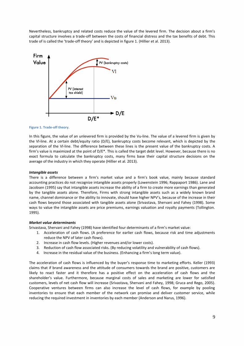
Nevertheless, bankruptcy and related costs reduce the value of the levered firm. The decision about a firm’s capital structure involves a trade-off between the costs of financial distress and the tax benefits of debt. This trade of is called the ‘trade-off theory’ and is depicted in figure 1. (Hillier et al. 2013).

Figure 1. Trade-off theory.

In this figure, the value of an unlevered firm is provided by the Vu-line. The value of a levered firm is given by the Vl-line. At a certain debt/equity ratio (D/E), bankruptcy costs become relevant, which is depicted by the separation of the Vl-line. The difference between these lines is the present value of the bankruptcy costs. A firm’s value is maximized at the point of D/E*. This is called the target debt level. However, because there is no exact formula to calculate the bankruptcy costs, many firms base their capital structure decisions on the average of the industry in which they operate (Hillier et al. 2013).

Intangible assets There is a difference between a firm’s market value and a firm’s book value, mainly because standard accounting practices do not recognize intangible assets properly (Lowenstein 1996; Rappaport 1986). Lane and Jacobsen (1995) say that intangible assets increase the ability of a firm to create more earnings than generated by the tangible assets alone. Therefore, Firms with strong intangible assets such as a widely known brand name, channel dominance or the ability to innovate, should have higher NPV’s, because of the increase in their cash flows beyond those associated with tangible assets alone (Srivastava, Shervani and Fahey (1998). Some ways to value the intangible assets are price premiums, earnings valuation and royalty payments (Tollington. 1995). Market value determinants Srivastava, Shervani and Fahey (1998) have identified four determinants of a firm’s market value:

1. Acceleration of cash flows. (A preference for earlier cash flows, because risk and time adjustments reduce the NPV of later cash flows).

2. Increase in cash flow levels. (Higher revenues and/or lower costs). 3. Reduction of cash flow associated risks. (By reducing volatility and vulnerability of cash flows). 4. Increase in the residual value of the business. (Enhancing a firm’s long term value).

The acceleration of cash flows is influenced by the buyer’s response time to marketing efforts. Keller (1993) claims that if brand awareness and the attitude of consumers towards the brand are positive, customers are likely to react faster and it therefore has a positive effect on the acceleration of cash flows and the shareholder’s value. Furthermore, because marginal costs of sales and marketing are lower for satisfied customers, levels of net cash flow will increase (Srivastava, Shervani and Fahey, 1998; Gruca and Rego, 2005). Cooperative ventures between firms can also increase the level of cash flows, for example by pooling inventories to ensure that each member of the network can promise and deliver customer service, while reducing the required investment in inventories by each member (Anderson and Narus, 1996).

10

Gruca and Rego (2005) have also found that risk associated with future cash flows is reduced when the firm has satisfied and loyal customers. The volatility of cash flows can be decreased when the relationship with customers and channel partners is positive. These relationships enable firms to coordinate their activities across the supply chain, which stabilized cash flows for all channel partners. Rappaport (1986) defines the residual value of the business as follows: ‘It reflects the expected value of the business beyond the planning horizon’. It is determined by the firm’s size, loyalty and quality of the customer base, which are all related to the satisfaction of this customer base (Srivastava, Shervani and Fahey, 1998), which will be discussed further in paragraph 2.2.3.

2.2.2 The media and investor sentiment Different researchers have tried to identify the effect of the media and investor sentiment on the stock market. Most theoretical models about investor sentiment and stock market pricing make two assumptions. First, they assume that there are two types of traders; noise traders and rational arbitrageurs. Second, they assume that both types of traders are risk averse (De Long et al., 1990). De Long et al. (1990) also claim that when noise traders experience a negative belief shock, they will sell the stocks to arbitrageurs, creating high volume trading. However, because these shocks are stationary, returns rebound the next period when there is a new belief shock. A conclusion they make is that ‘low sentiment will generate downward price pressure and unusually high or low values of sentiment will generate high volume’ (De Long et al., 1990). Tetlock (2007) found that high levels of media pessimism put downward pressure on market prices in the short run, followed by a reversion to original values. Furthermore, he claims that unusual high or low values of media pessimism forecast high trading volume. And lastly, he found that low market returns lead to a high level of pessimism in the media. Tetlock (2007) bases this on his analysis of the Wall Street Journal’s (WSJ) ‘abreast of the market’ column over a sixteen year period from 1984-1999. This column reviews the previous day’s movements on the stock market and tries to predict what will happen in the short term future. He chose the WSJ, because of three reasons. Firstly, the WSJ has over two million readers. Secondly, the WSJ has a strong reputation among investors. Thirdly, electronic texts of the columns are accessible over a long time horizon (Tetlock, 2007). Because all pessimistic news shocks only created a short-term price change, after which the prices returned to their original level, he concludes that the news articles did not provide new fundamentals that determine the value of the stocks. This means that the WSJ column only provides news that has already been implemented in the share price. One could also say that the market is therefore faster than the media. Even bolder is the conclusion of Cutler, Poterba and Summers (1989), who claim that important qualitative news stories do not even explain large market returns unaccompanied by quantitative macroeconomic events.

2.2.3 Customer satisfaction Firms who do well in the eyes of their customers, can be rewarded doubly; by more business from customers and more capital from investors as well (Mithas, S.; Fornell, C.; Forrest, V.M. & Krishnan, M.S., 2006). There is a significant relationship between customer satisfaction and market value of stock. Even so that the authors Mithas et al. (2006) claim that it is possible to beat the market consistently with consumer satisfaction based investment decisions. Fornell et al. (1996) say that firms with satisfied customers are rewarded by repeated business, greater market efficiency and lower price elasticity, which all lead to a growth in earnings and therefore a higher stock price. Heskett et al. (1997) go even further by claiming that customer satisfaction is positively associated with cost competitiveness, employee loyalty, profitable performance and long-term growth. The importance of growth has also been shown in the previous paragraph; to ensure continuity of a firm, managers must retain earnings to invest in growth opportunities (projects with positive NPV’s). Mithas et al. (2006) note that there is a possibility that news about increased customer satisfaction has a negative effect on the stock price, when the investors believe that the firm is giving away too much surplus to the buyers. Hereby, the investors think that the gap between the willingness to pay and the actual market price of a product might be too big, which leads to a lower than optimal income for the firm. Other situations where investors might react negatively to an increase in customer satisfaction is when the switching costs for the buyer are high, if there is a high degree of product differentiation or if there was some level of monopoly power (Mithas et al., 2006). Furthermore, there may be a reverse causality effect. This means that because dissatisfied customers are leaving the customer base and only the satisfied customers stay, the average level of satisfaction of the customer base increases, but a reduction in the amount of customers and sales occur also.

11

2.2.4 Macroeconomic factors Studies testing the relationship between, for example, oil prices and real stock returns suffer from two limitations. Firstly, many models assume that the oil price can be varied, while holding all other variables constant. This is not credible, because there is strong evidence that macroeconomic fluctuations have an influence in the price of oil as well as on the other variables (Kilian, 2007 & 2008). Secondly, the models assume that all shocks in oil prices are the same. However, some shocks are caused by macroeconomic factors and may influence the price of stocks directly themselves. Kilian & Park (2007) claim that in their study, they found that there are no simple and stable rules linking oil and stock prices; the relation depends on which shocks are driving the oil price. A change in macroeconomic variables can also affect many firms’ cash flows and can influence the used discount rates (Flannery and Protopapadakis, 2002). Several studies document that aggregate stock returns are negatively related to inflation and money growth (Bodie, 1976; Fama, 1981; Geske and Roll, 1983; Pearche and Roley, 1985). Chen, Roll and Ross (1986) have identified five potential macroeconomic factors that can influence equity returns: ‘the growth rate of industrial production’, ‘expected inflation’, ‘unexpected inflation’, ‘the default risk premium’ and a ‘term structure spread‘. Lamont (2000) concludes that especially portfolios that track the growth rates of industrial production, consumption and labor income provide abnormal positive returns. Also Cutler, Poterba and Summers (1989) confirm that growth in industrial production is positively correlated with stock returns. McQueen and Roley (1993) claim that changes in macroeconomic factors may have different effects, depending on the overall economic state. While an increase in employment might have a positive effect when the economy recovers from a recession, it might also have a negative effect when the economy is near its cyclical peak. Boyd, Jagannathan and Hu (2001) confirm that results might differ, depending on the economic state. They found that surprisingly high unemployment announcements raise stock prices during economic expansion, but lowers them during a contraction. The influence of macro-economic developments on a firm can be expressed as a firm’s beta regarding that specific macro-economic risk (Hillier et al. 2013). For example, when the share price of a firm is positively related to the risk of inflation, its inflation beta is positive and vice versa. If it’s uncorrelated with inflation, its inflation beta will be zero. Normally, when economists talk about a firm’s beta, they mean the standardized covariance of a stock’s return with the return on the market. The formula for calculating a firm’s beta is: beta i= Cov(Ri, Rm) / Var(Rm). Where the beta of share ‘i’ is the covariance of a share’s return ‘Ri’ with the return on the market ‘Rm’, divided by the market’s return variance (Hillier et al., 2013). When calculating a firm’s beta, it is important to use a sufficient amount of data, but ensure that all the data is actual, because macro-economic effects from the distant past may no longer represent current market conditions.

12

2.2.5 Commodities Since the beginning of the 1980’s, researchers started to investigate what they called the ‘commodity-stock market nexus’; the relation between these two markets. Khoury (1984) argues that unstable dividends, political risks, business risks and currency exchange risks disassociate the price of gold from the returns of the firm’s securities. Blose and Shieh (1995) have made a model that describes the influence of the gold price on the value of gold mining stocks. Their conclusion was that for companies whose primary business is gold mining, the elasticity of the stock and the gold price is greater than unity. However, there are also studies of the gold-stock market relationship that come up with different conclusions. Aggarwal and Soenen (1988) and Jaffe (1989) have found that the correlation between gold and the stock market is positive, but small. Tschoegl (1980), Carter et al. (1982), Larsen & McQueen (1995), Lawrence (2003) and McCown & Zimmerman (2006) even claim that gold is uncorrelated with the stock market. And then there is an author (Blose, 1996) who found that gold is negatively correlated with the stock market. Baur and Lucey (2010) have shown that gold serves as a good alternative for stocks in falling stock markets, as gold is uncorrelated with a portfolio of stocks in times of market stress. Considering crude oil price changes, the consensus of its precise effect on stock markets is not exactly clear neither. Kling (1985) finds that increases in the price of crude oil are associated with stock market declines. On the other hand, Chen et al. (1986) claim that changes in the oil price have no actual effect. Jones and Kaul (1996) found a negative, but stable, relation between changes in oil prices and aggregate stock returns, while Huang et al. (1996) did not find this negative relationship between stock returns and a change in the price of oil futures. As expected, a positive relation exists between the oil price changes and the oil and gas index or a combination of stocks of firms in the oil and gas industry (Sadorsky, 2001; Boyer and Filion, 2007). Miller and Ratti (2009) have analysed the long-term relation between the price of crude oil and international stock markets by using data from 1971-2008 and they found that there was an expected negative long-run relationship, which appears to have been disintegrated after 1999. They therefore suggest a change in the relationship between oil prices and stock prices since the turn of the century due to the presence of stock market or oil price bubbles. Algieri (2014) claims that the stock market has a magnified effect on commodity price returns. Creti et al. (2013) have investigated the correlation between 25 commodities and the S&P 500 index with data of the periods 2001-2011 and found that in many cases, the correlation has increased since 2007. They further claim that especially oil, coffee and cacao are characterized by a speculation phenomenon and while their correlations with the S&P 500 returns grow in times of increasing stock prices, they diminish in times of a bearish state of the market. Other researchers say that prior to the year 2000, agricultural commodity prices had little co-movements and correlations with financial prices (Gorton & Rouwenhorst, 2006). Buyukshain & Robe (2011, 2012) confirm that the level of commodity-equity linkages has fluctuated severely over the past two decades. They also claim that correlations between commodity futures and financial price returns have substantially increased since the last financial crisis and the demise of the Lehman Brothers in September 2008. Lehecka (2014) has found that since the start of the financialisation in agricultural commodity markets in 2004, food and financial markets exhibit greater co-movements and might even have integrated. The results are even stronger for the period since 2008.

13

3. Methodology This Chapter will describe the methodology used for the econometric analysis in this thesis. It will start with describing the procedure and will be followed up by a description of the data that has been used.

3.1 Model To test the relations between the commodity prices and stock prices, an ordinary least square regression (OLS) model will be estimated, whereby the firm’s stock is the dependent variable and the agricultural commodities, as well as the additional exogenous factors (crude oil prices, AEX and Debt-to-Equity ratios), are the independent variables. As showed in Table 1 on the next page, the different firms are expected to react to different commodities depending on their end products. To ensure that the models are compact and easy to interpret, only a selection of commodities is tested on their relation with the stock prices, based on the end products of the firm. This will be further elaborated in paragraph 3.2. To decide whether to run the OLS model with variables in first-difference or in levels, stationarity tests are performed on both dependent an independent variables. The test used was the Augmented-Dickey Fuller test (ADF). The intuition behind the ADF test is that if a series is stationary I(0), it has a tendency to return to a constant mean, which means that the level of the series is a good predictor of the next period’s change because of the presence of a unit root. However, if the series is integrated of an order greater than 0, shocks will occur with probabilities that do not depend on the current level of the series. After determining the stationarity of the variables, the appropriate lag order should be determined. It is expected that previous lags of the commodity prices can still affect current stock prices, due to the turnover period from buying raw materials to selling end products. To do this, the Akaike information criterion (AIC), Schwarz criterion (SC) and Hannan-Quinn criterion (HQ) have been calculated for a maximum of 11 lags (one year of price data). The results can be found in Table 2 in appendix B. Because the number of observations is quite large (+120), for all models except the ones of Nestlé and Unilever, the HQ is best used to identify the appropriate lag length (Venus & Liew, 2004). When the lag orders have been determined, the ordinary least squares (OLS) regression can be performed. The dependent variable and endogenous variables are put in the model, as well as the exogenous variables (AEX and D/E ratios). Eviews provides the coefficient estimates for all the variables and also shows the corresponding significance (probabilities). Furthermore, it provides the Durbin-Watson statistic (DW), which says something about the autocorrelations in the models. This statistic should be bigger than 2. If this is not the case, a further look is taken at the correlogram of the residuals and if necessary, autoregressive (AR) or moving averages (MA) terms are added to the model. Table 3 in appendix B provides suggestions of how to deal with different combinations of autocorrelations within a model. The elasticity’s of the different variables have been calculated as well, to see what the effect is of a 1% increase in commodity prices on the firm’s share price. The elasticity’s have been calculated by using the formula: Elasticity commodity ’x’ = Coefficient commodity ‘x’ * ( Average commodity ‘x’ price / Average share ’y’ price). The average price changes have been calculated by using the average function of Excel on the prices of the variables. The coefficients and elasticity’s will be discussed more extensively in Chapter 4. The financial statements of the firms have been used for explaining the results of the analysis, especially the firm’s risk management strategies regarding raw material price volatility. All firms have also been contacted by mail, to retrieve further information that could be useful for explaining the results. This information can all be found in appendix C.

14

3.2 Description of model variables Table 1 provides an overview with the different stocks and the specific agricultural commodities investigated. The explanation of why these combinations are made is provided below.

Table 1. Agricultural commodities expected to correlate with certain stocks

Dependent variables Independent variables

Nutreco Milk, Eggs, Maize, Sugar, Soybeans, Wheat Danone Milk, Eggs, Soybeans, Sugar Corbion Wheat, Oats, Barley, Rye, Sugar Bongrain Milk, Eggs, Soybeans, Sugar Unilever Milk, Eggs, Sugar Nestlé Milk, Eggs, Sugar, Soybeans, Wheat, Oats, Barley, Rye Bunge Wheat, Maize, Rice, Milk, Eggs, Sugar, Soybeans

Dependent variables: In this thesis, the stock prices of Nutreco, Danone, Corbion, Bongrain, Unilever, Nestlé and Bunge are the dependent variables. Nutreco’s mission is feeding the world’s growing population in a sustainable way. They process agricultural products, dairy products and marine products and should therefore react to price changes of the commodities milk, eggs, maize, sugar, soybeans and wheat. Danone is especially known for its dairy and nutrition products. Because of this, milk, sugar, egg and soybean price changes are expected to have a big impact on margin of Danone and the value of its shares. Corbion is a food processing group organized around 2 product groups. They are the number one provider worldwide for ingredients, semi-finished products, and finished products intended for bakeries, pastry chefs, and large distribution chains. The other product group consists of biochemical products, such as lactic acid and gluconic acid. Therefore, it can be expected that changes in cereal prices should have an effect on the firm’s stock price. Bongrain is the world's leading producer of cheese specialties. Net sales break down by family of products as follows: cheese products (59.8%), dairy products (39.9%), industrial dairy products (technical butters and specific dairy proteins for the food, dietetic, and health care industry, animal bottle feeding products) and dairy products for large-scale consumption (milk, modern butters, long-conservation creams, cheese desserts, etc.). The stock prices of Bongrain are expected to be related with the prices of milk, eggs, soybeans and sugar. Unilever has a couple of food and drink related products. Ben & Jerries ice cream and Becel spreads and cooking oil are examples of well-known brands and products. Therefore it can be expected that the firm’s stock prices are quite dependent on fluctuations in the prices of milk, eggs and sugar. Nestlé is committed to enhancing the quality of consumers’ lives through nutrition, health and wellness. They have a wide assortment of food related brands in the baby food, cereals, dairy, food, healthcare nutrition and pet care markets. They should therefore also be affected by changes in most of the commodity prices used in this thesis, namely milk, eggs, sugar, soybeans, wheat, oats, barley and rye. Bunge produces bottled oils, margarines, mayonnaises, flours and bakery products. They have a milling business where they create milled wheat, maize and rice products and the firm’s share prices should therefore also be related with the prices of these commodities. Furthermore, Bunge is a leading producer of sugar and ethanol in Brazil and a leading trader and merchandiser of sugar worldwide. In their current risk policy, they state that their business processes are therefore also dependent on sugar and soybean prices.

15

Additional exogenous variables Crude oil Because Kling (1985) finds that increases in the price of crude oil are associated with stock market declines and Jones and Kaul (1996) found a negative, but stable, relation between changes in oil prices and aggregate stock returns, the crude oil prices will also be used in all models, to see if anything can be said about the significance of oil price fluctuations on different shares. AEX As mentioned in Chapter 2, De Long et al. (1990) and Tetlock (2007)have tried to identify the effect of the media and investor sentiment on the stock market. A conclusion they make is that low sentiment will generate downward price pressure and unusually high or low values of sentiment will generate high volume. They also proof the market is faster in incorporating news shocks in the stock prices than the media. To take the macro-economic factors, such as inflation and news shocks into consideration, the AEX is used as an exogenous variable in the models.

Debt-to-equity ratios In Chapter 2, it has also been shown that the financial leverage of a firm has a direct influence on its market value and stock prices. Therefore, the D/E ratios have been implemented in the model as exogenous variables as well.

3.3 Data The commodities used in this thesis are agricultural commodities used by the food- and agribusiness. The monthly average European prices of the agricultural commodities and crude oil have been gathered for the period of 2000-2014 from the database of The World Databank and AGRIVIEW. All of these prices were found in euros, except the ones for sugar, which are manually converted form dollars to euros by using the monthly average exchanges rates for the period 2000-2014. Assuming that there were no arbitrage possibilities, these prices should reflect the true price the firms have had to pay during the periods. The daily closing prices for the stocks are gathered for the same period of 2000-2014, or a subset of this period for firms that where only listed on the stock market for a shorter period, from the Yahoo Finance database. From these prices, the monthly averages are taken, to make the prices comparable with the monthly averages of the commodity prices. All prices were found in euros, except the ones for Bunge, which were published in dollars. The monthly average exchange rates have been used to convert these prices into euros as well. The daily closing prices of the AEX have also been retrieved from the Yahoo finance website and of these prices, the monthly averages are taken as well. The yearly debt-to-equity (D/E) ratios have been retrieved or calculated from the firm’s financial statements from the years 2000-2014, which were published on the investor section on the webpages of the firms. The D/E ratios have been converted to monthly data by setting them fixed for each month in a certain year, since most of the financial statements were released only once a year. By performing an ADF test it has been found that, In this thesis, all variables, except milk, Corbion and eggs, are integrated of order 1, I(1), and therefore not stationary. Milk, Corbion and eggs have a unit root at a 5% significance level and are therefore integrated of order 0, I(0), and stationary. The statistics for the ADF tests can be found in appendix D. All variables in a model should be stationary and they can only be integrated with each other if they have the same order of integration. This means that for all the combination of commodities and firms in this thesis, the variables are not integrated. To achieve stationarity in the regression models, all variables have been first differenced.

16

4. Results This Chapter will describe the relations that have been found for all considered firms. Each firm will have its own paragraph. A table will be provided for each firm including the used variables, coefficients, probabilities, elasticity’s, DW statistic and the information criteria. These values have all been truncated at 4 decimals, to make the tables easier to read. The variables with a significant coefficient (probability <0.10) are marked by an ‘*’. From Table 2 in appendix B, it can be seen that in the models of Bunge, Corbion, Danone and Nutreco, Nestlé and Unilever, 0 lags should be included. For Bongrain, one lag will be included in the model. The information criteria provided in this Chapter can be used to compare the fit of the model with the fit of the models in Table 2 in appendix B. The models provided in this Chapter should have lower or equal values for the information criteria and therefore the best fit, compared with the different model options provided in Table 2. Some results will be coupled with information that could be found in the financial statements of the firms, regarding their procurement strategies. For readers interest, all received information about the firm’s procurement strategies can be found in appendix C.

4.1 Nutreco There are 0 lags added in Nutreco’s model and by looking at the Durbin Watson statistic (>2), it can be concluded that the model does not contain autocorrelation. Therefore, the model can be specified by the coefficients as presented in Table 4.1.

Table 4.1 Model Coefficients Nutreco

Variable Coefficient Prob. Elasticity

C 0.3833 0.0300*

D(CRUDEOIL) 0.0550 0.0353* 0.1795

D(MILK) -0.1702 0.1271 -0.3381

D(EGGS) 0.0028 0.8302 0.0193

D(SOYBEANS) -0.0048 0.4193 -0.0800

D(SUGAREURO) 12.7544 0.1194 0.3670

D(MAIZE) -0.0026 0.8411 -0.0268

D(WHEAT_PAN) 0.0109 0.3986 0.1113

D(AEX) 0.0102 0.0358* 0.2582

DENUTRECO -0.5006 0.1577

Akaike info criterion 3.2082

Schwarz criterion 3.3884

Hannan-Quinn criter. 3.2813

Durbin-Watson stat 2.1091

Table 4.1 gives the coefficients of all one period lagged differences of the independent variables and provides information whether their impact on the change in Nutreco’s share prices is significant or not. The coefficients that are significant at the critical 5% level (prob. <0.05) are the ones of Crude oil and the AEX. This means that when the price of crude oil increases with €1, the share price of Nutreco increases with €0.055. This effect is quite unexpected, since Nutreco’s business processes are initially not related with the prices of oil. Another interesting fact is that in 2015, Nutreco has been bought by SHV, a Dutch investment company that owns assets in oil exploration and transport as well. Because the data used in this regression is from before this acquisition, the business of Nutreco was not yet integrated with the business of SHV, so there should be another factor that links Nutreco with the crude oil prices.

17

Skretting is a Nutreco owned company that provides nutritional solutions for the aquaculture industry. It has published a press release in 2008 in which they say the following: ‘More fishmeal is being bought again, for example by the Chinese pig producers, and fish oil prices are being buffeted by the effects of biofuel production and crude oil prices together with an increasing demand for omega-3 supplements and capsules’ (Skretting, 2008). Because Skretting is a company owned by Nutreco, the linkage between the fish oil market and the crude oil market might turn out to be a significant factor to influence the share price of Nutreco. The elasticity of crude oil is 0.1795, implying a 0.1795% increase in Nutreco’s share price as a result of a 1% increase in crude oil prices. The model also implies that when the AEX index increases with 1 point, Nutreco’s share price increases with €0.0102. The elasticity of the AEX is 0.2582, which implies that when the AEX increases with 1%, the share price of Nutreco increases with 0.2582%. This means that Nutreco has a positive beta regarding the AEX and tends to profit from a positive economic climate. The financial statements of Nutreco provide the information that Nutreco has contracts with their suppliers and customers, which allow the firm to transmit raw material price changes to the selling price of their products. If they are successful in maintaining their margin more or less constant, then it can also be explained why most of the price changes of the raw materials do not significantly affect Nutreco’s share price.

4.2 Bongrain There is 1 lag of each variable incorporated in the model, as was suggested by the information criteria. By looking at the Durbin Watson statistic (>2), it can be concluded that the model does not contain autocorrelation. The model coefficients are provided in Table 4.2. Table 4.2 Model Coefficients Bongrain


C 0.2355 0.7281

D(CRUDEOIL) -0.0060 0.9318 -0.0075

D(EGGS) -0.0008 0.9834 -0.0020

D(MILK) -0.5532 0.1622 -0.4161

D(SOYBEANS) -0.0004 0.9770 -0.0027

D(SUGAREURO) 5.1564 0.8089 0.0562

D(AEX) 0.0295 0.0207* 0.2826

D(BONGRAIN(-1)) -0.2447 0.0012* -0.2447

D(CRUDEOIL(-1)) -0.1131 0.1113 -0.1399

D(EGGS(-1)) -0.0809 0.0257* -0.2110

D(MILK(-1)) 0.2822 0.5091 0.2122

D(SOYBEANS(-1)) 0.0089 0.5431 0.0559

D(SUGAREURO(-1)) -5.3233 0.8077 -0.0580

D(AEX(-1)) 0.0462 0.0004* 0.4422

DEBONGRAIN 0.3392 0.8063





18

From this table it can be concluded that the variables D(AEX), D(Bongrain(-1)), D(Eggs(-1)) and d(AEX(-1)) have a significant effect on the difference in Bongrain’s share price (Prob. <0.05). This means that the current difference in the AEX and the difference of one lag ago can partly explain the current price change in Bongrain’s share prices. This also counts for the price difference in Bongrain’s share price of one lag ago and the change in egg prices one lag ago. The coefficient for the current change in the AEX, implies that Bongrain’s share price will increase with €0.0295 when the AEX index increases with 1 point. This shows that the beta of Bongrain regarding the AEX is positive and that Bongrain tends to thrive in a positive economic climate. This is confirmed by the coefficient of the one lagged difference in the AEX index (0.0462). The elasticity’s of the current AEX difference and the AEX difference of one lag ago are in line with the coefficients. Both elasticity’s imply a positive relation between the AEX and Bongrain. A 1% increase in the AEX of one lag ago, results in a 0.4422% increase in Bongrain’s share price and a 1% increase in the current AEX, results in an increase of 0.2826% in Bongrain’s share price. The coefficient for the one lagged difference in Bongrain’s share prices, show that when there has been an increase in the share price of €1, the share shows a little correction of -€0,2447 a month later. This is in line with the theory that share prices tend to correct after a price shock has occurred (De Long et al., 1990). The one lagged price difference of eggs also has a significant coefficient. This implies that when the egg prices increased with €1,- one month ago, the current share price of Bongrain decreases with €0.0809. It very likely that Bongrain uses eggs as input for their food products and that an increase in these prices will result in a lower margin for Bongrain. Therefore it is also likely that the share price decreases a little. The elasticity for the one lagged price difference in eggs is -0.2110. This implies that when the egg prices increased one month ago with 1%, the current share price of Bongrain decreases with 0.211%. This is in line with the coefficient found for this variable. It was also expected that Bongrain’s shares would react strongly to milk prices, since this is the main raw material used to produce cheese products. The coefficient for this variable is however insignificant. The current milk price difference has a probability of 0.16, which is outside the 10% limit. The reason that this variable is insignificant, could be because of Bongrain’s successful hedging strategies. In a correspondence by email with one of the managers of Bongrain, he said that: ‘Regarding milk, our policy is to develop specialties products and/or value added industrial products which are less impacted by the commodity prices.’ Furthermore, there was a milk quota in the EU during the researched period, with as goal to limit the volatility in milk prices. Therefore, almost no volatility in milk prices could be observed, while the share price of Bongrain had the ability to be more volatile.

19

4.3 Bunge The information criteria suggested to add 0 lags in Bunge’s model. However, this resulted in a model with a Durbin Watson statistic <2, so it can be concluded that there is some form of autocorrelation in the model. Therefore a further check is performed by looking at the correlogram of Bunge’s residuals which can be found in appendix B. The correlogram shows one or more spikes and therefore a moving average model is indicated. The partial autocorrelations are difficult to interpret. However, the highest DW statistic is found by including a MA(1) and MA(3) term in the model. This results in the new coefficients found in Table 4.3 below. The Durbin Watson statistic is now bigger than 2, which means that the autocorrelation is taken out of the model.

Table 4.3 Model Coefficients Bunge (corrected for autocorrelation)


C 0.0102 0.9794

D(CRUDEOIL) 0.0891 0.0949* 0.1118

D(WHEAT_PAN) 0.0050 0.8728 0.0198

D(MAIZE) 0.0231 0.4717 0.0905

D(RICE) 0.0097 0.2437 0.0706

D(EGGS) 0.0171 0.4958 0.0451

D(MILK) 0.2068 0.4399 0.1578

D(SOYBEANS) 0.0135 0.2973 0.0856

D(SUGAREURO) 51.3853 0.0055* 0.5681

D(AEX) 0.0717 0.0000* 0.6965

DEBUNGE 0.7415 0.2557

MA(1) 0.3806 0.0000*

MA(3) -0.3781 0.0000*





The coefficients show that the current price change of sugar is highly significant (Prob. <0.01) with a value of 51.3853. This would suggest that when the sugar price increases with 1 eurocent per kg, the share price of Bunge would increase with 51.3853 eurocents. Reason for this positive relationship is that Bunge is a leading producer and merchandiser of sugar worldwide. When sugar becomes more valuable, this means that one of Bunge’s products becomes more valuable. The elasticity backs up this positive relation with a value of 0.5681. This means that when the sugar price increases with 1%, the share price of Bunge increases with 0.5681%. The moving averages of one and three months are also highly significant. It seems that their effects cancel out, because the coefficients values are almost equal and the one for a moving average of three months has a negative impact while the moving average of one month has a positive impact. This might be explained by the time it takes for Bunge to transmit changes in raw materials to their selling prices. The change in the AEX is also highly significant and provides a coefficient of 0.0717. This means that when the AEX increases with 1 point, the share price of Bunge increases with €0.0717. The elasticity of the AEX is 0.6965, which would suggest that when the AEX increases with 1%, Bunge’s share price would increase with 0.6965%.

20

Crude oil price differences are significant on a 10% level, with a p-value of 0.0949. The coefficient is 0.0891, which implies an increase in Bunge’s share price of €0.0891 when the crude oil price rises with €1. The elasticity of crude oil is 0.1118, which implies a 0.1118% increase in Bunge’s share price, when the crude oil price rises with 1%. The reason why an increase in oil prices also results in an increase in Bunge’s share price is because Bunge is a leading producer of ethanol, a substitute for oil. So when oil becomes more expensive, substitutes such as ethanol become more interesting/valuable for buyers. In Bunge’s risk management policy, they mention soybeans, wheat, corn and sugar as their main raw material purchases. It is therefore remarkable that only sugar has a significant impact. In the risk policy it is also stated that the firm enters into various derivative contracts to limit the risk of exposure to adverse price movements in the commodities they use for their operations. The results of the regression performed in this thesis show that Bunge is very successful in minimizing their exposure to risk of price volatility in agricultural products..

4.4 Corbion There are 0 lags added in Corbion’s model and by looking at the Durbin Watson statistic (>2) it can be concluded that there is no autocorrelation in the model. The coefficients can therefore be specified as in Table 4.4. Table 4.4 Model Coefficients Corbion


C -0.1381 0.5007

D(CRUDEOIL) 0.0500 0.1053 0.1554

D(WHEAT_PAN) 0.0159 0.5379 0.1552

D(OATS) 0.0023 0.8948 0.0178

D(BARLEY_BRAS) -0.0222 0.2918 -0.2230

D(RYE_PAN) 0.0053 0.7646 0.0446

D(SUGAREURO) 4.9775 0.6152 0.1364

DECORBION 0.1912 0.4318

D(AEX) 0.0148 0.0173* 0.3565





The conclusion can be drawn that only the AEX explains Corbion’s share price significantly (P value <0.05). The coefficient of the first difference in the AEX index is 0.0148. Which implies a very small, positive beta. The elasticity regarding the AEX is 0.3565, which implies that when the AEX index increases with 1%, the share price of Corbion increases with 0.3565%. Unfortunately, as a reaction to the inquiry by mail to Corbion for an elaboration on their raw material purchasing policy they responded that they could not disclose this information due to the sensitivity of that information.

21

4.5 Danone There are 0 lags added in Danone’s model and by looking at the Durbin Watson statistic (>2) it can be concluded that there is no autocorrelation in the model. Therefore the coefficients provided in 4.5 are valid. Table 4.5 Model Coefficients Danone


C 0.5667 0.1387

D(CRUDEOIL) 0.0187 0.6561 0.0287

D(MILK) -0.0723 0.6819 -0.0673

D(EGGS) 0.0125 0.5553 0.0404

D(SOYBEANS) -0.0141 0.1093 -0.1092

D(SUGAREURO) 8.5563 0.5196 0.1153

D(AEX) 0.0232 0.0033* 0.2747

DEDANONE -0.4840 0.3779





From Table 4.5, It can be concluded that none of the commodity price changes can explain Danone’s share price significantly. Only the change in the market (AEX) is highly significant (p-value <0.01). The coefficient regarding the AEX is 0.0232, which implies that when the AEX index increases with 1 point, the share price of Danone increases with €0.0232. Therefore, it can be said that Danone also thrives better in a positive economic climate. The elasticity for the AEX is 0.2747, which means that when the AEX index increases with 1%, the share price of Danone increases slightly with 0.2747%. This is in line with the coefficient found for this variable. Since Danone is well known for its dairy products, it is remarkable that the share price are not significantly affected by milk price changes. A reason for this could be their successful risk management strategy regarding the purchase of raw products. In the firm’s risk management policy, they name milk as their leading raw material purchased by the Danone group. The firm’s operating subsidiaries generally enter into supply agreements with local producers and cooperatives. The price is set locally in periodical contracts that vary in length depending on the country. Furthermore, there was a milk quota in the EU during the researched period, with as goal to limit the volatility in milk prices. Therefore, only a little volatility in milk prices could be observed, while the share price of Danone had the ability to be more volatile.

4.6 Nestlé As suggested by the information criteria, there are 0 lags added in Nestlé’s model. However, this results in a model with a Durbin Watson statistic <2. Therefore, it can be concluded that there is autocorrelation in the model. A further check is performed by looking at the correlogram of Nestlé’s residuals, which can be found in appendix B. The correlogram does not clearly show any pattern of residuals significantly bigger than 0, although it seems that lag 11 crosses the significance limit. Therefore an AR(11) term is included in the model. This still results in a DW statistic below 2. The new correlogram now implies a moving average, that decays to 0 after the fourth lag. Therefore an MA(4) term is also included in the model. This results in the coefficients estimations reported in Table 4.6. The DW statistic is now bigger than 2, so it can be concluded that the model does no longer contain any autocorrelations.

22

Figure 4.6 Model Coefficients Nestlé (corrected for autocorrelation)


C 1.3763 0.0001* D(CRUDEOIL) -0.0744 0.0929* -0.1013

D(EGGS) 0.0419 0.0018* 0.1204

D(MILK) -0.5804 0.0030* -0.4808

D(SUGAREURO) 1.8040 0.8603 0.0217

D(SOYBEANS) 0.0143 0.0403* 0.0989

D(WHEAT_PAN) 0.0115 0.6687 0.0491

D(OATS) -0.0154 0.3080 -0.0523

D(BARLEY_BRAS) 0.0385 0.0739* 0.1690

D(RYE_PAN) -0.0425 0.0393* -0.1572

D(AEX) 0.0266 0.0070* 0.2803

DENESTLE -3.5991 0.0071* AR(11) -0.5957 0.0000* MA(4) -0.9059 0.0000*





The coefficients that are significant are the price change of crude oil (on a 10% basis), the price change of soybeans, barley and rye (on a 5% basis) and the price change in eggs, milk, the AEX, the D/E ratio and the AR and MA terms (on a 1% basis). The coefficient for crude oil (-0.0744) implies that when the crude oil price increases with €1, the share price of Nestlé decreases with €0.0744. This negative relationship might be explained by the fact that plastic is Nestlé’s primary packaging material and it is made from a by-product of crude oil. Therefore, when crude oil becomes more expensive, the packaging material for Nestlé will also become more expensive. This negative relation is in line with the elasticity for crude oil (-0.1013). It implies that when crude oil prices rice with 1%, the share price of Nestlé decreases with 0.1013%. For eggs, the coefficient is 0.0419. This means that when the prices of eggs increase with €1, the share price of Nestlé will increase with €0.0419. The elasticity of 0.1204 also shows that there is a positive relation between the prices of eggs and the share price of Nestlé. It implies that when egg prices rise with 1%, the share price of Nestlé increases with 0.1204%. This might be explained by the fact that Nestlé produces a lot of nutrition products. One of the nutrition basics is proteins, which can be retrieved from eggs. If eggs become more valuable, the proteins also become more expensive. The coefficient and elasticity show that Nestlé is quite successful in benefiting from these price changes. For soybeans, the model provides a positive coefficient of 0.0143, which implies that when soybean prices increase with €1, Nestlé’s share price will increase slightly with €0.0143 and it has a positive elasticity of 0.0989 as well. The same reasoning for this positive relation could be applied here, since soybeans are a good provider of other nutrition basics such as calcium, magnesium and iron. The coefficient for barley is also positive (0.0385), meaning that a €1 increase in barley prices will trigger an increase of €0.0385 in the share price of Nestlé. The elasticity is 0.1690. According to the website of Nestlé, barley is a good provider of soluble fibres. The positive relation between barley and Nestlé’s share price could therefore also be explained by the same reasons that apply to eggs and soybeans.

23

The coefficient for milk implies that a €1 increase in the prices of milk will result in a decrease of €0.5804 in the share price of Nestlé. The elasticity implies that a 1% increase in milk prices results in an 0.4808% decrease in Nestlé’s share price. The reason for this negative relationship could be the usage of milk as a raw material for the dairy products that Nestlé produces. It is however remarkable that, even though the milk quota was also active in the EU during the researched period of Nestlé, it still has a significant relation with the milk price. This is in contrast with the results for Bongrain and Danone, who also use milk as raw material. For a €1 increase in rye prices, the effect will be a decrease of €0.0425 in Nestlé’s share price and for a 1% increase in rye prices, Nestlé’s share price will decrease with 0.1572%. This negative relation might be explained by the usage of rye in Nestlé’s cereal products. The coefficient for the AEX is 0.0266. This means that when the AEX increases with 1 point, the share price of Nestlé will increase with €0.0266. The elasticity of the AEX, which is 0.2803, implies that when the AEX increases with 1%, the share price of Nestle increases with 0.2803%. For the D/E ratio, the coefficient is -3.599. This implies that when the D/E ratio increases with 1 (the debt increases or the equity decreases), the share price of Nestlé will decrease with €3.599. As described in Chapter 2 of this thesis, this means that taking on extra debt results in a higher risk of financial distress for Nestlé than it gains in tax benefits. Only little information could be found on the procurement strategies of Nestlé. The firm states that they have over 600.000 small scale suppliers whit whom they hold close contact. Furthermore, the firm enters into future contracts as well, but this information is not disclosed publicly.

4.7 Unilever There are 0 lags added in Unilever’s model, but this results in a model with Durbin Watson statistic <2. Therefore, it can be concluded that there is autocorrelation in this model. A further check is performed by looking at the correlogram of Unilever’s residuals, which can be found in appendix B. The correlogram shows one or more spikes and therefore a moving average model is indicated. The partial autocorrelations show that the order at which the plot becomes 0 is after the third one. Therefore a MA(3) term is included in the model. This results in new coefficients, but the DW is still lower than 2. The new correlogram shows that the residuals of lag 1 and 5 are just outside of the 0 range and therefore an AR(1) and AR(5) term are also included in the model. This results in the coefficients found in Table 4.7.

Table 4.7 Model Coefficients Unilever


C 0.4868 0.0686*

D(CRUDEOIL) 0.0403 0.0188* 0.1024

D(MILK) -0.1676 0.0349* -0.2592

D(EGGS) 0.0026 0.7346 0.0138

D(SUGAREURO) -2.1144 0.6779 -0.0474

D(AEX) 0.0220 0.0000* 0.4343

DEUNILEVER -0.5282 0.2417

AR(1) 0.3300 0.0015*

AR(5) -0.2758 0.0077*

MA(3) -0.4674 0.0000*





24

The coefficients as represented in Table 4.7.3, show that the current price changes in crude oil, milk and AEX are all significant with p-values <5. This means that when the milk price increases with €1, the share price of Unilever will decrease with €0.1676. This is expected, because Unilever probably uses milk as a raw product in their business processes. So when the price of this raw product increases, it will lower their margin and therefore also the value of the shares. This is backed up by the elasticity of -0.2592, which implies that when milk becomes 1% more expensive, the share price of Unilever drops with 0.2592%. The significant relation with volatility in milk prices is remarkable, since there was a milk quota during the researched period, aiming to limit volatility in milk prices. When the price of crude oil increases with €1, the share price of Unilever will increase with €0.0403. This is unexpected, since Unilever would likely only use crude oil for transportation purposes and the by-product of crude oil for their plastic packaging material. Therefore one would expect that when the crude oil price increases, these costs of Unilever would also increase. This should result in a lower margin and therefore also a lower share price. The elasticity backs up the positive relation between crude oil and Unilever, providing that a 1% increase in crude oil prices results in a 0.1024% increase in Unilever’s share price. Information provided by Unilever was not sufficient enough to further explain this positive relationship. The Table also shows that the coefficient of Unilever towards the AEX is 0.0220. Which means that Unilever shares will increase with €0.0220, when the AEX increases with 1 point. This in agreement with the elasticity for the AEX, which is 0.4343. This implies that when the AEX increases with 1%, the share price of Unilever will decrease with 0.4343%.

25

5. Discussion The results of this study show limited relationships between agricultural commodity prices and stock prices. Other researchers say that prior to the year 2000, agricultural commodity prices had little co-movements and correlations with financial prices (Gorton & Rouwenhorst, 2006). This thesis used data from 2000 and onwards and it seems that there still are little co-movements and correlations with share prices, provided that the firms use hedging strategies to provide them with time to transmit price fluctuations of raw material to their selling prices. Lehecka (2014) has found that since the start of the financialisation in agricultural commodity markets in 2004, food and financial markets exhibit greater co-movements and might even have integrated. The results are even stronger for the period since 2008. It is interesting to note that for Nestlé, the firm with the most significant relations with the commodities, the data used in this thesis is from 2008 and onwards. Although only one case is too little to make definite statements about this hypothesis, it could be an interesting fact for other researchers to only look into price relations from the period 2008 and onwards and see if this hypothesis can be further proven. Similar to the results of this thesis, the literature does not provide any consensus on the relation between crude oil prices and stock markets neither. As described in Chapter 2.2.5, Kling (1985) finds that increases in the price of crude oil are associated with stock market declines, while Chen et al. (1986) claim that changes in the oil price have no actual effect. Miller and Ratti (2009) have analysed the long-term relation between the price of crude oil and international stock markets by using data from 1971-2008 and they found that there was an expected negative long-run relationship, which appears to have been disintegrated after 1999. They therefore suggest a change in the relationship between oil prices and stock prices since the turn of the century due to the presence of stock market or oil price bubbles. Since the data used for this thesis is from 2000 and onwards, it could be used by other researchers as a beginning for the follow up research of Miller and Ratti. There are a few limitations in this thesis. One of which is the usage of monthly averages instead of daily closing prices of the variables. The reason why monthly averages have been used is that this data was already available for the commodities. This meant that only the stock price data had to be collected, which is widely accessible online. Because of the usage of monthly averages, short term day to day fluctuations could not be observed. It is expected though that firms and speculators do react instantly when a shock occurs, so using daily price data could result in more observable volatility and significant relations than using monthly averages. This introduces the second limitation of this thesis; only few significant relations have been found. In the empirical framework, some factors that influence share prices have been provided. The market factors, implemented in the model with the AEX variable, are indeed significant for all firms. The D/E ratios are however only significant for Nestlé. Reason for this can be explained by the fact that the ratios were only available on a yearly basis, while the model assumes monthly periods. By setting the ratios fixed for each month, only changing them during the first month of the next year, very little volatility could be observed. If other researchers wish to take a closer look at the relation between a firm’s D/E ratio and the share prices, it would be suggested to take the yearly average stock prices and ratios of the firms for a longer period and regress the model with these yearly averaged prices to check the relation between these variables for each specific firm. Another option for follow up research is to look at the interrelations of the independent variables as well. It is expected that the agricultural commodities have relations with each other. For example, sugar and corn can both be used to produce ethanol and are therefore substitutes of each other. Which would also imply that the prices of these commodities react to one another. The data of this thesis could be used to estimate different vector-autoregressive (VAR) models and a further analysis on those coefficients could be performed.

26

6. Conclusion The objective of this thesis was to gain more knowledge about the relation between volatility in agricultural commodity prices and volatility in food corporations’ stock prices. It was expected that the commodity prices would influence the margins and cash flows of firms in the food- and agribusiness and thereby affect the share prices of those firms as well. This hypothesis was however not strongly supported by the performed analysis. As an answer to the first research question, ‘what factors determine a corporation’s share price in theory?’, the performed literature study provided multiple influential factors. First of all, share prices are determined by dividing the expected future dividends by the discount rate; P0=∑Divt/(1+Rt)

t. Other factors that can influence

the market value of shares are: the financial structure of the firm, the media, investor sentiment, customer satisfaction, macro-economic factors and commodity prices. During the process of answering the second research question, ‘what is the correlation between stock prices and commodity prices?’, the econometric analyses did only show a poor correlation or no correlation at all between the stocks and commodities. For example, Nutreco is a firm that processes agricultural and dairy products. It was therefore expected that they are quite dependent on the price fluctuations of milk and cereals. The data suggested however that only the price fluctuations of crude oil did significantly explain changes in the share price of Nutreco. Another example is Danone. Danone is very well known for its dairy and nutrition products and therefore expected to be related with milk and sugar prices. The data found in this thesis does however provide no significant relations between the commodity prices and the share price of Danone. This applies to Corbion as well. The insignificance of most of the commodities in regard to most of the firms can partly be explained by the successful hedging strategies of those firms. Although most of the firms are not very explicit about their hedging strategies, some information was retrieved from their financial statements. Nutreco has, for example, raw material contract positions, which are based on its business models. Furthermore, they transmit most of the raw material prices to the selling prices directly. This ensures them that their margins stay more or less constant. Danone states in its financial statements that milk is their main raw material need, as was expected on beforehand as well. They enter into supply agreements with local producers and cooperatives and set the price over contractual periods that differ per country. For its other raw material need, such as sugar, they secure price-setting with suppliers or hedge by using derivative markets. The results of this thesis could be used as a stepping stone to take a closer look at the effect of price risk management strategies on the share prices of stock listed food companies. A firm that does have strong relations with the commodity prices is Nestlé. This firm is one of the biggest firms in the food industry with products for the baby food, cereals, dairy, food, healthcare, nutrition and pet care markets. Therefore, it was also expected that Nestlé would strongly depend on most of the commodity prices used in this thesis. In the case for Nestlé, the data does really support this hypothesis. It provided significant values for changes in soybeans, barley, rye, eggs and milk prices. However, the model suggested positive relations for eggs, soybeans and barley, while it suggested negative relations for crude oil, milk and rye. It is interesting though that for the firm that proved to be most dependent on commodity price volatility (Nestlé), also very little information regarding their risk management policy could be found. Information that the firm provides is that they purchase their main raw materials directly from over 600.000 small-scale suppliers. It can be expected that Nestlé has quite some bargaining power over these small suppliers, but it seems that the hedging effectiveness of this strategy is not very solid. Regarding the significance of crude oil on the share prices, its effect is still not exactly clear. The data suggests a positive relation with Nutreco’s, Unilever’s and Bunge’s share prices, while a negative relation with Nestlé’s share price. Furthermore the prices of crude oil seem uncorrelated with the share prices of Danone, Corbion and Bongrain.

27

References Aggarwal, R. & Soenen, L.A. (1988). The Nature and Efficiency of the Gold Market. J. Portfoilio Manag. 14, 217-

229. Algieri, B. (2014). The Influence of Biofuels, Economic and Financial Factors on Daily Returns of Commodity

Futures Prices. Energy Policy 69, pp. 227–247 Altman, E.I. (1984). A Further Empirical Investigation of the Bankruptcy Cost Question. Journal of Finance 39,

1067-1089. Anderson, James C. & Narus, J.A. (1996). Rethinking Distribution: Adaptive Channels. Harvard Business Review

74, 112-22. Antweiler; Werner, & Frank. (2004). Is All That Talk Just Noise? The Information Content of Internet Stock

Message Boards. Journal of Finance 59, 1259–1293. Bardaji, M., Garrido, A., Iglesias, E., Blanco, M. & Bielza, M. (2011). What Market Measures in the Future CAP

After 2013? Barker, R.; Clubb, C.; Hendry, J.; Imam, S.; Roberts, J. & Sanderson, P. (2008). The Use of Valuation Models by

UK Investment Analysts. European Accounting Review 17, 503-535. Baur, D.G. & Lucy, B.M. (2010). Is Gold a Hedge or a Safe Haven? An Analysis of Stocks, Bonds and Gold.

Financial Review 45, 217-229. Blose, L.E. (1996). Gold Price Risk and the Returns on Gold Mutual Funds. J. Econ. Bus. 48, 499-513. Blose, L.E. & Shie, J.C.P. (1995). The Impact of Gold Price on the Value of Gold Mining Stock. Rev. Financ.

Econom. 4, 125-139. Bodie, Z. (1976). Common Stocks as a Hedge Against Inflation.Journal of finance 3, 359-470. Boyd, J.H.; Jagannathan, R. & Hu, J. (2001). The Stock Market’s Reaction to Unemployment News: Why Bad

News is Usually Good for Stocks. Working Paper 8092, NBER. Boyer, M.M. & Fillion, D. (2007). Common and Fundamental Factors in Stock Returns of Canadian oil and Gas

Companies. Energy Econ. 29, 428-453. Buyuksahin, B. & Robe, M.A. (2011). Does ‘Paper-Oil’ Matter? Energy Markets’ Financialization and Equity-

Commodity Co-movements. Working Paper. Buyuksahin, B. & Robe, M.A. (2012). Speculators, Commodities and Cross-Market Linkages. Working Paper. Carter, K.J., Affleck-Graves, J.F. & Money, A.H. (1982). Are Gold Shares Better Than Gold for Diversification?. J.

Portfolio Manag. 9, 52-55. Chen, N.F.; Roll, R. & Ross, S. (1986). Economic Forces and the Stock Market. Journal of business 59, 383-403. Creti, A., Joets, M. & Mignon, V. (2013). On the Links Between Stock and Commodity Markets’ Volatility. BIS Q.

Rev, 53-67. Cutler, D.M.; Poterba, J.M. & Summers, L.H. (1989). What Moves Stock Prices? Journal of Portfolio

Management 15, 4–12. De Long, J.; Bradford, S.; Summers, L.H. & Waldmann, R.J. (1990). Noise Trader Risk in Financial Markets.

Journal of Political Economy 98, 703–738. Fama, E. (1982). Stock Returns, Real Activity, Inflation, and Money. American Economic Review 71, 545-565. Ferris, K. & Petitt, B. (2013). Valuation for Mergers and Acquisitions: An Overview. Financial Times Press. Flannery, M.J. & Protopapadakis, A.A. (2002). Macroeconomic Factors Do Influence Aggregate Stock Returns. Fornell, C.; Johnson, M.D.; Anderson, E.W.; Cha, J. & Bryant, B.E. (1996). The American Customer Satisfaction

Index: Nature, Purpose, and Findings. Journal of Marketing, 60 (October), 7-18. Geske, R. & Roll, R. (1983). The Fiscal and Monetary Linkage Between Stock Returns and Inflation. Journal of

finance 38, 1-34. Gruca, T. & Rego, L. (2005). Customer Satisfaction, Cash Flow, and Shareholder Value. Journal of Marketing, 69

(July), 115-30. Gorton, G.B. & Rouwenhorst, K.G. (2006). Facts and Fantasies About Commodity Futures. Financial Analysis

Journal 62, 47-68. Hamilton, J. (2009). Causes and Consequences of the Oil Shock of 2007-2008. Working Paper, UC San Diego. Heskett, J.L.; Sasser, W.E. & Schlesinger, L.A. (1997). The Service Profit Chain: How Leading Companies Link

Profit and Growth to Loyalty, Satisfaction and Value. New York: The Free Press. Hillier, D.; Ross, S.; Westerfield, R; Jaffe, J. & Jordan, B. (2013). Corporate Finance. 2nd European Edition. Huang, R., Masulis, R., & Stoll, H. (1996). Energy Stocks as Investments for Institutional Portfolios. Financial

Analysis Journal 45, 53-59. Jones, C. & Kaul, G. (1996). Oil and the Stock Markets. J. Finance 51, 463-491. Keller, K.L. (1993). Conceptualizing, Measuring, and Man- aging Customer-Based Brand Equity. Journal of

Marketing, 57 (January), 1-22. Khoury, S.J. (1984). Speculative Markets. MarcMillan, New-York.

28

Kilian, L. (2007). Not All Oil Price Shocks Are Alike: Disentangling Demand and Supply Shocks in the Crude Oil Market. University of Michigan. Available at: http://www-personal.umich.edu/~lkilian/paperlinks.html

Kilian, L. (2008). Exogenous Oil Supply Shocks: How Big Are They and How Much Do They Matter for the US Economy? Review of Economics and Statistics

Kilian, L. & Park, C. (2007). The Impact of Oil Price Shocks on the U.S. Stock Market. University of Michigan. Kilian, L. (2009). Not All Oil Price Shocks Are Alike: Disentangling Demand and Supply Shocks in the Crude Oil

Market. American Economic Review 99, 1053-69. Kling, J.L. (1985). Oil Price Shocks and Stock-Market Behavior. J. Portfolio Manag. 12, 34-39. Krugman, P. (2008). Fuels on the hill. The New York Times 27. Lamont, O. (2000). Economic Tracking Portfolios. Journal of Econometrics 105, 161-184. Lane, V. & Jacobsen, R. (1995). Stock Market Reactions to Brand Extension Announcements: The Effects of

Brand Attitude and Familiarity. Journal of Marketing 59, 63-77. Larsen, A.B. & McQueen, G.R. (1995). REITs, Real Estate, and Inflation Lessons From the Gold Market. J. Real

Estate Finance Econ. 10, 285-297. Lawrence, C. (2003). Why is Gold different From Other Assets? An Empirical Investigation. London, UK: World

Gold Council. Lehecka, G.V. (2014). Have Food and Financial Markets Integrated? Vienna: University of Natural Resources

and Life Sciences. Lombardi, M. & Van Robays, I. (2011). Do Financial Investors Destabilize the Oil Price? European Central Bank

Working Paper 1346. Lowenstein, R.F. (1996). The 'Q': ‘When Is a Burger Not a Burger'? The Wall Street Journal. McCown, J.R. & Zimmerman, J.R. (2006). Is Gold a Zero-Beta Asset? Analysis of the Investment Potential of

Precious Metals. Social Science Research Network Working Paper, 920396. McQueen, G. & Roley, V. (1993). Stock Prices, News, and Business Conditions. Review of financial studies 6, 683-

707. Miller, J.I. & Ratti, R.A. (2009). Crude Oil and Stock Markets: Stability, Instability and Bubbles. Energy Econ. 31,

559-568. Mithas, S.; Fornell, C.; Forrest, V.M. & Krishnan, M.S. (2006). Customer Satisfaction and Stock Prices: High

Returns, Low Risk. Journal of Marketing Vol 70. pp 3-14. Modigliani, F. & Miller, M.H. (1958). The Cost of Capital, Corporation Finance and the Theory of Investment. The

American Economic Review 48, 261-297. NIST/SEMATECH (2003). e-Handbook of Statistical Methods. Used on 17-03-2015, from:

http://www.itl.nist.gov/div898/handbook/ Pearche, D.K. & Roley, V.V. (1985). Stock Prices and Economic News. Journal of business 58, 49-67. Rappaport, A. (1983). Corporate Performance Standards and Shareholder Value. Journal of Business Strategy 4,

28-38. Sadorsky, P. (2001). Risk Factors in Stock returns of Canadian Oil and Gas Companies. Energy Econ. 23, 17-28. Singleton, K. (2012). Investor Flows and the 2008 Boom/Bust in Oil Prices. Working Paper, University of

Stanford. Skretting (2008). SEA Programme Coordinates Sustainability Actions in Skretting. Used on 14-04-2015, from:

http://www.skretting.com/internet/SkrettingGlobal/webInternet.nsf/wPrIdPrint/689208F238CCD4BDC125747500281230!OpenDocument

Srivastava, R.K.; Shervani, T.A. & Fahey, L. (1998). Market-Based Assets and Shareholder Value: A Framework for Analysis. Journal of Marketing, 62 (January), 2-18.

Tang, K. & Xiong, W. (2012). Index Investment and the Financialization of Commodities. Financial analyst Journal 68, 54-74.

Tetlock, P.C. (2007). Giving Content to Investor Sentiment: The Role of Media in the Stock Market. Journal of Finance.

Tollington, A. (1995). Brand Accounting and the Marketing Interface. Management Accounting 73, 58-59. Tschoegl, A.E. (1980). Efficiency in the Gold Market. Finance 4, 371-379. Warner, J.B. & White, M.J. (1983). Bankruptcy Costs and the New Bankruptcy Code. Journal of Finance 38, 477-

488. Venus, K. & Liew, S. (2004). Which Lag Length Selection Criteria Should We Employ? Malaysia: University Putra. Weiss, L.A. (1990). Bankruptcy Resolution: Direct Costs and Violation of Priority of Claims. Journal of Financial

Economics 27, 285-313. Yin, L. & Han, L. (2014). Macroeconomic Uncertainty: Does it Matter for Commodity Prices? Applied Economics

Letter, Beijing: Beihang University.

http://www-personal.umich.edu/~lkilian/paperlinks.html



29

Appendix A. Search terms Google Scholar & Scopus Terms:

- Relationship commodity prices AND share prices - Price relationships - Volatility in prices - Stock price valuation - factors influencing stock prices - Firm valuation - Valuing a firm - Determining AND firm AND value - Increased volatility - Commodity market AND stock market - Firm valuation methods

Most of the articles that have been found by using Google Scholar and Scopus also provided new useful literature references that could be used to further answer sub questions 1 and 2.

30

Appendix B. Tables & Figures

31

Table 2. Information Criteria

Stocks 11 lags 10 lags 9 lags 8 lags 7 lags 6 lags 5 lags 4 lags 3 lags 2 lags 1 lag 0 lags

Bongrain

AIC

SC

HQ

DW

5.183862

6.777350

5.830670

1.999753

5.136129

6.592438

5.727213

1.918624

5.166226

6.486473

5.702046

1.983317

5.143326

6.328613

5.624338

2.027911

5.112434

6.163849

5.539086

2.015898

5.058256

5.976871

5.430991

1.998491

5.135692

5.922566

5.454947

1.755958

5.212601

5.868777

5.478807

1.983077

5.163954

5.690463

5.377538

1.924793

5.139044

5.536903

5.300427

1.962089

5.128039

5.398250

5.237635

2.065529

5.193091

5.336646

5.251311

2.469424

Bunge

AIC

SC

HQ

DW

4.955729

7.417241

5.955868

2.197551

4.923380

7.171289

5.836700

1.898006

5.057518

7.093750

5.884805

2.004248

5.023166

6.849618

5.765196

2.145329

5.017234

6.635775

5.674770

1.872915

4.920379

6.332850

5.494174

1.971817

4.893651

6.101865

5.384448

2.044306

4.893194

5.898938

5.301725

1.980390

4.854076

5.659111

5.181063

2.009450

4.802225

5.408286

5.048380

1.936909

4.747793

5.156590

4.913820

1.928597

4.778906

4.992124

4.865496

1.664380

Unilever

AIC

SC

HQ

DW

2.176574

4.217815

2.999340

2.183344

2.322324

4.183293

3.072776

2.078736

2.299105

3.982208

2.978132

1.917835

2.188453

3.696044

2.796930

1.998964

2.321160

3.655540

2.859945

2.005580

2.277201

3.440623

2.747138

1.858666

2.218782

3.213450

2.620702

2.056212

2.219531

3.047601

2.554250

1.896129

2.190370

2.853955

2.458691

1.918974

2.172131

2.673298

2.374843

2.032012

2.107831

2.448604

2.245709

1.810507

2.138191

2.320552

2.211996

1.605851

Corbion

AIC

SC

HQ

DW

3.366860

5.192779

4.108064

1.946816

3.434132

5.102607

4.111377

2.064791

3.485958

4.998278

4.099775

2.057100

3.440696

4.798133

3.991610

2.011823

3.407783

4.611590

3.896311

1.988721

3.404564

4.455979

3.831216

1.984819

3.525117

4.425359

3.890397

1.679386

3.672392

4.422667

3.976798

1.924351

3.630391

4.231886

3.874414

2.032081

3.610333

4.064220

3.794457

1.956783

3.636730

3.944167

3.761435

2.031371

3.632299

3.794426

3.698057

2.284401

Danone

AIC

SC

HQ

DW

4.018081

5.611569

4.664888

1.927753

4.006302

5.462610

4.597385

1.894629

4.045155

5.365402

4.580976

1.810382

4.123419

5.308706

4.604431

1.967314

4.083144

5.134559

4.509796

1.995507

4.049266

4.967881

4.422000

2.035544

4.105915

4.892789

4.425170

1.802742

4.229495

4.885672

4.495702

1.925944

4.169818

4.696327

4.383402

1.990054

4.141940

4.539799

4.303323

1.903941

4.132847

4.403058

4.242443

1.967037

4.183682

4.327237

4.241902

2.532428

Nestlé

AIC

SC

HQ

DW

x x x x x x

3.069959

5.124685

3.891127

2.464887

3.278469

4.983055

3.960289

2.157968

3.525229

4.884869

4.069518

2.126326

3.432214

4.451976

3.840762

2.119662

3.451024

4.135857

3.725593

1.846333

3.259939

3.614672

3.402262

1.821646

Nutreco

AIC

SC

HQ

DW

3.199226

5.251033

4.032126

1.896755

3.242770

5.117462

4.003720

1.930631

3.260920

4.959946

3.950517

1.886923

3.351692

4.876484

3.970527

1.970428

3.305762

4.657730

3.854416

1.965749

3.270686

4.451222

3.749734

1.955054

3.318199

4.328675

3.728207

1.684132

3.387249

4.229020

3.728777

1.932935

3.337143

4.011546

3.610744

1.971460

3.334267

3.842621

3.540486

1.942038

3.276971

3.620577

3.416347

1.957345

3.208252

3.388393

3.281316

2.109105

Table 3. Reading correlograms

Shape Indicated Model

Exponential, decaying to zero Autoregressive model. Use the partial autocorrelation plot to

identify the order of the autoregressive model.

Alternating positive and negative,

decaying to zero

Autoregressive model. Use the partial autocorrelation plot to help

identify the order.

One or more spikes, rest are

essentially zero

Moving average model, order identified by where plot becomes

zero.

Decay, starting after a few lags Mixed autoregressive and moving average (ARMA) model.

All zero or close to zero Data are essentially random.

High values at fixed intervals Include seasonal autoregressive term.

(source: NIST/SEMATECH, 2003).

http://en.wikipedia.org/wiki/Autoregressive_model

http://en.wikipedia.org/wiki/Moving_average_model

http://en.wikipedia.org/wiki/Autoregressive_moving_average_model

33

Correlogram of Bunge’s residuals

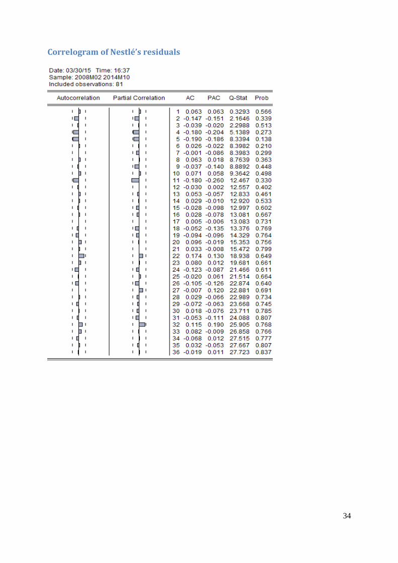
34

Correlogram of Nestlé’s residuals

35

Correlogram of Unilever’s residuals

36

Appendix C. Risk Management Strategies of the Firms This appendix consists of information that could be retrieved from the firms’ websites and financial statements regarding their risks of volatility in raw material prices. Some of the firms have provided more information via email and this has been included in this appendix as well.

Nutreco Nutreco has a portfolio of different products, in an increasing number of different markets and geographies with operations spread over as well mature as emerging markets. As a result, the risks are spread as well. Nutreco is partly exposed to risks arising from fluctuations in market prices. Nutreco aims to minimise the economic risks related to the purchase of raw materials. The business model in animal nutrition and fish feed is largely based on the pass through of raw material prices in selling prices either by virtue of standing industry practice or by virtue of customer contracts. In 2014, Nutreco continued further implementation of its revised Procurement Risk Management Policy, which provides guidance on positions that may be taken regarding raw materials, with differences depending on the nature of the business, and giving clear authorisation levels based on time horizons, coverage in months and financial magnitude. Nutreco’s raw material contract positions are based on a thorough understanding of its business models, the raw material supply markets and contracts with its feed customers. Purchase decisions are taken either centrally, strongly coordinated or locally, depending on the nature of the related supply markets and the characteristics of the business needs. This has resulted in a centrally coordinated approach for the purchasing of many feed ingredients, like vitamins and amino acids, while many agri-commodities are purchased regionally and locally. In the case of regional and local execution, raw materials are purchased within the limits of the Procurement Risk Management Policy. In addition, Nutreco has global teams of purchasing and supply market experts that share knowledge of market developments, suppliers and supply conditions. This enables Nutreco as a whole to achieve good purchase performance, while minimising the financial risks. This means that all Nutreco employees involved in the contracting of materials operate within a framework of centrally specified policies and guidelines and must act in conformance with the required internal control measures. Compliance is monitored by Procurement, BU management and the Executive Committee, supported by Group Internal Audit. Existing contract positions are closely monitored and, when necessary, remediation actions are evaluated and executed. With the rollout of the Unite project, monitoring and reporting of contract positions and related financial exposure is further standardised.

37

Danone The Group’s raw materials needs mainly involve materials for the production of food products and beverages, notably milk and fruit (“food raw materials”). In value, milk represents the leading raw material purchased by the Group. These purchases consist mainly of liquid milk, for which the operating subsidiaries generally enter into supply agreements with local producers or cooperatives. The liquid milk price is set locally, over contractual periods that vary from one country to the next. The main other food raw materials are fruit-based preparations and sugar; Energy raw materials. They represent a limited portion of the Group’s purchases. Price changes for the main raw materials can substantially influence the volatility of the Group’s earnings. In that regard, the Group manages raw materials cost inflation through the following measures, ranked in order of importance:

• continuous improvements to productivity: the Group strives to optimize its use of raw materials (reduced waste, lighter packaging, better use of milk sub-components in its various products), and to take advantage of pooled purchasing for its various subsidiaries. In 2013, for example, the Group established a centralized purchasing unit for the Fresh Dairy Products Division other than milk; • establishment of a purchasing policy ( Market Risk Management ) that consists of defining rules for securing physical supply and price-setting with suppliers and/or in financial markets when they exist. The monitoring of exposures and of the implementation of this policy is handled by the Group’s central buyers for each raw materials category. The buyers typically negotiate forward agreements with suppliers, since no financial markets exist that would make it possible to fully hedge the price volatility of the Group’s main raw materials. Forward purchasing agreements are monitored at the Group level for each annual closing.

Corbion As Corbion has seen in previous years, sudden volatility in the price of their key raw materials can seriously impact the margins of its products sold. Scarcity of raw materials due to excessive demand or production interruption at suppliers can also impact the results due to sales declines and additional costs incurred to meet the raw materials needs. Their procurement organization, globally organized with dedicated finance support, has developed adequate measures to secure contract positions and to obtain financial instruments to minimize or delay exposure to cost fluctuations in raw materials prices that could negatively impact its margins. These measures include early warnings of possible impact to the organization and its customers. Furthermore, they have implemented a multiple-supplier sourcing policy for their most critical raw materials (soy bean oil, sugar, corn, and wheat).. However, climate events, such as droughts, can have a deep impact on their supply costs. they are mitigating those risks actively by taking longer-term contract positions and by approving raw materials from other regions of the world. For sugar, Corbion’s main raw material, they had relatively long price covers at the start of 2013, all against committed sales volumes. On the other key commodities they saw lower raw material costs as a result of the declining markets. Mail contact: Dear Arjan, Unfortunately I can’t help you with many of the questions as much of it is competitively sensitive information. There’s some information in our annual report 2013 at page 19/20, including a rough breakdown of our raw material spend. The annual report 2014 will be published within a few days. Best regards, Jeroen van Harten IR Corbion

38

Unilever Unilever is one of the world's largest Consumer Products (CP) companies and the global market leader in all food categories in which it operates. Unilever selected Triple Point's SAP-endorsed commodity management solution to support the establishment of a Global Commodities Operating Team charged with optimizing raw material procurement. The centralized group will consolidate buying activities across all commodities and business units, allowing Unilever to proactively react to market changes and protect margins. Triple Point's joint commodity management solution with SAP enables Unilever to consolidate commodities procurement within an integrated platform, greatly increasing efficiency and improving risk management capabilities. Triple Point's Commodity SL™ is one of only 22 SAP-Endorsed Business Solutions (EBS) worldwide and the only EBS in the commodity trading and risk management space. Commodity SL pre-integrates with the SAP® ERP application to optimize profits across the commodities supply chain. The tightly integrated software is fully tested by SAP, eliminating the need for custom integration. It also delivers a common maintenance program and technology platform, providing the highest value at the least risk. Commodity SL seamlessly integrates Triple Point's real-time, market-based portfolio and enterprise risk management capability with SAP's advanced logistical and accounting solutions to deliver cutting-edge application functionality and decision support Mail contact: Hello Arjan, In response to your query, we typically have 3-6 months forward cover of raw and packaging materials. In our experience this typically roughly corresponds to the time needed to reflect changes in costs in our selling prices. This helps us manage the risk to our margins. Hope this helps Kind regards, Unilever Investor Relations

39

Nestlé Methods include purchasing their main raw materials directly from more than 680 000 small-scale suppliers in 2011. Its network of 1140 sourcing staff and agronomists and 10 625 support staff offered support, training and technical assistance to the farmers who supply them. These actions are expected to create value for shareholders and society and reduce the magnitude of impact of the risk to low over a 10 years timeframe. Mail contact: Dear Arjan Thanks a lot for your interest in Nestlé. Please find below a link to a presentation we made 3 years ago on procurement. Principles have not changed materially and you will find a detailed answer to your questions (audio is also available). http://www.nestle.com/asset-library/Documents/Library/Presentations/Investors_Events/Investor_seminar_2011/NIS2011-03-Procurement-KPetrie.pdf As a summary, Nestlé works more and more directly with farmers to ensure quality and quantity of raw materials needed (see website on rural farming). Clearly we also make use of forward buying and hedging to limit impact of volatility especially for those traded on stock exchanges such as coffee, cocoa, etc. Cover is not disclosed. Let us know if you need more.

Best Regards,

Luca Borlini Investor Relations Nestlé S.A.

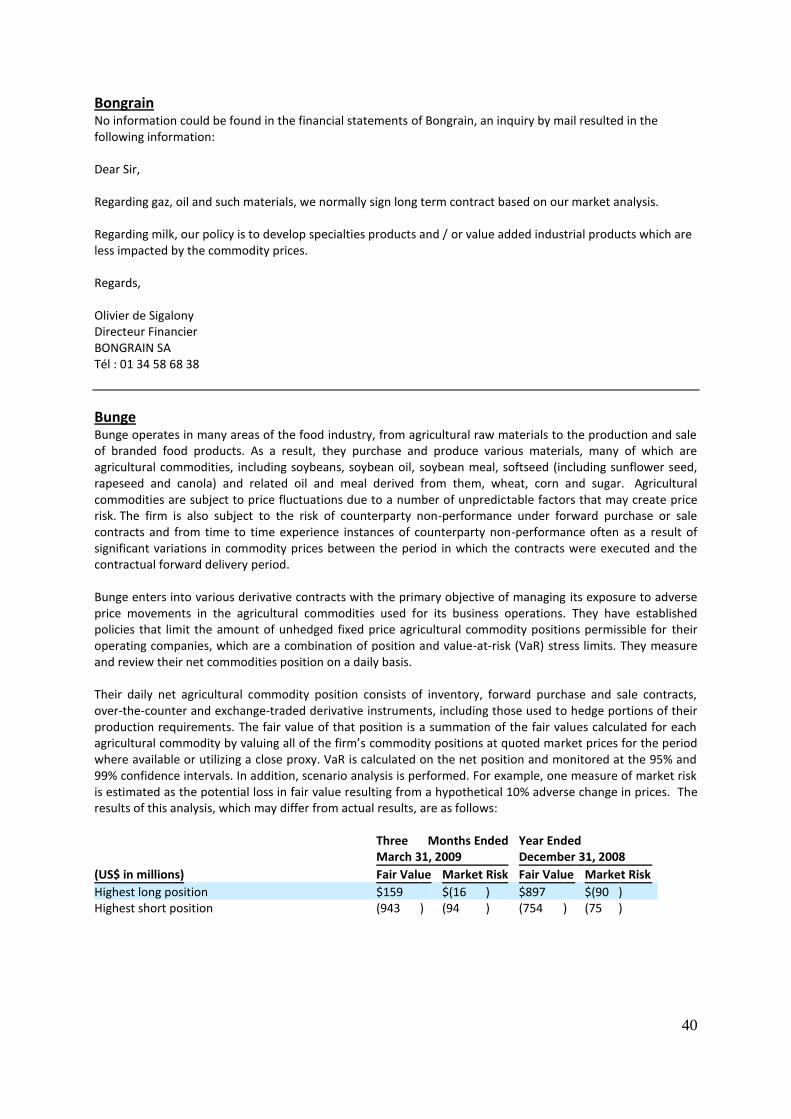
http://www.nestle.com/asset-library/Documents/Library/Presentations/Investors_Events/Investor_seminar_2011/NIS2011-03-Procurement-KPetrie.pdf



40

Bongrain

No information could be found in the financial statements of Bongrain, an inquiry by mail resulted in the following information: Dear Sir, Regarding gaz, oil and such materials, we normally sign long term contract based on our market analysis. Regarding milk, our policy is to develop specialties products and / or value added industrial products which are less impacted by the commodity prices. Regards, Olivier de Sigalony Directeur Financier BONGRAIN SA Tél : 01 34 58 68 38

Bunge Bunge operates in many areas of the food industry, from agricultural raw materials to the production and sale of branded food products. As a result, they purchase and produce various materials, many of which are agricultural commodities, including soybeans, soybean oil, soybean meal, softseed (including sunflower seed, rapeseed and canola) and related oil and meal derived from them, wheat, corn and sugar. Agricultural commodities are subject to price fluctuations due to a number of unpredictable factors that may create price risk. The firm is also subject to the risk of counterparty non-performance under forward purchase or sale contracts and from time to time experience instances of counterparty non-performance often as a result of significant variations in commodity prices between the period in which the contracts were executed and the contractual forward delivery period.

Bunge enters into various derivative contracts with the primary objective of managing its exposure to adverse price movements in the agricultural commodities used for its business operations. They have established policies that limit the amount of unhedged fixed price agricultural commodity positions permissible for their operating companies, which are a combination of position and value-at-risk (VaR) stress limits. They measure and review their net commodities position on a daily basis.

Their daily net agricultural commodity position consists of inventory, forward purchase and sale contracts, over-the-counter and exchange-traded derivative instruments, including those used to hedge portions of their production requirements. The fair value of that position is a summation of the fair values calculated for each agricultural commodity by valuing all of the firm’s commodity positions at quoted market prices for the period where available or utilizing a close proxy. VaR is calculated on the net position and monitored at the 95% and 99% confidence intervals. In addition, scenario analysis is performed. For example, one measure of market risk is estimated as the potential loss in fair value resulting from a hypothetical 10% adverse change in prices. The results of this analysis, which may differ from actual results, are as follows:

Three Months Ended March 31, 2009

Year Ended December 31, 2008

(US$ in millions) Fair Value Market Risk Fair Value Market Risk

Highest long position $159 $(16 ) $897 $(90 ) Highest short position (943 ) (94 ) (754 ) (75 )

41

Appendix D. Results of Augmented Dickey Fuller tests

FIRST Differenced t-Statistic Prob.* -10.51432 0.0000

-3.467205

-2.877636

-2.575430

Null Hypothesis: BARLEY_BRAS has a unit root

Exogenous: Constant Lag Length: 1 (Automatic - based on SIC, maxlag=13) LEVELS t-Statistic Prob.* Augmented Dickey-Fuller test statistic -2.191112 0.2103

Test critical values: 1% level -3.467418

5% level -2.877729

10% level -2.575480

Null Hypothesis: BONGRAIN has a unit root



5% level -2.877544

10% level -2.575381

Null Hypothesis: BUNGEEURO has a unit root

Exogenous: Constant Lag Length: 1 (Automatic - based on SIC, maxlag=13) LEVELS

t-Statistic Prob.* Augmented Dickey-Fuller test statistic -1.439094 0.5618


5% level -2.879610

10% level -2.576484

Null Hypothesis: AEX has a unit root



5% level -2.877636

10% level -2.575430


-3.467418

-2.877729

-2.575480


-3.467205

-2.877636

-2.575430


-3.471719

-2.879610

-2.576484

42

Null Hypothesis: CORBION has a unit root



5% level -2.877544

10% level -2.575381

Null Hypothesis: CRUDEOIL has a unit root




5% level -2.877636

10% level -2.575430

Null Hypothesis: DANONE has a unit root



5% level -2.877636

10% level -2.575430

Null Hypothesis: EGGS has a unit root



5% level -2.877636

10% level -2.575430

FIRST DIFferenced t-Statistic Prob.* -13.70269 0.0000

-3.467205

-2.877636

-2.575430


-3.467205

-2.877636

-2.575430


-3.467205

-2.877636

-2.575430


-3.467205

-2.877636

-2.575430

43

Null Hypothesis: MAIZE has a unit root




5% level -2.877823

10% level -2.575530

Null Hypothesis: MILK has a unit root



5% level -2.878413

10% level -2.575844

Null Hypothesis: NESTLE has a unit root

Exogenous: Constant Lag Length: 0 (Automatic - based on SIC, maxlag=11) LEVELS t-Statistic Prob.* Augmented Dickey-Fuller test statistic 0.713126 0.9918


5% level -2.896779

10% level -2.585626

Null Hypothesis: NUTRECO has a unit root

Exogenous: Constant lag Length: 0 (Automatic - based on SIC, maxlag=13) LEVELS t-Statistic Prob.* Augmented Dickey-Fuller test statistic 1.170310 0.9979


5% level -2.877544

10% level -2.575381

FIRST DIfferenced t-Statistic Prob.* -7.855213 0.0000

-3.467633

-2.877823

-2.575530


-3.467851

-2.877919

-2.575581


-3.512290

-2.897223

-2.585861


-3.467205

-2.877636

-2.575430

44

Null Hypothesis: OATS has a unit root




5% level -2.877729

10% level -2.575480

Null Hypothesis: RICE has a unit root



5% level -2.877729

10% level -2.575480

Null Hypothesis: RYE_PAN has a unit root



5% level -2.877729

10% level -2.575480

Null Hypothesis: SOYBEANS has a unit root




5% level -2.877636

10% level -2.575430


-3.467418

-2.877729

-2.575480


-3.467418

-2.877729

-2.575480


-3.467418

-2.877729

-2.575480


-3.467205

-2.877636

-2.575430

45

Null Hypothesis: SUGAREURO has a unit root




5% level -2.877729

10% level -2.575480

Null Hypothesis: UNILEVER has a unit root

Exogenous: Constant Lag Length: 0 (Automatic - based on SIC, maxlag=12) LEVELS t-Statistic Prob.* Augmented Dickey-Fuller test statistic 0.096652 0.9640


5% level -2.890037

10% level -2.582041

Null Hypothesis: WHEAT_PAN has a unit root



5% level -2.877919

10% level -2.575581


-3.467633

-2.877823

-2.575530


-3.496346

-2.890327

-2.582196


-3.467851

-2.877919

-2.575581

MSc Thesis Chair Group Business Economics Agricultural ...

Documents

Transcript of MSc Thesis Chair Group Business Economics Agricultural ...