MSAT – A new toolkit for the analysis of

elastic and seismic anisotropy 1

Andrew M. Walker a,∗ and James Wookey a

aSchool of Earth Sciences, University of Bristol, Wills Memorial Building, Queen’s

Road, Bristol, BS8 1RJ, UK

Abstract

The design and content of MSAT, a new Matlab toolkit for the study and analysis

of seismic and elastic anisotropy, is described. Along with a brief introduction to the

basic theory of anisotropic elasticity and a guide to the functions provided by the

toolkit, three example applications are discussed. First, the toolkit is used to anal-

yse the effect of pressure on the elasticity of the monoclinic upper mantle mineral

diopside. Second, the degree to which a model of elasticity in the lowermost man-

tle can be approximated by transverse isotropy is examined. Finally backazimuthal

variation in the effective shear wave splitting caused by two anisotropic layers where

the lower layer is dipping is calculated. MSAT can be freely reused for any purpose

and the implementation of these and other examples are distributed with the source

code.

Key words: MATLAB, anisotropy, shear-wave splitting, elasticity, seismology

∗ phone: +44 (0)117 9545245, fax: +44 (0)117 9253385Email addresses: andrew.walker@bristol.ac.uk (Andrew M. Walker),

j.wookey@bristol.ac.uk (James Wookey).1 NOTICE: this is the author’s version of a work that was accepted for publicationin “Computers and Geosciences”. Changes resulting from the publishing process,

Preprint submitted to Elsevier Science 1 October 2012

1 Introduction

The observation and analysis of seismic anisotropy has become a powerful tool

in global, industrial and environmental geophysics with applications as varied

as the study of mantle convection (e.g. Savage, 1999; Panning and Romanow-

icz, 2004; Becker et al., 2012), subduction zones (e.g. Nakajima and Hasegawa,

2004; Morley et al., 2006; Di Leo et al., 2012) and other plate boundaries (e.g.

Kosarin et al., 2011; Lin et al., 2011; Nowacki et al., 2012), continental and

lithospheric structure (e.g. Silver and Chan, 1988, 1991; Bastow et al., 2010,

2011), hydrocarbon exploration and extraction (e.g. Kendall et al., 2007; Win-

terstein et al., 2001; Verdon and Kendall, 2011), and the monitoring of CO2

storage sites (Verdon et al., 2011). Consequences of the anisotropic nature of

the Earth include the splitting of S-waves into two perpendicularly polarised

arrivals with different wave speeds (Crampin, 1984a), the variation in ampli-

tude of reflected (Hall and Kendall, 2000) and converted waves (Vinnik et al.,

2007) with direction, and, most simply, a variation in wave velocity with prop-

agation direction (Hess, 1964). On the length-scales probed by seismology the

anisotropy can arise from a variety of processes. These include the generation

of aligned fractures (Hudson, 1981, 1980; Crampin, 1984b), solid or liquid filled

inclusions (Tandon and Weng, 1984), sedimentary layering (Backus, 1962), or

the alignment of crystals by solid state deformation (e.g. Wenk, 1999), growth

from a melt (e.g. Bergman et al., 2005) or sedimentary deposition (Valcke

et al., 2006). A large amount of information can thus be recovered by measur-

such as peer review, editing, corrections, structural formatting, and other qualitycontrol mechanisms may not be reflected in this document. Changes may havebeen made to this work since it was submitted for publication. A definitive versionwas subsequently published in Computers and Geosciences, [49 pp.81–90 (2012)].http://dx.doi.org/10.1016/j.cageo.2012.05.031

2

ing and modelling the seismic consequences of anisotropy.

Since studies of seismic anisotropy rarely end with its measurement, modelling

tools are needed to provide explanations for its physical origin and to yield

useful geological or geophysical information. Seismic anisotropy reflects an un-

derling anisotropy in the elastic properties of the material through which the

waves propagate. More than two elastic constants (e.g. the bulk and shear

moduli) are needed to describe the relationship between stress and elastic

strain. Indeed, in the most general case 21 distinct elastic moduli are needed

to link the six components of the general stress tensor to the six components

of the strain tensor or to calculate the velocities of seismic waves propagat-

ing through an anisotropic body. This makes software designed to handle

anisotropic elasticity more complex than codes limited to the isotropic case

but the cost of the added complexity can yield significant insight into the

geological problem in hand. Here we describe a new Matlab toolbox, called

MSAT, designed to aid the modelling needed for the interpretative step of

the analysis of seismic anisotropy and to enable studies of elastic anisotropy

more generally. Provision of key building blocks for modelling in this modern

integrated development environment allows the rapid development and pro-

totyping of explanations for measured anisotropy. The Matlab graphical envi-

ronment also permits plotting of key anisotropic parameters. Furthermore, the

software complements SplitLab (Wustefeld et al., 2008) a Matlab environment

used for measuring shear wave splitting and the MTEX toolbox (Bachmann

et al., 2010; Mainprice et al., 2011) used for the analysis of textures in rocks.

The remaining parts of the paper are arranged as follows. In section 2 we re-

view some of the key theoretical and mathematical concepts needed in order

to model seismic and elastic anisotropy. Section 3 contains a description of

3

the design, implementation, availability, capability and contents of the MSAT

toolbox. Three example applications of the software are given in section 4 and

the paper closes with a concise summary and some ideas for further develop-

ment.

2 Background theory

MSAT is concerned with linear elasticity, the continuum theory describing the

relationship between stresses and small, instantaneous and recoverable strains.

As a measure of internal force per-unit area, stress can be represented by a

second rank tensor, σ. Having defined a Cartesian reference frame, a general

stress in three dimensions can be described by three forces, each operating

on the face normal to an axis of the reference frame and, in general, having

three components (one normal to the face and two parallel to it). Denoting the

orientations of the planes and directions of the components of the forces by two

indices, the stress tensor can thus be represented as a nine-element matrix, σij,

which must be symmetric if the body is in equilibrium (is not accelerating).

Strain measures material deformation and this can also be represented by a

second rank tensor, εij = 12(ui,j + uj,i), where u represents a change in length

along an axis and the comma indicates partial differentiation with respect to

direction. This definition also results in a symmetric matrix. The fourth-order

elastic constants (or stiffness) tensor, C, allows the calculation of the stress

required to produce a particular strain:

σij = Cijklεkl, (1)

4

where the repeated indices on the right hand side imply summation in this,

and all similar equations. Similarly, if the stress is known the resulting strain

can be calculated using the compliance tensor which (following the perverse

logic of the stiffness tensor being labelled C) is conventionally denoted S:

εij = Sijklσkl. (2)

MSAT provides a range of functions for analysing and manipulating represen-

tations of elasticity and these are described below (section 3.2). Many of these

contain implementations of different theories, however we will not reproduce

these here: the reader is directed to the works referenced for that background.

However, there are several pieces of theory which underpin several of the func-

tions provided, which are worth covering briefly.

The first of these is the symmetry exhibited by the elastic constants tensor.

The symmetry of the stress and strain tensors implies that Cijkl = Cjikl and

Cijkl = Cijlk (the minor symmetries). Furthermore, it turns out that the

stiffness tensor can be written as a function of the second derivative of the

internal energy, U , with strain:

Cijkl =∂2U

∂εij∂εkl, (3)

and this results in the major symmetries : Cijkl = Cklij. Taken together these

symmetry relations reduce the 81 constants relating 9 stresses to 9 strains to

21 distinct constants relating 6 stresses to 6 strains and these arguments apply

equally to S. For convenience, elastic constants are usually representation using

Voigt notation. This represents the 4th order tensor Cijkl as a symmetric 6×6

5

matrix Cαβ (with no loss of information), where:

ij or kl :

↓ ↓

α β

11 22 33 32 = 23 31 = 13 12 = 21

↓ ↓ ↓ ↓ ↓ ↓

1 2 3 4 5 6

. (4)

It is a convenient property of the Voigt notation C matrix that the equivalent

compliance matrix S can be found by simple matrix inversion. Note, however,

that the compliance matrix cannot be treated quite like the elastic stiffness ,

for example the conversion between the 4th order tensor representation and

the Voigt matrix form includes additional factors for the compliance.

In the most general case discussed above, 21 elastic constants are required to

represent minerals with a triclinic symmetry (such as, for example, albite),

but crystals with a higher symmetry (e.g. orthorhombic, hexagonal or cubic)

require fewer elastic constants. In the simplest case — that of isotropic ma-

terials — this reduces to the two Lame coefficients λ and µ. The reader is

directed to, for example, Babuska and Cara (1991) or Mainprice (2007) for a

detailed discussion of the forms of the elastic matrix for different symmetry

classes. The limitations of what can usually be resolved using seismology mean

that higher symmetry classes are often assumed. A class which is commonly

invoked is transverse isotropy (TI, also known as radial or polar anisotropy,

see, e.g., Thomsen, 1986). In a TI medium properties only vary with angle

from the symmetry axis. This can arise in a number of ways and is exhib-

ited by: crystalline materials with a hexagonal symmetry, isotropic thin layers

of different stiffness (e.g., Backus, 1962), aligned inclusions (e.g., Tandon and

6

Weng, 1984) or cracks which are uniformly oriented (e.g., Hudson, 1980, 1981).

TI requires five independent constants to parameterise. There are a number of

commonly used choices of parameter sets (depending on the area of literature);

MSAT has functions to work with several of these.

The second key piece of background concerns the rotation of elastic constants

tensors. Recall that a vector, v is rotated from to a new orientation, v(R), by

multiplication by a rotation matrix: v(R) = gv, where the rotation matrix, g,

is a 3× 3 orthogonal matrix with determinant 1 and elements that represent

the cosines of angles of the rotation. This transformation be also be written

element-wise as: v(R)i = gijvj (with an implicit summation over j = 1, 3). This

formula can be extended for higher order Cartesian tensors. For example,

the second order stress tensor is rotated: σ(R)ij = gikgjlσkl (with two implicit

summations) and the elastic stiffness tensor rotated: C(R)ijkl = gimgjngkpglqCmnpq

(with four summations and avoiding Voigt notation). For second order tensors

the transformation can also be written in the form of matrix multiplication

by the rotation matrix and its transpose: σ(R) = gσgT , but this shortcut is

not available for higher order tensors. However, it is possible (in fact, highly

desirable for performance reasons) to perform rotations on elastic constants

in Voigt form without requiring to transform to the 3×3×3×3 tensor form. In

order to do this we use the formula from Bond (1943, Equation 8.9):

C(R) = K C KT (5)

where C(R) is the rotated version of C. In this equation K is a 6×6 matrix

derived from combinations of the normal 3×3 rotation matrix and KT is its

matrix transpose. See Bower (2009, Section 3.2.11), Winterstein (1990, page

7

1075) or Bond (1943, Equation 7.2) for details. We note in passing that the

derived matrices for anticlockwise rotation around the principle axes presented

by Bower contain a number of sign errors (a common pitfall when dealing with

rotation matrices!). For reference, the corrected form of these matrices are:

∣∣∣∣∣∣∣∣∣∣∣∣∣∣∣∣∣∣∣∣∣∣∣∣∣∣∣∣∣∣∣∣∣∣∣∣∣

1 0 0 0 0 0

0 c2 s2 −2cs 0 0

0 s2 c2 2cs 0 0

0 cs −cs c2 − s2 0 0

0 0 0 0 c s

0 0 0 0 −s c

∣∣∣∣∣∣∣∣∣∣∣∣∣∣∣∣∣∣∣∣∣∣∣∣∣∣∣∣∣∣∣∣∣∣∣∣∣

∣∣∣∣∣∣∣∣∣∣∣∣∣∣∣∣∣∣∣∣∣∣∣∣∣∣∣∣∣∣∣∣∣∣∣∣∣

c2 0 s2 0 2cs 0

0 1 0 0 0 0

s2 0 c2 0 −2cs 0

0 0 0 c 0 −s

−cs 0 cs 0 c2 − s2 0

0 0 0 s 0 c

∣∣∣∣∣∣∣∣∣∣∣∣∣∣∣∣∣∣∣∣∣∣∣∣∣∣∣∣∣∣∣∣∣∣∣∣∣

∣∣∣∣∣∣∣∣∣∣∣∣∣∣∣∣∣∣∣∣∣∣∣∣∣∣∣∣∣∣∣∣∣∣∣∣∣

c2 s2 0 0 0 −2cs

s2 c2 0 0 0 2cs

0 0 1 0 0 0

0 0 0 c s 0

0 0 0 −s c 0

cs −cs 0 0 0 c2 − s2

∣∣∣∣∣∣∣∣∣∣∣∣∣∣∣∣∣∣∣∣∣∣∣∣∣∣∣∣∣∣∣∣∣∣∣∣∣

(6)

where s = cos θ and c = sin θ, for rotation around the 1-, 2- and 3- axes

respectively. MSAT, however, only uses the general form of the K matrix to

allow arbitrary rotations.

Another technique which underlies many of the routines concerns the averag-

ing of elastic constants. In geophysics we are rarely dealing with single crystals.

We need, therefore, a method of estimating the aggregate elastic properties

of a polycrystalline material containing a range of crystal types and orienta-

tions. While much more rigorous treatments exist (see, e.g., Mainprice, 2007,

for an overview) for many purposes simple averaging schemes suffice. These

either assume constant strain (Voigt averaging) or stress (Reuss averaging)

throughout the sample, and essentially amount to taking the arithmetic aver-

age of each element of the stiffness or compliance tensor, respectively. These

8

two values place an upper (Voigt) and lower (Reuss) bound on the true value.

It was observed by Hill (1952) that experimental values were often close to

the average of these two bounds, a value which has become known as the

Voigt-Reuss-Hill (VRH) average:

CVRH =1

2

(CVoigt + CReuss

)(7)

where

CVoigt =N∑i=1

viCi and CReuss =

[N∑i=1

viSi

]−1

. (8)

Here, vi are the volume fractions of the N individual components, with asso-

ciated elasticities (Ci) and compliances (Si). This is very commonly employed

in geophysics and mineral physics, and is implemented in MS VRH in MSAT.

It should be noted that it is an empirical relation with no strict theoretical

foundation, albeit a useful one.

Finally, MSAT also concerns itself with determining seismic properties from

elastic media. The propagation of motion through an elastic medium is gov-

erned by the elastodynamics equation:

ρ

(∂2ui∂t2

)= Cijkl

(∂2ul∂xjxk

)(9)

where ρ is the density, ui is the displacement, xj is position and t is time. By

substituting into this the displacement associated with a monochromatic plane

wave as a function of time, we obtain the well-known Christoffel equation:

(Cijklnjnl − ρV 2δik

)pk = 0 (10)

where nj is the propagation unit vector, V are the phase velocities, pk are

9

the polarisation unit vectors and δik is the Kronecker delta function. Solutions

to this equation for a given direction (nj) yield the three orthogonal waves

with different phase velocities. One of these will be close to the wavefront

normal (designated quasi-P or qP) and two will be near perpendicular (quasi-

S1, quasi-S2; qS1 and qS2). In practice the quasi- prefix is often omitted.

The reader is directed to Mainprice (2007) for a more complete treatment of

the subject. MSAT follows the methodology of Mainprice (1990) to calculate

phase velocities (see MS phasevels).

3 Software

In order to facilitate the analysis and modelling of observations of seismic

and elastic anisotropy we have developed a new Matlab toolbox, called MSAT

(the Matlab Seismic Anisotropy Toolbox) described below. We chose to write

MSAT in Matlab for a number of reasons including the language’s adoption

by many geophysicists, its portability and the ease of generation of graphical

output. A major strength of Matlab is in the integration of powerful tools for

linear algebra and the manipulation of two-dimensional matrices. We therefore

use the convenient and compact Voigt matrix representation of anisotropic

elasticity and always represent the elasticity as a a rank-two size 6×6 Matlab

array. In the rest of this work and in the MSAT documentation we choose call

these arrays elasticity matrices to avoid confusion with the rank-four elastic

stiffness and elastic compliance tensors.

10

3.1 Design, development and documentation

We developed MSAT using modern tools with ease of use and maintenance in

mind. One important choice involved the way data is represented and func-

tions accessed. Matlab offers facilities for libraries to provide an object oriented

interface — a design which, for MSAT, would imply the creation of elasticity

objects associated with crystals or rocks with functions accessed as methods

belonging to these objects. We chose instead to provide a simple procedu-

ral interface to the library as, in our experience, few seismologists who make

use of Matlab (our target audience) make use of the relatively recent object

oriented facilities offered by the language. In order to avoid some of the dif-

ficulties with namespace ambiguity we impose a common naming convention

and argument ordering to the MSAT functions. All function names begin with

MS and argument lists typically begin with the elasticity matrix followed by

the density.

A second important aspect of usability is accessible documentation. We have

followed the Matlab convention and provide documentation via two routes.

Firstly, the source code of each function contains a comment block describing

what the function does and how it should be used. We have provided this

documentation consistently and always provide key references to the literature

and cross-references to related functions. The Matlab system displays this

documentation in the command window when the built-in help function is

used. The second source of documentation adds a short “getting started”

document, a longer “user guide” and detailed usage examples. These, together

with the function descriptions, are accessible using the Matlab documentation

browser. This documentation is also available on the web. In order to help

11

avoid the situation where documentation and code drift out of sync, we have

built a simple system to create much of this documentation from the comment

blocks in the code. When modifying function behaviour the author (or code

reviewer) only needs to ensure text in the same file as the modified source

code is updated.

In creating MSAT we made use of two modern development tools we consider

essential in order to ease development, future enhancement and maintenance.

We provide a test harness and a set of functionality and regression tests driven

by the xunit toolbox 2 . These tests cover almost all the accessible functions

(except the plotting functions, which are difficult to test automatically) and

provide an easy way to quickly identify the presence of new errors from the

Matlab development environment. We expect new tests will be created to cover

new functionality or to prevent regressions if particular defects are discovered

in the future. In order to allow rapid, independent and parallel development by

multiple authors we made use of git, an advanced distributed version control

system. 3 A web-accessible view of this system, which includes access to the

whole development history, can be accessed online alongside a database to

handle reports of bugs and enhancement requests. 4

3.2 Functions

MSAT provides 27 functions designed to be used together to build tools to

analyse elastic and seismic anisotropy. In describing the basic features of the

2 http://www.mathworks.com/matlabcentral/fileexchange/22846-matlab-xunit-test-framework3 http://git-scm.com/4 https://github.com/andreww/MSAT

12

toolkit we group the functions together according to how elasticity matri-

ces appear in the lists of input or output arguments. In the first group of

functions elasticity matrices are created from the input arguments (Table 1).

MS load and MS load list simply read data from input files (several data for-

mats are supported) while MS elasticDB extracts elasticity information from

a database included with the distribution. Other functions create elasticity

matrices from summary information and a knowledge of the symmetry. For

example, MS iso builds an isotropic elasticity matrix from the P- and S-wave

velocities and density while MS TI creates a matrix with transverse isotropy

and a vertical symmetry axis given, for example, the Thomsen parameters

(Thomsen, 1986).

It is also possible to model the effective anisotropic elasticity caused by partic-

ular rock fabrics; an effect that can be important even if all the components

of the rock are isotropic on a short length scale compared to the seismic

wavelength. For example, if an elastically isotropic medium contains aligned

ellipsoidal inclusions filled with an elastically isotropic material of a different

stiffness the effective elasticity is anisotropic. When the inclusions are axially

symmetric the net effect is the creation of transverse isotropy (Tandon and

Weng, 1984). A similar effect can arise from layering of isotropic materials of

different stiffness (Backus, 1962). This is a common occurrence in sedimen-

tary basins where the beds have distinct lithology and thus elastic properties.

The MS effective medium function allows the creation of elasticity matrices

representing these cases.

The second group of functions include elasticity matrices as input and output.

These functions, listed in Table 2, are used to manipulate or transform an elas-

ticity matrix. Simple examples of these functions are MS rot3, MS rotEuler

13

and MS rotR, which rotate an elasticity matrix (the functions differ in the

way the rotation is specified). MS axes also rotates an input matrix but by an

amount designed to allow the anisotropic nature of the matrix to be analysed.

Such analysis makes use of two other functions, MS decomp and MS norms.

Taken together, these three functions allow the symmetry of elasticity matri-

ces to be expressed following the approach of Browaeys and Chevrot (2004)

and an example of this approach is given below (Section 4.2). Finally, MS VRH

calculates the Voigt, Reuss, and Voigt-Reuss-Hill average elasticity of an ag-

gregate of materials, each described by their own elasticity matrix and volume

fraction, while MS polyaverage takes this averaging one step further and esti-

mates the isotopic elasticity matrix if the components are randomly oriented.

MSAT’s third group of functions (Table 3) allow elasticity to be analysed or

displayed. They take elasticity matrices as input arguments and either re-

turn derived quantities or cause graphics to be produced. Examples include

MS anisotropy, which implements some of the attempts to capture the degree

of elastic anisotropy of a material as a single value (Ledbetter and Miglion,

2006; Ranganathan and Ostoja-Starzewski, 2008) and MS poisson which cal-

culates Poisson’s ratio for a general anisotropic material as a function of di-

rection (Wojciechowski, 2005). MS phasevels solves the Christoffel equation

for given propagation directions and returns the three seismic phase veloc-

ities along with their polarisations. This function is used by MS plot and

MS sphere, which plot the resulting seismic anisotropy on a pole figures and

a three-dimensional spherical representation, respectively (see Section 4.1).

Finally, a few utility functions are also provided (Table 4), which are commonly

used internally by MSAT. These include MS cij2cijkl and MS cijkl2cij,

which convert between Voigt and full tensor notation of elasticity. MS checkC

14

confirms that an elasticity matrix is in the form expected by MSAT and is

physically meaningful.

3.3 Availability

The MSAT code and documentation along with access to key development

tools is available online. 5 The code has been tested using Matlab versions be-

tween 2009b and 2012a but we do not expect issues running on other systems.

MSAT is distributed with a three-clause BSD license and can thus be freely

used, and redistributed, on a commercial or non-commercial basis. We encour-

age users to report any potentially useful changes or enhancements they may

make along with reports of difficulties, bugs and requests for new features.

4 Applications

MSAT can be used for applications in mineral physics and materials science in

addition to seismology. As well as being useful for data analysis and modelling

the toolbox can be used as an aid for rapidly prototyping more involved ap-

plications that will eventually be implemented outside of the Matlab develop-

ment environment. In this section we provide three brief examples of the kind

of applications that MSAT enables. These are chosen to demonstrate usage

for the analysis of single-crystal elasticity data, the calculation and analysis

of the effective elasticity of deformed polycrystalline samples, and modelling

of shear wave splitting. The source code associated with these examples is

distributed along with the toolkit.

5 http://www1.gly.bris.ac.uk/MSAT

15

4.1 Analysis of single crystal elasticity

By themselves, a set of single crystal elastic constants from an experiment or

atomic scale simulation are of limited use to the geophysicist. This is especially

true for low symmetry systems where the link between the elasticity matrix

and properties such as degree of anisotropy or seismic wave speeds can be

disguised by the arithmetic complexity. In this example, we show how MSAT

can be used to illuminate the way that the elasticity of diopside, a monoclinic

upper mantle mineral, changes with pressure. The raw data is derived from

atomic scale calculations making use of density functional theory (Walker,

2012) and covers pressures from 0 to 20 GPa.

The evolution of the individual elastic constants with pressure is shown in

Figure 1 a and b. Whether seen graphically or in a table of numbers one ma-

jor feature stands out: most of the elastic constants increase with increasing

pressure. Careful examination shows that some constants decrease with in-

creasing pressure but without additional computation it is impossible to tell if

the anisotropy increases or decreases or how the pattern of seismic anisotropy

changes. As shown in Listing 1, we can use MSAT to evaluate the degree

of anisotropy as a function of pressure using either the universal anisotropy

index proposed by Ranganathan and Ostoja-Starzewski (2008) or the gen-

eral measure of anisotropy suggested by Ledbetter and Miglion (2006); both

are suitable for monoclinic symmetry. The result, shown in Table 5, is that

pressure has the effect of decreasing the elastic anisotropy of diopside.

The decrease in measures of the overall elastic anisotropy does not necessarily

imply that the observed seismic anisotropy will decreases with pressure. In

16

the mantle a possible mechanism for the generation of seismic anisotropy is

the tendency for the crystal lattices of a material undergoing plastic defor-

mation to align. This leads to the formation of a lattice (or crystallographic)

preferred orientation. The seismic anisotropy as a function of propagation di-

rection through a single crystal becomes interesting as this is the maximum

possible anisotropy that could be generated by this process (e.g. Figure 1 c–e).

Deformed rocks containing diopside often have the diopside crystals aligned

such that the (010) plane is parallel to the shear direction. For horizontal

upper mantle shear and near vertical wave propagation directions (e.g. SKS

phases) it is therefore instructive to consider the shear wave splitting expected

for propagation in the [010] direction in diopside. As shown in Table 5 and

Figure 1 this increases from 5.5% to 19.0% over the 0–20 GPa pressure range,

while the measures of overall anisotropy decrease.

4.2 Polycrystal anisotropy

The lowermost layer of the lower mantle exhibits unusually high seismic anisotropy

(Lay and Young, 1991; Vinnik et al., 1995; Kendall and Silver, 1996; Montag-

ner and Kennett, 1996). Among the explanations for this observation is the

development of a lattice preferred orientation in (Mg,Fe)SiO3 post-perovskite.

If this hypothesis is correct, it offers the possibility of accessing lower-mantle

dynamics from the observation of seismic anisotropy (e.g. Panning and Ro-

manowicz, 2004; Merkel et al., 2007). In an attempt to test this idea, Walker

et al. (2011) simulated the development of post-perovskite LPO in the low-

ermost mantle by combining a tomography-based models of whole mantle

convection (Forte, 2007; Simmons et al., 2007, 2009) with models of polycrys-

17

talline deformation (Lebensohn and Tome, 1993). The initial output of these

simulations are sets of crystal orientations (500 Euler angle triples) at each

sampled point in the lowermost mantle and these were converted into poly-

crystalline elastic constants by forming the Voigt-Reuss-Hill mean of single

crystal post-perovskite elasticity for each orientation (an example of this kind

of calculation is provided with MSAT). In order to compare this elastic model

(which assumes no particular symmetry) with global anisotropic tomography

(Panning and Romanowicz, 2006; Panning et al., 2010; Kustowski et al., 2008),

Walker et al. (2011) then imposed VTI symmetry on the model. In this exam-

ple we show how the appropriateness of this approximation when compared

to the full anisotropic model can be assessed.

The fragment of source code shown in Listing 2 shows one way to assess how

close the general elastic model is to exhibiting hexagonal symmetry. The cal-

culation, which has been repeated for each point in the global model, makes

use of the decomposition method of Browaeys and Chevrot (2004). In MSAT

this is achieved in three steps: first the elasticity matrix is rotated such that

the principle directions of the stress tensor needed to produce an isotropic

dilatation are aligned with the cartesian reference frame. This aligns symme-

try elements with the cartesian frame. Then the (rotated) matrix is projected

onto the orthogonal subspace representing each symmetry class. Finally, the

Euclidean norm of the tensor for each class are calculated. This gives a mea-

sure of the relative contribution of each symmetry class to the initial generally

isotropic tensor (see Browaeys and Chevrot, 2004, for further details). The re-

sults of this analysis are shown in Figure 2 along with the universal anisotropy

index. As can be seen, the proportion of hexagonally is not well correlated with

the overall anisotropy: regions with strongly non-hexagonal anisotropy (red in

18

Figure 2 a) can exhibit both large and small overall anisotropy (Figure 2 b).

However, over the majority of the globe more than 70% of the norm of the

elasticity can be described with an hexagonal approximation.

4.3 Modelling shear wave splitting

Shear-wave splitting is a well known effect of an anisotropic medium on the

passage of a seismic wave through it (Crampin, 1984a). This is the separa-

tion of the shear wave into two orthogonal pulses, the orientation of which

are determined by the medium’s symmetry. These two waves propagate at

different speeds, and so become separated in time. The delay and orientation

of the pulses persist after the wave packet has exited the medium, and can be

measured at the surface in three component seismic data (e.g., Ando et al.,

1980; Vidale, 1986; Silver and Chan, 1988). Shear wave splitting is generally

parameterised by polarisation angle (φ) and the delay time between the two

pulses (δt), sometimes referred to together as the splitting operator (denoted

Γ).

Probably the most common type of study of regional seismic anisotropy analy-

ses shear-wave splitting in SKS/SKKS (core transiting teleseismic shear-wave

phases, e.g., Silver and Chan, 1988, 1991; Savage, 1999). This has been used

extensively to study anisotropy in many tectonic regimes. Other teleseismic

phases (such as S and ScS) have been used extensively to study the deeper

mantle (such as D′′, see Nowacki et al., 2011, for a recent review).

A common situation inferred in SKS/SKKS studies is the presence of multi-

ple layers of anisotropy in the mantle beneath the station. While each layer

19

causes the seismic wave to split, the frequency is generally too low to identify

four individual wave pulses. Instead, an effective splitting is observed (de-

noted ΓEFF) which is a combination of the individual operators and a function

of the initial wave polarisation with respect to the medium fast directions

(e.g., Silver and Savage, 1994). Thus, multiple layers are often inferred from

the presence of a variation of the splitting operator with backazimuth. If lay-

ers also dip, the variation with backazimuth can be highly complex. While

proper waveform modelling is required to completely understand the effects

of complex anisotropy – and more robust modelling inversion methods are

preferable (e.g., Abt and Fischer, 2008; Wookey, 2012) – considerable insight

can be gained from simple models. The MSAT toolset provides methods for

rapidly developing such models for a wide range of circumstances. For exam-

ple, splitting operators for anisotropic models with a range of mechanisms,

orientations and strengths can be calculated with MS phasevels. Multiple op-

erators can then be combined with the equations of Silver and Savage (1994),

implemented in MS effective splitting.

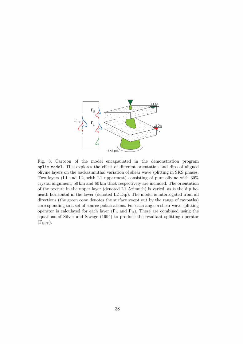
An example of such a model is distributed with the code (split model, see

Listing 3). This uses the aforementioned methods to model the effect of two

layers of aligned olivine on the observation of shear wave splitting in a near-

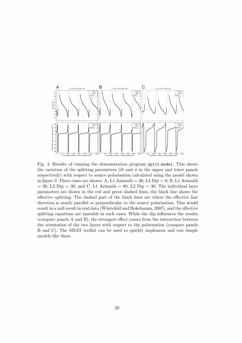
vertically propagating phase (at a slowness similar to SKS). Figure 3 shows

the geometry of the model, and Figure 4 shows the output generated. This

demonstrates the variation of splitting parameters with source polarisation

(which corresponds to backazimuth for SKS which is polarised by its conver-

sion at the core-mantle boundary) for various values of the control parameters

(orientation and dip of the layers). The mild variations of the individual split-

ting parameters associated with each layer combine to predict large effects

20

on the observed effective splitting. While the dip influences the results, the

strongest effect comes from the interaction between the orientation of the two

layers with respect to the polarisation.

5 Summary

We have described a Matlab toolkit designed to simplify the analysis and mod-

elling of elastic and seismic anisotropy. This is fully documented and is freely

reusable on a commercial and non-commercial basis. Notable components in-

clude the consistent implementation of a range of effective medium theories,

tools to rotate, combine, decompose and summarise elasticity matrices, and

functions to calculate parameters relating to seismic wave propagation such as

shear wave splitting. In the examples above we have shown how this toolbox

can be used to analyse single crystal elasticity, the seismic anisotropy of a

polycrystalline aggregate, and backazimuthal variation of shear wave splitting

generated by two dipping layers. Further example applications are distributed

with the toolkit. Potential future enhancements which could be built into new

versions of MSAT include the implementation of additional effective media

theories (e.g. for layers of elastically anisotropic material) or of better approx-

imations of the effect of multiple anisotropic regions along a seismic ray-path.

6 Acknowledgments

We are grateful to a large number of people who have shared code and insight

on elastic and seismic anisotropy over the years, particularly David Mainprice

and Mike Kendall. We also thank colleagues and collaborators who have tested

21

and commented on earlier versions of MSAT. This work has received funding

from the European Research Council under the European Unions Seventh

Framework Programme (FP7/2007-2013) / ERC Grant agreement n◦ 240473

“CoMITAC”.

References

Abt, D. L., Fischer, K. M., 2008. Resolving three-dimensional anisotropic

structure with shear wave splitting tomography. Geophysical Journal In-

ternational 173, 859 – 886.

Ando, M., Ishikawa, Y., Wada, H., 1980. S-wave anisotropy in the upper man-

tle under a volcanic area in Japan. Nature 286, 43 – 46.

Babuska, V., Cara, M., 1991. Seismic Anisotropy in the Earth. Vol. 10 of Mod-

ern Approaches in Geophysics. Kluwer Academic Publishers, Dordrecht,

Netherlands, 224 pp.

Bachmann, F., Hielscher, R., Schaeben, H., 2010. Texture analysis with MTEX

– free and open source software toolbox. Solid State Phenomena 160, 63 –

68.

Backus, G. E., 1962. Long-wave elastic anisotropy produced by horizontal

layering. Journal of Geophysical Research 67, 4427 – 4440.

Bastow, I. D., Pilidou, S., Kendall, J.-M., Stuart, G. W., 2010. Melt-induced

seismic anisotropy and magma assisted rifting in Ethiopia: Evidence from

surface waves. Geochemistry Geophysics Geosystemso 11, Q0AB05.

Bastow, I. D., Thompson, D., Wookey, J., Kendall, J.-M., Helffrich, G., Snyder,

D., Eaton, D., Darbyshire, F. A., 2011. Precambrian plate tectonics: Seismic

evidence from northern Hudson Bay, Canada. Geology 39, 91 – 94.

Becker, T. W., Lebedev, S., Long, M. D., 2012. On the relationship between

22

azimuthal anisotropy from shear wave splitting and surface wave tomogra-

phy. Journal of Geophysical Research 117, B01306.

Bergman, M. I., MacLeod-Silberstein, M., Haskel, M., Chandler, B., Akpan,

N., 2005. A laboratory model for solidification of earth’s core. Physics of

the Earth and Planetary Interiors 153, 150 – 164.

Bond, W. L., 1942. The mathematics of the physical properties of crystals.

The Bell System Technical Journal 22, 1 – 72.

Bower, A. F., 2009. Applied mechanics of solids. CRC Press, Boca Raton,

Florida, USA.

URL http://books.google.co.uk/books?id=1 sCzMNZMEsC

Browaeys, J. T., Chevrot, S., 2004. Decomposition of the elastic tensor and

geophysical applications. Geophysical Journal International 159, 667 – 678.

Chung, D. H., Buessem, W. R., 1967. The Voigt–Reuss–Hill approximation

and elastic moduli of polycrystalline MgO, CaF2, β-ZnS, ZnSe, and DdTe.

Journal of Applied Physics 38, 2535 – 2540.

Cowin, S. C., Mehrabadi, M. M., 1987. On the identification of material sym-

metry for anisotropic elastic materials. Quartely Journal of Mechanics and

Applied Mathematics 40, 451 – 476.

Crampin, S., 1984a. An introduction to wave-propagation in anisotropic me-

dia. Geophysical Journal of the Royal Astronomical Society 76, 17 – 28.

Crampin, S., 1984b. Effective anisotropic elastic constants for wave propaga-

tion through cracked solids. Geophysical Journal of the Royal Astronomical

Society 76, 135 – 145.

Di Leo, J. F., Wookey, J., Hammond, J. O. S., Kendall, J.-M., Kaneshima, S.,

Inoue, H., Yamashina, T., 2012. Deformation and mantle flow beneath the

sangihe subduction zone from seismic anisotropy. Physics of the Earth and

Planetary Interiors 194-195, 38 – 54.

23

Forte, A. M., 2007. Constraints on seismic models from other disciplines –

implications for mantle dynamics and composition. In: Romanowicz, B.,

Dziewonski, A. (Eds.), Treatise on Geophysics. Seismology and the Struc-

ture of the Earth. Vol. 1. Elsevier, pp. 805 – 858.

Hall, S. A., Kendall, J.-M., 2000. Constraining the interpretation of AVOA for

fracture characterisation. In: Ikelle, L., Gangi, A. (Eds.), Anisotropy 2000:

Fractures, Converted Waves, and Case Studies. SEG, pp. 107 – 144.

Hess, H., 1964. Seismic anisotropy of the uppermost mantle under oceans.

Nature 203, 629–631.

Hill, R., 1952. The elastic behaviour of a crystalline aggregate. Proceedings of

the Physics Society A 65, 349 – 354.

Hudson, J. A., 1980. Overall properties of a cracked solid. Mathematical Pro-

ceedings of the Cambridge Philosophical Society 88, 371 – 384.

Hudson, J. A., 1981. Wave speeds and attenuation of elastic waves in material

containing cracks. Geophysical Journal of the Royal Astronomical Society

64, 133 – 150.

Kendall, J.-M., Fisher, Q. J., Covey Crump, S., Maddock, J., Carter, A., Hall,

S. A., Wookey, J., Valcke, S. L. A., Lloyd, G. E., Ben Ismail, W., 2007.

Seismic anisotropy as an indicator of reservoir quality in siliciclastic rocks.

In: Jolley, S. J., Barr, D., Walsh, J. J., Knipe, R. J. (Eds.), Structurally

Complex Reservoirs. Vol. 292 of Special Publication. Geological Society of

London, pp. 123–136.

Kendall, J.-M., Silver, P. G., 1996. Constraints from seismic anisotropy on the

nature of the lowermost mantle. Nature 381, 409 – 412.

Kosarin, M., Davis, P. M., Tanimoto, T., Clayton, R. W., 2011. The rela-

tionship between upper mantle anisotropic structures beneath California,

transpression, and absolute plate motions. Journal of Geophysical Research

24

116, B08307.

Kustowski, B., Ekstrom, G., Dziewonski, 2008. Anisotropic shear-wave veloc-

ity structure of the Earth’s mantle: a global model. Journal of Geophysical

Research 113, B06306.

Lay, T., Young, C. J., 1991. Analysis of seismic SV waves in the core’s penum-

bra. Geophysical Research Letters 18, 1373–1376.

Lebensohn, R. A., Tome, C. N., 1993. A self-consistent anisotropic approach

for the simulation of plastic deformation and texture development of poly-

crystals: Application to zirconium alloys. Acta Metallurgica et Materialia

41 (9), 2611 – 2624.

Ledbetter, H., Miglion, A., 2006. A general elastic-anisotropy measure. Journal

of Applied Physics 100, 063516.

Lin, F.-C., Ritzwoller, M. H., Yang, Y., Moschetti, M. P., Fouch, M. J., 2011.

Complex and variable crustal and uppermost mantle seismic anisotropy in

the western United States. Nature Geoscience 4, 55 – 61.

Love, A. E. H., 1927. A Treatise on the Theory of Elasticity (4th Ed.). Cam-

bridge University Press, Cambridge, UK, 643 pp.

Mainprice, D., 1990. A fortran program to calculate seismic anisotropy from

the lattice preferred orientation of minerals. Computers and Geosciences 16,

385 – 393.

Mainprice, D., 2007. Seismic anisotropy of the deep earth from a mineral and

rock physics perspective. In: Price, G. D. (Ed.), Treatise on Geophysics.

Mineral Physics. Vol. 2. Elsevier, pp. 437 – 491.

Mainprice, D., Hielscher, R., Schaeben, H., 2011. Calculating anisotropic phys-

ical properties from texture data using the MTEX open-source package. In:

Prior, D. J., Rutter, E. H., Tatham, D. J. (Eds.), Deformation Mechanisms,

Rheology and Tectonics: Microstructures, Mechanics and Anisotropy. Vol.

25

360 of Special Publication. The Geological Society of London, pp. 175 – 192.

Merkel, S., McNamara, A. K., Kubo, A., Speziale, S., Miyagi, L., Meng,

Y., Duffy, T. S., Wenk, H.-R., 2007. Deformation of (Mg,Fe)SiO3 post-

perovskite and D” anisotropy. Science 316, 1729 – 1732.

Montagner, J.-P., Kennett, B. L. N., 1996. How to reconcile body-wave and

normal-mode reference Earth models. Geophysical Journal International

125, 229 – 248.

Morley, A. M., Stuart, G. W., Kendall, J.-M., Reyners, M., 2006. Mantle

wedge anisotropy in the Hikurangi subduction zone, central North Island,

New Zealand. Geophysical Research Letters 33, L05301.

Nakajima, J., Hasegawa, A., 2004. Shear-wave polarization anisotropy and

subduction-induced flow in the mantle wedge of northeastern Japan. Earth

and Planetary Science Letters 225, 365 – 377.

Nowacki, A., Kendall, J.-M., Wookey, J., 2012. Mantle anisotropy beneath the

Earth’s mid-ocean ridges. Earth and Planetary Science Letters 317 - 318,

65 – 67.

Nowacki, A., Wookey, J., Kendall, J.-M., 2011. New advances in using seismic

anisotropy, mineral physics and geodynamics to understand deformation in

the lowermost mantle. Journal of Geodynamics 52, 205 – 228.

Panning, M., Romanowicz, B., 2004. Inferences on flow at the base of Earth’s

mantle based on seismic anisotropy. Science 303, 351 – 353.

Panning, M., Romanowicz, B., 2006. A three-dimensional radially anisotropic

model of shear velocity in the whole mantle. Geophysical Journal Interna-

tional 167, 361 – 379.

Panning, M. P., Lekic, V., Romanowicz, B. A., 2010. Importance of crustal

corrections in the development of a new global model of radial anisotropy.

Journal of Geophysical Research 115, B12325.

26

Ranganathan, S. I., Ostoja-Starzewski, M., 2008. Universal elastic anisotropy

index. Physical Review Letters 101, 055504.

Savage, M. K., 1999. Seismic anisotropy and mantle deformation: What have

we learned from shear wave splitting? Reviews of Geophysics 37, 65 – 106.

Silver, P. G., Chan, W. W. J., 1988. Implications for continental structure and

evolution from seismic anisotropy. Nature 335, 34 – 39.

Silver, P. G., Chan, W. W. J., 1991. Shear-wave splitting and subcontinental

mantle deformation. Journal of Geophysical Research 96, 16429 – 16454.

Silver, P. G., Savage, M. K., 1994. The interpretation of shear-wave splitting

parameters in the presence of 2 anisotropic layers. Geophysical Journal In-

ternational 119, 949 – 963.

Simmons, N. A., Forte, A. M., Grand, S. P., 2007. Thermochemical structure

and dynamics of the African superplume. Geophysical Research Letters 34,

L02301.

Simmons, N. A., Forte, A. M., Grand, S. P., 2009. Joint seismic, geodynamic

and mineral physical constraints on three-dimensional mantle heterogeneity:

Implications for the relative importance of thermal versus compositional

heterogeneity. Geophysical Journal International 177, 1284 – 1304.

Tandon, G. P., Weng, G. J., 1984. The effect of aspect ratio of inclusions

on the elastic properties of unidirectionally aligned composites. Polymer

Composites 5, 327 – 333.

Thomsen, L., 1986. Weak elastic anisotropy. Geophysics 51, 1954 – 1966.

Valcke, S. L. A., Casey, M., Lloyd, G. E., Kendall, J.-M., Fisher, Q. J., 2006.

Lattice preferred orientation and seismic anisotropy in sedimentary rocks.

Geophysical Journal International 166, 652 – 666.

Verdon, J. P., Kendall, J.-M., 2011. Detection of multiple fracture sets us-

ing observations of shear-wave splitting in microseismic data. Geophysical

27

Prospecting 59, 593 – 608.

Verdon, J. P., Kendall, J.-M., White, D. J., Angus, D. A., 2011. Linking mi-

croseismic event observations with geomechanical models to minimise the

risks of storing CO2 in geological formations. Earth and Planetary Science

Letters 305, 143 – 152.

Vidale, J. E., 1986. Complex polarization analysis of particle motion. Bulletin

of the Seismological Society of America 76, 1393 – 1405.

Vinnik, L., Romanowicz, B., Le Stunff, Y., Makeyeva, L., 1995. Seismic

anisotropy in the D′′ layer. Geophysical Research Letters 22, 1657 – 1660.

Vinnik, L. P., Aleshin, I. M., Kiselev, S. G., Kosarev, G. L., Makeyeva, L. I.,

2007. Depth localized azimuthal anisotropy from SKS and P receiver func-

tions: The Tien Shan. Geophysical Journal International 169, 1289 – 1299.

Walker, A. M., 2012. The effect of pressure on the elastic properties and seismic

anisotropy of diopside and jadeite from atomic scale simulation. Physics of

the Earth and Planetary Interiors 192-193, 81 – 89.

Walker, A. M., Forte, A. M., Wookey, J., Nowacki, A., Kendall, J.-M., 2011.

Elastic anisotropy of D′′ predicted from global models of mantle flow. Geo-

chemistry Geophysics Geosystems 12, Q10006.

Walker, A. M., Tyer, R. P., Bruin, R. P., Dove, M. T., 2008. The compressibil-

ity and high pressure structure of diopside from first principles simulation.

Physics and Chemistry of Minerals 35, 359 – 366.

Wenk, H.-R., 1999. A voyage through the deformed earth with the self-

consistent model. Modelling and Simulation in Materials Science and Engi-

neering 7, 699 – 722.

Winterstein, D. F., 1990. Velocity anisotropy terminology for geophysics. Geo-

physics 55, 1070 – 1088.

Winterstein, D. F., De, G. S., Meadows, M. A., 2001. Twelve years of vertical

28

birefringence in nine-component VSP data. Geophysics 66, 582 – 597.

Wojciechowski, K. W., 2005. Poisson’s ratio of anisotropic systems. Compu-

tational Methods in Science and Technology 11, 73 – 79.

Wookey, J., 2012. Direct probabilistic inversion of shear-wave data for

anisotropy. Geophysical Journal InternationalIn press.

Wustefeld, A., Bokelmann, G., 2007. Null detection in shear-wave splitting

measurements. Bulletin of the Seismological Society of America 97, 1204 –

1211.

Wustefeld, A., Bokelmann, G., Zaroli, C., Barruol, G., 2008. SplitLab: A shear-

wave splitting environment in Matlab. Computers and Geosciences 34, 515

– 528.

Zenner, C., 1948. Elasticity and Anelasticiy of Metals. University of Chicago

Press.

29

Function name Description and notes

MS build isotropic Create elasticity matrix from pairs of isotropic moduli.

MS TI Generate elastic constants for a vertically transverseisotropic medium from Thomsen parameters (Thomsen,1986), the ξ, φ and η parameters sometimes used inglobal scale tomography (e.g., Panning and Romanow-icz, 2006), or the A,C,F ,L, and N parameters of Love(1927). Symmetry is in the 3-axis in all cases.

MS effective medium Generate elastic constants from various effectivemedium theories. Includes isotropic media containing el-lipsoidal inclusions (Tandon and Weng, 1984), cracked(Hudson, 1980, 1981; Crampin, 1984b) and layered(Backus, 1962) media.

MS elasticDB Database of various elastic constants.

MS expand Fill out an elasticity matrix using symmetry.

MS iso Generate elasticity matrix from isotropic P- and S-wavevelocities and density.

MS load Load an elasticity matrix from a file.

MS load list Load a list of elasticity matrices from a file.

Table 1MSAT functions for the input or generation of elasticity matrices. All return at leastone elasticity matrix

30

Function name Description and notes

MS VRH N-phase Voigt-Reuss-Hill average of elasticity.

MS axes Reorient elasticity matrix for optimal decompositionusing method of Cowin and Mehrabadi (1987) andBrowaeys and Chevrot (2004).

MS decomp Browaeys and Chevrot (2004) decomposition of the elas-ticity matrix.

MS polyaverage Calculate elasticity matrix for an isotropic polycrystalgiven the anisotropic single crystal matrix.

MS rot3 Rotate elasticity matrix around three orthogonal axes.

MS rotEuler Rotate an elasticity matrix given Bunges convention forEuler angles.

MS rotR Use a rotation matrix to rotate an elasticity matrix.

Table 2MSAT functions for the manipulation or transformation of elasticity matrices. Allaccept at least one elasticity matrix as an input argument and return at least onematrix as output.

Function name Description and notes

MS anisotropy Measures of anisotropy defined by Zenner (1948), Chungand Buessem (1967), Ledbetter and Miglion (2006) andRanganathan and Ostoja-Starzewski (2008).

MS norms Browaeys and Chevrot (2004) analysis of the elasticitymatrix.

MS phasevels Calculate wave velocities in anisotropic media (Main-price, 1990).

MS plot Plot wave velocities and anisotropy pole figures.

MS poisson Poisson’s ratio in anisotropic media (Wojciechowski,2005).

MS sphere Plot a spherical plot of wave velocities or anisotropyfrom a set of elastic constants.

Table 3MSAT functions for the analysis and visualisation of elasticity matrices. These func-tions all accept at least one elasticity matrix as input but do not return elasticityas part of the output.

31

Function name Description and notes

MS checkC Check consistency of an elasticity matrix against variouscriteria (must be a positive definite 6 × 6 symmetricMatlab array of real numbers).

MS info Report information about an elasticity matrix.

MS cij2cijkl Convert between an elasticity matrix (Voigt notation)and a rank-four array (full tensor).

MS cijkl2cij Convert a rank-four elasticity tensor (rank-four) to anelasticity matrix (Voigt notation).

MS Vrot3 Rotate a three-vector.

MS rotM Create a rotation matrix.

Table 4MSAT utility functions.

P ρ K G VPiso VSiso AU A? VqS1 VqS2 aVS

GPa kg/m3 GPa GPa km/s km/s - - km/s km/s %

0.0 3276 124.3 71.7 8.4 4.9 0.5 1.9 5.0 4.8 5.5

5.0 3401 147.6 77.8 9.2 5.5 0.4 1.9 5.2 4.9 6.4

10.0 3512 169.2 82.6 9.9 6.1 0.4 1.9 5.4 4.8 11.5

15.0 3612 190.6 88.4 10.5 6.5 0.3 1.8 5.5 4.9 12.4

20.0 3704 208.8 88.7 11.0 7.0 0.3 1.7 5.6 4.6 19.0

Table 5Properties derived from the elasticity of diopside as a function of pressure, P . Thedensity ρ is taken from Walker et al. (2008) while the elastic constants are fromWalker (2012). Calculated derived quantities include: the bulk, K, and shear, G,moduli of isotropic polycrystalline aggregates and their P- and S-wave velocitiesVPiso and VSiso; the universal, AU , and general, A?, anisotropy indices of Ledbetterand Miglion (2006) and Ranganathan and Ostoja-Starzewski (2008), respectively;S-wave velocities, VqS1 and VqS2, and anisotropy, aVS = (VqS1−VqS2)/1

2(VqS1+VqS2),for waves propagating in the [010] direction.

32

1 % Loop over pre s sure s , r ( i ) i s the dens i ty , C( : , : , i )2 % i s the e l a s t i c i t y matrix3 f o r i = 1 : l ength (P)4 % Calcu la te an i so t ropy index5 [ uA, lmA ] = MS anisotropy ( C( : , : , i ) ) ;6 % Calcu la te i s o t r o p i c e l a s t i c i t y7 [ K vrh , G vrh ] = MS polyaverage ( C( : , : , i ) ) ;8 % Get i s o t r o p i c phase v e l o c i t i e s9 Ciso = M S b u i l d i s o t r o p i c ( ’ lam ’ , G vrh , ’K ’ , K vrh ) ;

10 [ ˜ , ˜ , VSiso , ˜ , VPiso ] = MS phasevels ( Ciso , . . .11 r ( i ) , 0 . 0 , 0 . 0 ) ;12 % Calcu la te s p l i t t i n g f o r [ 0 1 0 ] d i r e c t i o n (5km l a y e r )13 % This i s a long the y a x i s .14 [ ˜ , aVS , VS1 , VS2 , ˜ ] = MS phasevels ( C( : , : , i ) , . . .15 r ( i ) , 0 . 0 , 90 .0 ) ;16 dt = (10/VS2 − 10/VS1 ) ;17 % Write r e s u l t s f o r t h i s p r e s su r e18 f p r i n t f ( f o rmat s t r i ng , P( i ) , r ( i ) , K vrh , G vrh , . . .19 VPiso , VSiso , uA, lmA, VS1 , VS2 , aVS ) ;20 end

Listing 1: Part of the source code used to extract anisotropic and seismic pa-rameters from the elasticity of diopside. A full working version of this simpleexample is distributed with MSAT. The elasticity matrix, C(:,:,i) and den-sity, r(i), corresponding to each pressure, P(i) is analysed in turn for degreeof anisotropy (line 5), elasticity of an isotropic aggregate (lines 7-11), andseismic wave speeds and shear-wave splitting magnitude (lines 14-16). Valuesprinted by line 18 are reported in Table 5

33

1 % Rotate to optimum o r i e n t a t i o n2 ChereR = MS axes ( Chere ) ;3 % Decompose in to components4 [ C iso , C hex , C tet , C ort , C mon , C t r i ] = MS decomp( ChereR ) ;5 % Calcu la te norms o f components6 P = MS norms ( ChereR , C iso , C hex , C tet , C ort , C mon , C t r i ) ;7 % Hexagonal as a f r a c t i o n o f t o t a l a n i s o t r o p i c components8 SumA = sum(P( 2 : end ) ) ;9 PercH ( i l a ( i ) , i l o ( i ) ) = P( 2 ) . /SumA ;

Listing 2: Part of the source code used to analyse the lowermost mantle modelshowing how the decomposition approach of Browaeys and Chevrot (2004)is implemented. The elasticity matrix at a point Chere is first rotated toallow optimum decomposition (line 2) then the rotated matrix is decomposedinto isotropic, hexagonal, tetragonal, orthorhombic, monoclinic and tricliniccomponents (line 3). The strength of each component is calculated (line 6; Pis a length 6 array) and the fraction of the total anisotropic component of theelasticity matrix with hexagonal symmetry calculated (lines 8 and 9). A fullworking version of this example is distributed with MSAT and the result ofthis calculation shown in Figure 2 a

34

1 % i n t e r r o g a t e e l a s t i c i t i e s to generate2 % s p l i t t i n g parameters f o r each l a y e r .3 % ( MS phasevels i s v e c t o r i s e d )4 [ pol , ˜ , vs1 , vs2 , ˜ , ˜ , ˜ ] = . . .5 MS phasevels ( L1 C , rh , inc , baz ) ;6 % convert to geog . r e f e r e n c e frame7 f a s t 1 = MS unwind pm 90 ( ( baz − pol ’ ) ) ;8 t l a g 1 = d i s t 1 . / vs2 ’ − d i s t 1 . / vs1 ’ ;9

10 [ pol , ˜ , vs1 , vs2 , ˜ , ˜ , ˜ ] = . . .11 MS phasevels ( L2 C , rh , inc , baz ) ;12 f a s t 2 = MS unwind pm 90 ( ( baz − pol ’ ) ) ;13 t l a g 2 = d i s t 2 . / vs2 ’ − d i s t 2 . / vs1 ’ ;14

15 % Calcu la te the e f f e c t i v e s p l i t t i n g16 % between 2 l a y e r s ( need to loop17 % over propagat ion d i r e c t i o n s )18 f a s t e f f = ze ro s ( s i z e ( baz ) ) ;19 t l a g e f f = f a s t e f f ;20 f o r i = 1 : l ength ( baz )21 [ f a s t e f f ( i ) , t l a g e f f ( i ) ] = . . .22 M S e f f e c t i v e s p l i t t i n g N ( 0 . 1 2 5 , . . .23 baz ( i ) , [ f a s t 2 ( i ) f a s t 1 ( i ) ] , . . .24 [ t l a g 2 ( i ) t l a g 1 ( i ) ] ) ;25 end

Listing 3: Part of the source code used to calculate the effective splittingparameters of the model illustrated in Figure 3. The anisotropic elasticity ofthe two layers is described by L1 C and L2 C and the range of wave propagationdirections is described by two arrays of angles, the back azimuth (baz) and theinclination (inc). Splitting parameters for the two layers are calculated usingMS phasevels (lines 1-13) then combined using MS effective splitting N

(lines 15-25). The remaining portions of the example (not shown) set up thegeometry of the model, the elasticity matrices, and report the model outputin textural and graphical form.

35

Fig. 1. Elasticity and phase velocities of diopside as a function of pressure. Parts(a) and (b) show the evolution of elements of the elasticity matrix with pressureas calculated using density functional theory. (In part (a): squares: C11, unfilledcircles: C22, filled circles: C33 right pointing triangle: C44, left pointing triangle:C55, downwards pointing triangle: C66. In part (b) squares: C12, unfilled circles:C13, filled circles: C23, right pointing triangles: C15, left pointing triangles: C25,downwards pointing triangles: C65, upwards pointing triangles: C43.) Contours inparts (c), (d) and (e) show the variation in the velocity of the qP (left column) anddifference in the velocity of the qS1 and qS2 phases (centre and right column) withpropagation direction (upper hemisphere pole figures created with MS plot withthe cartesian axis system and approximate location of the crystallographic a axisshown in the inset) and pressure. Tick marks in the right hand column indicate thepolarisation direction of the fast shear wave (qS1).

36

Fig. 2. Classifications of models of lowermost mantle anisotropy. Both panels showvariations in properties extracted from a combined flow and texture model of theD′′ (Walker et al., 2011). The upper panel shows the proportion of the predictedanisotropy which is captured by an assumption of vertical transverse isotropy (VTI).The lower panel shows the universal anisotropy index of Ranganathan and Osto-ja-Starzewski (2008). The proportion of hexagonally is not well correlated with theoverall anisotropy. However, over the majority of the globe more than 70% of thenorm of the elasticity can be described with an hexagonal approximation.

37

U

LEFF

L1 Az.

L2 Dip

SKS pol.

Fig. 3. Cartoon of the model encapsulated in the demonstration programsplit model. This explores the effect of different orientation and dips of alignedolivine layers on the backazimuthal variation of shear wave splitting in SKS phases.Two layers (L1 and L2, with L1 uppermost) consisting of pure olivine with 30%crystal alignment, 50 km and 60 km thick respectively are included. The orientationof the texture in the upper layer (denoted L1 Azimuth) is varied, as is the dip be-neath horizontal in the lower (denoted L2 Dip). The model is interrogated from alldirections (the green cone denotes the surface swept out by the range of raypaths)corresponding to a set of source polarisations. For each angle a shear wave splittingoperator is calculated for each layer (ΓL and ΓU). These are combined using theequations of Silver and Savage (1994) to produce the resultant splitting operator(ΓEFF).

38

0.1

0.2

0.3

0.4

0.5

0.6

0.7

0.8

0.9

1

Lag

times

(s)

L1 Az = 30; L2 dip = 00

Upper !Lower !Eff. !

0 50 100 150 200 250 300 350!80

!60

!40

!20

0

20

40

60

80

Polarisation (relative to downdip direction)

Fast

shea

r!wa

ve o

rient

ation

(deg

ree)

Upper !Lower !Eff. !

L1 Az = 30; L2 dip = 30

Upper !Lower !Eff. !

0 50 100 150 200 250 300 350Polarisation (relative to downdip direction)

Upper !Lower !Eff. !

L1 Az = 60; L2 dip = 30

Upper !Lower !Eff. !

0 50 100 150 200 250 300 350Polarisation (relative to downdip direction)

Upper !Lower !Eff. !

A B C

Fig. 4. Results of running the demonstration program split model. This showsthe variation of the splitting parameters (δt and φ in the upper and lower panelsrespectively) with respect to source polarisation calculated using the model shownin figure 3. Three cases are shown: A, L1 Azimuth = 30, L2 Dip = 0; B, L1 Azimuth= 30, L2 Dip = 30; and C, L1 Azimuth = 60, L2 Dip = 30. The individual layerparameters are shown in the red and green dashed lines, the black line shows theeffective splitting. The dashed part of the black lines are where the effective fastdirection is nearly parallel or perpendicular to the source polarisation. This wouldresult in a null result in real data (Wustefeld and Bokelmann, 2007), and the effectivesplitting equations are unstable in such cases. While the dip influences the results(compare panels A and B), the strongest effect comes from the interaction betweenthe orientation of the two layers with respect to the polarisation (compare panelsB and C). The MSAT toolkit can be used to quickly implement and test simplemodels like these.

39