Moving Up the Ladder: The Spatial Determinants of ... Up the Ladder: The Spatial Determinants of...

Moving Up the Ladder: The Spatial Determinants of Intergenerational Occupational Mobility in Rural India

Kunal Sen, Global Development Institute, University of Manchester, Vegard Iversen, Global Development Institute, University of Manchester and Anirudh Krishna, Duke University

Abstract: In this paper, we examine the “geography of mobility” for rural India. We study the

spatial determinants of intergenerational occupational mobility across villages in India.

Using a nationally representative data-set – the Indian Human Development Survey of 2011-

2012, which has detailed information on the occupations of fathers and sons as well as data

on village level covariates, we find clear effects of village level factors in explaining

intergenerational occupational mobility, with remoteness of the village, its agro-ecological

and climactic conditions, infrastructural public goods, and its economic prosperity being

important predictors of whether the son is less likely to follow his parent’s occupation in the

village.

Preliminary. Please do not cite.

1. Introduction

A question of long-standing interest among social scientists is the degree to which an

individual’s status in society is determined by the position of one’s parents. In egalitarian

societies, where you are in the social and economic status ladder should not be principally

determined by your parent’s income, educational level or occupation (Roemer 1998, Bowles

and Gintis 2002). Social mobility research has been concerned with intergenerational

occupational mobility, but much of this research has concentrated on advanced market

economies (Erikson and Goldhorpe 1992, Miles1999). However, this question is of crucial

importance in the developing world, and especially in emerging economies which have

undergone modernisation as they have opened up to the world economy in recent decades.

An emerging literature has studied intergenerational occupational mobility in developing

countries (Lu and Treiman 2007, Krishna 2013, Azam 2015). Much of this literature has

documented the patterns of social mobility both for the general population as well as for

1

certain social groups (Motiram and Singh 2012, Reddy 2015).1 Less understood are what

Chetty et al. (2014) call “the geography of intergenerational mobility” – do we see spatial

variations in intergenerational occupational mobility and if so, what are the spatial

determinants of social mobility in the developing country context?

In this paper, we examine the spatial determinants of intergenerational occupational

mobility across villages in India. The federal nature of India’s polity where local governments

have an important role to play in the provision of local public goods as well as the

systematic differences in agro-ecological conditions, physical infrastructure, human capital,

social structure, economic endowments and the remoteness of villages from centres of

economic activity provide an ideal setting to examine the role of village level factors in

explaining social mobility. We use a nationally representative data set called the Indian

Human Development Survey II which was conducted in 2011-2012 which provides detailed

information on parents and adult age children as well as range of individual and village

characteristics of the location of the adult child. Looking at father-son occupational mobility,

we find find clear effects of village level factors in explaining intergenerational occupational

mobility, with remoteness of the village, its agro-ecological conditions, infrastructural public

goods, and its economic prosperity being important predictors of whether the son is less

likely to follow his parent’s occupation in the village.

The rest of the paper is structured as follows. In the next section, we provide a brief review

of the literature. We then discuss measures of social mobility and describe how we have

categorised the occupations in measuring occupational mobility. We then present the

empirical strategy, followed by the descriptives and the results.

2. Related Literature

1 For example, the literature on India has tended to look at social mobility patterns among different castes in India, and especially the most disadvantaged (see Krishna et al. 2016).

2

A long-standing literature has looked at the spatial determinants of rural poverty in India. In

an important contribution to the literature, Datt and Ravallion (1998) link the changes in

rural poverty (measured alternately by the head-count ratio, the poverty gap, and squared

poverty gap) in a particular State to initial conditions prevailing in the State in 1960 (the

starting date of their analysis), growth in farm output per acre, growth in per capita non-

farm output, changes in the cost of living for agricultural labourers, and per capita state

development expenditure. They show that cross-State variations in trend rate of growth of

average farm yields were important in explaining cross-State variations in the trend rates of

rural poverty reduction.

Palmer-Jones and Sen (2003) have highlighted the role of agro-ecological factors in

mediating the relationship between agricultural growth and rural poverty; they argued that

some Indian States were characterized by relatively homogeneous agro-ecological

properties that were favourable to agricultural growth, and these States, mostly in north-

west India, were provided with appropriate supportive policies (in terms of large-scale

irrigation and access to the new Borlaug seed-fertilizer technology introduced in the mid-

1960s), which accounts in large part for their better performance in terms of both

agricultural growth and poverty reduction, and hence the associations found in State-level

analyses. Other States had very diverse conditions in agro-ecological conditions and these

showed in poorer average performance, even though in some of their regions their

performance is impressive. Thus, while States which experienced rapid agricultural growth

consequently achieved poverty reduction, Palmer-Jones and Sen (2003) show that the

success of these States is due to their possession of a high proportion of favourable agro-

ecological conditions; and where these conditions have not been present, neither poverty

reduction nor agricultural growth has been achieved to the same degree.

Krishna and Bajpai (2011) show that there has been a clear spatial pattern in income growth

in rural India in 1993-2005. While inflation adjusted per capita incomes grew between 1993

and 2004 in villages located within 5 kilometres of the nearest town, they fell in villages

situated more than 5 kilometres of the nearest town (and where more than 80 per cent of

India’s rural population reside). Iversen et al. (2014) find that Scheduled Caste households in

own dominated villages realise higher incomes and far more rapid poverty reduction than

Scheduled Castes living in villages dominated by Upper Castes.

3

Together, these studies show the importance of agro-ecology, remoteness of location and

social structure in being important in explaining spatial patterns in poverty reduction and

income mobility in India. No such study thus far has examined the spatial determinants of

intergenerational occupational mobility. Our study aims to fill this gap.

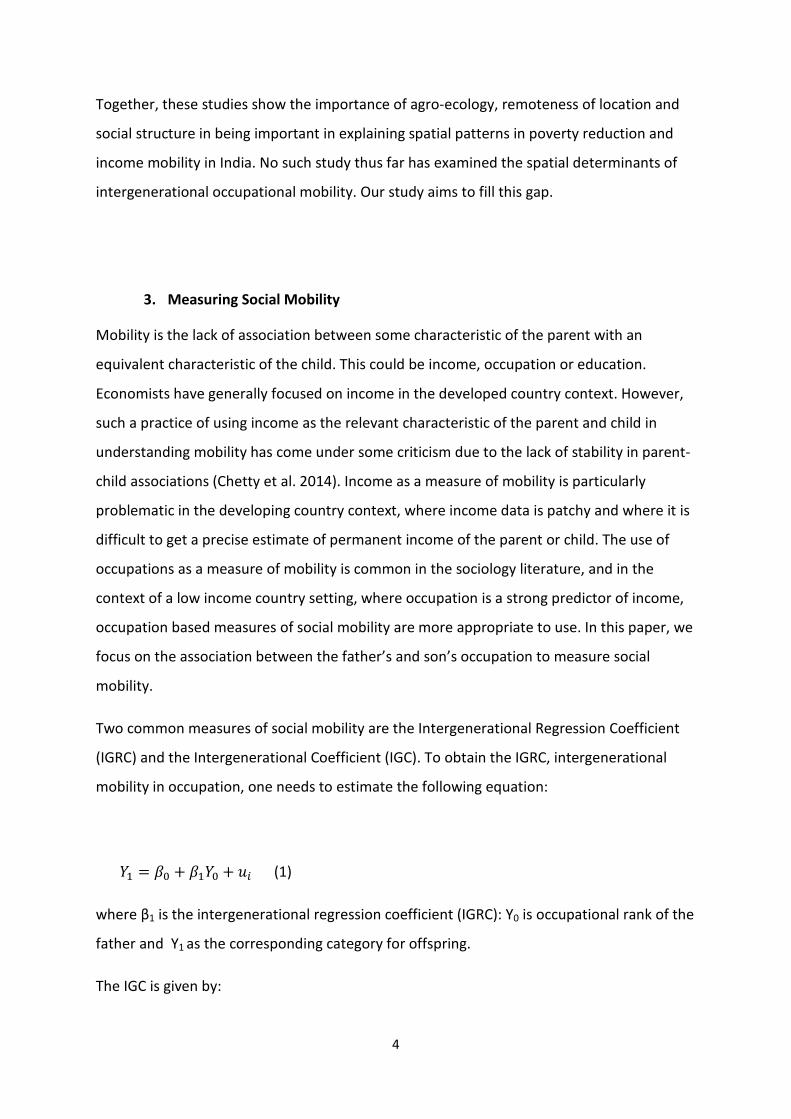
3. Measuring Social Mobility

Mobility is the lack of association between some characteristic of the parent with an

equivalent characteristic of the child. This could be income, occupation or education.

Economists have generally focused on income in the developed country context. However,

such a practice of using income as the relevant characteristic of the parent and child in

understanding mobility has come under some criticism due to the lack of stability in parent-

child associations (Chetty et al. 2014). Income as a measure of mobility is particularly

problematic in the developing country context, where income data is patchy and where it is

difficult to get a precise estimate of permanent income of the parent or child. The use of

occupations as a measure of mobility is common in the sociology literature, and in the

context of a low income country setting, where occupation is a strong predictor of income,

occupation based measures of social mobility are more appropriate to use. In this paper, we

focus on the association between the father’s and son’s occupation to measure social

mobility.

Two common measures of social mobility are the Intergenerational Regression Coefficient

(IGRC) and the Intergenerational Coefficient (IGC). To obtain the IGRC, intergenerational

mobility in occupation, one needs to estimate the following equation:

𝑌𝑌1 = 𝛽𝛽0 + 𝛽𝛽1𝑌𝑌0 + 𝑢𝑢𝑖𝑖 (1)

where β1 is the intergenerational regression coefficient (IGRC): Y0 is occupational rank of the

father and Y1 as the corresponding category for offspring.

The IGC is given by:

4

𝜌𝜌 = 𝛽𝛽1(𝜎𝜎1𝜎𝜎0

) (2)

where σ1 and σ0 are the standard deviations (dispersions) of occupational categories in the

child and parent generation. The social mobility measures in (1) and (2) overlap if the intra-

generational dispersions of occupations are identical for the parent and offspring

generation, which is unlikely. Further, a cross-sectional rise in occupational inequality from

the parent to the child generation will translate into lower social mobility while a relatively

more compressed distribution of occupations in the child generation results in a higher

social mobility estimate (Iversen et al. 2017).

Data

The data is from a large-scale household survey that covers most of the territory of India,

known as the Indian Human Development Survey. We use the 2011-2012 round of the

survey. The survey was carried out by NCAER on behalf of the University of Maryland. An

unique feature of the survey was that the household level questionnaire asked questions to

the heads of the household about his/her parent’s occupation and education. Another

unique feature of the data was that a village level questionnaire was administered to 1420

villages in 384 districts which were asked detailed questions about the physical

infrastructure, agroecological properties, economic conditions and social structure of the

village. One limitation of the survey is that village level GPS coordinates are not released to

researchers as it may compromise the confidentiality of information about the village. This

implies that while we know in which district the village is located, we do not exactly where

in the district the village is located. Furthermore, as the survey was not meant to obtain

representative data at the district or state level, aggregating the data to district or state to

obtain spatial maps of social mobility and village characteristics is not possible.

Categorising Occupations

To estimate the IGRC and IGC, we need a method of categorising occupations such that they

can be rank ordered. The IHDS surveys ask heads of households about the main occupation

of their fathers (or fathers of husbands, if the head of household is female). Since we focus

on father-son occupational mobility, we restrict our sample to male headed households,

5

with heads aged 20 years and above and who are not retired or unfit for work.2 The

occupational codes are provided at the two-digit level (as detailed in the Appendix). In their

analysis of occupational mobility based on IHDS I data, Motiram and Singh (2012) use the

Indian National Classification of Occupations (NCO 2004) which in turn draws on ILO’s

occupational classifications (ISCO88 and its antecedents) with adjustments considered

appropriate for the Indian context (ibid.). A key feature of ISCO88 is the use of skill

requirements as the main principle guiding occupational rank (e.g. Ganzeboom and Treiman

1996). In the Indian context, the translation of skill requirements into occupational status is

made more intricate by caste: independently of the skill requirements of their traditional,

caste-based occupations, Shudra or Scheduled Caste individuals are e.g. likely to have low

social status. We attempt to adjust for this and for other relevant empirical facts when

converting the IHDS categories into an occupational ranking.3 In our analysis, we use the

following six occupational categories (with IHDS occupation codes in brackets).

Table 1: Occupational categories and codes

Category 6 Professional (Occupation codes 00-29) Category 5 Clerical and other (Occupation codes 30-39, 40-49) Category 4 Farmers (Occupation codes 60-62) Category 3 Higher status vocational occupations (Occupation codes 43, 49, 50-52, 56-

59, 79, 84-87). Category 2 Lower status vocational occupations (often caste based, traditional): 53-

55, 68, 71-78, 80-83, 88-93, 96-98) Category 1 Agricultural and other manual laborers including construction workers

(Occupation codes 63-67, 94, 95, 99)

Higher values of the occupational category variable is associated with higher standing on the

social status and plausibly on the earnings ladder. While categories 6 and 5 are quite

straightforward, the placement of farmers as category 4 is less clear cut given the

2 Accordingly, IHDS data are not subject to the coresidence-related selection bias that affects social mobility estimates using NSS data: see e.g. discussions in Azam and Bhatt (2015) and Shahe Emran, Greene and Shilpi (2015). Azam (2015) also includes brothers of the male heads of household residing in the household as well as male children over 20 years whose father is residing in the same household. Including only co-resident brothers and not those who reside somewhere else leads to a problem of selection bias. Including male children whose parents live in the same household has a disadvantage of including sons who may be at a point in their life-cycle where occupational stasus is fluid. 3 We acknowledge the inevitable coarseness and limitations implied by such rankings: an example of another complicating factor in the Indian context is the status distinction between, say, a sweeper in a government job and a sweeper working for a private household.

6

substantive heterogeneity among India’s cultivators.4 For the main questions that we

address and in the tables presented below, this simplification does not represent a major

concern. For the three remaining categories our proposed classification departs, firstly, and

for compelling empirical reasons, from Azam’s (2015), particularly in respect of his granting

construction workers a higher occupational rank than other manual labourers. This is a

major issue since construction represents India’s largest sector of employment outside

agriculture. Among the 30 million plus individuals earning a living in the sector, more than 8

out of 10 are reported to be unskilled and informally employed, often earning an insecure

pittance (NSDC 2010). To classify an occupational change from manual agricultural labour to

construction sector work as upward mobility is therefore problematic. Given the size and

relative importance of this sector, this ordering of occupational categories produces an

upward bias in mobility estimates.

To address caste and occupational status, we distinguish between categories 2 and 3,

capturing low and higher status for a spectrum of vocational and other skills. The idea here

is to distinguish between occupations that are skilled but low status because of a caste

connotation and those that are not: new, modern jobs and vocations form a sub-set of the

latter. Examples of low status vocational occupations (category 2) are blacksmiths and shoe

makers: higher status occupations include tailors while modern vocational occupations

include e.g. machinery/electrical fitters, broadcasting station operators and plumbers.

Finally, and given our focus on sharp ascents we examine whether the lower end layer

within category 6, which we interpret to comprise of nurses (occ code 8) and teachers (occ

code 15), account for a substantive fraction of the entrants into this topmost category. 5

To obtain the occupation codes of sons, we first ascertain whether the head of household is

a farmer: For those individuals who are not farmers, we use the occupational codes

provided in WS4 (for those engaged in wage or salaried work) and in NFIB (for those who

have a primary non-farm business). Clearly, any occupational classification includes an

4 Such cultivator heterogeneity is not unique to India and the challenge this poses is extensively discussed among historians, see e.g Armstrong (1992), Appendix C. 5 We have included teachers and nurses in the highest occupational category, and there may be an argument for including them in the next highest occupational category (clerical and other workers). However, re-classifying the occupational categories by including these two occupations in the next highest category does not result in a substantially different occupational mobility pattern – only 1.5 per cent of fathers and 3.1 of sons were in these two occupations.

7

element of choice and arbitrariness. Employing a different classification schema did not,

however, produce any major changes in the results reported in the following sections.

4. Empirical Strategy

We follow two approaches to assess the spatial correlates of occupational mobility.

The first approach starts off with the workhorse of empirical analysis of intergenerational occupational mobility, as in equation (1) earlier:

𝑌𝑌1 = 𝛽𝛽0 + 𝛽𝛽1𝑌𝑌0 + 𝑢𝑢𝑖𝑖 (3)

where β1 is the intergenerational regression coefficient (IGRC): Y0 is occupational rank of the father and Y1 as the corresponding category for offspring. To see the role of village characteristics on explaining variations in the IGRC spatially, we augment equation (3) with the following specification:

𝑌𝑌1 = 𝛽𝛽0 + 𝛽𝛽1𝑌𝑌0 + 𝛽𝛽2𝑌𝑌0 ∗ 𝑋𝑋 + 𝛽𝛽3𝑍𝑍 + 𝑢𝑢𝑖𝑖 (4)

Where X is a vector of village covariates, X1 to Xn, and Z is a vector of controls.

For a given village characteristic Xi, we can assess whether Xi positively or negative affects

occupational mobility by looking at the sign of β2 . We estimate equations (1) and (2) by

linear probability methods (ordered probit estimates were broadly similar).

Our second approach is to use a multinomial logit to capture individual’s constrained choice

of one occupation over other occupations, which is the standard approach to modelling

occupational choice in the labour economics literature (Abowd and Killingsworth 1984,

Constant and Zimmerman 2003). That is, supposing that s is the occupational choice

(occupational type of the son in our case) variable which takes values of 0, 1, ... , J for J+1

outcomes. The model for determination of s is specified as

∑=

+=== J

jji

jiiij

X

XjsP

1)exp(1

)exp(]Pr[

β

β, (5)

where i indexes the individual and j indexes the choice or outcome.

8

We are specifically interested in upward ascents, and we will examine the role of village

covariates in explaining probability of the son’s mobility to other occupations where the

father is an agricultural or other labourer (the lowest ranked occupation ). The advantage of

the second approach is that we do not need to make an assumption of rank ordering of

occupations, which is the case with the first approach.

Our set of village covariates comes from the previous literature on social mobility as well as

the literature on the spatial determinants of rural poverty and income mobility in India. The

literature on social mobility has identified the role of segregation in reducing social mobility

by reducing exposure to successful peers and role models, decreasing funding for local

public goods such as schools and constraining access to nearby jobs (Wilson 1987, Massey

and Denton 1993, Cutler and Glaeser 1997). Our segmentation variable that is appropriate

in the Indian context is whether social groups in the village live in separate hamlets. The

presence of good quality schools in the area has also been found to be an important

correlate of social mobility (Chetty at al. 2014). We do not have data on the quality of

schools, and in the Indian context, where many villages lack middle and secondary schools,

whether a village has a middle or secondary school is an important marker for the possibility

of human capital formation necessary for social mobility in the village. The presence of

public goods in the village such as access to electricity and a permanent all weather road are

important factors in allowing for income diversification possibilities in the village

(Binswanger et al 1989). Agro-ecological and climactic factors such as the vulnerability of

the village to droughts or flooding limit the possibilities of rural income growth and limits

the variety of jobs in the service sector that may be supported by the village economy

(Palmer-Jones and Sen 2004).Among other geographical factors, the remoteness of the

village from major towns can hinder the possibility of social mobility in the village as

villagers living closer to the towns and cities have opportunities to engage in higher value

activities that serve the needs of the residents of towns and cities which their counterparts

in more remote villages are not able to do (Krishna and Bajpai 2011). Finally, the economic

prosperity of the village is an important predictor of the range of occupations that a village

economy may support. More prosperous villages, whether the prosperity is due to more

productive farming or a flourishing non-agricultural sector, have the incomes to support

higher order occupations in the service and manufacturing sectors.

9

Our set of controls are drawn from the existing literature on social mobility in India. Caste is

an important marker of the possibility of social mobility in rural India, with individuals in

socially disadvantaged social groups such as the Scheduled Castes (SC), Scheduled Tribes

(ST), Other Backward Classes (OBC) exhibit lower rates of social mobility than forward castes

(Iversen et al. 2016). More educated fathers are expected to have sons who are more likely

to to move up the occupational ladder. Finally, we also add state fixed effects to control for

unobserved state-level factors that may be correlated with social mobility.

5. Descriptives

Occupational Mobility Matrices

We begin by providing occupational mobility matrices, first for the combined rural and

urban sample, then separately for the rural and urban samples (Table 2). We note that the

diagonal terms dominate the off-diagonal terms, which suggests that sons in India are likely

to follow the occupations of their fathers. For example, for the all India sample, 58.6 per

cent of the sons of agricultural and other labourers were also in the same occupational

category. Such dominance is not a verdict on India per se, since it tells us little about how

India compares with other countries. Greater upward occupational mobility would be

evident if the off-diagonal elements on the right-hand side of the diagonals dominate the

off-diagonal elements on the left-hand side. We do not find evidence of such mobility,

independent of rural/urban location, and social group.

The matrices point to higher occupational mobility among forward castes than among Other

Backward Classes (OBC) and Scheduled Castes (SC) and Scheduled Tribes (STs) (Table 3).

Among upper castes, we observe sharp ascents for 24.7 percent of the sons of agricultural

and other labourers who enter the highest two occupational categories – clerical and other

workers and professionals. In contrast, in the case of OBC, SC and ST individuals, the

respective numbers are 15.7, 10.6 and 9.3 percent. Also striking and consistent with

Motiram and Singh (2012), we find a much higher prevalence of sharp descents among SC

and ST sons.

10

Table 2. Occupational Mobility Matrices, All India, Rural and Urban Samples (percentages), IHDS II

ALL INDIA, RURAL AND URBAN COMBINED Father’s occupation/Son’s occupation

Agricultural and other labourers

Lower skilled Occupations

Higher skilled Occupations

Farmers

Clerical and other workers

Professionals

Number of observations (n)


58.6 13.6 8.0 5.3 10.1 4.5

10,170 Lower skilled Occupations

14.6 50.0 11.3 2.5 12.8 8.8 3,224

Higher skilled “Occupations

11.5 15.4 42.5 4.0 15.3 11.3 2,311

Farmers 32.2 9.7 7.7 32.4 10.7 7.4 15,500 Clerical and other workers

7.4 12.0 14.7 3.8 48.1 14.0

2,830 Professionals 8.9 9.0 14.1 6.5 23.9 37.6 1,692 RURAL Agricultural and other labourers

67.1 10.8 5.2 6.5 7.3 3.2


24.4 46.5 5.2 6.0 10.8 7.1 1,189


19.7 11.0 40.7 9.6 10.2 8.9 822


15.8 10.5 10.3 10.3 44.3 8.9

719 Professionals 16.3 8.7 9.4 14.9 16.1 34.6 541 URBAN Agricultural and other labourers

33.1 22.3 16.4 1.5 18.5 8.3


7.8 52.5 15.6 0.1 14.2 10.0 2,035


6.6 18.1 43.7 0.6 18.3 12.7 1,489


3.5 12.7 16.8 0.8 49.8 16.4

2,111

11

Professionals 4.7 9.2 16.7 1.7 28.4 39.3 1,151 Note: all observations adjusted by household weights. Figures in rows add up to 100.

Table 3. Occupational Mobility Matrices, By Social Group (percentages), IHDS II

FORWARD CASTE Father’s occupation/Son’s occupation




Farmers


Professionals

Number of observations (n)


43.1 13.9 10.4 7.9 17.6 7.1


7.7 40.9 14.8 3.4 17.5 15.7 693


7.2 15.5 34.9 7.5 19.5 15.6 804


3.5 10.8 13.6 4.0 49.4 18.8

1,330 Professionals 4.3 6.8 11.5 7.2 28.7 41.5 880 OBC Agricultural and other labourers

52.6 15.0 10.3 6.4 10.6 5.1


13.2 51.9 11.5 2.5 13.5 7.5 1,586


9.5 15.5 48.7 1.9 14.7 9.8 1,026


7.7 12.6 16.4 4.5 48.3 10.6

1,050 Professionals 9.4 11.9 17.3 7.5 21.3 32.6 533 SC Agricultural and other labourers

68.4 12.7 5.7 2.6 7.3 3.3


22.7 53.4 7.7 2.5 8.3 5.5 775


25.9 14.6 36.9 3.9 10.5 8.3 366

Farmers 46.4 12.6 7.3 20.7 7.9 5.0 2,266

12


18.6 13.1 13.2 1.7 42.6 10.8

326 Professionals 21.9 10.2 16.3 1.6 18.7 31.4 196 ST6 Agricultural and other labourers

67.5 12.5 3.7 7.1 6.8 2.5


30.4 41.9 9.1 0.2 6.1 12.4 105


20.9 18.0 38.9 6.1 9.2 7.0 75


18.9 10.0 17.4 4.2 34.5 15.2

67 Professionals 24.2 10.0 9.8 8.2 12.1 35.7 50 Note: all observations adjusted by household weights. Figures in rows add up to 100.

Figures 1 to 4 provide a visual depiction of theoccupational mobility matrices. Here we plot

the change in the son’s rank ordered occupation relative to the father’s occupation. We see

quite remarkable descents – where the son’s occupation is often three ranks below the

father’s occupation. This is particularly noticeable for sons from the disadvantaged social

groups.

6 Note that for STs the number of observations in some cells is very small.

13

Figure 1. Father-Son Occupational Change, All Male Heads of Household

Figure 2. Father-Son Occupational Change, SC Male Heads of Household

.3699 .5799

21.5

5.809 5.494

46.22

8.568

5.329

2.489 2.5391.095

010

2030

4050

Per

cent

-5 0 5deltasonocc

.528 .7181

19.68

4.836 4.836

50.39

8.321

4.3931.901 2.64 1.753

010

2030

4050

Per

cent

-5 0 5deltasonocc

14

Figure 3. Father-Son Occupational Change, ST Male Heads of Household

Figure 4. Father-Son Occupational Change, OBC Male Heads of Household

.1881 .2821

33.85

4.043 3.197

44.01

6.629

2.727 2.304 2.069.7052

010

2030

40P

erce

nt

-5 0 5deltasonocc

.3616 .5062

21.53

6.147 5.906

44.47

8.4495.858

2.808 2.8561.109

010

2030

4050

Per

cent

-5 0 5deltasonocc

15

Intergenerational Regression Coefficient (IGRC) and Intergenerational Coefficient (IGC) By District

We now provide estimates of the IGRC and IGC, where we aggregate the village level

observations to the district.7 It is important to note here that the villages in the IHDS are not

representative of the district. So the estimates provided here are not “true” measures of

intergenerational occupational mobility at the district level. Notwithstanding this, we find

clear spatial differences in social mobility across India, as captured by the IGRC and IGC. For

example, Narmada district has an IGRC of 0.001, suggesting that the son’s occupation is very

weakly correlated with the father’s occupation. In contrast, we have the district of Hissar

where the IGRC is 0.84, suggesting very high persistence of parent-son occupation pairs.

7 We drop all estimates where we have les than 20 observations for a particular estimate, as the estimates of IGRC abd IGC would not be reliable in such small samples.

16

Figure 5. Estimates of IGRC and IGC across Districts in India

Village Covariates

We next provide a sense of how different villages are in their physical, economic and social

characteristics in our sample. In Figure 6, we plot the proportion of villages where jatis live

separately, where middle and secondary schools are present, and where there is a pucca

(permanent all weather) road. In 63 per cent of villages, jatis live separately; in 73 per cent

of villages, a middle school is present, in 33 per cent of villages, a secondary school is

present, and in 86 per cent of villages, a pucca road is present. Figure 7 shows that while in

22 per cent of the villages, 100 per cent of households receive electricity, in around one-

third of villages, the proportion of households receiving electricity is 70 per cent or less.

Figure 8 shows distance of the village from the District Headquarters. While 40 per cent of

the villages are located within 30 kilometres of the district headquarters, one-third of the

villages are located 51 kilometres or more from the district headquarters.

-0.2

0

0.2

0.4

0.6

0.8

1

1.2Ba

ram

ula

Sirm

aur

Alm

ora

Fate

haba

dDh

aulp

urJh

alaw

arFa

rruk

abad

Sulta

npur

Mad

huba

niM

arig

aon

Pala

mu

May

urbh

anj

Sona

pur

Raip

urDa

moh

Betu

lJa

mna

gar

Amar

awti

Ahm

adna

gar

Visa

khap

atna

mRa

ichu

rCh

ikm

agal

urPa

lakk

adPe

ram

balu

r

IGRC

IGC

17

Figure 6: Social and Human Capital Characteristics of Villages (per cent)

Figure 7. Village Wise Distribution of Percentage of Households with Electricity

0

10

20

30

40

50

60

70

80

90

100

Where Jatis LiveSeparately

Where MiddleSchool Present

Where SecondarySchool Present

Whether VillageHas Pucca Road

0.0

1.0

2.0

3.0

4.0

5D

ensi

ty

0 20 40 60 80 100Households with Electricity (percentage)

kernel = epanechnikov, bandwidth = 2.6193

18

Figure 8. Distance from District Headquarters (kilometre ranges)

Note: Ranges: 1:<=5 km, 2: 6-10 km, 3: 11-20 km, 4: 21-30 km, 5: >31-50 km, 6: 51-75 km , 7: 76-100 km, 8: >100== km

Agro-ecological conditions also vary significantly across villages. While 53 per cent of villages

have had no drought for the last 7 years, 15 per cent of villages have had droughts for at

least 2 out of the last 7 years (Figure 9). Flooding is less prevalent in the villages in our

sample, with 74 per cent of villages not experiencing flooding in the last 7 years (Figure 10).

Economic prosperity also varies significantly across the sample villages, as is evident from

Figures 11 and 12 in the distribution of mean real agricultural and non-agricultural wages

(nominal agricultural and non-agricultural wages divided by the state poverty line).

Overall, we see striking differences in village infrastructure, schooling endowments, social

segmentation, agro-ecological/climactic conditions and economic prosperity. We now

investigate whether these differences manifest themselves in differential rates of

intergenerational occupational mobility.

0.1

.2.3

Den

sity

0 2 4 6 8Distance from District HQ in Kilometre Ranges

19

Figure 9. Number of Years when the Village has had a Drought in 2006-2012

Figure 10. Number of Years when the Village has had a Flood in 2006-2012

0.1

.2.3

.4.5

Den

sity

0 2 4 6 8Number of Years when Village had a Drought in 2006-2012

0.2

.4.6

.8D

ensi

ty

0 2 4 6 8Number of Years when Village had a Flood in 2006-2012

20

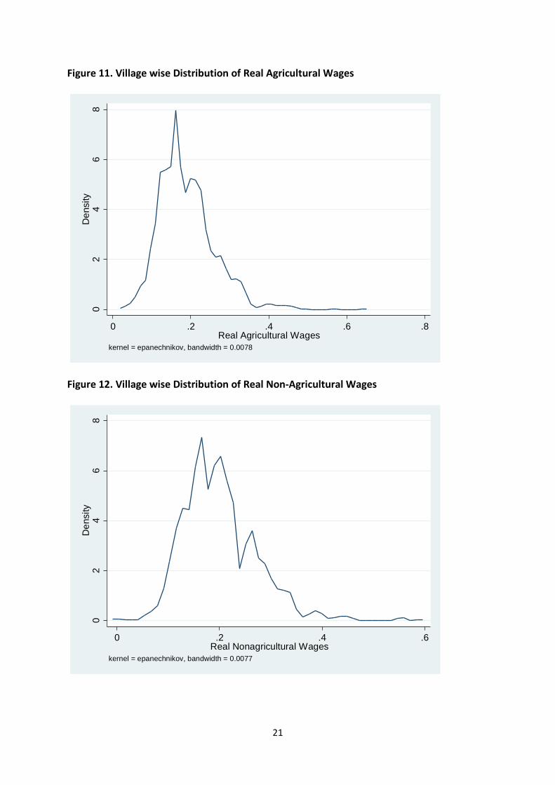
Figure 11. Village wise Distribution of Real Agricultural Wages

Figure 12. Village wise Distribution of Real Non-Agricultural Wages

02

46

8D

ensi

ty

0 .2 .4 .6 .8Real Agricultural Wages


02

46

8D

ensi

ty

0 .2 .4 .6Real Nonagricultural Wages


21

6. Results

We first present estimates of the IGRC augmented with individual level and village level

covariates in Table 3, followed by the multinomial logit estimates of son’s occupational

structure in the case of parents who were agricultural labourers in Table 4. In Col (1) of

Table 4, we present estimates of the IGRC without interacting the father’s occupational rank

with village covariates. In Col. (2), we interact the father’s occupational rank with all village

characteristics. In Col. (3), we add individual level controls – these are the caste status of the

son (SC, ST, OBC), father’s education (in years of education) and the age of the son. Finally in

Col. (4), we include state fixed effects.

We find that remoteness of the village (as captured by the distance from the district

headquarters), agro-ecological conditions of the village – whether the village has been

repeatedly affected by drought and floods, access of the village to the outside world

(captured by the availability of a permanent (pucca) road), and economic conditions of the

village (captured by real agricultural and non-agricultural wages) are important in explaining

intergenerational occupational mobility in all the estimates – the coefficients for these

variables are significant at the 10 per cent or less in Cols (1) to (4). The greater the

remoteness of the village and the larger the number of years that a particular has been

affected by droughts or floods, the lower the mobility of sons relative to fathers (or lessens

the persistence of occupations from fathers to sons). On the other hand, access to a

permanent road and higher real agricultural and non-agricultural wages increases the

mobility of sons relative to fathers in the village. This may reflect the possibility of sons able

to access higher income opportunities in these villages and consequently, move out of

occupations at the lower end of the scale.

Village characteristics that are significant in some specifications but not in all estimates are

whether the village has a secondary school and the percentage of households in the village

with electricity. However, these characteristics are significant in Col. (4), where we include

all individual level controls and state fixed effects. Whether a village has access to a

secondary school and whether households in the village have access to electricity has a

22

positive effect on intergenerational mobility. On the other hand, whether households live in

separate clusters (jatis) or whether the village has a middle school does not seem to affect

social mobility.

With respect to the individual level controls, we obtain the expected results – SC, ST and

OBC male heads are likely to have lower ranked occupations, and father’s education and the

son’s age has a positive effect on social mobility (the latter capturing life-cycle effects).

Finally, in Table 4, we present multinomial logit estimates when the father’s occupation is

an agricultural or other labourer. We want to see to what extent village characteristics

explain the likelihood that the son will move on to higher order occupations, and in

particular, occupations at the top of the social ladder such as clerical workers and

professionals. The relative risk ratios presented in the table capture the effects of village

characteristics on the likelihood of individuals being in other occupational categories elative

to the base category – agricultural/other labourer. We find that social segmentation in the

village (that is, whether jatis stay in separate hamlets) decreases the likelihood that the son

will move into other higher order occupations (except the move to being a farmer).

Remoteness of the village also decreases the likelihood that the son will move into other

higher order occupations (again, except the move to being a farmer). In fact, the nearness

of the village to the district headquarters is the only village characteristic that increases the

likelihood of a sharp ascent – that is, whether an agricultural labourer’s son becomes a

professional. Whether the village has a pucca road decreases the likelihood of an

agricultural labourer’s son being a farmer relative to remaining an agricultural labourer,

while the presence of a middle school increases this likelihood. Higher real non-agricultural

wages has a very strong positive effect on the likelihood of transition from to other

occupations, especially more valued occupations such as clerical workers. In villages with a

flourishing non-agricultural sector, a wider set of occupational possibilities would be

available to the poorer households in the village, including well paid service sector jobs.

23

Our results with the multinomial logit models differ somewhat from the IGRC estimates, and

this may be due to the limitations of the IGRC in capturing mobility patterns among the

households at the bottom of the occupational ladder. While the augmented IGRC estimates

have an intuitive simplicity about them, the multinomial logit approach may be the way

forward to capture more complex mobility patterns (where mobility may be both upward or

downward), and not to make the restrictive assumption of rank ordering of occupations.

24

Table 3. Regression Results, Augmented IGRC Estimates

(1) (2) (3) (4) Intercept 1.49***

(0.025) 1.42*** (0.045)

0.89*** (0.062)

1.11*** (0.126)

IGRC 0.35*** (0.008)

0.28*** (0.058)

0.19*** (0.024)

0.15*** (0.028)

SC -- -- -0.70*** (0.037)

-0.69*** (0.038)

ST -- -- -0.64*** (0.047)

-0.61*** (0.049)

OBC -- -- -0.29*** (0.032)

-0.26*** (0.034)

Father’s Education (in Years)

-- -- 0.07*** (0.004)

0.07*** (0.004)

Age of Son -- -- 0.02*** (0.001)

0.02*** (0.001)

Jatis Stay in Separate Hamlets

-- 0.01 (0.007)

0.003 (0.008)

0.01 (0.008)

Whether Village Has Middle School

-- 0.01 (0.009)

0.02 (0.009)

0.01 (0.009)

Whether Village Has Secondary School

-- 0.02* (0.009)

0.01 (0.009)

0.02* (0.009)

Per cent Households having Electricity

-- 0.001*** (0.0001)

0.0002 (0.0001)

0.001*** (0.0001)

Distance to District HQ (in km ranges)

-- -0.02*** (0.002)

-0.02*** (0.0007)

-0.01*** (0.002)

Number of Years which Village has a Drought in 2006-2012

-- -0.02*** (0.003)

-0.01*** (0.003)

-0.01*** (0.003)

Number of Years which Village has a Flood in 2006-2012

-- -0.01* (0..003)

-0.01** (0.003)

-0.01** (0.003)

Whether Village Has Pucca Road

-- 0.03*** (0.011)

0.03*** (0..011)

0.02* (0..011)

Real Agricultural Wages

-- 0.51*** (0.073)

0.0004*** (0.0007)

0.0003*** (0.0008)

Real Non-agricultural Wages

-- 0.32*** (0.069)

0.0003*** (0.0001)

0.0002** (0.0001)

Number of Observations

20,005 15214 15214 15124

With State Fixed Effects

No No No Yes

Adjusted R square 0.10 0.12 0.19 0.20 Notes: standard errors in parentheses, ***,** and *: significant at 1, 5 and 10 per cent level. Cols (1) and (2) for all individuals, Cols (3) and (4) for SC individuals.

25

Table 5. Multinomial Logit Regressions, Relative Risk Ratios, where the Father is a Labourer

Base Category: Agricultural and Other Labourers

Son’s Occupation


Higher Skilled Occupations

Farmers Clerical Workers Professionals

Jatis Stay in Separate Hamlets

0.80** (-2.24)

0.70*** (-2.90)

0.82 (-1.52)

0.76*** (-2.30)

0.63*** (-2.90)

Whether Village Has Middle School

1.16 (1.11)

1.02 (0.17)

1.35* (1.84)

1.12 (0.76)

1.08 (0.35)

Whether Village Has Secondary School

1.32 (2.48)

1.28 (0.18)

0.81 (-1.35)

1.01 (0.10)

1.34 (0.18(

Per cent Households having Electricity

1.00 (0.03)

1.01*** (2.81)

1.00 (1.41)

0.99 (-1.13)

1.01 (1.24)

Distance to District HQ (in km ranges)

0.86** (-5.02)

0.83*** (-4.93)

0.97 (-0.79)

0.89*** (-3.25)

0.90** (-2.11)

Number of Years which Village has a Drought in 2006-2012

1.04 (0.93)

0.95 (-1.09)

1.06 (1.41)

0.99 (-0.12)

0.99 (-0.23)

Number of Years which Village has a Flood in 2006-2012

0.95 (-1.04)

1.02 (0.40)

0.94 (-0.95)

1.02 (0.404

1.06 (0.87)

Whether Village Has Pucca Road

0.99 (-0.08)

0.88 (-0.65)

0.48*** (-4.41)

1.24 (1.05)

0.95 (-0.31)

Real Agricultural Wages

2.43 (1.06)

1.50 (0.40)

0.07** (-2.21)

0.33 (-1.06)

0.54 (-0.44)

Real Non-agricultural Wages

1.05 (0.07

9.97** (2.54)

9.54* (2.16)

15.57*** (3.07)

0.94 (-0.05)

No of Observations

4904

26

Pseudo- 0.017 Notes: z statistics in parentheses, ***,** and *: significant at 1, 5 and 10 per cent level.

7. Concluding Remarks In this paper, we examined the spatial determinants of intergenerational

occupational mobility in rural India. As has already observed in the literature on

the spatial determinants of rural poverty and income mobility, we have found

clear evidence of the crucial role that geographical factors such as agroecology

and remoteness in explaining social mobility patterns in village India. Physical

infrastructure such as access to roads and electricity also play key roles.

Economic prosperity of the village has a very strong positive effect on social

mobility possibilities. For sons whose parents are agricultural labourers, social

segmentation also plays an important role.

An important limitation of the data that we have used in the paper is that we are

only able to assess intergenerational mobility for sons who have remained in the

village, and not for those who have migrated to cities (or for that matter, to

other villages) since the data on migrants in the surveyed households in the

villages is patchy. The non-inclusion of individuals who have left the village leads

to a selection bias in the estimates of social mobility that we have presented in

the paper. It is difficult to say a priori in which direction the bias manifests itself –

it could be that the individuals who have left the village have a better

occupational profile than those who remained (for example, they have moved to

being clerical workers or professionals in the cities). So we are under-estimating

the effect of village covariates on social mobility. Or it could be that they have

moved to equivalent jobs in the occupational ladder in cities – for example, an

agricultural labourer’s son may have become a construction worker. In this case,

we are over-estimating the effect of village covariates on social mobility. While

interpreting our results, this limitation of the analysis should be kept in mind.

27

References (incomplete)

Armstrong, W. A. (1972). The use of information about occupation, in E. A. Wrigley (ed.): Nineteenth Century Society, Cambridge: Cambridge University Press, pp. 191-310. Azam, Mehtabul (2015). ‘Intergenerational Occupational Mobility among Men in India,” Journal of Development Studies, 51:10, 1389-1408.

Black, Sandra E. and Paul Devereux (2010). “Recent Developments in Intergenerational Mobility,” NBER Working Paper 15889.

Bowles, Samuel and Herbert Gintis (2002). “The Inheritance of Inequality,” Journal of Economic Perspectives, 16 (3): 3-30.

Chetty, Raj, Nathaniel Hendren, Patrick Cline and Emmanuel Saez (2014). ‘Where is the Land of Opportunity? The Geography of Intergenerational Mobility in the United States’, Quarterly Journal of Economics.

Deshpande, Rajeshwari and Suhas Palshikar (2008). “Occupational Mobility: How Much does Caste Matter?,” Economic and Political Weekly, August 23, pp. 61-70.

Erikson, Robert and John H. Goldthorpe (1992). The Constant Flux: A Study of Class Mobility in Industrial Societies. Oxford: Clarendon Press.

Gang, Ira N., Kunal Sen, and Myeong-Su Yun (2016). “Is Caste Destiny? Occupational Diversification among Dalits in Rural India,” European Journal of Development Research, forthcoming.

Ganzeboom, Harry G. and Donald J. Treiman (1996Internationally Comparable Measures of Occupational Status for the 1988 International Standard Classification of Occupations,” Social Science Research, 25(3): 201-39.

Hnatkovska, Viktoria, Amartya Lahiri, and Sourabh B. Paul. (2013). “Breaking the Caste Barrier: Intergenerational Mobility in India,” Journal of Human Resources, 48 (2): 435-73.

Iversen, Vegard, Adriaan Kalwij, Arjan Verschoor and Amaresh Dubey (2014). “Caste Dominance and Economic Performance in Rural India,” Economic Development and Cultural Change, 62(3): 423-57.

Krishna, Anirudh and Devendra Bajpai (2011), “Lineal Spread and Radial Dissipation: Experiencing Growth in Rural India”, Economic and Political Weekly, Sept 17, Vol. XLVI, No. 38,pp. 44-51.

Krishna, Anirudh (2013). “Making it in India: Examining Social Mobility in Three Walks of Life,” Economic and Political Weekly,

Krishna, Anirudh (2013a). “The Spatial Dimension of Inter-Generational Education Achievement in Rural India,” Indian Journal of Human Development, 6 (2): 245-66.

28

Kumar, Sanjay, Anthony Heath and Oliver Heath (2002a). “Determinants of Social Mobility in India,” Economic and Political Weekly, 37 (29): 2983-87.

Kumar, Sanjay, Anthony Heath, and Oliver Heath. (2002b). “Changing Patterns of Social Mobility: Some Trends over Time,” Economic and Political Weekly, October 5, pp. 4091-6.

Majumder, Rajarshee (2010). “Inter-generational Mobility in Educational and Occupational Attainment: A Comparative Study of Social Classes in India,” Margin—The Journal of Applied Economic Research, Vol. 4, No. 4, pp. 463-94.

Miles, Andrew (1999). Social Mobility in Nineteenth – and Early Twentieth Century England, New York: St Martin’s Press.

Motiram, Sripad and Ashish Singh (2012). “How Close Does the Apple Fall to the Tree? Some Evidence on Inter-generational Occupational Mobility in India,” Economic and Political Weekly, 47 (40): 56-65.

OECD (2010). A Family Affair: Intergenerational Social Mobility across OECD Countries. Available at http://www.oecd.org/dataoecd/2/7/45002641.pdf

Perlman, Janice (2011). Favela: Four Decades of Living on the Edge in Rio de Janeiro. Oxford, UK: Oxford University Press.

Reddy, A. Bheemeshwar (2015). “Changes in Intergenerational Occupational Mobility in India: Evidence from National Sample Surveys, 1983–2012.” World Development (76): 329–43

Roemer, John E. (1998). Equality of Opportunity. Cambridge, MA: Harvard University Press.

Shahe Emran, M., W. Greene and F. Shilpi (2016): When Measure Matters: Coresidency, Truncation Bias, and Intergenerational Mobility in Developing Countries, World Bank Policy Research Working Paper No 7608. Wu, Xiaogang and Donald J. Treiman (2007). "Inequality and equality under Chinese socialism: the Hukou system and intergenerational occupational mobility," American Journal of Sociology, 113(2): 415-45.

29

http://www.oecd.org/dataoecd/2/7/45002641.pdf

APPENDIX 1: OCCUPATION CODES

PROFESSIONAL, TECHNICAL AND RELATED WORKERS 00 Physical Scientists 01 Physical Science Technicians 02 Architects, Engineers, Technologists and Surveyors 03 Engineering Technicians 04 Aircraft and Ships Officers 05 Life Scientists 06 Life Science Technicians 07 Physicians and Surgeons (Allopathic Dental and Veterinary Surgeons) 08 Nursing and other Medical and Health Technicians 09 Scientific, Medical and Technical Persons, Other 10 Mathematicians, Statisticians and Related Workers 11 Economists and Related Workers 12 Accountants, Auditors and Related Workers 13 Social Scientists and Related Workers 14 Jurists 15 Teachers 16 Poets, Authors, Journalists and Related Workers 17 Sculptors, Painters, Photographers and Related Creative Artists 18 Composers and Performing Artists 19 Professional Workers, n.e.c. ADMINISTRATIVE, EXECUTIVE AND MANAGERIAL WORKERS 20 Elected and Legislative Officials 21 Administrative and Executive Officials Government and Local Bodies 22 Working Proprietors, Directors and Managers,Wholesale and Retail Trade 23 Directors and Managers, Financial Institutions 24 Working Proprietors, Directors and Managers Mining, Construction, Manufacturing and Related Concerns 25 Working Proprietors, Directors, Managers and Related Executives, Transport, Storage and Communication 26 Working Proprietors, Directors and Managers, Other Service 29 Administrative, Executive and Managerial Workers, n.e.c. CLERICAL AND RELATED WORKERS 30 Clerical and Other Supervisors 31 Village Officials 32 Stenographers, Typists and Card and Tape Punching Operators 33 Book-keepers, Cashiers and Related Workers 34 Computing Machine Operators 35 Clerical and Related Workers, n.e.c. 36 Transport and Communication Supervisors 37 Transport Conductors and Guards 38 Mail Distributors and Related Workers 39 Telephone and Telegraph Operators SALES WORKERS 40 Merchants and Shopkeepers, Wholesale and Retail Trade 41 Manufacturers, Agents 42 Technical Salesmen and Commercial Travellers 43 Salesmen, Shop Assistants and Related Workers 44 Insurance, Real Estate, Securities and Business Service Salesmen and Auctioneers 45 Money Lenders and Pawn Brokers 49 Sales Workers, n.e.c.

30

SERVICE WORKERS 50 Hotel and Restaurant Keepers 51 House Keepers, Matron and Stewards (Domestic and Institutional) 52 Cooks, Waiters, Bartenders and Related Worker (Domestic and Institutional) 53 Maids and Other House Keeping Service Workers n.e.c. 54 Building Caretakers, Sweepers, Cleaners and Related Workers 55 Launderers, Dry-cleaners and Pressers 56 Hair Dressers, Barbers, Beauticians and Related Workers 57 Protective Service Workers 59 Service Workers, n.e.c. FARMERS, FISHERMEN, HUNTERS, LOGGERS AND RELATED WORKERS 60 Farm Plantation, Dairy and Other Managers and Supervisors 61 Cultivators 62 Farmers other than Cultivators 63 Agricultural Labourers 64 Plantation Labourers and Related Workers 65 Other Farm Workers 66 Forestry Workers 67 Hunters and Related Workers 68 Fishermen and Related Workers PRODUCTION AND RELATED WORKERS, TRANSPORT EQUIPMENT OPERATORS AND LABOURERS 71 Miners, Quarrymen, Well Drillers and Related Workers 72 Metal Processors 73 Wood Preparation Workers and Paper Makers 74 Chemical Processors and Related Workers 75 Spinners, Weavers, Knitters, Dyers and Related Workers 76 Tanners, Fellmongers and Pelt Dressers 77 Food and Beverage Processors 78 Tobacco Preparers and Tobacco Product Makers 79 Tailors, Dress Makers, Sewers, Upholsterers and Related Workers 80 Shoe makers and Leather Goods Makers 81 Carpenters, Cabinet and Related Wood Workers 82 Stone Cutters and Carvers 83 Blacksmiths, Tool Makers and Machine Tool Operators 84 Machinery Fitters, Machine Assemblers and Precision Instrument Makers (except Electrical) 85 Electrical Fitters and Related Electrical and Electronic Workers 86 Broadcasting Station and Sound Equipment Operators and Cinema Projectionists 87 Plumbers, Welders, Sheet Metal and Structural Metal Preparers and Erectors 88 Jewellery and Precious Metal Workers and Metal Engravers (Except Printing) 89 Glass Formers, Potters and Related Workers 90 Rubber and Plastic Product Makers 91 Paper and Paper Board Products Makers 92 Printing and Related Workers 93 Painters 94 Production and Related Workers, n.e.c. 95 Bricklayers and Other Constructions Workers 96 Stationery Engines and Related Equipment Operators, Oilers and Greasers 97 Material Handling and Related Equipment Operators, Loaders and Unloaders 98 Transport Equipment Operators 99 Labourers, n.e.c.

31

Moving Up the Ladder: The Spatial Determinants of ... Up the Ladder: The Spatial Determinants of...

Documents

Transcript of Moving Up the Ladder: The Spatial Determinants of ... Up the Ladder: The Spatial Determinants of...